ORIGINAL ARTICLE

Introducing HTDP 3.1 to transform coordinates across timeand spatial reference frames

Chris Pearson • Richard Snay

Received: 29 July 2011 / Accepted: 17 January 2012

� Springer-Verlag (outside the USA) 2012

Abstract The National Geodetic Survey, an office within

the National Oceanic and Atmospheric Administration,

recently released version 3.1 of the Horizontal Time-

Dependent Positioning (HTDP) utility for transforming

coordinates across time and between spatial reference

frames. HTDP 3.1 introduces improved crustal velocity

models for both the contiguous United States and Alaska.

The new HTDP version also introduces a model for esti-

mating displacements associated with the magnitude 7.2 El

Mayor–Cucapah earthquake of April 4, 2010. In addition,

HTDP 3.1 enables its users to transform coordinates

between the newly adopted International Terrestrial Ref-

erence Frame of 2008 (ITRF2008) and IGS08 reference

frames and other popular reference frames, including cur-

rent realizations of NAD 83 and WGS84. A more conve-

nient format to enter a list of coordinates to be transformed

has been added. Users can now also enter dates in the

decimal year format as well as the month-day-year format.

The new HTDP utility, explanatory material and instruc-

tions are available at http://www.ngs.noaa.gov/TOOLS/

Htdp/Htdp.shtml.

Keywords Crustal deformation � Geodesy � Dynamic

datums � NAD83

Introduction

In 1992, the National Geodetic Survey (NGS) introduced

the Horizontal Time-Dependent Positioning (HTDP) soft-

ware (Pearson et al. 2010) that enables users to correct

positional coordinates and/or geodetic observations for the

effect of crustal deformation and transforming positional

coordinates and velocities between reference frames.

HTDP supports these functions by incorporating models

for horizontal crustal velocities and models for the dis-

placements associated with most major earthquakes that

have occurred in the United States since 1934. Every so

often, NGS releases a new version of HTDP that introduces

a completely new crustal motion model or a revision of an

existing model, or when additional capabilities have been

added to the software utility. In March 2011, NGS released

version 3.1 of HTDP, which introduces:

• An improved model for estimating horizontal velocities

in western contiguous United States (CONUS). This

model was obtained by combining estimated velocities,

derived from repeated geodetic observations and used in

previous HTDP models, with newly derived velocities

estimated by UNAVCO (for sites in the Plate Boundary

Observatory network), by the Southern California Earth-

quake Center (for sites located in California), and by NGS

(for sites located in the U.S. Continuously Operating

Reference Stations (CORS) network).

• A densification of HTDP’s grid in central California to

provide more accurate velocity estimates where the San

Andreas fault experiences significant surface slip.

C. Pearson (&)

NOAA’s National Geodetic Survey, 2300 South Dirksen Pkwy,

Springfield, IL 52703, USA

e-mail: Cpearson86@aol.com

Present Address:C. Pearson

Surveying Department, Otago University, Box 56,

Dunedin, New Zealand

R. Snay

NOAA’s National Geodetic Survey (retired), 1315 E-W

Highway #8615, Silver Spring, MD 20910, USA

123

GPS Solut

DOI 10.1007/s10291-012-0255-y

• A model for estimating horizontal velocities for

locations in and near Alaska whose latitudes range

from 55�N to 66�N and whose longitudes range from

131�W to 163�W.

• A model for estimating displacements associated with

the M 7.2 El Mayor–Cucapah earthquake, which

occurred in northern Baja California, Mexico on April

4, 2010. This model was developed by Dr. Yuri Fialko

of the Institute of Geophysics and Planetary Physics,

University of California at San Diego (Fialko pers.

comm., 2010).

• An enhancement so that HTDP 3.1 users may submit

batch files in a new convenient format when trans-

forming coordinates for multiple stations across time

and/or between reference frames.

• A 14-parameter transformation for converting coordi-

nates and velocities between ITRF2008 or IGS08 and

other common spatial reference frames.

• Transformations for three new geometric reference

frames supported by NGS. NAD83(2011) replaces

NAD83(CORS96) as the latest realization of the North

American tectonic plate-fixed frame; NAD 83(PA11)

replaces NAD83(PACP00) as the latest realization of

the Pacific tectonic plate-fixed frame and NAD

83(MA11) replaces NAD83(MARP00) as the latest

realization of the Mariana tectonic plate-fixed frame.

Furthermore, these latest realizations all have a refer-

ence epoch of 2010.00, updated from 2002.0 for

CORS96 and 1993.62 for MARP00 and PACP00.

Upgrading the velocity model for western CONUS

The model of the secular velocities included in HTDP is

based on a DEFNODE model (McCaffrey 1995, 2002)

containing over 50 blocks covering a rectangular area

ranging from 100�W to 125�W in longitude and from 31�N

to 49�N in latitude in the contiguous US (CONUS).

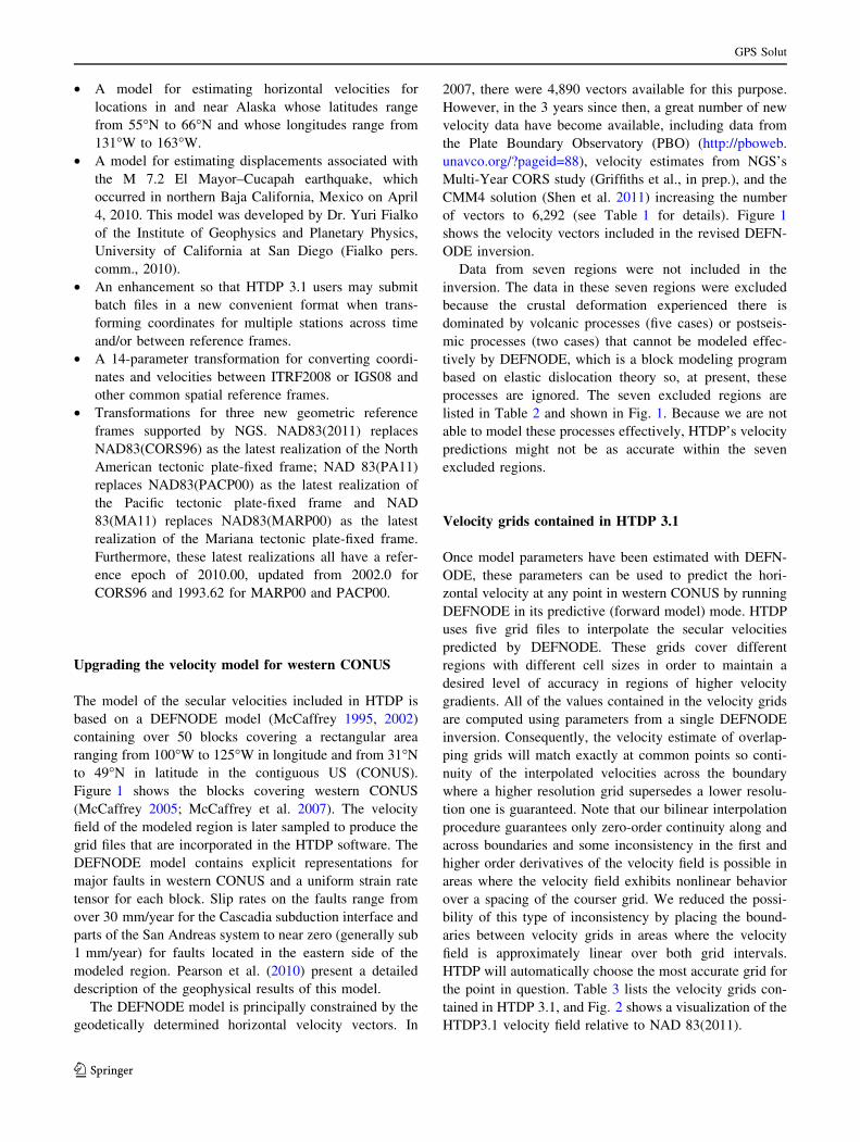
Figure 1 shows the blocks covering western CONUS

(McCaffrey 2005; McCaffrey et al. 2007). The velocity

field of the modeled region is later sampled to produce the

grid files that are incorporated in the HTDP software. The

DEFNODE model contains explicit representations for

major faults in western CONUS and a uniform strain rate

tensor for each block. Slip rates on the faults range from

over 30 mm/year for the Cascadia subduction interface and

parts of the San Andreas system to near zero (generally sub

1 mm/year) for faults located in the eastern side of the

modeled region. Pearson et al. (2010) present a detailed

description of the geophysical results of this model.

The DEFNODE model is principally constrained by the

geodetically determined horizontal velocity vectors. In

2007, there were 4,890 vectors available for this purpose.

However, in the 3 years since then, a great number of new

velocity data have become available, including data from

the Plate Boundary Observatory (PBO) (http://pboweb.

unavco.org/?pageid=88), velocity estimates from NGS’s

Multi-Year CORS study (Griffiths et al., in prep.), and the

CMM4 solution (Shen et al. 2011) increasing the number

of vectors to 6,292 (see Table 1 for details). Figure 1

shows the velocity vectors included in the revised DEFN-

ODE inversion.

Data from seven regions were not included in the

inversion. The data in these seven regions were excluded

because the crustal deformation experienced there is

dominated by volcanic processes (five cases) or postseis-

mic processes (two cases) that cannot be modeled effec-

tively by DEFNODE, which is a block modeling program

based on elastic dislocation theory so, at present, these

processes are ignored. The seven excluded regions are

listed in Table 2 and shown in Fig. 1. Because we are not

able to model these processes effectively, HTDP’s velocity

predictions might not be as accurate within the seven

excluded regions.

Velocity grids contained in HTDP 3.1

Once model parameters have been estimated with DEFN-

ODE, these parameters can be used to predict the hori-

zontal velocity at any point in western CONUS by running

DEFNODE in its predictive (forward model) mode. HTDP

uses five grid files to interpolate the secular velocities

predicted by DEFNODE. These grids cover different

regions with different cell sizes in order to maintain a

desired level of accuracy in regions of higher velocity

gradients. All of the values contained in the velocity grids

are computed using parameters from a single DEFNODE

inversion. Consequently, the velocity estimate of overlap-

ping grids will match exactly at common points so conti-

nuity of the interpolated velocities across the boundary

where a higher resolution grid supersedes a lower resolu-

tion one is guaranteed. Note that our bilinear interpolation

procedure guarantees only zero-order continuity along and

across boundaries and some inconsistency in the first and

higher order derivatives of the velocity field is possible in

areas where the velocity field exhibits nonlinear behavior

over a spacing of the courser grid. We reduced the possi-

bility of this type of inconsistency by placing the bound-

aries between velocity grids in areas where the velocity

field is approximately linear over both grid intervals.

HTDP will automatically choose the most accurate grid for

the point in question. Table 3 lists the velocity grids con-

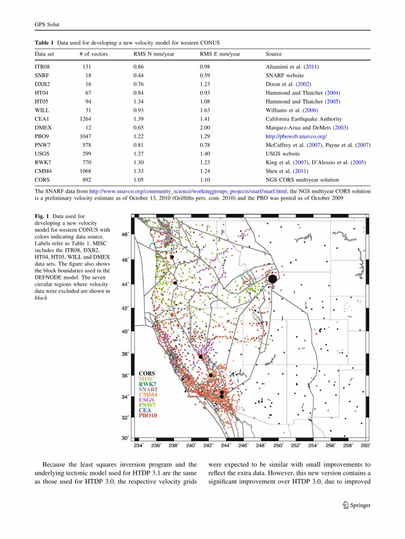
tained in HTDP 3.1, and Fig. 2 shows a visualization of the

HTDP3.1 velocity field relative to NAD 83(2011).

GPS Solut

123

Because the least squares inversion program and the

underlying tectonic model used for HTDP 3.1 are the same

as those used for HTDP 3.0, the respective velocity grids

were expected to be similar with small improvements to

reflect the extra data. However, this new version contains a

significant improvement over HTDP 3.0, due to improved

Fig. 1 Data used for

developing a new velocity

model for western CONUS with

colors indicating data source.

Labels refer to Table 1. MISC

includes the ITR08, DXB2,

HT04, HT05, WILL and DMEX

data sets. The figure also shows

the block boundaries used in the

DEFNODE model. The seven

circular regions where velocity

data were excluded are shown in

black

Table 1 Data used for developing a new velocity model for western CONUS

Data set # of vectors RMS N mm/year RMS E mm/year Source

ITR08 131 0.86 0.98 Altamimi et al. (2011)

SNRF 18 0.44 0.59 SNARF website

DXB2 16 0.76 1.23 Dixon et al. (2002)

HT04 67 0.84 0.93 Hammond and Thatcher (2004)

HT05 94 1.34 1.08 Hammond and Thatcher (2005)

WILL 31 0.93 1.63 Williams et al. (2006)

CEA1 1264 1.39 1.41 California Earthquake Authority

DMEX 12 0.65 2.00 Marquez-Azua and DeMets (2003)

PBO9 1047 1.22 1.29 http://pboweb.unavco.org/

PNW7 578 0.81 0.78 McCaffrey et al. (2007), Payne et al. (2007)

USGS 299 1.27 1.40 USGS website

RWK7 770 1.30 1.23 King et al. (2007), D’Alessio et al. (2005)

CMM4 1068 1.33 1.24 Shen et al. (2011)

CORS 892 1.05 1.10 NGS CORS multiyear solution

The SNARF data from http://www.unavco.org/community_science/workinggroups_projects/snarf/snarf.html, the NGS multiyear CORS solution

is a preliminary velocity estimate as of October 13, 2010 (Griffiths pers. com. 2010) and the PBO was posted as of October 2009

GPS Solut

123

handling of the creeping section of the San Andreas fault

where the two sides of the fault slip past each other in

opposite directions producing a spatial discontinuity in the

velocity field. This section of the fault is problematic

because HTDP uses bilinear interpolation to estimate point

velocities in each grid cell. The HTDP 3.0 velocity grid—

with a 3.75 ‘‘by 3.75’’ spacing—was too coarse to follow

the very sudden velocity change across this segment of the

San Andreas fault. To deal with this deformation, NGS

added a new velocity grid with a 0.6 ‘‘by 0.6’’ spacing in

the vicinity of the fault. Although no grid can perfectly

represent this discontinuous change in velocities, the new

finer grid follows the change better. The pixel size in this

figure represents the cell spacing in the HTDP velocity

grid, coarse in the east where the velocities change very

slowly and becoming finer in the tectonically active regions

along the west coast. This figure shows a very strong

velocity gradient across California south of Cape Mendo-

cino due to the presence of the San Andreas fault. Veloc-

ities range from over 50 mm/year in the coastal regions to

less than 10 mm/year in the eastern boundaries of the state.

Farther north in Washington and Oregon, the velocity

gradient is much more restrained because the major plate

boundary fault there is the Cascadia Subduction Zone,

which is located over 50 km off shore.

Test of the CONUS velocity grids

We used a set of 1,271 velocity vectors provided by the

California Spatial Reference Center (Yehuda Bock 2011,

pers. comm.) to validate the velocity field for western

CONUS. These velocity vectors provide an independent

Table 2 Circular regions where

velocity data were excludedName Center latitude Center longitude Radius km

deg deg

Mammoth Lakes Volcanic Region 37.8 118.9 20

Coso Volcanic Field 36 117.75 20

Yellowstone Volcanic Region 44.43 110.67 50

South Sister Volcano 44.1 121.85 20

Mount St Helens Volcano 46.2 122.18 20

Landers earthquake 34 116.5 20

Landers earthquake 34 116.5 20

Table 3 Velocity grids used in HTDP 3.1

Longitude range Latitude range Cell spacing (min) Grid dimensions Region

100�–125�W 31�–49�N 15 101 9 73 Entire region

122�–125�W 40�–49�N 3.75 49 9 145 Pacific NW

119�–125�W 36�–40�N 3.75 97 9 65 Northern CA

114�–121�W 31�–36�N 3.75 113 9 81 Southern CA

120.51�–121.4�W 35.8�–36.79�N 0.6 130 9 100 Slipping San Andreas

131�–163�W 55�–66�N 15 45 9 129 Alaska

Fig. 2 Visualization of the HTDP3.1 velocity field relative to NAD

83(2011). Predicted velocities on 1 degree grid are shown in black.

The pixel size in this figure represents the cell spacing in the HTDP

velocity grid, coarse in the east where the velocities change very

slowly and becoming finer in the tectonically active regions along the

west coast. The inset provides greater detail for the velocity field in

central California

GPS Solut

123

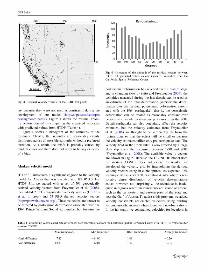
test because they were not used as constraints during the

development of our model (http://sopac.ucsd.edu/pro

cessing/coordinates/). Figure 3 shows the residual veloc-

ity vectors derived by comparing the measured velocities

with predicted values from HTDP (Table 4).

Figure 4 shows a histogram of the azimuths of the

residuals. Clearly, the azimuths are reasonably evenly

distributed across all possible azimuths without a preferred

direction. As a result, the misfit is probably caused by

random errors and there does not seem to be any evidence

of a bias.

Alaskan velocity model

HTDP 3.1 introduces a significant upgrade to the velocity

model for Alaska that was encoded into HTDP 3.0. For

HTDP 3.1, we started with a set of 591 geodetically

derived velocity vectors from Freymueller et al. (2008),

then added 23 CORS-generated velocity vectors (Griffiths

et al. in prep.) and 53 PBO derived velocity vectors

(http://pboweb.unavco.org/). These velocities are known to

be affected by postseismic deformation associated with the

1964 Prince William Sound earthquake, but because the

postseismic deformation has reached such a mature stage

and is changing slowly (Suito and Freymueller 2009), the

velocities measured during the last decade can be used as

an estimate of the total deformation (interseismic defor-

mation plus the residual postseismic deformation associ-

ated with the 1964 earthquake), that is, the postseismic

deformation can be treated as reasonably constant over

periods of a decade. Postseismic processes from the 2002

Denali earthquake can also potentially affect the velocity

estimates, but the velocity estimates from Freymueller

et al. (2008) are thought to be sufficiently far from the

rupture zone so that the effect will be small or because

the velocity estimates utilize only pre-earthquake data. The

velocity field in the Cook Inlet is also effected by a large

slow slip event that occurred between 1998 and 2001

(Freymueller et al. 2008). The available velocity vectors

are shown in Fig. 5. Because the DEFNODE model used

for western CONUS does not extend to Alaska, we

developed the velocity grid by interpolating the derived

velocity vectors using bi-cubic splines. As expected, this

technique works very well in central Alaska where a rea-

sonably dense distribution of velocity determinations

exists; however, not surprisingly, the technique is inade-

quate in regions where measurements are sparse or absent,

such as the far western and eastern parts of the State and

near the Gulf of Alaska. To address this problem, we added

velocity constraints (calculated velocities using existing

tectonic models) in areas where there were no observations.

In the far south, we constrained velocities for locations in

Fig. 3 Residual velocity vectors for the CSRC test points

Table 4 Comparing vector-coordinate differences between velocities from the California Spatial Reference Center with HTDP 3.1 velocities for

western CONUS

Max (mm/year) Min (mm/year) RMS (mm/year) Average (mm/year)

North difference 7.42 -14.00 1.49 -0.26

East difference 12.51 -12.07 1.42 -0.03

Fig. 4 Histogram of the azimuth of the residual vectors between

HTDP 3.1 predicted velocities and measured velocities from the

California Spatial Reference Center

GPS Solut

123

the central Gulf of Alaska to the Pacific plate rate. In the far

west, we used velocities from the Bering plate model

proposed by Cross and Freymueller (2007, 2008); and for

eastern Alaska and adjacent parts of northern British

Columbia and the Yukon, we used the Baranof and

Northern Cordillera block models from Elliott et al. (2010).

These block motions represent only the stable interseismic

velocities, in contrast to some of the measured velocities

discussed above that include the combined effects of in-

terseismic deformation plus the residual postseismic

deformation associated with the 1964 earthquake. How-

ever, these velocity estimates are for areas that are located

sufficiently far from the rupture zone of the 1964 earth-

quake, so postseismic effects would be small. Because both

the Cross and Freymueller model and the Elliot et al. model

were calculated in a North America-fixed frame developed

using the Euler pole for North America presented by Sella

et al. (2007), we used the same pole to rotate the predicted

velocities for all three blocks back into the ITRF2000

reference system. These point velocity estimates and the

velocity estimates from Freymueller et al. (2008) were later

transformed into the ITRF2005 reference system so that all

the velocities could be gridded in a common datum. The

resulting grid was later transformed into ITRF2008 using a

beta version of HTDP 3.1.

Alaskan velocity field

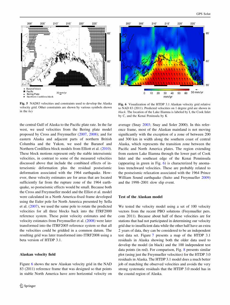
Figure 6 shows the new Alaskan velocity grid in the NAD

83 (2011) reference frame that was designed so that points

in stable North America have zero horizontal velocity on

average (Snay 2003; Snay and Soler 2000). In this refer-

ence frame, most of the Alaskan mainland is not moving

significantly with the exception of a zone of between 200

and 300 km in width along the southern coast of central

Alaska, which represents the transition zone between the

Pacific and North America plates. The region extending

from eastern Lake Iliamna through the lower part of Cook

Inlet and the southeast edge of the Kenai Penninsula

(appearing in green in Fig. 6) is characterized by anoma-

lous trenchward velocities. These are probably related to

the postseismic relaxation associated with the 1964 Prince

William Sound earthquake (Suito and Freymueller 2009)

and the 1998–2001 slow slip event.

Test of the Alaskan model

We tested the velocity model using a set of 100 velocity

vectors from the recent PBO solutions (Freymueller pers.

com 2011). Because about half of these velocities are for

stations that had not participated in determining our velocity

grid due to insufficient data while the other half have an extra

2 years of data, they can be considered to be an independent

test data set. Figure 7 presents a map of the HTDP 3.1

residuals in Alaska showing both the older data used to

develop the model (in black) and the 100 independent test

data points (in red). For comparison, Fig. 8 presents similar

plot (using just the Freymueller velocities) for the HTDP 3.0

residuals in Alaska. The HTDP 3.1 model does a much better

job of matching the observed velocities and avoids the very

strong systematic residuals that the HTDP 3.0 model has in

the coastal region of Alaska.

Fig. 5 NAD83 velocities and constraints used to develop the Alaska

velocity grid. Other constraints are shown by various symbols shown

in the key

Fig. 6 Visualization of the HTDP 3.1 Alaskan velocity grid relative

to NAD 83 (2011). Predicted velocities on 1 degree grid are shown in

black. The location of the Lake Iliamna is labeled by I, the Cook Inlet

by C, and the Kenai Peninsula by K

GPS Solut

123

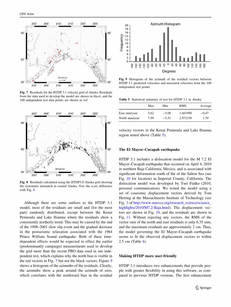
Although there are some outliers to the HTDP 3.1

model, most of the residuals are small and (for the most

part) randomly distributed, except between the Kenai

Peninsula and Lake Iliamna where the residuals show a

consistently northerly trend. This may be caused by the end

of the 1998–2001 slow slip event and the gradual decrease

in the postseismic relaxation associated with the 1964

Prince William Sound earthquake. Both of these time-

dependent effects would be expected to effect the earlier

(predominantly campaign) measurements used to develop

the grid more than the recent PBO data used in our inde-

pendent test, which explains why the north bias is visible in

the red vectors in Fig. 7 but not the black vectors. Figure 9

shows a histogram of the azimuths of the residuals. Clearly,

the azimuths show a peak around the azimuth of zero,

which correlates with the northward bias in the residual

velocity vectors in the Kenai Peninsula and Lake Iliamna

region noted above (Table 5).

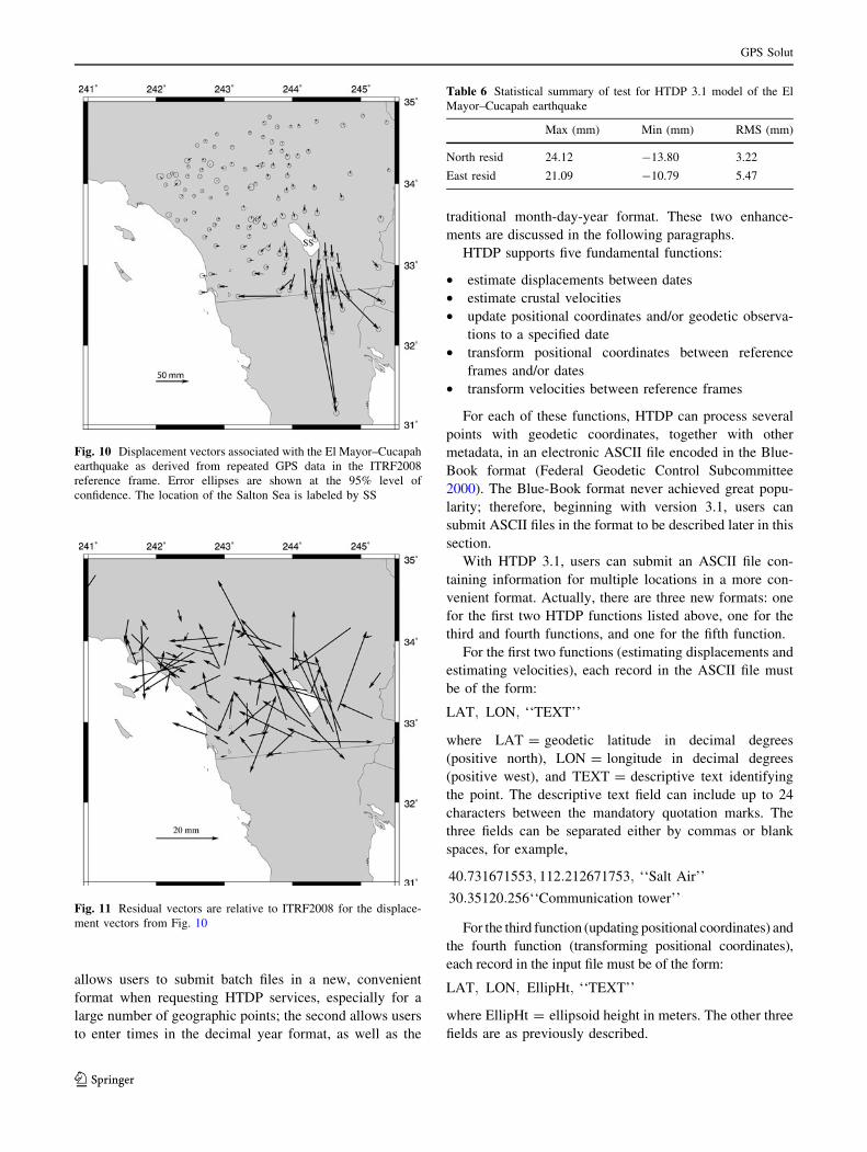
The El Mayor–Cucapah earthquake

HTDP 3.1 includes a dislocation model for the M 7.2 El

Mayor–Cucapah earthquake that occurred on April 4, 2010

in northern Baja California, Mexico, and is associated with

significant deformation south of the of the Salton Sea (see

Fig. 10 for location) in Imperial County, California. The

dislocation model was developed by Yuri Fialko (2010,

personal communication). We tested the model using a

set of coseismic displacement vectors derived by Tom

Herring at the Massachusetts Institute of Technology (see

Fig. 3 of http://www.unavco.org/research_science/science_

highlights/2010/M7.2-Baja.html). The displacement vec-

tors are shown in Fig. 10, and the residuals are shown in

Fig. 11. Without rejecting any vectors, the RMS of the

vector sum of the north and east residuals is only 6.35 mm,

and the maximum residuals are approximately 2 cm. Thus,

the model governing the El Mayor–Cucapah earthquake

seems to fit the observed displacement vectors to within

2.5 cm (Table 6).

Making HTDP more user-friendly

HTDP 3.1 introduces two enhancements that provide peo-

ple with greater flexibility in using this software, as com-

pared to previous HTDP versions. The first enhancement

Fig. 7 Residuals for the HTDP 3.1 velocity grid of Alaska. Residuals

from the data used to develop the model are shown in black, and the

100 independent test data points are shown in red

Fig. 8 Residuals calculated using the HTDP3.0 Alaska grid showing

the systematic mismatch in coastal Alaska. Note the scale difference

with Fig. 8

Fig. 9 Histogram of the azimuth of the residual vectors between

HTDP 3.1 predicted velocities and measured velocities from the 100

independent test points

Table 5 Statistical summary of test for HTDP 3.1 in Alaska

Max Min RMS Average

East mm/year 5.62 -5.08 1.661998 -0.47

North mm/year 7.99 -5.51 2.972158 1.39

GPS Solut

123

allows users to submit batch files in a new, convenient

format when requesting HTDP services, especially for a

large number of geographic points; the second allows users

to enter times in the decimal year format, as well as the

traditional month-day-year format. These two enhance-

ments are discussed in the following paragraphs.

HTDP supports five fundamental functions:

• estimate displacements between dates

• estimate crustal velocities

• update positional coordinates and/or geodetic observa-

tions to a specified date

• transform positional coordinates between reference

frames and/or dates

• transform velocities between reference frames

For each of these functions, HTDP can process several

points with geodetic coordinates, together with other

metadata, in an electronic ASCII file encoded in the Blue-

Book format (Federal Geodetic Control Subcommittee

2000). The Blue-Book format never achieved great popu-

larity; therefore, beginning with version 3.1, users can

submit ASCII files in the format to be described later in this

section.

With HTDP 3.1, users can submit an ASCII file con-

taining information for multiple locations in a more con-

venient format. Actually, there are three new formats: one

for the first two HTDP functions listed above, one for the

third and fourth functions, and one for the fifth function.

For the first two functions (estimating displacements and

estimating velocities), each record in the ASCII file must

be of the form:

LAT; LON; ‘‘TEXT’’

where LAT = geodetic latitude in decimal degrees

(positive north), LON = longitude in decimal degrees

(positive west), and TEXT = descriptive text identifying

the point. The descriptive text field can include up to 24

characters between the mandatory quotation marks. The

three fields can be separated either by commas or blank

spaces, for example,

40:731671553; 112:212671753; ‘‘Salt Air’’

30:35120:256‘‘Communication tower’’

For the third function (updating positional coordinates) and

the fourth function (transforming positional coordinates),

each record in the input file must be of the form:

LAT; LON; EllipHt; ‘‘TEXT’’

where EllipHt = ellipsoid height in meters. The other three

fields are as previously described.

Fig. 10 Displacement vectors associated with the El Mayor–Cucapah

earthquake as derived from repeated GPS data in the ITRF2008

reference frame. Error ellipses are shown at the 95% level of

confidence. The location of the Salton Sea is labeled by SS

Fig. 11 Residual vectors are relative to ITRF2008 for the displace-

ment vectors from Fig. 10

Table 6 Statistical summary of test for HTDP 3.1 model of the El

Mayor–Cucapah earthquake

Max (mm) Min (mm) RMS (mm)

North resid 24.12 -13.80 3.22

East resid 21.09 -10.79 5.47

GPS Solut

123

HTDP can provide updated or transformed 3-D geo-

centric Cartesian coordinates as well as 3-D geodetic

coordinates (geodetic latitude, longitude, and ellipsoid

height). The third function also enables users to update

geodetic observations such as interstation GPS vectors

(GPS baselines), distances, azimuths, and directions.

Unfortunately, HTDP 3.1 can only accept values for these

observations, together with appropriate metadata, in the

Blue-Book format, as is the case with previous HTDP

versions.

For the fifth function (transforming velocities between

reference frames), each record in the input file must be of

the form:

LAT; LON; Vn; Ve; Vu; ‘‘TEXT’’

where Vn = the north–south component of velocity in

mm/year (positive northward), Ve = the east–west com-

ponent of velocity in mm/year (positive eastward), and

Vu = the up-down component of velocity in mm/year

(positive upward). The other three fields are as previously

described.

As mentioned above, HTDP 3.1 now allows users to

enter dates in the decimal year format, which is the format

utilized for dates appearing in NGS geodetic control

Datasheets and Online Positioning User Service (OPUS)

reports. With previous HTDP versions, users could only

enter dates in the month-day-year format. Users need to

provide dates to HTDP when performing functions 1, 3,

and 4.

A date in the decimal year format can be of the form

yyyy.xxx where yyyy denotes the year and xxx denotes the

fraction of year. Valid examples are

2010:0 for January 1; 2010

1979:359 for May 12; 1979:

The decimal point is required, but the precision is optional.

That is, a user may enter yyyy. or yyyy.xxxxxx where any

reasonable number of ‘‘x’’ may follow the decimal point.

HTDP actually uses the decimal year representation for its

internal computations. When a user provides a date in the

month-day-year format, HTDP subtracts one from the

Julian day number and divides this difference by 365 (or

366 if a leap year) to obtain the fraction of the year. Thus,

the computed fraction corresponds to UTC midnight at the

beginning of the day.

Conclusions

HTDP 3.1 includes upgraded models of the velocity field for

both CONUS and Alaska and a model for the El Mayor–

Cucapah earthquake. In particular, the improvement for

Alaska is probably the most important change because the

previous velocity model had a significant bias of about

30 mm/year in south-central Alaska. In addition, adding the

El Mayor–Cucapah earthquake is important because it is the

largest earthquake to affect CONUS since the 1992 M 7.5

Landers earthquake. The El Mayor–Cucapah earthquake is

associated with significant deformation in the vicinities of the

Salton Sea and the cities of El Centro and Calexico in Imperial

County, California. The new velocity grids for CONUS

included in this version of HTDP utilize two additional years

of PBO data plus velocity vectors derived as part of the Multi-

Year CORS reprocessing performed by NGS. HTDP 3.1

shows a small but significant improvement in fit for western

CONUS as compared to HTDP 3.0. We also added a smaller-

spaced grid to better resolve the velocity variation occurring

near the creeping segment of California’s San Andreas fault.

HTDP 3.1 also incorporates 14-parameter transformations

between ITRF2008 and other popular reference frames. The

Appendix presents equations for transforming ITRF2008

coordinates between ITRF2008 and each of three different

plate-fixed realizations of the North American Datum of 1983

(NAD 83).

Acknowledgments Rob McCaffrey of Portland State University

developed the original DEFNODE model of western CONUS while

under contract to the National Geodetic Survey in 2007. We grate-

fully acknowledge Jeff Freymueller of the University of Alaska,

Fairbanks who hosted one of us (Chris Pearson) on two occasions and

suggested that we develop the Alaskan deformation model described

here. Thanks are also due to Dr. Yuri Fialko of University of Cali-

fornia San Diego (UCSD) for making his dislocation model of the El

Mayor—Cucapah earthquake available prior to publication. The

paper has significantly benefited from reviews by Marti Ikehara, Dave

Minkel and Dru Smith of National Geodetic Survey, Duncan Agnew

of UCSD and Thomas Meyer of the University of Connecticut.

Appendix: Transforming coordinates

between ITRF2008 and NAD 83

This appendix presents equations for transforming posi-

tional coordinates between ITRF2008 and NAD 83

(CORS96). We also present equations for transforming

positional coordinates between ITRF2008 and NAD 83

(PACP00), as well as equations for transforming positional

coordinates between ITRF2008 and NAD 83 (MARP00).

These equations were incorporated into HTDP 3.1. In the

following text, the names—NAD 83 (CORS96), NAD 83

(PACP00), and NAD 83 (MARP00)—will be truncated to

NAD 83 when referring to these three NAD 83 realizations

collectively.

Let x(t)NAD 83, y(t)NAD 83 and z(t)NAD 83 denote the NAD

83 positional coordinates for a point at time t as expressed

in a 3-D Cartesian earth-centered, earth-fixed coordinate

system. These coordinates are expressed as a function of

GPS Solut

123

time to reflect the reality of the crustal motion associated

with plate tectonics, land subsidence, volcanic activity,

postglacial rebound and so on. Similarly, let x(t)ITRF,

y(t)ITRF and z(t)ITRF denote the ITRF2008 positional

coordinates for this same point at time t. The given

ITRF2008 coordinates are related to their corresponding

NAD 83 coordinates by a similarity transformation that is

approximated by the following equations

xðtÞNAD83 ¼ TxðtÞ þ ½1þ sðtÞ� � xðtÞITRF

þ xzðtÞ � yðtÞITRF � xyðtÞ � zðtÞITRF

yðtÞNAD83 ¼ TyðtÞ � xzðtÞ � xðtÞITRF þ ½1þ sðtÞ� � yðtÞITRF

þ xxðtÞ � zðtÞITRF

zðtÞNAD83 ¼ TzðtÞ þ xyðtÞ � xðtÞITRF � xxðtÞ � yðtÞITRF

þ ½1þ sðtÞ� � zðtÞITRF ð1Þ

Here, the symbols Tx(t), Ty(t), and Tz(t) are translations

along the x-, y-, and z-axes, respectively; xx(t), xy(t), and

xz(t) are counterclockwise rotations about these same three

axes; and s(t) is the differential scale change between

ITRF2008 and NAD 83. These approximate equations

suffice because the three rotations have small magnitudes.

Note that each of the seven quantities is represented as a

function of time because space-based geodetic techniques

have enabled scientists to detect their time-related

variations with some degree of accuracy. These time-

related variations are assumed to be mostly linear, so that

the quantities may be expressed by the following equations,

Tx tð Þ ¼ Tx t0ð Þ þ _Tx � t � t0ð ÞTy tð Þ ¼ Ty t0ð Þ þ _Ty � t � t0ð ÞTz tð Þ ¼ Tz t0ð Þ þ _Tz � t � t0ð Þxx tð Þ ¼ ½ex t0ð Þ þ _ex � t � t0ð Þ� � mr

xy tð Þ ¼ ½ey t0ð Þ þ _ey � t � t0ð Þ� � mr

xz tð Þ ¼ ½ez t0ð Þ þ _ez � t � t0ð Þ� � mr

s tð Þ ¼ s t0ð Þ þ _s � t � t0ð Þ

ð2Þ

where mr = 4.84813681 � 10-9 is the conversion factor

from milliarc seconds (mas) to radians.

Here, the symbol t0 denotes a fixed, prespecified time of

reference. Hence the seven quantities Tx(t0), Ty(t0),…, s(t0)

are all constants. The seven other quantities _Tx, _Ty,…, _s,

which represents rates of change with respect to time, are

also assumed to be constants.

The transformation from ITRF2008 to NAD 83

(CORS96), denoted (ITRF2008?NAD 83 (CORS96)), is

defined in terms of the composition of five distinct trans-

formations, applied sequentially. First, positional coordi-

nates are transformed from ITRF2008 to ITRF2005, then

from ITRF2005 to ITRF2000, then from ITRF2000 to

ITRF97, then from ITRF97 to ITRF96, and finally from

ITRF96 to NAD 83 (CORS96). This composition may be

symbolically expressed via the following equation:

ITRF2008! NAD 83 CORS96ð Þð Þ ¼ ITRF2008! ITRF2005ð Þþ ITRF2005! ITRF2000ð Þ þ ITRF2000! ITRF97ð Þþ ITRF97! ITRF96ð Þ þ ITRF96! NAD 83 CORS96ð Þð Þ

ð3Þ

where (ITRF2008?ITRF2005) denotes the transformation

from ITRF2008 to ITRF2005, (ITRF2005?ITRF2000)

denotes the transformation from ITRF2005 to ITRF2000,

and so forth.

For (ITRF2008?ITRF2005), HTDP uses the parameter

values adopted by the International Earth Rotation and

Reference System Service (IERS) for t0 = 2005.00 (*1

January 2005) (Altamimi et al. 2011). We have converted

the IERS-adopted values for t0 = 2005.00 to their corre-

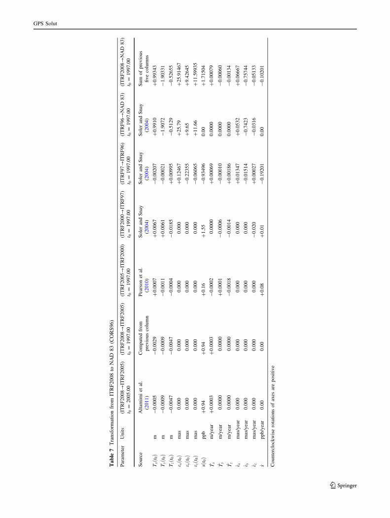
sponding values for t0 = 1997.00. Table 7 displays both

sets of values.

For (ITRF2005?ITRF2000), HTDP uses the parame-

ters adopted by the IERS for t0 = 2000.00 (Altamimi et al.

2007). The corresponding values for t0 = 1997.00 are

given by Pearson et al. (2010).

For (ITRF2000?ITRF97), (ITRF97?ITRF96), and

(ITRF96?NAD 83 (CORS96)), HTDP uses the parameter

values adopted by NGS for t0 = 1997.00 (Soler and Snay

2004). Table 7 summarizes the values adopted for all

transformations at t0 = 1997.00.

Because the values for the parameters associated with

each of the five transformations, appearing on the right side

of equation (A3), are rather small in magnitude, the values

for the parameters of (ITRF2008?NAD 83 (CORS96)) at

t0 = 1997.00 may be computed with sufficient accuracy by

adding the corresponding values for these five transfor-

mations at t0 = 1997.00. The right-most column of Table 7

displays the resulting values used by HTDP. It should be

noted that many of the values, given in Table 7, are

expressed to more significant digits than the accuracy to

which they can be resolved using current geodetic obser-

vations. Nevertheless, HTDP uses these values. The

inverse transformation (NAD 83 (CORS96)?ITRF2008)

at t0 = 1997.00 is obtained by changing the sign for each

of the 14 values appearing in the right-most column of

Table 7.

Transforming coordinates between ITRF2008 and NAD

83 (PACP00)

Snay (2003) introduced the NAD 83 (PACP00) realization

of a Pacific plate-fixed version of the NAD 83 reference

frame so that points located in the stable interior of the

Pacific tectonic plate would experience little or no

GPS Solut

123

Ta

ble

7T

ran

sfo

rmat

ion

fro

mIT

RF

20

08

toN

AD

83

(CO

RS

96

)

Par

amet

erU

nit

s(I

TR

F2

00

8?

ITR

F2

00

5)

t 0=

20

05.0

0

(IT

RF

200

8?

ITR

F2

00

5)

t 0=

19

97

.00

(IT

RF

20

05?

ITR

F2

00

0)

t 0=

19

97.0

0

(IT

RF

20

00?

ITR

F9

7)

t 0=

19

97.0

0

(IT

RF

97?

ITR

F9

6)

t 0=

19

97.0

0

(IT

RF

96?

NA

D8

3)

t 0=

19

97.0

0

(IT

RF

200

8?

NA

D8

3)

t 0=

19

97

.00

So

urc

eA

ltam

imi

etal

.

(20

11)

Com

pu

ted

fro

m

pre

vio

us

colu

mn

Pea

rso

net

al.

(20

10)

So

ler

and

Sn

ay

(20

04)

So

ler

and

Sn

ay

(20

04)

So

ler

and

Sn

ay

(20

04)

Su

mo

fp

rev

iou

s

fiv

eco

lum

ns

Tx

t 0ðÞ

m-

0.0

00

5-

0.0

02

9?

0.0

00

7?

0.0

06

7-

0.0

02

07

?0

.99

10

?0

.993

43

Ty

t 0ðÞ

m-

0.0

00

9-

0.0

00

9-

0.0

01

1?

0.0

06

1-

0.0

00

21

-1

.90

72

-1

.903

31

Tz

t 0ðÞ

m-

0.0

04

7-

0.0

04

7-

0.0

00

4-

0.0

18

5?

0.0

09

95

-0

.51

29

-0

.526

55

e xt 0ðÞ

mas

0.0

00

0.0

00

0.0

00

0.0

00

?0

.124

67

?2

5.7

9?

25

.91

46

7

e yt 0ðÞ

mas

0.0

00

0.0

00

0.0

00

0.0

00

-0

.223

55

?9

.65

?9

.426

45

e zt 0ðÞ

mas

0.0

00

0.0

00

0.0

00

0.0

00

-0

.060

65

?1

1.6

6?

11

.59

93

5

st 0ðÞ

pp

b?

0.9

4?

0.9

4?

0.1

6?

1.5

5-

0.9

34

96

0.0

0?

1.7

15

04

_ Tx

m/y

ear

?0

.00

03

?0

.000

3-

0.0

00

20

.000

0?

0.0

00

69

0.0

00

0?

0.0

00

79

_ Ty

m/y

ear

0.0

00

00

.000

0?

0.0

00

1-

0.0

00

6-

0.0

00

10

0.0

00

0-

0.0

00

60

_ Tz

m/y

ear

0.0

00

00

.000

0-

0.0

01

8-

0.0

01

4?

0.0

01

86

0.0

00

0-

0.0

01

34

_ e xm

as/y

ear

0.0

00

0.0

00

0.0

00

0.0

00

?0

.013

47

?0

.05

32

?0

.066

67

_ e ym

as/y

ear

0.0

00

0.0

00

0.0

00

0.0

00

-0

.015

14

-0

.74

23

-0

.757

44

_ e zm

as/y

ear

0.0

00

0.0

00

0.0

00

-0

.020

?0

.000

27

-0

.03

16

-0

.051

33

_sp

pb

/yea

r0

.00

0.0

0?

0.0

8?

0.0

1-

0.1

92

01

0.0

0-

0.1

02

01

Co

un

terc

lock

wis

ero

tati

on

so

fax

esar

ep

osi

tiv

e

GPS Solut

123

horizontal motion relative to this frame. NAD 83

(PACP00) is defined in terms of a transformation from

ITRF2000 of the form of Equation A2. Adopted values for

the parameters of these equations are listed in Table 8 for

t0 = 1993.62. Table 8 also presents equivalent values for

t0 = 1997.00.

The transformation from ITRF2008 to NAD 83

(PACP00), denoted (ITRF2008?NAD 83 (PACP00)), is

defined in terms of the composition of three distinct

transformations, applied sequentially. First, positional

coordinates are transformed from ITRF2008 to ITRF2005,

then from ITRF2005 to ITRF2000, and then from

ITRF2000 to NAD 83 (PACP00). This composition may be

symbolically expressed via the equation

ITRF2008! NAD 83 PACP00ð Þð Þ ¼ ITRF2008! ITRF2005ð Þþ ITRF2005! ITRF2000ð Þ þ ITRF2000! NAD 83 PACP00ð Þð Þ

ð4Þ

Table 9 displays values for the various parameters at

t0 = 1997.00, where values for the transformation from

ITRF2005 to ITRF2000 for t0 = 1997.00 were computed

by Pearson et al. (2010) from those published by Altamimi

Table 8 Transformation from

ITRF2000 to NAD 83

(PACP00)

Counterclockwise rotations of

axes are positive

Parameter Units (ITRF2000?NAD83(PACP00))

t0 = 1993.62

(ITRF2000?NAD83(PACP00))

t0 = 1997.00

Source Snay (2003) Computed from previous column

Tx t0ð Þ m 0.9102 0.9102

Ty t0ð Þ m -2.0141 -2.0141

Tz t0ð Þ m -0.5602 -0.5602

ex t0ð Þ mas 29.039 27.741

ey t0ð Þ mas 10.065 13.469

ez t0ð Þ mas 10.101 2.712

s t0ð Þ ppb 0 0

_Tx m/year 0 0

_Ty m/year 0 0

_Tz m/year 0 0

_ex mas/year -0.384 -0.384

_ey mas/year 1.007 1.007

_ez mas/year -2.186 -2.186

_s ppb/year 0 0

Table 9 Transformation from ITRF2008 to NAD 83 (PACP00)

Parameter Units (ITRF2008?ITRF2005)t0 = 1997.00

(ITRF2005?ITRF2000)t0 = 1997.00

(ITRF2000?NAD83(PACP00))t0 = 1997.00

(ITRF2008?NAD83(PACP00))t0 = 1997.00

Source Table 7 Pearson et al. (2010) Table 8 Sum of previous three columns

Tx t0ð Þ m -0.0029 0.0007 0.9102 0.908

Ty t0ð Þ m -0.0009 -0.0011 -2.0141 -2.0161

Tz t0ð Þ m -0.0047 -0.0004 -0.5602 -0.5653

ex t0ð Þ mas 0 0 27.741 27.741

ey t0ð Þ mas 0 0 13.469 13.469

ez t0ð Þ mas 0 0 2.712 2.712

s t0ð Þ ppb 0.94 0.16 0 1.1

_Tx m/year 0.0003 -0.0002 0 0.0001

_Ty m/year 0 0.0001 0 0.0001

_Tz m/year 0 -0.0018 0 -0.0018

_ex mas/year 0 0 -0.384 -0.384

_ey mas/year 0 0 1.007 1.007

_ez mas/year 0 0 -2.186 -2.186

_s ppb/year 0 0.08 0 0.08

Counterclockwise rotations of axes are positive

GPS Solut

123

et al. (2007) for t0 = 2000.00. The right-most column in

this table is obtained by adding the previous three columns

across each row.

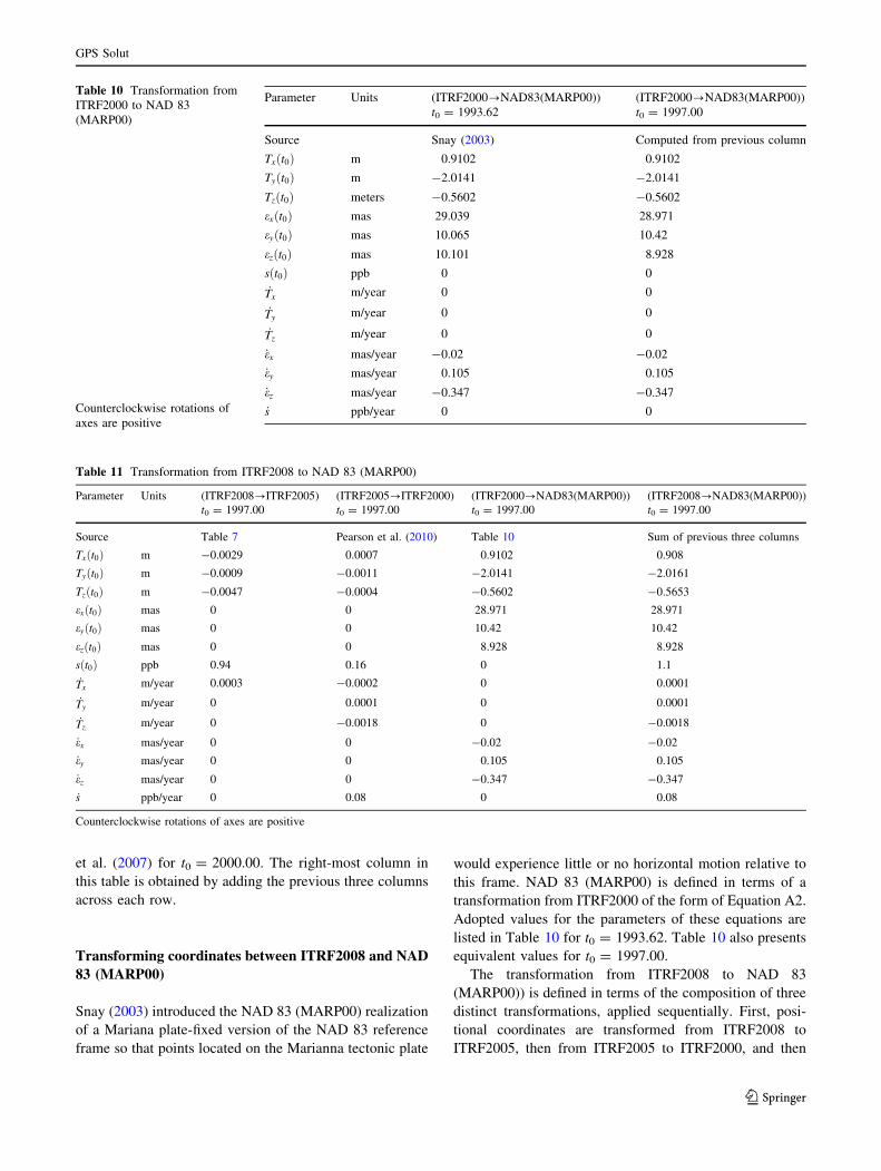
Transforming coordinates between ITRF2008 and NAD

83 (MARP00)

Snay (2003) introduced the NAD 83 (MARP00) realization

of a Mariana plate-fixed version of the NAD 83 reference

frame so that points located on the Marianna tectonic plate

would experience little or no horizontal motion relative to

this frame. NAD 83 (MARP00) is defined in terms of a

transformation from ITRF2000 of the form of Equation A2.

Adopted values for the parameters of these equations are

listed in Table 10 for t0 = 1993.62. Table 10 also presents

equivalent values for t0 = 1997.00.

The transformation from ITRF2008 to NAD 83

(MARP00)) is defined in terms of the composition of three

distinct transformations, applied sequentially. First, posi-

tional coordinates are transformed from ITRF2008 to

ITRF2005, then from ITRF2005 to ITRF2000, and then

Table 10 Transformation from

ITRF2000 to NAD 83

(MARP00)

Counterclockwise rotations of

axes are positive

Parameter Units (ITRF2000?NAD83(MARP00))

t0 = 1993.62

(ITRF2000?NAD83(MARP00))

t0 = 1997.00

Source Snay (2003) Computed from previous column

Tx t0ð Þ m 0.9102 0.9102

Ty t0ð Þ m -2.0141 -2.0141

Tz t0ð Þ meters -0.5602 -0.5602

ex t0ð Þ mas 29.039 28.971

ey t0ð Þ mas 10.065 10.42

ez t0ð Þ mas 10.101 8.928

s t0ð Þ ppb 0 0

_Tx m/year 0 0

_Ty m/year 0 0

_Tz m/year 0 0

_ex mas/year -0.02 -0.02

_ey mas/year 0.105 0.105

_ez mas/year -0.347 -0.347

_s ppb/year 0 0

Table 11 Transformation from ITRF2008 to NAD 83 (MARP00)

Parameter Units (ITRF2008?ITRF2005)

t0 = 1997.00

(ITRF2005?ITRF2000)

t0 = 1997.00

(ITRF2000?NAD83(MARP00))

t0 = 1997.00

(ITRF2008?NAD83(MARP00))

t0 = 1997.00

Source Table 7 Pearson et al. (2010) Table 10 Sum of previous three columns

Tx t0ð Þ m -0.0029 0.0007 0.9102 0.908

Ty t0ð Þ m -0.0009 -0.0011 -2.0141 -2.0161

Tz t0ð Þ m -0.0047 -0.0004 -0.5602 -0.5653

ex t0ð Þ mas 0 0 28.971 28.971

ey t0ð Þ mas 0 0 10.42 10.42

ez t0ð Þ mas 0 0 8.928 8.928

s t0ð Þ ppb 0.94 0.16 0 1.1

_Tx m/year 0.0003 -0.0002 0 0.0001

_Ty m/year 0 0.0001 0 0.0001

_Tz m/year 0 -0.0018 0 -0.0018

_ex mas/year 0 0 -0.02 -0.02

_ey mas/year 0 0 0.105 0.105

_ez mas/year 0 0 -0.347 -0.347

_s ppb/year 0 0.08 0 0.08

Counterclockwise rotations of axes are positive

GPS Solut

123

from ITRF2000 to NAD 83 (MARP00). This composition

may be symbolically expressed via the equation

ITRF2008! NAD 83 MARP00ð Þð Þ ¼ ITRF2008! ITRF2005ð Þþ ITRF2005! ITRF2000ð Þ þ ITRF2000! NAD 83 MARP00ð Þð Þ

ð5Þ

Table 11 displays values for the various parameters at

t0 = 1997.00. The right-most column in this table is obtained

by adding the previous three columns across each row.

Related transformations

The International GNSS Service(IGS) recently adopted a

reference frame called IGS08 that is based on ITRF2008.

IGS08 coordinates for some reference stations differ from

their corresponding ITRF2008 coordinates because the

IGS08 coordinates were computed using more current

calibrations of GPS antennas than were used in computing

ITRF2008 coordinates. Nevertheless, IGS considers the

14-parameter transformation between ITRF2008 and

IGS08 to be the identity function, that is, each of the 14

transformation parameters is zero in value. As a result, the

value of the 14 parameters in the transformation between

IGS08 and a given NAD 83 realization is the same as the

values of the 14 parameters in the corresponding trans-

formation between ITRF2008 and this NAD 83 realization.

Also, NGS recently adopted three new reference frames

called NAD 83 (2011), NAD 83 (PA11), and NAD 83

(MA11). To create these reference frames, NGS repro-

cessed its collection of GPS data from the CORS network

to compute IGS08 coordinates for reference stations in this

network. The corresponding NAD 83 (2011) coordinates

were then obtained by applying the (ITRF2008 ? NAD 83

(CORS96)) transformation given in this paper, which as

mentioned above is the same as the (IGS08 ? NAD 83

(CORS96)) transformation. As a result, the 14-parameter

transformation between NAD 83 (CORS96) and NAD 83

(2011) is the identity function. In most cases, NAD 83

(CORS96) coordinates for a given reference station will

differ from the corresponding NAD 83 (2011) coordinates

for this same reference frame because the NAD 83 (2011)

coordinates were computed using more GPS data, more

recent models for systematic errors (like ocean loading),

and improved mathematical algorithms than were involved

in the NAD 83 (CORS96) computations many of

which were performed in 2002. Thus, the fact that the

14-parameter transformation between two reference frames

is the identity function does not mean that corresponding

coordinates in the two frames agree exactly in value. It

only means that these corresponding coordinates agree on

average when considering all the reference stations in the

network, which have coordinates in both reference frames.

In the same manner, the transformation between

ITRF2008 (or IGS08) and NAD 83 (PA11) is the same as

the transformation between ITRF2008 and NAD 83

(PACP00), and the transformation between ITRF2008 and

NAD 83 (MA11) is the same as the transformation between

ITRF2008 and NAD 83 (MARP00). Thus, the transfor-

mation between NAD 83 (PA11) and NAD 83 (PACP00) is

the identity function, and the transformation between NAD

83 (MA11) and NAD 83 (MARP00) is also the identity

function.

References

Altamimi Z, Collilieux X, Legrand J, Garayt B, Boucher C (2007)

ITRF2005: a new release of the International Terrestrial

Reference Frame based on time series of station positions and

Earth orientation parameters. J Geophys Res. doi:10.1029/

2007JB004949

Altamimi Z, Collilieux X, Metivier L (2011) ITRF2008: an improved

solution of the international terrestrial reference frame. J Geod.

doi:10.1007/s00190-011-0444-4

Cross R, Freymueller JT (2007) Plate coupling variation and block

translation in the Andreanof segment of the Aleutian arc

determined by subduction zone modeling using GPS data.

Geophys Res Lett. doi:10.1029/2006GL029073R

Cross R, Freymueller JT (2008) Evidence for and implications of a

Bering plate based on geodetic measurements from the Aleutians

and western Alaska. J Geophys Res. doi:10.1029/2007JB005136

D’Alessio MA, Johanson IA, Burn, Schmidt DA, Murray MH (2005)

Slicing up the San Francisco Bay area: block kinematics and

fault slip rates from GPS-derived surface velocities. J Geophys

Res. doi:10.1029/2004JB003496

Dixon T, Decaix J, Farina F, Furlong K, Malservisi R, Bennett R,

Suarez-Vidal F, Fletcher J, Lee J (2002) Seismic cycle and

rheological effects on estimation of present-day slip rates for the

Agua Blanca and San Miguel-Vallecitos faults, northern Baja

California, Mexico. J Geophys Res. doi:10.1029/2000JB000099

Elliott JL, Larsen CF, Freymueller JT, Motyka RJ (2010) Tectonic

block motion and glacial isostatic adjustment in southeast Alaska

and adjacent Canada constrained by GPS measurements. J Geo-

phys Res. doi:10.1029/2009JB007139

Federal Geodetic Control Subcommittee (2000) Input formats and

specifications of the National Geodetic Survey Data Base the

NGS ‘‘Bluebook’’ http://www.ngs.noaa.gov/FGCS/BlueBook/.

Accessed 26 July 2011

Freymueller JT, Cohen SC, Cross R, Elliott J, Fletcher H, Larsen C,

Hreinsdottir S, Zweck C (2008) Active deformation processes in

Alaska, based on 15 years of GPS measurements. In: Freymu-

eller JT et al (eds) Active tectonics and seismic potential of

Alaska. AGU, Washington, DC, pp 1–42

Hammond WC, Thatcher W (2004) Contemporary tectonic deforma-

tion of the basin and range province, western United States:

10 years of observation with the Global Positioning System.

J Geophys Res. doi:10.1029/2003JB002746

Hammond WC, Thatcher W (2005) Northwest basin and range

tectonic deformation observed with the Global Positioning

System. J Geophys Res. doi:10.1029/2005JB003678

King NE, Argus D, Langbein J, Agnew DC, Bawden G, Dollar RS,

Liu Z, Galloway D, Reichard E, Yong A, Webb FH, Bock Y,

Stark K, Barseghian D (2007) Space geodetic observation of

expansion of the San Gabriel Valley, California, aquifer system,

GPS Solut

123

during heavy rainfall in winter 2004–2005. J Geophys Res. doi:

10.1029/2006JB0044

Marquez-Azua B, DeMets C (2003) Crustal velocity field of Mexico

from continuous GPS measurements, 1993 to June 2001:

implications for neotectonics of Mexico. J Geophys Res. doi:

10.1029/2002JB002241

McCaffrey R (1995) ‘‘DEFNODE users’ guide’’ Rensselaer Poly-

technic Institute, Troy, New York. http://www.rpi.edu/*mccafr/

defnode/. Accessed 8 Mar 2007

McCaffrey R (2002) Crustal block rotations and plate coupling. In:

Stein S, Freymueller J (eds), Plate boundary zones. AGU

Geodynamics Series 30, pp 101–122

McCaffrey R (2005) Block kinematics of the Pacific/North America

plate boundary in the southwestern United States from inversion

of GPS, seismological, and geologic data. J Geophys Res. doi:

10.1029/2004JB003307

McCaffrey R, Qamar AI, King RW, Wells R, Ning Z, Williams CA,

Stevens CW, Vollick JJ, Zwick PC (2007) Plate locking, block

rotation and crustal deformation in the Pacific Northwest.

Geophy J Int. doi:10.1111/j.1365-264X.2007.03371.x

Payne SJ, McCaffrey R, King RW (2007) Contemporary deformation

within the Snake River Plain and northern basin and range

province, USA. EOS Trans Am Geophys Union 88(23):T22A-05

Pearson C, McCaffrey R, Elliott JL, Snay R (2010) HTDP 3.0:

software for coping with coordinate changes associated with

crustal motion. J Surv Eng 136:80–90. doi:10.1061/(ASCE)SU.

1943-5428.0000013

Sella GF, Stein S, Dixon TH, Craymer M, James TS, Mazzotti S,

Dokka RK (2007) Observation of glacial isostatic adjustment in

‘‘stable’’ North America with GPS. Geophys Res Lett. doi:

10.1029/2006GL027081

Shen ZK, King RW, Agnew DC, Wang M, Herring TA, Dong S, Fang

P (2011) A unified analysis of crustal motion in southern

California, 1970–2004: the SCEC crustal motion map. J Geophys

Res 116 (in press)

Snay RA (2003) Introducing two spatial reference frames for regions

of the Pacific Ocean. Surv Land Inf Sci 63:5–12

Soler T, Snay RA (2004) Transforming positions and velocities

between the International Terrestrial Reference Frame of 2000

and North American Datum of 1983. J Surv Eng 130:49–55. doi:

10.1061/(ASCE)0733-9453(2004)130:2(49)

Suito H, Freymueller JT (2009) A viscoelastic and afterslip postse-

ismic deformation model for the 1964 Alaska earthquake.

J Geophys Res. doi:10.1029/2008JB005954

Williams TB, Kelsey HM, Freymueller JT (2006) GPS-derived strain

in northwestern California: termination of the San Andreas fault

system and convergence of the Sierra Nevada-Great Valley

block contribution to southern Cascadia forearc contraction.

Tectonophysics 413:171–184

Author Biographies

Chris Pearson works for the National Geodetic Survey where he is

the geodetic advisor for Illinois. He is also responsible for maintain-

ing the model of crustal deformation that NGS uses to correct

coordinates and survey data for tectonic motion in the western US.

Richard Snay served as a scientist with the U.S. National Geodetic

Survey (NGS) from 1974 to 2010. Dr. Snay managed the U.S.

Continuously Operating Reference Station (CORS) program from

1998 to 2007, and he supervised NGS’ Spatial Reference System

Division from 2003 to 2010.

GPS Solut

123