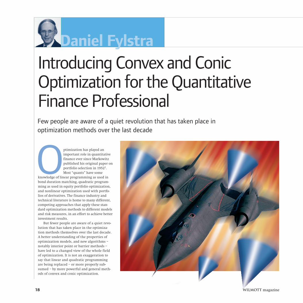
Introducing Convex and ConicOptimization for the QuantitativeFinance ProfessionalFew people are aware of a quiet revolution that has taken place in optimization methods over the last decade

Optimization has played animportant role in quantitativefinance ever since Markowitzpublished his original paper onportfolio selection in 19521.Most “quants” have some

knowledge of linear programming as used inbond duration matching, quadratic program-ming as used in equity portfolio optimization,and nonlinear optimization used with portfo-lios of derivatives. The finance industry andtechnical literature is home to many different,competing approaches that apply these stan-dard optimization methods to different modelsand risk measures, in an effort to achieve betterinvestment results.

But fewer people are aware of a quiet revo-lution that has taken place in the optimiza-tion methods themselves over the last decade.A better understanding of the properties ofoptimization models, and new algorithms –notably interior point or barrier methods –have led to a changed view of the whole fieldof optimization. It is not an exaggeration tosay that linear and quadratic programmingare being replaced – or more properly sub-sumed – by more powerful and general meth-ods of convex and conic optimization.

Daniel Fylstra

18 Wilmott magazine

Wilmott magazine 19

What this means for quantitative finance is arelaxing of restrictions on optimization models– for example, using quadratic constraints aseasily as a quadratic objective – and new ways todeal with important problems such as “unnatu-ral” portfolios from optimization that are due to“noise” in the return and covariance or factorparameters of a portfolio model. This article will introduce the ideas of convex and conicoptimization, and their applications in quantitative finance.

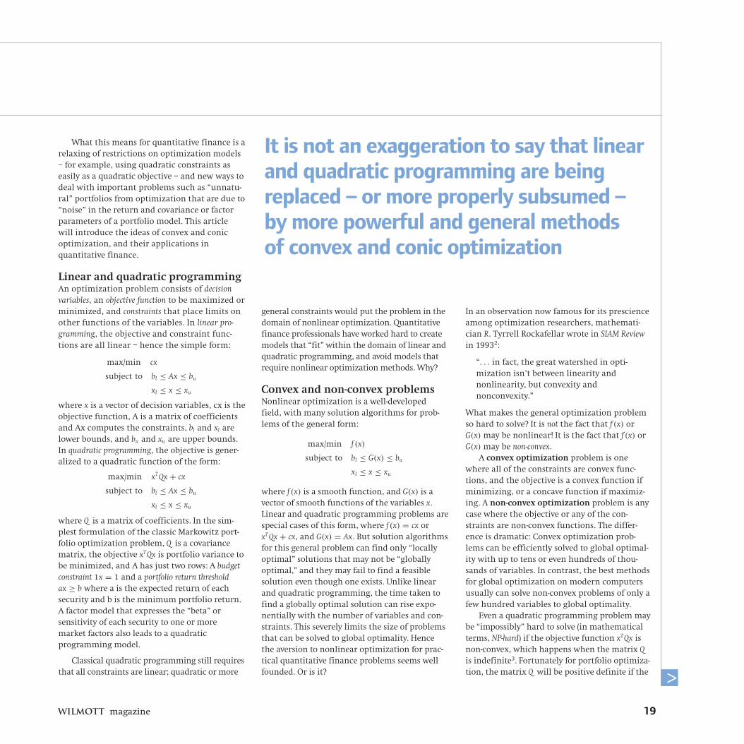
Linear and quadratic programmingAn optimization problem consists of decisionvariables, an objective function to be maximized orminimized, and constraints that place limits onother functions of the variables. In linear pro-gramming, the objective and constraint func-tions are all linear – hence the simple form:

max/min cx

subject to bl ≤ Ax ≤ bu

xl ≤ x ≤ xu

where x is a vector of decision variables, cx is theobjective function, A is a matrix of coefficientsand Ax computes the constraints, bl and xl arelower bounds, and bu and xu are upper bounds.In quadratic programming, the objective is gener-alized to a quadratic function of the form:

max/min xT Qx + cx

subject to bl ≤ Ax ≤ bu

xl ≤ x ≤ xu

where Q is a matrix of coefficients. In the sim-plest formulation of the classic Markowitz port-folio optimization problem, Q is a covariancematrix, the objective xT Qx is portfolio variance tobe minimized, and A has just two rows: A budgetconstraint 1x = 1 and a portfolio return thresholdax ≥ b where a is the expected return of eachsecurity and b is the minimum portfolio return.A factor model that expresses the “beta” or sensitivity of each security to one or more market factors also leads to a quadratic programming model.

Classical quadratic programming still requiresthat all constraints are linear; quadratic or more

general constraints would put the problem in thedomain of nonlinear optimization. Quantitativefinance professionals have worked hard to createmodels that “fit” within the domain of linear andquadratic programming, and avoid models thatrequire nonlinear optimization methods. Why?

Convex and non-convex problemsNonlinear optimization is a well-developedfield, with many solution algorithms for prob-lems of the general form:

max/min f (x)

subject to bl ≤ G(x) ≤ bu

xl ≤ x ≤ xu

where f (x) is a smooth function, and G(x) is avector of smooth functions of the variables x.Linear and quadratic programming problems arespecial cases of this form, where f (x) = cx orxT Qx + cx, and G(x) = Ax. But solution algorithmsfor this general problem can find only “locallyoptimal” solutions that may not be “globallyoptimal,” and they may fail to find a feasiblesolution even though one exists. Unlike linearand quadratic programming, the time taken tofind a globally optimal solution can rise expo-nentially with the number of variables and con-straints. This severely limits the size of problemsthat can be solved to global optimality. Hencethe aversion to nonlinear optimization for prac-tical quantitative finance problems seems wellfounded. Or is it? ^

In an observation now famous for its prescienceamong optimization researchers, mathemati-cian R. Tyrrell Rockafellar wrote in SIAM Reviewin 19932:

“. . . in fact, the great watershed in opti-mization isn’t between linearity and nonlinearity, but convexity and nonconvexity.”

What makes the general optimization problemso hard to solve? It is not the fact that f (x) orG(x) may be nonlinear! It is the fact that f (x) orG(x) may be non-convex.

A convex optimization problem is onewhere all of the constraints are convex func-tions, and the objective is a convex function ifminimizing, or a concave function if maximiz-ing. A non-convex optimization problem is anycase where the objective or any of the con-straints are non-convex functions. The differ-ence is dramatic: Convex optimization prob-lems can be efficiently solved to global optimal-ity with up to tens or even hundreds of thou-sands of variables. In contrast, the best methodsfor global optimization on modern computersusually can solve non-convex problems of only afew hundred variables to global optimality.

Even a quadratic programming problem maybe “impossibly” hard to solve (in mathematicalterms, NP-hard) if the objective function xT Qx isnon-convex, which happens when the matrix Qis indefinite3. Fortunately for portfolio optimiza-tion, the matrix Q will be positive definite if the

It is not an exaggeration to say that linearand quadratic programming are beingreplaced – or more properly subsumed – by more powerful and general methods of convex and conic optimization

models “fit” within the domain of linear andquadratic programming. For example, in Robert

Fernholz’s well-regarded work apply-ing “stochastic portfolio theory”

to equity portfolio manage-ment6, the linear portfolio

return threshold constraint isreplaced by a portfolio growth

threshold constraint thatincludes a quadratic term.

Fernholz remarks that “this con-straint is nonlinear, and conventional

quadratic programs cannot be used in thiscase.” He goes on to show that, for enhancedindex (“tracking”) portfolios, the quadratic termin the growth constraint is small in magnitude,and therefore can be neglected – yielding a lin-ear constraint and a conventional QP problem.But with modern interior point methods, thissimplification is no longer necessary – the origi-nal problem including the quadratic constraintcan be solved just as reliably, and in about thesame time, as the simplified QP problem.

Conic optimizationNesterov and Nemirovskii’s seminal work alsoopened up a natural generalization of linearprogramming, called conic programming, thatshares the favorable characteristics of LP butencompasses a wider range of problems. Andconic quadratic programming – now known assecond order cone programming – shares thefavorable characteristics of QP but encompassesa wider range problems relevant for portfoliooptimization.

20 Wilmott magazine

covariance terms are computed from historicaldata where the number of observations exceedsthe number of securities.

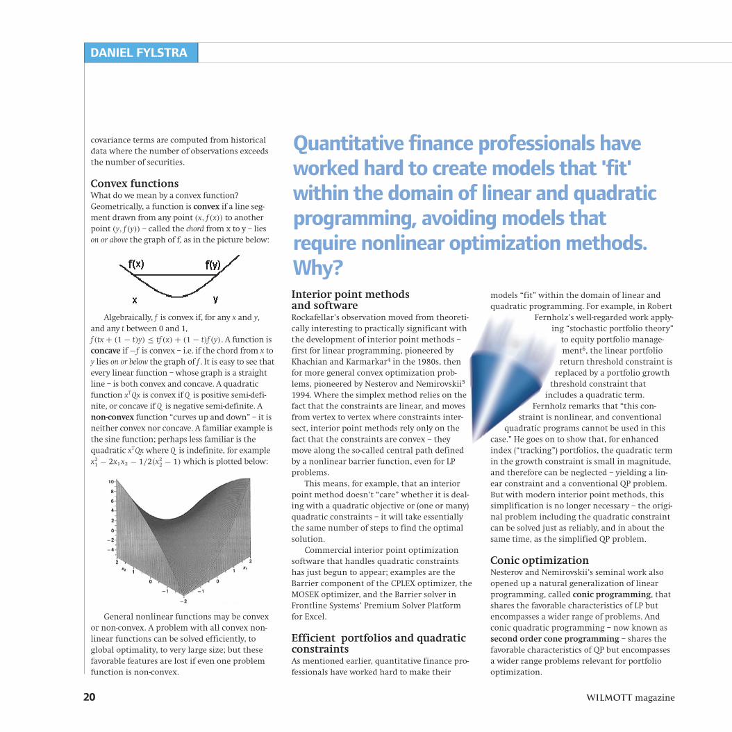
Convex functionsWhat do we mean by a convex function?Geometrically, a function is convex if a line seg-ment drawn from any point (x, f (x)) to anotherpoint (y, f (y)) – called the chord from x to y – lieson or above the graph of f, as in the picture below:

Algebraically, f is convex if, for any x and y,and any t between 0 and 1,f (tx + (1 − t)y) ≤ tf (x) + (1 − t)f (y). A function isconcave if −f is convex – i.e. if the chord from x toy lies on or below the graph of f . It is easy to see thatevery linear function – whose graph is a straightline – is both convex and concave. A quadraticfunction xT Qx is convex if Q is positive semi-defi-nite, or concave if Q is negative semi-definite. Anon-convex function “curves up and down” – it isneither convex nor concave. A familiar example isthe sine function; perhaps less familiar is thequadratic xT Qx where Q is indefinite, for examplex2

1 − 2x1x2 − 1/2(x22 − 1) which is plotted below:

General nonlinear functions may be convexor non-convex. A problem with all convex non-linear functions can be solved efficiently, toglobal optimality, to very large size; but thesefavorable features are lost if even one problemfunction is non-convex.

Interior point methods and softwareRockafellar’s observation moved from theoreti-cally interesting to practically significant withthe development of interior point methods –first for linear programming, pioneered byKhachian and Karmarkar4 in the 1980s, thenfor more general convex optimization prob-lems, pioneered by Nesterov and Nemirovskii5

1994. Where the simplex method relies on thefact that the constraints are linear, and movesfrom vertex to vertex where constraints inter-sect, interior point methods rely only on thefact that the constraints are convex – theymove along the so-called central path definedby a nonlinear barrier function, even for LPproblems.

This means, for example, that an interiorpoint method doesn’t “care” whether it is deal-ing with a quadratic objective or (one or many)quadratic constraints – it will take essentiallythe same number of steps to find the optimalsolution.

Commercial interior point optimizationsoftware that handles quadratic constraintshas just begun to appear; examples are theBarrier component of the CPLEX optimizer, theMOSEK optimizer, and the Barrier solver inFrontline Systems’ Premium Solver Platformfor Excel.

Efficient portfolios and quadraticconstraintsAs mentioned earlier, quantitative finance pro-fessionals have worked hard to make their

DANIEL FYLSTRA

Quantitative finance professionals haveworked hard to create models that 'fit'within the domain of linear and quadraticprogramming, avoiding models thatrequire nonlinear optimization methods.Why?

A conic optimization problem can be writtenas an LP – with a linear objective and linear con-straints – plus one or more cone constraints. Acone constraint specifies that the vector formedby a set of decision variables is constrained to lie within a closed convex pointed cone. Thesimplest example of such a cone is the non-nega-tive orthant, the region where all variables arenon-negative – the normal situation in an LP. But conic optimization allows for more generalcones, that can express all the elements of a port-folio optimization problem, and much more.

A simple type of closed convex pointed conethat captures many optimization problems ofinterest is the second order cone, also calledthe Lorentz cone or “ice cream cone.”Geometrically it looks like the picture below, in three dimensions:

A second order cone (SOC) constraint ofdimension n specifies that the vector formed bya set of n decision variables must belong to thiscone. Algebraically, the L2-norm of n − 1 vari-ables must be less than or equal to the mag-nitude of the nth variable. Any convexquadratic constraint can be reformulatedas an SOC constraint, though thisrequires several steps of linear algebra.A quadratic objective xT Qx can be han-dled by introducing a new variable t,making the objective “minimize t”,adding the constraint xT Qx ≤ t, and con-verting this constraint to SOC form.

A problem with a linear objective andlinear plus SOC constraints is called a sec-ond order cone programming (SOCP)problem. Such a problem can be efficient-ly solved via specialized interior point methods,in about the same time as a QP problem of thesame size. Enhancement of the simplex methodto solve SOCP problems is an area of active research, but there are not yet

commercial quality implementations of the proposed methods.

SOCP problems and portfolio optimization

One of the major problems with classicalMarkowitz portfolio optimization is

the presence of “noise” or sam-pling errors in the input dataused to estimate the terms of

the covariance matrix, or the fac-tor loadings computed for a factor

model. Michaud drew attention tothis issue in a 1998 book7, referring

to portfolio optimization as “an errorprone procedure that often results in error-

maximized and investment-irrelevant portfo-lios.” This occurs because optimization, by itsnature, maximally exploits the diversificationpotential of the data, including the estimationerrors. Resampling of the efficient frontier, pro-posed by Michaud, and various scenario-basedapproaches have been developed to cope withthis problem, but these methods do not explic-itly model parameter uncertainty or provide

DANIEL FYLSTRA

Wilmott magazine 21

^

An interior pointmethod doesn't'care' whether it isdealing with a quad-ratic objective or(one of many) quad-ratic constraints – itwill take essentiallythe same number ofsteps to find theoptimal solution

W

22 Wilmott magazine

any performance guarantees on the computedportfolio.

Goldfarb and Iyengar8 have shown howconic optimization can be applied to the sam-pling error problem in portfolio optimization.They begin with a factor model, but they treatthe mean return estimates and the factor load-ings for each security as “noisy,” belonging toparameterized uncertainty sets. They show howthe parameters of the uncertainty sets can beobtained through the normal process of linearregression used to estimate historical returnsand factor sensitivities, and how to obtain confi-dence intervals for the error in these estimatedparameters. Then they solve variations of theportfolio optimization problem (minimizingvariance, maximizing Sharpe ratio, minimizingVaR, etc.) by reformulating the constraints thatinclude the uncertain parameters as secondorder cone (SOC) constraints, with a user-speci-fied confidence threshold. The result is a portfo-lio that does offer probabilistic guarantees onrisk-return performance, and that requiresabout the same amount of computing time asconventional portfolio optimization.

Software for convex and conic problemsConic optimization, including second order coneprogramming and a related methodology calledsemidefinite programming (SDP), has been a veryactive area for optimization researchers in recentyears. Some codes developed by academics, forexample Boyd and Vandenberghe’s SOCP codeand Sturm’s SeDuMi code, can be found on theWorld Wide Web.

For quantitative finance professionals who arecomfortable working in Excel, the simplest way toexplore conic optimization is to download a freetrial version of Frontline Systems’ Premium SolverPlatform V6.0 from www.solver.com. This softwareis upward compatible from the standard ExcelSolver (that Frontline originally developed forMicrosoft) and now includes a built-in SOCPBarrier Solver. It automatically handles the linearalgebra needed to transform quadratic constraintsand objectives into SOC constraints, sparing theuser this effort. Cone constraints can be entered bysimply selecting “soc” from a drop-down list.

Hence, one can concentrate on the problem ofinterest rather than details of the software.

As noted earlier, the limitationsof nonlinear optimization – heavi-ly used in portfolios of deriva-tives – is not due to nonlineari-ty, but rather is due to non-convexity. The problem inpractice has been thatit’s very difficult formodelers to determinewhether their func-tions are convexor non-convex.It takes con-siderablemathematical expertise and time to prove con-vexity, and software to assist in this task has notbeen available. But a first-generation facility9 toautomatically determine whether a nonlinearmodel is convex or non-convex, by simply click-ing a button, is included in the Premium SolverPlatform V6.0. This makes it possible to exploreconvex optimization using any of the variety ofnonlinear optimizers available for this platform.

ConclusionsThere is growing excitement in the optimizationresearch community about the new develop-ments in convex and conic optimization – butthis is just beginning to “spill over” into thequantitative finance community, where manyusers of optimization are found. Linear and quad-ratic programming – now over fifty years old – arebeing transformed into methods more powerfuland general than ever before. Quantitative financeapplications of the new technology of convex andconic optimization are sure to grow in impor-tance over the next few years.

DANIEL FYLSTRA

1. H. Markowitz. Portfolio Selection. Journal of Finance 71: 77–91, 1952.2. T. Rockafellar. Lagrange multipliers and optimality.SIAM Review 35:183–238, 1993.3. R. Horst, P. Pardalos, N. Thoai. Introduction to GlobalOptimization. Kluwer, 1995.4. N. Karmarkar. A new polynomial-time algorithm for lin-ear programming. Combinatorica 4: 373–395, 1984.5. Y. Nesterov and A. Nemirovskii. Interior-PointPolynomial Algorithms in Convex Programming. SIAM,1994.6. R. Fernholz. The Application of Stochastic PortfolioTheory to Equity Management. INTECH research report,2003.7. R. Michaud. Efficient Asset Management. HarvardBusiness School Press, 1998.8. D. Goldfarb and G. Iyengar. Robust portfolio selectionproblems. CORC Technical Report TR-2002–03, ColumbiaUniversity.9. I. Nenov, D. Fylstra, L. Kolev. Convexity Determinationin the Microsoft Excel Solver Using AutomaticDifferentiation Techniques. Submitted for publication.

REFERENCES

The limitations of nonlinear optimization– heavily used in portfolios of derivatives– is not due to non-linearity, but rather isdue to non-convexity