1

Introducing BC

Lecture 1

2

Schedule of the lecture

Situating Modern BC Theory within the context of Macroeconomic theory

(Mankiw, JEL 90)

RBC methodology

Fluctuations and facts

3

Consensus in the 70’s:

At the textbook level: IS-LM (with fixed prices) + a phillips curve to explain price adjustment For some theorists, the Phillips curves exhibits the

natural rate property the economy is self-correcting in the long run

At the applied level: this theory was used to construct large econometric models.

1. Situating Modern BC Theory within the context of Macroeconomic Theory

4

2 reasons for the breakdown of the consensus

An empirical reason: how to explain increasing inflation rates with high unemployment levels at the same time as was observed in the 70’s?

A theoretical reason: the intellectual problem of the gap between micro and macro

These 2 reasons appear in the famous prediction of Friedman et Phelps at the end of the 60’s

5

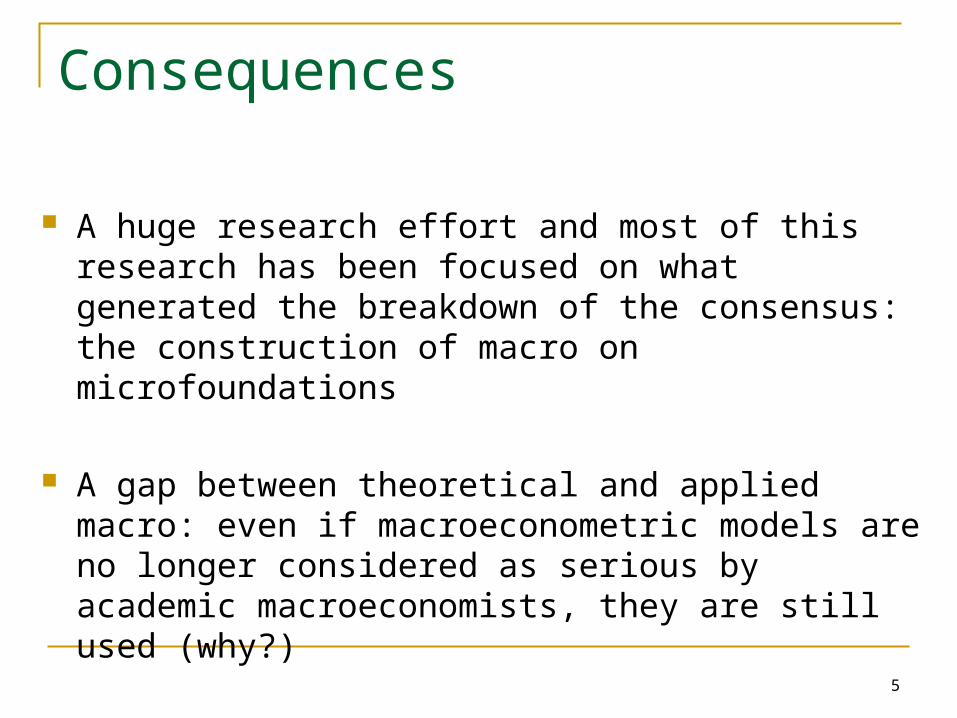
Consequences

A huge research effort and most of this research has been focused on what generated the breakdown of the consensus: the construction of macro on microfoundations

A gap between theoretical and applied macro: even if macroeconometric models are no longer considered as serious by academic macroeconomists, they are still used (why?)

6

Taxonomy of the research efforta. Modelling of expectations

b. New-classical modelling

c. New-keynesian modelling

7

Modelling of expectations

Large acceptance of rational expectations 1/ In monetary policySargent et Wallace (1975)

2/ Rule versus discretion : important question re-examined through rational expectations

3/ Expectations and empirical work, in particular consumption, Hall (1978)

8

New-classical modelling

Optimizing agents

Markets at the equilibrium

9

Imperfect information

Lack of information Produceurs think that the increase in the price only applies to

their products: they believe it is a relative price change and not a general level of price change.

Workers wish to provide more work since they believe that the increase in nominal wage is an increase in real wage

Cycles at equilibrium (Lucas JET 1972, AER 1973 Barro JPE 1978)

BUT : how realistic the assumption of a lack of information about prices?

10

RBC

(Long Plosser, JPE 1983 ; Barro king, QJE 1984).

This theory has 3 strenghts:

(i)  Models are simple

(ii) They are rigorously microfounded

(iii) They do a good job at reproducing the behavior of macro variables.

11

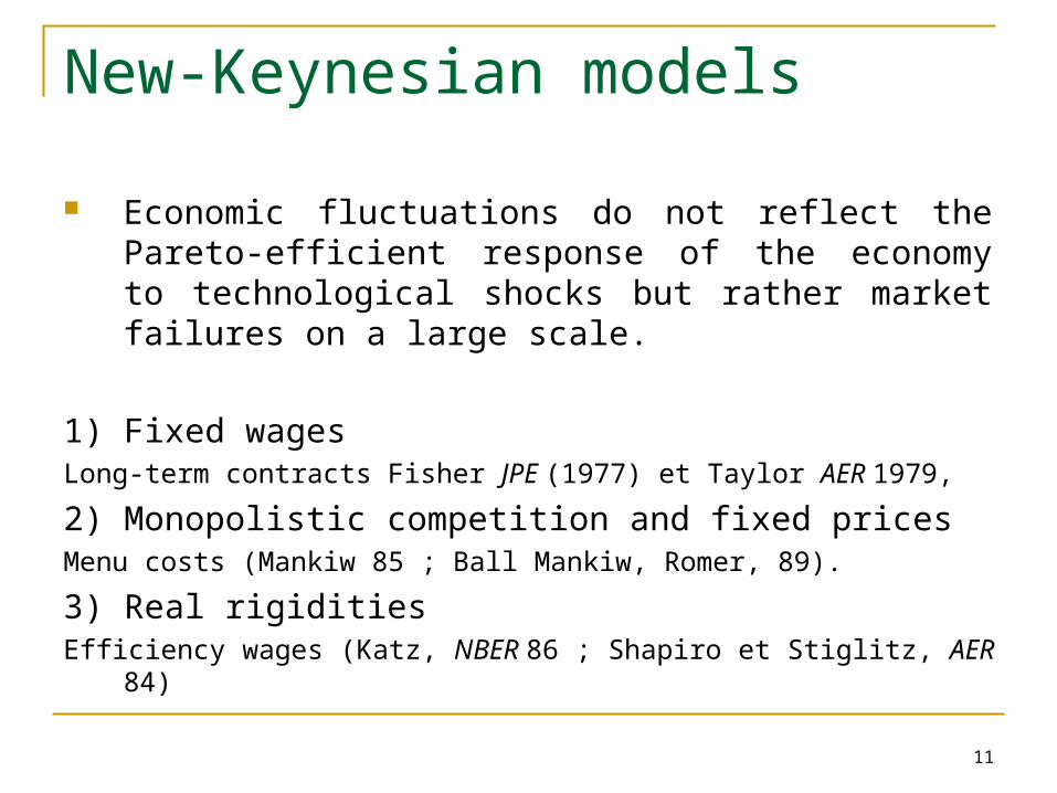
New-Keynesian models

Economic fluctuations do not reflect the Pareto-efficient response of the economy to technological shocks but rather market failures on a large scale.

1) Fixed wagesLong-term contracts Fisher JPE (1977) et Taylor AER 1979,

2) Monopolistic competition and fixed pricesMenu costs (Mankiw 85 ; Ball Mankiw, Romer, 89).

3) Real rigiditiesEfficiency wages (Katz, NBER 86 ; Shapiro et Stiglitz, AER 84)

12

Conclusion

1/ what is largely accepted

2/ no consensus in particular for what concerns the theory of cycles

- New-classical theory

- New-Keynesian theory

13

King and Rebelo (1999) “Resuscitating RBC”"Business cycles research studies the causes and

consequences of the recurrent expansions and contractions in aggregate economic activity"

- Which sources ?- Why cycles ?

→ are BC alike across time and countries ?

2. RBC methodology

14

R. Lucas (1977) «Understanding Business Cycles»“…[understanding] business cycles means constructing a

model in the most literal sense: a fully articulated artificial economy which behaves through time as to imitate closely the time series behavior of actual economies.”

→ the model will be

- in general equilibrium

- microfounded

- dynamic

- stochastic

15

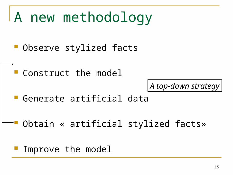
A new methodology

Observe stylized facts

Construct the model

Generate artificial data

Obtain « artificial stylized facts»

Improve the model

A top-down strategy

16

3. Fluctuations and facts

“Business cycles are a type of fluctuation found in the aggregate economic activity of nations that organize their work mainly in business enterprises: a cycle consists of expansions occurring at the same time in many economic activities, followed by similarly general recessions, contractions and revivals which merge into the expansion phase of the next cycle; this sequence of changes is recurrent but not periodic; in duration, business cycles vary from more than one year to ten or twelve years; they are not divisible into shorter cycles of similar character with amplitudes approximating their own.”

Burns and Mitchell [1946]“Measuring business cycles”, NBER

17

BUSINESS CYCLE DURATION IN MONTHSREFERENCE DATESPeak Trough Contraction Expansion CycleQuarterly dates Peak Previous trough Trough from Peak fromare in parentheses to to Previous Previous

Trough this peak Trough Peak

December 1854 (IV) -- -- -- --June 1857(II) December 1858 (IV) 18 30 48 --October 1860(III) June 1861 (III) 8 22 30 40April 1865(I) December 1867 (I) 32 46 78 54June 1869(II) December 1870 (IV) 18 18 36 50October 1873(III) March 1879 (I) 65 34 99 52

March 1882(I) May 1885 (II) 38 36 74 101March 1887(II) April 1888 (I) 13 22 35 60July 1890(III) May 1891 (II) 10 27 37 40January 1893(I) June 1894 (II) 17 20 37 30December 1895(IV) June 1897 (II) 18 18 36 35

June 1899(III) December 1900 (IV) 18 24 42 42September 1902(IV) August 1904 (III) 23 21 44 39May 1907(II) June 1908 (II) 13 33 46 56January 1910(I) January 1912 (IV) 24 19 43 32January 1913(I) December 1914 (IV) 23 12 35 36

August 1918(III) March 1919 (I) 7 44 51 67January 1920(I) July 1921 (III) 18 10 28 17May 1923(II) July 1924 (III) 14 22 36 40October 1926(III) November 1927 (IV) 13 27 40 41August 1929(III) March 1933 (I) 43 21 64 34

Source: Public Information Office National Bureau of Economic Research, Inc.

Business Cycles expansionsand contractions

18

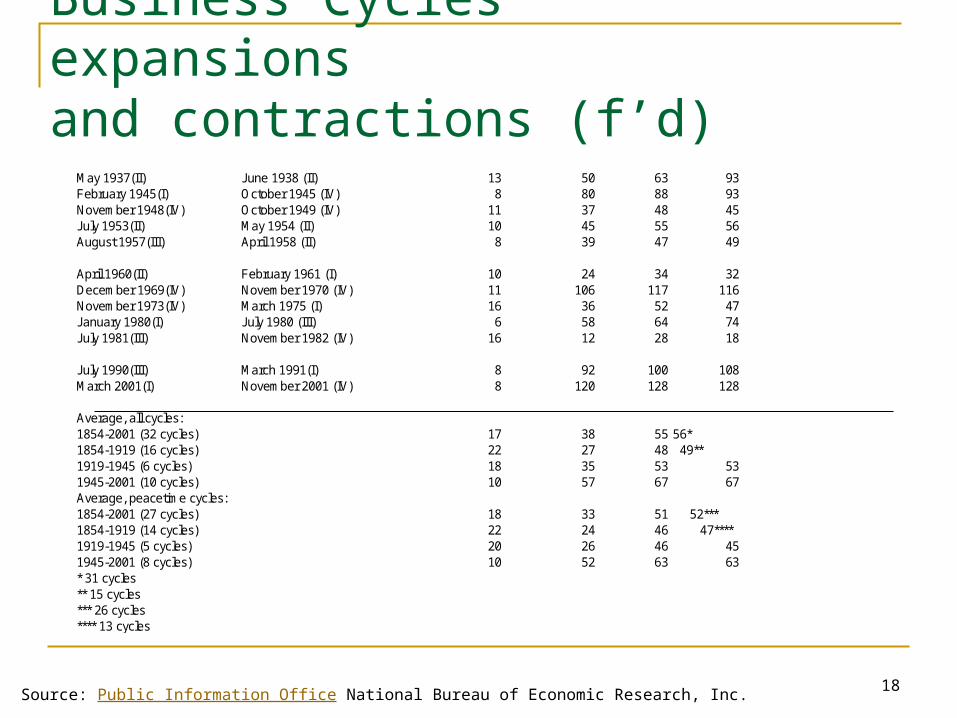
May 1937(II) June 1938 (II) 13 50 63 93February 1945(I) October 1945 (IV) 8 80 88 93November 1948(IV) October 1949 (IV) 11 37 48 45July 1953(II) May 1954 (II) 10 45 55 56August 1957(III) April 1958 (II) 8 39 47 49

April 1960(II) February 1961 (I) 10 24 34 32December 1969(IV) November 1970 (IV) 11 106 117 116November 1973(IV) March 1975 (I) 16 36 52 47January 1980(I) July 1980 (III) 6 58 64 74July 1981(III) November 1982 (IV) 16 12 28 18

July 1990(III) March 1991(I) 8 92 100 108March 2001(I) November 2001 (IV) 8 120 128 128

Average, all cycles:1854-2001 (32 cycles) 17 38 55 56*1854-1919 (16 cycles) 22 27 48 49**1919-1945 (6 cycles) 18 35 53 531945-2001 (10 cycles) 10 57 67 67Average, peacetime cycles:1854-2001 (27 cycles) 18 33 51 52***1854-1919 (14 cycles) 22 24 46 47****1919-1945 (5 cycles) 20 26 46 451945-2001 (8 cycles) 10 52 63 63* 31 cycles** 15 cycles*** 26 cycles**** 13 cycles

Source: Public Information Office National Bureau of Economic Research, Inc.

Business Cycles expansions and contractions (f’d)

19

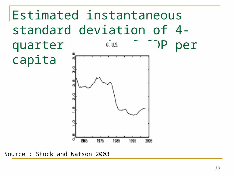
Estimated instantaneous standard deviation of 4-quarter growth of GDP per capita

Source : Stock and Watson 2003

20

Estimated instantaneous standard deviation of 4-quarter growth of GDP per capita (f’ed)

21

22

Stock and Watson (1988)« Variable trends in Economic Time Series »

23

O. Blanchard and S. Fischer [1989] Lectures on macroeconomics“the picture that emerge is […] that of an economy

on which both types of shocks play an important role. Transitory shocks matter and have a hump-shaped effect on output before their effects die out.

But the path of output would be far from smooth even in the absence of those transitory shocks.

What emerges is a more complex image of fluctuations, with temporary shocks moving output around a stochastic trend that itself contributes significantly to the movements in the real GNP”

24

Linear filter 1: HP filter

: cycle component

: trend component

: controls the properties of the trend component generated

by the filter

1

2

2

11

1

2

..

min1

tTTTT

tT

x

xxxxts

xxtT

Tx

J

Jjjj

T xaxxxx ˆ

x

25

King and Rebelo (1999)

26

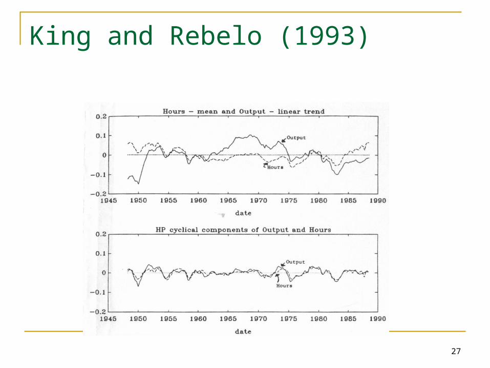
King and Rebelo (1993)

linear

27

King and Rebelo (1993)

28

Stock and Watson (1998)

29

Linear filter 2: BP-filter (Baxter and King, 1999)

The ideal band-pass filter has the following 2-sided infinite moving average representation: :

L : lag operator. Symmetry ( ) is imposed.

For stationary time-series:

: random periodic components

hthth

BPt xLaxax )(

kk aa

dxt )(

)(

30

BP filter (f’d)

Then :

Frequency-response function :

with , and

One can then show that :

dx BPt )()(

otherwise0

if1)(

21

3/,16/ 21 P/2 326 P

,...2,1/)sin(/)sin(/ 12120 hforhhhhaanda h

K

KhtKhth

BKt xLaxax )(

31

M. Baxter and R. King (1999), « Measuring BC: Approximate Band-Pass Filters for Economic Time Series »

32

33

34

Goods’market

35

Inputs

36

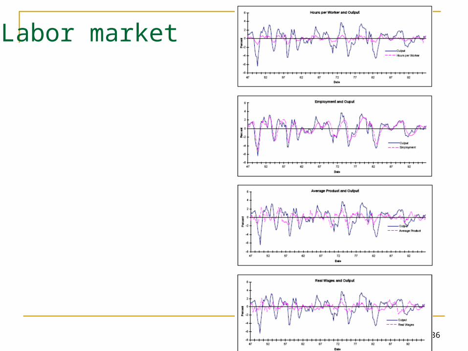
Labor market

37Source: Stock and Watson (1998)

All variables (except r) are in logarithms and have been detrended using HP filter

38

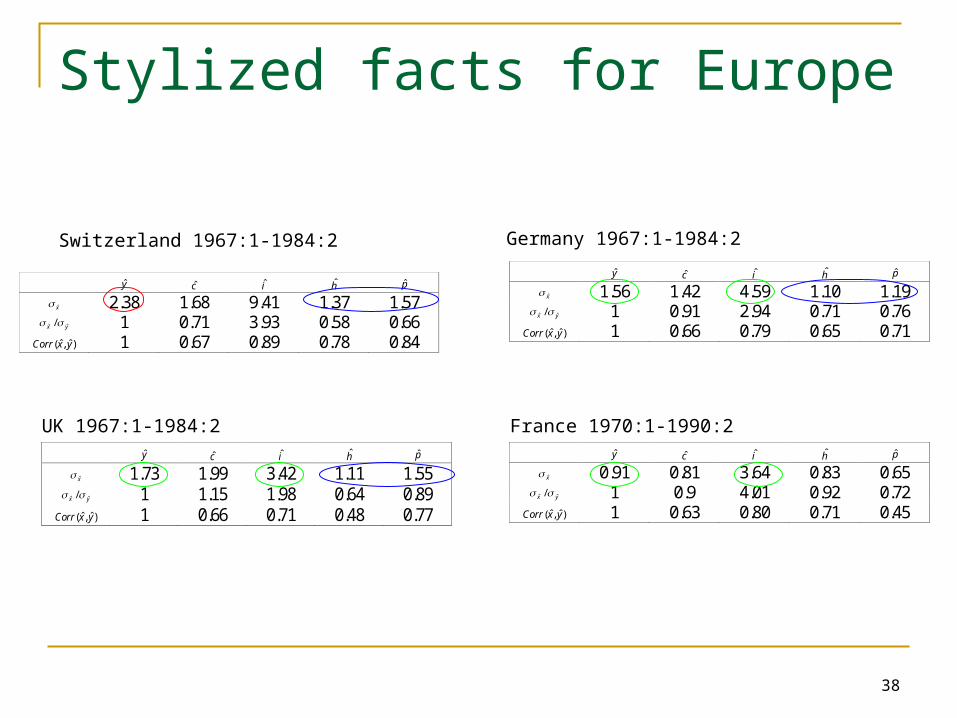
Stylized facts for Europe

y c i h p x 2.38 1.68 9.41 1.37 1.57 yx ˆˆ / 1 0.71 3.93 0.58 0.66

)ˆ,ˆ( yxCorr 1 0.67 0.89 0.78 0.84

y c i h p x 1.56 1.42 4.59 1.10 1.19 yx ˆˆ / 1 0.91 2.94 0.71 0.76

)ˆ,ˆ( yxCorr 1 0.66 0.79 0.65 0.71

y c i h p x 1.73 1.99 3.42 1.11 1.55 yx ˆˆ / 1 1.15 1.98 0.64 0.89

)ˆ,ˆ( yxCorr 1 0.66 0.71 0.48 0.77

y c i h p x 0.91 0.81 3.64 0.83 0.65 yx ˆˆ / 1 0.9 4.01 0.92 0.72

)ˆ,ˆ( yxCorr 1 0.63 0.80 0.71 0.45

Switzerland 1967:1-1984:2 Germany 1967:1-1984:2

UK 1967:1-1984:2 France 1970:1-1990:2