1

Intrinsic flame instabilities in combustors: analytic description of a

1-D resonator model

Mukherjee Nalini Kanta, Shrira Victor

School of Computing and Mathematics, Keele University, UK, ST55BG

e-mail: n.k.mukherjee@keele.ac.uk, Phone number: +44 1782733256

The study is concerned with theoretical examination of thermo-acoustic instabilities in

combustors and focuses on recently discovered ‘flame intrinsic modes’. These modes differ

qualitatively from the acoustic modes in a combustor. Although these flame intrinsic modes were

intensely studied, primarily numerically and experimentally, the instability properties and

dependence on the characteristics of the combustor remain poorly understood. Here we

investigate analytically the properties of intrinsic modes within the framework of a linearized

model of a quarter wave resonator with temperature and cross-section jump across the flame, and

a linear n model of heat release. The analysis of dispersion relation for the eigen-modes of

the resonator shows that there are always infinite numbers of intrinsic modes present. In the limit

of small interaction index n the frequencies of these modes depend neither on the properties of

the resonator, nor on the position of the flame. For small n these modes are strongly damped.

The intrinsic modes can become unstable only if n exceeds a certain threshold. Remarkably, on

the neutral curve the intrinsic modes become completely decoupled from the environment. Their

exact dispersion relation links the intrinsic mode eigen-frequency i with the mode number im

and the time lag : 2 1i im m , where m =0, +/-1. The main results of the

study follow from the mode decoupling on the neutral curve and include explicit analytic

expressions for the exact neutral curve on the n plane, and the growth/decay rate

dependence on the parameters of the combustor in the vicinity the neutral curve. The instability

domain in the parameter space was found to have a very complicated shape, with many small

islands of instability, which makes it difficult, if not impossible, to map it thoroughly

numerically. The analytical results have been verified by numerical examination.

Keywords: Flame intrinsic modes, n model, combustors, flame stability, thermo-acoustic

instabilities.

1. Introduction

Instability in modern day combustors is an issue of fundamental interest and major practical

concern [1]. The need of lowering emissions pushes engineers to create ‘green’ combustion

systems by enhancing combustion efficiency and lowering emission products. In this context

lean premixed pre-vaporized combustors became the most popular way to address this challenge

[2, 3]. The drawback of these combustors is their susceptibility to combustion instability. These

instabilities are thermo-acoustic instabilities that can lead to self-sustained oscillations and cause

severe damage to the combustor. It has been common to assume that thermo-acoustic instabilities

are triggered by the coupling of flame heat release and one of the acoustic modes. The acoustic

modes exist even in the absence of the flame. Thus, the overwhelming majority of studies of

2

combustion instabilities in last few decades was focused on the understanding of the acoustic

modes, e.g. Lieuwen and Yang [4], Poinsot and Veynante [5], Schuller et al. [6] and Dowling et

al. [7, 8].

However, recently, a major shortcoming of the established paradigm has been identified by

Hoeijmakers et al. [9], Hoeijmakers [10] and Bomberg et al. [11]. Hoeijmakers et al. [9]

suggested that the flame subsystem in a combustor can give rise to a completely new family of

modes, which are often referred to as the flame intrinsic-thermoacoustic modes. Although it

would be more appropriate to call them intrinsic thermoacoustic modes of the flame and its

nearby environment (burner). For brevity, throughout the paper we will call them just intrinsic

modes. Thus, a set of intrinsic modes (which might be unstable) can exist in a combustor, apart

from the conventional acoustic modes. Hoeijmakers et al. [9] considered a n combustor

model with gradually varying reflection coefficient at the ends (i.e. +1 to 0 at the closed end and

-1 to 0 at the open end) and numerically evaluated intrinsic mode frequencies. Their analytical

analysis was confined to an infinite system. The implicit dispersion relation for the flame in an

infinite system was found to be, 1 ( ) 0F , where, ( )F is flame transfer function,

is ratio of specific acoustic impedances and is ratio of temperatures across the flame. The real

parts of the intrinsic mode frequencies for an infinite system were found to be 2k ,

where, is time lag and k is an integer. The explicit expressions for the threshold of instability

and the decay rate were given as, 1 and 1 ln 1 n , respectively. The analytical

results were complemented by numerical analysis of a single intrinsic mode in a resonator. A

possible physical explanation of the origin of flame intrinsic modes was suggested to be the

flame reaction on the acoustic velocity fluctuations, created by its own heat release fluctuation.

In other words, the flame (and its nearby environment) might create its own local, potentially

unstable, feedback loop. Independently, Bomberg et al. [11] performed theoretical stability

analysis using scattering matrix of the flame and matched their results with experiments

(Gentemann and Polifke [12], Kaess et al. [13]) for two combustor setups, one with a laminar

flame holder stabilized and another with swirl stabilized turbulent flame. Thermo-acoustic

instabilities observed in these combustor setups were interpreted as manifestations of intrinsic

flame instability. Thus, it was concluded that the common assumption that in thermo-acoustic

instabilities flame heat release always locks onto one of the acoustic modes, needs to be critically

reconsidered on a case by case basis. In a parallel study by Emmert et al [14], the stability of

intrinsic modes was investigated from the viewpoint of a balance of the acoustic energy across

the flame. Direct numerical simulations (DNS) by Courtine et al. [15], Courtine et al. [16] and

Silva et al. [17], where a flame placed in an acoustically anechoic environment, have also

confirmed that the intrinsic thermo-acoustic feedback is a genuine physical phenomenon, and not

just a spurious by-product of simplistic models. Recent study by Emmert et al. [18] has shown

that a sum of acoustic and intrinsic modes constitutes the complete set of eigen-modes of a

combustor. A numerical procedure has been developed to compute the acoustic and intrinsic

eigen-modes of a combustor. It was noted that it is sometimes difficult to distinguish the intrinsic

and acoustic modes, solely, by comparing their mode shapes. It has also been found that

increased acoustic losses at the end of combustor may destabilize the combustion system due to

3

intrinsic flame instability. A somewhat similar observation has been made in experimental study

by Hoeijmakers et al. [19]. The experiments suggest that as the acoustic reflections at the

combustor boundaries decrease, the eigen-frequencies of the system becomes fully determined

by intrinsic flame modes. The possible explanation was given as: the decrease in upstream and

downstream acoustic reflections can put the flame in an open-loop, resulting in exposure of

intrinsic instability properties of the flame.

Once the reality of the intrinsic modes has been established beyond any doubt, the following

natural questions come to the fore. It would be highly desirable to have an analytical criterion on

the appearance of unstable intrinsic modes in a combustor and also, it is important to know the

boundaries and topology of the instability domain in the multi-dimensional parameter space of a

combustor. Besides, the effects of the combustor properties (e.g., flame location, boundary

conditions at the ends, and parameters of the cross-section and temperature jumps) on the

intrinsic mode growth rates and positions have to be studied. To grasp the stability behavior of

intrinsic modes in a multi-dimensional parameter space via numerics might be extremely time

consuming, if not impossible. We reiterate that at present all analytical results for intrinsic modes

are confined to anechoic environment, only. Overall, an integrated picture of the instabilities of

acoustic and intrinsic modes is needed. The present work addresses this need by focusing on the

intrinsic mode part of the picture.

Here we consider a standard 1-D acoustic model of a closed-open combustor with a heat source.

The heat release rate is modeled by the linear n law [20]. Within the framework of this

simplified model we provide an overall picture of the intrinsic modes and explicit analytical

expressions for the parameters of the intrinsic modes (growth rates, neutral curves, frequencies

of unstable modes) for the whole range of the system parameters. We also show that whatever

are the properties of the combustor, including the end conditions, there is always infinite number

of intrinsic modes present. For small n , we derive explicit universal dispersion relation for

intrinsic modes. These modes strongly decay for small n , which makes them practically

impossible to observe. In closed-open combustors these modes can become unstable with

increase of n . The main discovery is that on the neutral curve the transcendental dispersion

relation can be factorized. We call this phenomenon decoupling. Factorization means that the

intrinsic modes become completely decoupled from the environment, i.e. it does not feel the

properties of the combustor. This allows us to treat this problem analytically and to derive all the

characteristics of intrinsic mode instabilities. The instability domain in multi-dimensional

parameter space proved to be so complicated that it would have been close to impossible to

retrieve it numerically.

The paper is organized as follows. In §2 we introduce our model of a quarter wave resonator

with n model of heat release and derive a dispersion relation for small amplitude

oscillations. The dispersion relation takes into account the effects of cross-section and

temperature jumps across the flame. It forms the basis of the subsequent analysis. In §3, for the

sake of completeness, we reproduce the results from Mukherjee et al. [21] and derive an

analytical expression for the intrinsic modes in the limit of small interaction index, n. In this limit

the intrinsic modes are heavily damped. Their frequencies are described by the same analytical

expression as for the case of an infinite tube found by Hoeijmakers et al. [9]. The distinctive

4

features of acoustic and intrinsic modes are also highlighted and discussed using numerical

results. In §4 we describe decoupling of the intrinsic modes from their environment on the

neutral curve and exploit it to derive explicit analytical expressions for the exact intrinsic mode

neutral curve, separating stability/instability domains on the n plane and the growth rate

near the neutral curve. We also find exactly the intrinsic mode frequencies on the neutral curve.

The analytical results are then compared with numerical simulations within the framework of the

dispersion relation obtained in §2 and a very good agreement is demonstrated. In §5 we examine

the dependence on parameters (location of the flame, the cross-section and temperature jump) of

the intrinsic modes. Finally, in §6, we summarize our progress in understanding of intrinsic

modes in a combustor and outline the remaining open questions.

2. 1-D mathematical model of a resonator Throughout this paper we will focus on analytical study of flame intrinsic modes in a

common 1-D model of acoustic quarter wave resonator. The previous analytical studies by

Hoeijmakers et al. [9] were performed for a tube with anechoic boundary condition. The results

of the only earlier analytical study of intrinsic flame modes by Mukherjee et al. [21] will be

reproduced in the next section. The acoustic modes in a resonator were extensively studied (see

e.g., Lieuwen T., and Yang V. [4]). Here we adopt the basic acoustic model from Schuller et al.

[6]. The analytical approach we put forward here can be extended to more complicated

combustor setups, as well. However, for simplicity, we will restrict the current analysis to the

simplest case of a quarter wave resonator. The 1-D analytical formulation based upon n

model provides an efficient versatile tool enabling us to analyze the combustor modes and gives

us a valuable insight into the stability behavior of these modes in multi-dimensional parameter

space.

Figure 1 provides a schematic sketch of a quarter wave resonator with a compact heat

source at qx x , with x being the longitudinal coordinate with the origin at the closed end of

the resonator. 1A , 2

A / 1B , 2

B are the pressure amplitudes for the forward/backward going waves

in the upstream and the downstream region, respectively. The mean temperature is assumed to

jump from 1T to 2

T across the flame. The cross sectional area jumps across the flame from 1S

to 2S . The effect of mean flow is neglected in this analysis.

5

Figure 1: Schematic sketch of a combustor with closed-open end conditions. The combustor has

a cross sectional area jump at the flame location qx x . Thick arrows (brown online) symbolize

the forward/ backward travelling waves upstream/downstream of the flame. Shaded region

(yellow online) marks the domain of higher temperature after the temperature jump across the

flame.

The acoustic pressure and particle velocity at the upstream region and at the downstream region

of the combustor can be written as (e.g., [22]):

1 11 1 1,

ik x ik x i tp x t Ae B e e

, 1

1 1

1 11 1

1,

ik x ik x i tu x t

cA e B e e

, and (1)

2 22 2 2,

ik x ik x i tp x t A e B e e

, 2 2 2

2 2

2 21

,ik x ik x i t

u x t A e B e ec

. (2)

The wave numbers i

k ( i =1,2) upstream and downstream of the flame can be presented as

1 1k c and

2 2k c , where is the complex frequency, 1

c , 2c represents the speed of

sound and 1 , 2

are the mean densities upstream and downstream of the flame, respectively.

We assume ideal boundary conditions at two ends,

at 0x , 1 1 1 0 1A B R , and,

at x L 2 2 2 1ikL ikLB e A e R L . (3, 4)

The pressure and flow rate balance at q

x x implies (Dowling et al. [7], Bauerheim et al. [23]),

1 2

p x p x , and 2

1 1 1 1 2 21S u x c Q S u x . (5, 6)

Here, ( )Q t is the heat release rate at q

x x and represents the ratio of specific heats of air (

p vc c ). It is assumed that the heat source acts like a monopole with a volume outflow

2

1 11 Q c . The linear heat release law can be assumed to be of the form, (see e.g., Truffin

and Poinsot [24])

6

2

1 1 1 11Q t S c nu t . (7)

Here, n and are the interaction index and time lag, respectively. The rate of heat release

fluctuations, Q , is assumed to be proportional to the local velocity upstream of the flame, 1u ,

with a time lag, . In the frequency domain this can be written as,

2

1 1 1 11 iQ S c ne u . (8)

The set of homogeneous equations for 1A , 1

B , 2A and 2B , (3)-(6) is usually presented in the

matrix form (e.g., Schuller et al. [6])

1 1 2 2

1 1 2 2

2 2

2 1 1 2 1 1

1 2 2 1 2 2

1

1

2

2

1 1 0 00

0

01 1

00 0

q q q q

q q q q

ik x ik x ik x ik x

ik x ik x ik x ik xi i

ik L ik L

S c S c

S c S c

Ae e e e

B

Ane e ne e e e

Be e

.

(9)

For a nontrivial solution of the eigen-value problem (9) to exist the determinant D of the 4 4

matrix in (9) has to be zero, which yields D=0. Here we, however, find it more convenient to use

a compact dispersion relation

2 1 1 2

2 1 1 2

1 2 2 1 2

1 2 2 1 2 1 2

1 cos

1 cos 2 sin sin 0

q

q q q

i

S S c c

S S c c

k k x k L

k L k k x ne k x k x L

. (10)

This compact form of dispersion relation provides the basis of all analytical derivations in the

subsequent sections. We denote the function on the left hand side of transcendental equation (10)

as f . Thus, dispersion relation (10) can be re-written compactly as,

0f . (11)

The dispersion relation can be simplified for special cases worth considering in detail. When

there is no cross-section and temperature jumps across the flame, that is 1 2

S S and 1 2

T T ,

and thus 1 2

c c , 1 2 and

1 2k k k , dispersion relation (10) reduces to

cos sin sin 0q q

ikL ne kx k x L

. (12)

The dispersion relation (12) can be further simplified, when the flame is located exactly in the

center of the resonator, i.e. at 2q

x L ,

cos 2i i

kL ne ne

. (13)

The dispersion relation (10), (12) and (13) prescribes the eigen-frequencies of the system in

implicit form. Equation (10) describes the most general case (a quarter wave resonator with a

cross-section and temperature jump across the flame), while equations (12) and (13) are the

7

reduced versions of (10) for special cases. The real part of is the frequency and the imaginary

part is the growth/decay rate. Since the dispersion relation in the form (10) is more amenable for

analytical study than the commonly used matrix formulation (i.e. the determinant of the 4 4

matrix in equation (9), equated to zero), we employ it as the starting point for our subsequent

analysis. For an insight into the physics of flame intrinsic modes, the particular simplifications of

the dispersion relation (12), (13) will be also used. There is no general method enabling one to

solve transcendental equations of this type. However, as we show in §4, the dispersion relation

can be factorized on the neutral curves, which allows us to find the neutral curve exactly and

approximate solutions in its vicinity.

3. The place of intrinsic modes in the general picture of the

resonator modes

In this section for completeness we reproduce the results of the analytical study of flame intrinsic

modes in a 1-D resonator from Mukherjee et al. [21]. We derive analytical expressions for

intrinsic mode frequency and decay rate in the limit of small n and numerically validate the

formula.

3.1. Analytical expression for intrinsic modes in the limit of small n for

arbitrary end conditions

To fix the idea we start with the simplest form of dispersion relation, namely, (13), which

provides an implicit expression for all the modes present in the resonator. The presence of flame

intrinsic modes, different from the conventional acoustic modes, has been established recently

[9]. Both stable and unstable intrinsic modes were observed in experiments and simulations, e.g.

[11, 16, 17]. The unstable modes seemingly appear out of nowhere. To understand better the

place of intrinsic modes in the big picture it is desirable to know whether these modes exist when

they are not unstable, and if yes, where in the complex plane are their frequencies. In this section

we address these questions for the case of a quarter wave resonator in the limit of weak flame.

From the simplified dispersion relation (13) it is easy to see that for 0n there are only two

sets of roots:

(i) the conventional acoustic modes specified by condition cos 0kL , and,

(ii) a new set of roots with large negative imaginary part (this is, |i

e

|>>1, or, in other

words, the strongly damped modes). This can be explained as follows. For nonzero coskL , there

is only one possibility for equation (13) to have solutions, that is the numerator has to be (1)O .

This implies that when n is small, i

e

has to be large. We now apply the same reasoning to the

general case.

The dispersion relation can be derived for generic combustors with arbitrary 1

0R and 2

R L

retained in the original form in equations (3) and (4), it reads

8

1 1 2 2

1 2 2 1

1 2 2 1

2 1 1 2

1 0 1 0

0 0 0

ii i i i

i i i i

R R L R L R

R L R R R L

e e e e ne

e e e e

. (14)

where , 1 and 2 are given by,

2 1 1

1 2 2

S c

S c

, 2 1 2

1

1 1q

L

c c cx

and 2 1 2

2

1 1q

L

c c cx

. (15)

To find the roots of the general dispersion relation (14) in the limit of small n we multiply both

sides of the resulting equation by

1ie . This leads to the following expression,

1 2 1 21

1 2 1 21

1 2 2 1

2 1 1 2

2

2

1 0 1 0

0 0 0

ii ii

i ii

R R L R L R

R L R R R L

e e e ne

e e e

. (16)

By the same reasoning (as for the simplified dispersion relation considered above), the new set of

roots (intrinsic modes) for the general dispersion relation (14) must have large negative

imaginary part. Thus, for these new roots all the exponents in (16), (that is 12i , 1 2i

and

1 2i

) contain highly negative real part, as well. Hence, for small n , 12

0i

e

,

1 2 0i

e

, 1 2 0

ie

. Then dispersion relation (16) reduces to the following simplified

form that exhibits decoupling of intrinsic modes from the combustor end conditions 1

0R and

2

R L ,

1 21 0 0ine R R L . (17)

Equation (17) shows that in the limit of small n intrinsic modes are so localized, that they do not

feel the acoustic boundaries. Equation (17) leads us to an explicit dispersion relation for intrinsic

modes in the limit of small n , valid for any 1-D combustor obeying n model of flame heat

release,

1 0ine . (18)

Equation (18) generates the explicit solution for intrinsic mode frequency in the asymptotic limit

of small n , as follows,

2 1 ln 1 2 1 lni im i n m i n . (19 a,b)

where, im is the mode number of the flame intrinsic modes. If we assume the cross-section to be

constant, then expression (19a) is identical to the result found by Hoeijmakers et al. [9] for an

infinite tube with a flame inside. Note a difference in notation: in the present paper n is the same

as in Courtine et al. [16], which relates to n in Hoeijmakers et al. [9] (here labeled as Hn ) as

Hn n , where 2 1 1T T . Thus, in the limit of small n intrinsic modes for 1-D resonator

have the same frequencies as those in infinite tube. We stress that the frequencies given by (19b)

9

do not depend on any parameters of the resonator including the end conditions. Note, that the

intrinsic modes have their own mode numbers, completely independent of the mode numbers of

the acoustic modes.

From equation (19b) it is also easy to see that in the limit of small n there is always infinite

number of intrinsic modes present in the system for any n and . The real part of the flame

intrinsic mode frequency depends only on the time lag alone and is given by the expression,

2 1i

m . The decay rates, however, do not depend on the mode number (im ). Decay

rates are inversely proportional to and logarithmically depend on n and the temperature and

cross-section jumps of the resonator. In the asymptotic limit of small n , flame intrinsic modes

are always strongly damped and independent of the characteristics of the resonator and flame

position. Since the decay rate is high, the intrinsic modes to leading order in 1ik L

e

do not feel

the combustor boundaries. This explains why the result coincides with those for the infinite tube.

The practical implication of strong damping of the intrinsic modes in combustors with weak

flames is that this feature makes it practically impossible to observe their manifestations in such

regimes. Intrinsic modes could only be visible when flame heat release rate is high enough for

these modes to approach the neutral curve. In § 4.2 we derive an explicit criterion for occurrence

of intrinsic mode instability in the closed-open combustors.

Thus, for small but nonzero n there is always infinite number of flame intrinsic modes present in

a combustor, just like there is infinite number of acoustic modes present in a resonator. However,

in contrast to nearly neutral acoustic modes, for small n all these modes are strongly damped.

They cease to exist for n =0, while acoustic modes do not. We have established that in the limit

of small n these modes are equally spaced and their frequencies are determined only by the time

lag and, correspondingly, do not depend at all on other characteristics of the system. We will

show below that in certain bands of the intrinsic modes can become unstable when the value

of n exceeds certain threshold. Their behavior in the vicinity of neutral curve will be studied in §

4. In itself the dispersion relation behavior in the limit of small n is important only in the context

of outlining the general picture of intrinsic modes. But its significance becomes apparent in § 4,

since the frequencies of intrinsic modes on the neutral curve prove to coincide exactly with the

real parts of the eigen-values found in the small n limit.

3.2. Understanding the stability behavior of intrinsic modes

Here we examine the features of the full dispersion relation (10) numerically. For certainty, we

consider as an example a combustor with the parameters of the test rig at IIT Madras (Vishnu et

al. [25]): the length L is 0.75 m, the cross-section S is 0.0016 m2 (based on 45 mm inner

diameter of the lab scale combustor setup), the temperature T is constant throughout the duct and

equal to 297 K when there is no flame.

10

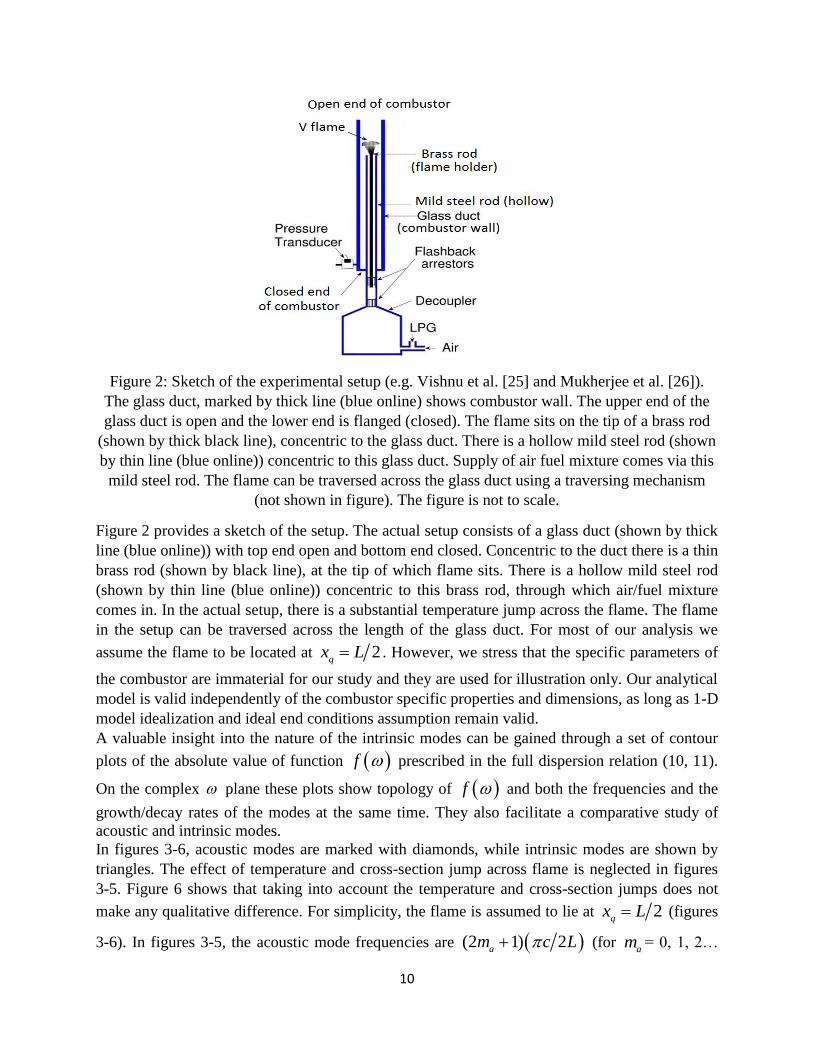
Figure 2: Sketch of the experimental setup (e.g. Vishnu et al. [25] and Mukherjee et al. [26]).

The glass duct, marked by thick line (blue online) shows combustor wall. The upper end of the

glass duct is open and the lower end is flanged (closed). The flame sits on the tip of a brass rod

(shown by thick black line), concentric to the glass duct. There is a hollow mild steel rod (shown

by thin line (blue online)) concentric to this glass duct. Supply of air fuel mixture comes via this

mild steel rod. The flame can be traversed across the glass duct using a traversing mechanism

(not shown in figure). The figure is not to scale.

Figure 2 provides a sketch of the setup. The actual setup consists of a glass duct (shown by thick

line (blue online)) with top end open and bottom end closed. Concentric to the duct there is a thin

brass rod (shown by black line), at the tip of which flame sits. There is a hollow mild steel rod

(shown by thin line (blue online)) concentric to this brass rod, through which air/fuel mixture

comes in. In the actual setup, there is a substantial temperature jump across the flame. The flame

in the setup can be traversed across the length of the glass duct. For most of our analysis we

assume the flame to be located at 2q

x L . However, we stress that the specific parameters of

the combustor are immaterial for our study and they are used for illustration only. Our analytical

model is valid independently of the combustor specific properties and dimensions, as long as 1-D

model idealization and ideal end conditions assumption remain valid.

A valuable insight into the nature of the intrinsic modes can be gained through a set of contour

plots of the absolute value of function f prescribed in the full dispersion relation (10, 11).

On the complex plane these plots show topology of f and both the frequencies and the

growth/decay rates of the modes at the same time. They also facilitate a comparative study of

acoustic and intrinsic modes.

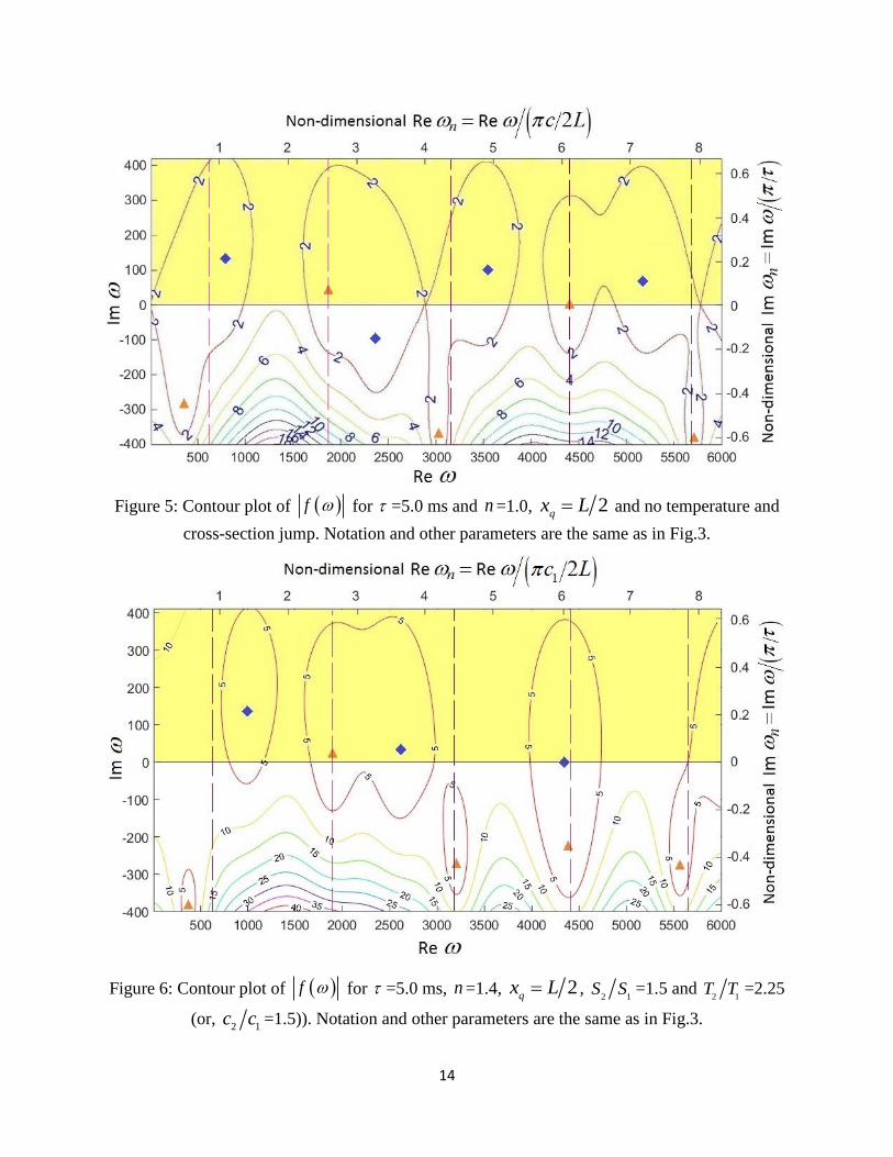
In figures 3-6, acoustic modes are marked with diamonds, while intrinsic modes are shown by

triangles. The effect of temperature and cross-section jump across flame is neglected in figures

3-5. Figure 6 shows that taking into account the temperature and cross-section jumps does not

make any qualitative difference. For simplicity, the flame is assumed to lie at 2q

x L (figures

3-6). In figures 3-5, the acoustic mode frequencies are (2 1) 2a

m c L (for a

m = 0, 1, 2…

11

and assuming 1c = 2

c = c ) [27] and have zero growth rates in figure 3. The instability domain is

lightly shaded (marked in yellow online). The iso-lines in the figures 3-6 present the mapping of

the absolute value of f onto the complex plane. The innermost closed loops of the iso-

lines represent the solution region for modal frequency . In figures 3-5, the real part of

frequencies of the modes are given both in dimensional form ( in rad/s) and, in parallel, non-

dimensionalized on the fundamental modal frequency of acoustic mode ( 2c L in rad/s), i.e.

Re Re 2n c L . In figure 6, the non-dimensionalization is performed by cold

resonator frequency of acoustic mode (1 2c L in rad/s). The growth rate is non-

dimensionalized by intrinsic instability frequency, i.e. Im Imn . The number

of frequencies in the system, indeed, exceeds by far the number of acoustic modes, as was also

noted by Emmert et al. [18] in their analysis of a premixed combustor.

To show in the same figure the iso-lines of f for both acoustic and intrinsic modes with

huge difference in the decay rates, we split figure 3 into two panels: for small interaction index

n ( n =0.025) and time lag, equal to 3 ms. In the chosen frequency range there are three

intrinsic modes with strong decay rates, as shown in the bottom panel. These modes are equally

spaced and the frequencies of these modes are well predicted by (19a). The upper panel shows

acoustic modes, which are neutral for the chosen n and . When in figure 4, n is increased

from 0.025 to 1.0, this decreases significantly the decay rates of the intrinsic modes.

Comparison of figures 4 and 5 shows that increase of from 3 ms to 5 ms reduces the intrinsic

mode frequency. At some threshold value of n these intrinsic modes become unstable. For

example, the fourth intrinsic mode at 4398 rad/s becomes unstable when n is 1.0. This instability

frequency is the same frequency as predicted by equation (19a) in the asymptotic limit of small

n . The same is true for the second intrinsic mode. This behavior of intrinsic instability frequency

(being the same as in the limit of small n ) is robust: it does not depend on the presence of

temperature or cross-section jumps in the system, as illustrated by figure 6, where temperature

and cross-section jump across the flame are taken into account. Even in this case the second

intrinsic mode attains instability at the same frequency as predicted by equation (19a) in the

asymptotic limit of small n . However, this is not the only possibility. In § 4.1, we will show that

the intrinsic modes can also attain instability at a frequency shifted by with respect to the

frequency 2 1i

m predicted by equation (19a). The intrinsic mode frequency might also

shift for the modes remaining linearly stable for all n , e.g. the first intrinsic mode in figures 4, 5.

Numerical simulations (not shown here) indicate that in certain bands of all intrinsic modes

become unstable upon exceeding certain n -threshold, the threshold will be derived analytically

in § 4.2.

In summary, we can say that intrinsic modes are strongly damped in the limit of small n and in

this range are easily distinguishable from acoustic modes. On the complex plane the modes

could be always distinguished by tracing their position by varying n . The frequency of the

12

intrinsic modes depends primarily on and does not depend on any parameters of the combustor

(within the framework of the adopted model of the closed-open combustor with ideal end

conditions). We stress that the frequency depends on n very weakly. In contrast, the intrinsic

modes stability is strongly dependent on n . These modes can become unstable upon exceeding a

certain threshold value of n .

13

Figure 3: Contour plot of f for n =0.025 and =3.0 ms for the particular case 2q

x L

and no temperature and cross-section jump. The parameters used for this plot are: the length L

is 0.75 m, the cross-section S is 0.0016 m2, the temperature T is constant throughout the duct and

equal 297 K ( 1c = 2

c = c =345 m/s). Two sections are parts of the same contour plot. The domain

of instability is lightly shaded (marked in yellow online). Diamonds (blue online) and triangles

(orange online) represent the acoustic and intrinsic modes, respectively. Dashed vertical lines

indicate the intrinsic mode frequency in the limit of small n , given by equation (19a).

Figure 4: Contour plot of f for n =1.0, =3.0 ms. Notation and other parameters are the

same as in Fig 3.

14

Figure 5: Contour plot of f for =5.0 ms and n =1.0, 2q

x L and no temperature and

cross-section jump. Notation and other parameters are the same as in Fig.3.

Figure 6: Contour plot of f for =5.0 ms, n =1.4, 2q

x L , 2 1

S S =1.5 and 2 1

T T =2.25

(or, 2 1

c c =1.5)). Notation and other parameters are the same as in Fig.3.

15

3.3. Maps of acoustic and intrinsic modes on the n plane

The similarities and the differences between acoustic and intrinsic modes can also be elucidated

by a set of maps on the n plane. These maps offer us a lucid picture of the evolution of

intrinsic modes in the parameter space and also serve as a validation tool for our analytical

results of §3.1. Figures 7 and 8 give examples of such kind of maps for acoustic and intrinsic

modes. The acoustic modes are indicated by squares and intrinsic modes by circles. These modal

frequencies are tracked down manually on the complex frequency plane (as shown in contour

plots 3-6) by changing parameters n and . The numerical results are compared with the

analytical solution (19a) for small n . The effect of temperature and cross-section jump is

neglected here (and thus, 1c = 2

c = c =345 m/s) and the flame is assumed to lie at 2qx L . In

parallel with the dimensional time lag we also use a non-dimensional time lag, 2n

c L

employing the natural acoustic mode timescale 2L c , where c is the sound speed in the absence

of temperature jump. When the fundamental frequencies of acoustic mode ( am =0) and the

intrinsic mode (im =0) are the same, i.e. 2c L , this will correspond to 1

n . Modal

frequencies of intrinsic modes are given both in dimensional form ( f in Hz) and, in parallel,

non-dimensionalized on the fundamental modal frequency of acoustic mode ( 4c L in Hz), i.e.

4nf f c L .

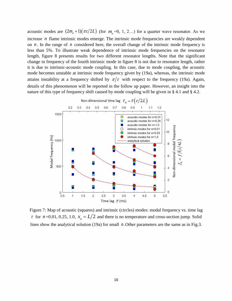
In figure 7 the time lag varies from 1 ms to 5 ms. Three different values of n are considered:

n = 0.01, 0.25 and 1.0 and the corresponding modal frequencies are obtained using contour plots.

The flame intrinsic mode frequencies have (1/ ) dependence well outside the limit of small n ,

which is shown by solid line hyperbolae, representing the analytical solution (19a) for small n .

Multiple hyperbolic lines arise from the same analytical equation (19a). For example, in figure 7

we find that for time lag of 1, 2, 3, 4 and 5 ms, as per equation (19a) the first intrinsic mode

frequencies are 500 Hz, 250 Hz, 166 Hz, 125 Hz and 100 Hz, respectively. These frequencies are

connected by the lowest hyperbolic line. Similar exercise is carried out for higher order intrinsic

modes, as well. Recall, that the squares and circles in figures 7-8 indicate exact solutions of the

full dispersion relation (10) corresponding to the acoustic and intrinsic modes respectively. In the

range of small n it is easy to distinguish the acoustic and intrinsic modes. The key implicit

assumption employed in drawing these figures is that that the modes identified as acoustic

(intrinsic) for small n remain acoustic (intrinsic) when n is increased. This assumption is not

always justified. Coupling of acoustic and intrinsic modes might switch identities, i.e. in figures

7-8 the circles (intrinsic modes) and the nearby squares (acoustic modes) might swap positions.

This effect is ignored in figures 7-8. Here we did not carry out an extra analysis required to

establish whether a particular mode remains acoustic for a chosen value of n . Detailed

discussion of this phenomenon will be reported in the follow up paper.

In figure 8, is fixed at 5 ms and n is varied from 0 to 1.5. The corresponding modal

frequencies are obtained from the contour plots similar to figures 3-6. When flame is not present

in the system, (that is, 0n ), the intrinsic modes are absent, while the frequencies of the

16

acoustic modes are (2 1) 2am c L (for a

m =0, 1, 2…) for a quarter wave resonator. As we

increase n flame intrinsic modes emerge. The intrinsic mode frequencies are weakly dependent

on n . In the range of n considered here, the overall change of the intrinsic mode frequency is

less than 5%. To illustrate weak dependence of intrinsic mode frequencies on the resonator

length, figure 8 presents results for two different resonator lengths. Note that the significant

change in frequency of the fourth intrinsic mode in figure 8 is not due to resonator length, rather

it is due to intrinsic-acoustic mode coupling. In this case, due to mode coupling, the acoustic

mode becomes unstable at intrinsic mode frequency given by (19a), whereas, the intrinsic mode

attains instability at a frequency shifted by with respect to the frequency (19a). Again,

details of this phenomenon will be reported in the follow up paper. However, an insight into the

nature of this type of frequency shift caused by mode coupling will be given in § 4.1 and § 4.2.

Figure 7: Map of acoustic (squares) and intrinsic (circles) modes: modal frequency vs. time lag

for n =0.01, 0.25, 1.0, 2q

x L and there is no temperature and cross-section jump. Solid

lines show the analytical solution (19a) for small n .Other parameters are the same as in Fig.3.

17

Figure 8: Map of acoustic (squares) and intrinsic modes (circles): modal frequency vs.

interaction index n . Solid lines show analytical solution (19a) for small n . The plot is for: =5

ms and two different resonator lengths: L = 0.75m, 0.375m. The flame is at 2

qx L and there

is no temperature and cross-section jump. The first, second, third, fourth and fifth intrinsic modes

are indicated by numbers (i), (ii), (iii), (iv) and (v), respectively.

Crucially, the analytical prediction of the intrinsic mode frequencies (19a) obtained in the

asymptotic limit of small n is found to be a very good approximation for a wide range of n . A

substantial variation of n hardly alters the intrinsic mode frequencies when we have intrinsic

mode instability. However, a significant shift of frequency can be visible when we have intrinsic-

acoustic mode coupling (e.g. the fourth intrinsic mode in figure 8) or when intrinsic mode

remains linearly stable for all n (e.g. the first intrinsic mode in figure 8). The detailed discussion

is beyond the scope of current paper. The intrinsic mode frequency shift by with respect

to the frequency (19a) will be explained in § 4.1.

4. Intrinsic mode instability: neutral curves and growth rates Hoeijmakers et al. [9] found intrinsic modes to be unstable for some values of n and . Small n

limit of dispersion relation (19b) also suggests that the decay rate of intrinsic modes is

logarithmically dependent on n . As n increases, the decay rate decreases and at some threshold

value of n , the decay rate crosses zero, making the intrinsic mode unstable. Here, in §4.1, we

will derive exact analytical expression for the intrinsic mode frequency at the neutral curve.

Then, in §4.2, will find the exact threshold value of n for intrinsic mode instability, that is, we

will find the neutral curve in the n parameter space. In §4.3 we derive the growth/decay

rates near the neutral curve. The geometry of instability domains for each mode proved to be

18

quite complicated. Hence, to simplify handling of infinite number of modes we introduce bounds

for the stability domain in §4.4 and derive simple estimate of the largest growth rate in §4.5.

4.1. The frequency of the intrinsic modes at the neutral curve

In the previous section we have found the intrinsic mode frequency in the limit of small n . Here

we derive the exact frequency at the neutral curve on the n plane taking into account cross-

section jump, temperature jump and flame location.

4.1.1. Decoupling on the neutral curve

The intrinsic modes found analytically for small n can be traced numerically for arbitrary n . At

first, we denote by c

i the discrepancy between the eigen-frequency i and 0

i , the small n

prediction given by real part of (19a). We, however, stress that we do not a priori assume

0c

i i to be small in our analysis. Thus, for any n , 0

i

c

i iRe , where superscript i

denotes the intrinsic modes. For any value of n the intrinsic mode frequency can be written

as, i i iRe iIm , or 0 c

i i ii iIm . On substituting this presentation of

i into the full dispersion relation (10), we can re-write it as,

1 2

0 0

0

0 0

1 21 cos 1 cos

2 sin sin 0q q

c c

i i ic

c c

i i

i i

i i i i

i iImi i i ix c x L c

iIm iIm

ne iIm iIm

,

(20)

where , 1 and 2 are given by equation (15). By virtue of real part of (19a) we have,

0 1ii

e

. Substitution of this identity into (20) simplifies it further. By definition, iIm is

equal to zero for the threshold value of n , i.e. 0iIm at th

in n . This specifies the neutral

curve. Thus, on the neutral curve the imaginary part of (20) reduces to,

1 22 sin sin sin 0

q qcth

i iin k x k x L . (21)

Thus, this equation becomes factorized. It is satisfied when just one multiplier containing c

i

vanishes, that is,

sin 0c

i . (22)

This gives us an explicit expression for c

i ,

c

i m , (23)

where m is an integer (not to be confused with the intrinsic mode number im ). Once c

i is

obtained via (23), the frequency for neutral intrinsic mode can be calculated using its definition

0

i

c

i iRe , which yields (on the neutral curve i iRe ),

19

2 1i im m . (24)

On the basis of extensive (although not comprehensive) numerical analysis of the full dispersion

relation (10) we hypothesize that the modulus of integer m in (23) does not exceed unity, since

1m would imply 2c

i . Recall, that according to (19b) the real parts of frequencies of

two neighboring intrinsic modes in the limit of small n are separated by 2 . Hence, any

discrepancy exceeding 2 will imply the change of the mode number. For example, if the

third intrinsic mode has the frequency discrepancy exceeding 2 , it would have become the

second intrinsic mode, while the second intrinsic mode would have become third intrinsic mode.

Thus, these modes will exchange their identities. So far, in numerics we have not seen a single

instance of such an exchange. Therefore, we assume c

i to be confined by the condition

prohibiting such an exchange of identities, 2 2c

i . But even if we lift the

restriction and allow c

i to exceed 2 , we find that the resulting new neutral curve

segments (other than 0c

i ,

c

i and

c

i ) correspond to the neutral curve

segments of either higher or lower order intrinsic modes. Thus, from the stability prediction

perspective, lifting the restriction 2c

i , yields nothing new compared to what has been

already captured in the stability maps obtained under the restriction.

According to (23), on the m =0 part of the neutral curve on the n plane c

i =0, that is, the

frequency exactly equals the value predicted in the limit of small n . This remarkable

coincidence will be discussed in the next section. Apart from the m =0 option, the assumption

prohibiting the exchange of identities condensed into condition 2 2c

i , leaves only

two other possibilities, namely m = 1, which corresponds to intrinsic mode frequency shifts by

with respect to 0

i .

4.1.2. Why is the instability frequency independent of the resonator parameters on the

neutral curve?

Thus we have found an unexpected remarkable exact result. On the neutral curve the instability

frequency is completely independent of all the parameters of the combustor we take into account

in our model (the length, the flame location, cross-section jump and temperature jump) except

the time lag . Here we briefly discuss possible mathematical and physical reasons for such an

unusual behavior.

It is easy to see from (21) that at the neutral curve the intrinsic mode deviation c

i from

0

i , i.e.

its frequency in the asymptotic limit of 0n , is completely decoupled from the flame location

and temperature jump, because of the equation factorization. Note also that the effect of cross-

section jump does not even feature in this equation. This makes the intrinsic mode frequency

completely independent of the environment on the neutral curve. In the segment of the neutral

20

curve corresponding to 0c

i , the eigen-frequency is exactly equal to

0

i and in the segments

corresponding to c

i and

c

i , there is a frequency deviation of and ,

respectively, compared to 0

i . There is, however, a qualitative difference between the eigen-

frequencies in the asymptotic limit of small n and the eigen-frequencies on the neutral curve. In

the limit of small n , the intrinsic modes are so strongly damped, that they do not feel the

combustor end conditions and, hence, the length of the combustor, as well as, the position of the

flame. We stress that as per (19b) neither the real part of i nor its imaginary part feels the

parameters of the combustor (except ) in the limit of small n . It can be seen from the contour

plots in figures 3-6 that as n is increasing the real part of the eigen-frequency Re i for a given

combustor is hardly changing. The only change of frequency can be seen when the real parts of

frequencies of neighboring intrinsic and acoustic modes are very close (then we have intrinsic-

acoustic mode coupling scenario) or when the intrinsic mode remains linearly stable for all n

(e.g. the first intrinsic mode in figures 4, 5). Hence, the real part remains insensitive to all

parameters of the combustor (except ), while the decay rate does depend on all the

characteristics of the chosen combustor. When on complex i plane we approach the neutral

curve (from either side), the intrinsic modes growth/decay rate by definition tends to zero.

Hence, given that on the neutral curve even the weak dependence of Re i vanishes, the

dependence of i on the flame location, cross-section and temperature jump also vanishes. To

explain why the dependence of Re i on all parameters but vanishes on the neutral curve

consider our simplified dispersion relation (13) which we repeat for convenience:

cos 2i i

kL ne ne

. By definition, on the neutral curve the eigen-frequency is real.

Since k c and the speed of sound c is also real, this requires cos kL to be real, as well.

This is possible only if i

e

is real, which implies sin 0 , resulting in the solution,

c

i m , where m is an integer. The same type of reasoning applies to the general form of the

dispersion relation (10).

The decoupling phenomenon is not confined to the specific quarter wave resonator we were

examining. It can be shown that the decoupling (or, in other words, the factorization of the

dispersion relation) holds for other types of combustors of arbitrary length, cross-section and

temperature jump with perfectly closed or perfectly open end conditions.

4.2. Instability threshold for the intrinsic modes

Here we derive an explicit expression for n as a function of where intrinsic mode becomes

unstable. We will refer to this specific function as th

in . On this basis for each intrinsic mode, we

will draw a set of neutral curves, i.e. the boundaries of stability domains on the n plane.

These neutral curves will be analyzed below to provide an insight into stability behavior of

intrinsic modes. Similar to §4.1, the analysis in this section takes cross-section jump, temperature

jump and flame location into account.

21

4.2.1. The neutral curve: Exact solution

Making use of 0 1ii

e

, the real part of (20) on the neutral curve instantly yields the threshold

th

in ,

1 2

0 01 2

2cos sin sin

1 cos 1 cos

q q

c c

th

c

i i i i

i

i k x k x Ln

, (25)

where , 1 and 2 are provided by (15). First we examine a special case of 2q

x L . In this

case, expression (25) can be significantly simplified. For the segments of the neutral curve

corresponding to 0c

i , c

i and c

i we find

2cos 2 1 cos cos 2 1 1i

cth

ii iLm m

c

Lm m

cn

. (26)

Where, m is 0, +1 and -1 for the neutral curve segments 0c

i , c

i and c

i ,

respectively. An equivalent non-dimensional version can be written as,

2cos 2 1 cos cos 2 1 12 2cth

i i i

n

i

n

m m m mn

. (27)

Where 2n

c L . The neutral curve for the second intrinsic mode (im =1) is shown in figure 9

as a typical example. Figure 9 is divided into two panels with slightly overlapping ranges in .

Panel (b) is the blow up of the smaller time lag domain as compared to panel (a). In all

subsequent neutral curves, we display both dimensional and non-dimensional scales of time lag.

In figure 9 temperature and cross section are uniform and thus, 1c = 2

c = c =345 m/s. Figure 9 has

two notable features. There is a narrow island of instability shown to the left and a large

instability domain confined by neutral curve loop on the right hand side, hereinafter referred as

‘neutral loop’ or just ‘loop’ for brevity. The right hand side loop has three distinct segments.

They correspond to the branches, 0c

i ,

c

i and

c

i (blue, red and green online).

Feature wise the pattern of the instability island on the left is the same as of the larger loop on the

right. Moreover, this pattern is repetitive (with diminishing width) towards the left as evident

from figure 9 (b). To avoid cluttering the figure, we hid the smallest patterns under hatched lines.

As these loops become thinner and thinner, they still manifest themselves as a combination of

0c

i ,

c

i and

c

i segments of the neutral curve. In some loops we have two

neutral segments corresponding to c

i and in some loops the sequence of

c

i and

c

i is reversed as compared to the main neutral loop on the extreme right. The ‘instability

domain’ is lightly shaded (marked in yellow online). Each neutral loop composed of the neutral

curve segments 0c

i ,

c

i and

c

i confines the instability domain from below. For

22

small n , as we have shown in §3.1, the intrinsic modes are always strongly decaying; while with

increase of n the decay rate decreases until vanishing and then changing sign at the neutral

curve. Hence, below the neutral curve there is always the stability domain for intrinsic mode

under consideration (it might be unstable for another mode) and above is the instability domain

for the chosen mode. This will be independently verified below in §4.2.2.

For any specific loop, the solid lines represent the neutral curve for intrinsic modes and the

dashed lines show their continuations. These continuations are neutral curves segments for

acoustic modes coupled to intrinsic modes, since these dashed lines correspond to exact neutral

solutions of the full dispersion relation (10) deeply embedded into intrinsic mode stability

domain. This interpretation is supported by numerical observations, discussed below in §4.2.2.

The conditions 0c

i and

c

i , as well as, 0

c

i and

c

i have to be satisfied

simultaneously when we have a situation of intrinsic-acoustic mode coupling. For these

situations, for the same time lag we have two coupled solutions (one for intrinsic mode and other

for coupled acoustic mode) instead of a single solution for intrinsic mode. Situations of intrinsic-

acoustic mode coupling occur near the intersection point of neutral curve segments 0c

i and

c

i ; as well as, 0

c

i and

c

i ; in figure 9. When there is no coupling between

intrinsic and acoustic modes, there is only one solution corresponding to 0c

i for the

intrinsic mode. This is the domain lying between the two afore-mentioned intersection points in

the neutral loop. Because of intrinsic-acoustic mode coupling we can have an additional domain

of instability. However, in this paper this type of instability will not be discussed and in all

neutral curves from figure 9 onwards we focus on intrinsic instability domain, only.

(a)

23

(b)

Figure 9: Neutral curve (26) and stability domain on the n plane for the second intrinsic

mode (im =1), when 2

qx L and there is no temperature and cross-section jump (and thus, 1

c

= 2c = c =345 m/s). Figures (a) and (b) are on a different scale in . Figure (b) highlights the

neutral curves in the smaller time lag domain as compared to figure (a). The instability domain is

lightly shaded (marked in yellow online). The segments 0c

i ,

c

i and

c

i of the

neutral curve are indicated by arrows (blue, red and green, respectively, online). The solid lines

show segments of the neutral curve for the second intrinsic mode and the dashed lines show their

continuations, which are also exact solutions of (26). We interpret them as neutral curves for

acoustic modes coupled to the intrinsic mode. Hatched area indicates the domain with multiple

instability islands narrowing with the decrease of . These islands are difficult to plot and

therefore, they are not shown. The other parameters are the same as in figure 3.

The neutral curve segments corresponding to c

i and

c

i yield higher values of

th

in

compared to the 0c

i segment. The islands of instability in the left hand corner of figure 9

also manifest coupling between acoustic and intrinsic modes. The reason is the same as for the

main neutral curve loop on the extreme right in figure 9 (a)). Because these loops are so narrow,

that the span of pure intrinsic mode ‘uncoupled solution’ corresponding to 0c

i is also quite

narrow. Hence, the points of intersection of neutral curve segments lie close to each other, which

implies much stronger role of coupling in this domain of time lag. Detailed analysis of how

intrinsic and acoustic mode live together in a combustor and the corresponding overall stability

domain due to coupling of modes will be the subject of a follow up paper. However, discussing

24

figure 9 we have to mention that there are also isolated nearly vertical segments of the neutral

curve we opted not to show in the figure. These segments correspond to c

i and

c

i

segments located between the large loop on the right and the first small loop on the left of the

figure and are also due to acoustic modes coupled with intrinsic modes.

Note that according to (25), (26), th

in can be either positive or negative. Of course, only positive

th

in have physical sense. Correspondingly, figure 9 is plotted showing only positive th

in . However,

a helpful insight can be gained by looking at the neutral curve continuation behavior in the

unphysical domain, as well. Figure 10 presents the same instability domain on the “extended”

n plane, i.e. with negative th

in included. The neutral curve segments ( 0c

i ,

c

i and

c

i ) extend into the negative n -region and intersect with each other. These intersections

are calculated numerically. Thus, positive th

in exists only in certain bands of (see appendix I

for details). The figure shows links between the seemingly disjointed neutral curve segments

presented in Figure 9.

Figure 10: Neutral curve (26) and stability domain for the second intrinsic mode (im =1) on the

“extended” n plane. The notation and parameters are the same as in figure 9.

25

Figure 11: The neutral curves (26) and stability domain on the n plane for the first (im =0),

second (im =1) and third (

im =2) intrinsic modes, shown by numbers 1, 2 and 3 (Red, blue and

magenta, respectively, online), when 2q

x L and there is no temperature and cross-section

jump. The common domain of instability for the first and second modes is marked in right

hatching and indicated by (i) (lime online) and for the second and third intrinsic modes it is

lightly shaded and indicated by (ii) (yellow online). Horizontal hatching indicated by (iii) (gold

online), darker shaded domain indicated by (iv) (brown online) and medium density shaded

indicated by (v) (lavender online) correspond to the non-overlapping domains of instability for

the first, second and third intrinsic modes, respectively. Other parameters and notations are the

same as in figure 9.

To give a better overall idea on the geometry of the instability domain with more than one mode

we first consider just first three modes (that is for im =0,

im =1 and im =2) simultaneously.

Figure 11 illustrates the general tendencies: (i) as the mode number im increases, the neutral

curve loop shifts to the right; (ii) the span of the islands of instability on the left increases, as

well; (iii) the segments corresponding to c

i and

c

i become less steep for higher

modes. Note that for the first intrinsic mode (im =0) the neutral curve segment

c

i is very

peculiar. According to (26) th

in is infinity, while (19a) predicts zero frequency. First intrinsic

mode, nonetheless, has neutral loop segments 0c

i and

c

i , which confine instability

region that overlaps with the small neutral loops on the left for second intrinsic mode, as can be

seen from figure 11.

26

Note that the characteristic values of th

in are smaller than to the threshold values of n for an

infinite tube found in [9]. For an infinite tube the same threshold in n can be obtained by

equating the growth/decay rate to zero in equation (19a). Hence we get,

2 1 1 2 1 2

1th

in S S c c , which yields 2

th

in for uniform tube, i.e., for 2 1

S S =1,

1 2 =1 and 1 2

c c =1. For a resonator th

in can be substantially smaller, indeed. The range of

values for th

in , as shown in figures 9 and 11 for a quarter wave resonator lies in between 0.4 and

1. The observation that in a resonator the intrinsic modes can become unstable at a much lower

value of n might have major practical implications.

4.2.2. Numerical validation of the analytical predictions for the neutral curve

Here we will corroborate numerically analytical results of § 4.2.1 for th

in , focusing on accuracy

of the analytical predictions for the examples considered in figures 9 and 11. Figure 12 (a), (b)

shows sample comparisons of the analytical prediction of th

in (given by (26) and (25),

respectively) with that of the exact numerical solution of (13) and (10), respectively for im =1.

We neglect the effect of cross-section and temperature jumps in figure 12 (a), whereas, in figure

12 (b), we assume the following jumps: 2 1

S S =1.5 and 2 1

T T =4 (or, 2 1

c c =2)). The flame is

assumed to lie at 2qx L on both occasions. Dashed thin line (red online) shows the threshold

for an infinite tube according to [9]. In our notations the expression for the threshold reads,

2 1 1 2 1 2

1th

in S S c c . The plots 12 (a) and (b) demonstrate that the numerical

solution corroborates very well the analytical prediction, whether the effect of cross-section and

temperature jump is taken into consideration or not. To plot the exact numerical solution we

manually track the loci of acoustic and intrinsic modes on the n plane by gradually

increasing n . In this way, we ascribe identities to the modes labeling them as intrinsic or

acoustic.

27

(a)

(b)

Figure 12: Neutral curve (25, 26): comparison of analytical and numerical results for im =1,

2qx L . (a) no cross-section jump or temperature jump, (b) 2 1

S S =1.5 and 2 1

T T =4 (or,

2 1c c =2)). Solid and dashed lines show the analytical solutions for intrinsic and acoustic modes,

respectively. Numerical solutions are shown by circles (green online) and squares (red online).

28

Dashed thin line (red online) shows the threshold for an infinite tube:

2 1 1 2 1 2

1th

in S S c c . Other parameters and notations are the same as in figure 9.

Figures 12 (a) and (b) also confirm the overall analytical picture. The instability domain has two

distinctly different regions on the n plane; the narrow islands of instability on the left and

the main instability domain on the right. For the neutral curve on the right of figures 12 (a) and

(b), the analytical prediction of th

in for the intrinsic modes, exactly coincide with the numerical

solution. As mentioned in § 4.2.1, the combination of neutral curves 0c

i ,

c

i and

c

i , is indeed a repetitive pattern for any mode. Even though the numerical solution

matches exactly the analytical prediction on the left side region of the n plane as well, it is

difficult to identify the nature of the modes in this region without an extra analysis. Also, near

the intersection of neutral curve segments 0c

i ,

c

i , as well as, 0

c

i ,

c

i ,

intrinsic and coupled-acoustic modes invariably change their identities. Detailed discussion of

these two aspects is beyond the scope of current paper. Further, a comparison of the neutral

curves for the resonator and that of the infinite tube shows that the th

in is significantly lower for

the resonator (see also § 4.2.1).

Thus, here we derived an explicit exact analytical expression (25) for the neutral curves on the

n plane. A set of neutral curves have been drawn for each mode. Figures 9 and 11 give a

good idea of the geometry of the instability domains. The neutral curves have two qualitatively

different regions. A region on the left, i.e. towards smaller values of , comprises of loops with

diminishing (towards smaller) widths, made of strongly coupled acoustic-intrinsic modes. On

the other hand, the region on the right exhibits a single large loop. The neutral curve has three

distinct segments corresponding to 0c

i ,

c

i and

c

i in the n space. The

c

i and

c

i segments predict higher values of

th

in compared to 0c

i segments.

These segments are steep, but become less steep as the mode number, im increases. For higher

values of im , the span of the neutral curve segment 0

c

i becomes wider and moves further to

the right in the n space. We can find analytically the loci of the intersection points of the

neutral curve segments ±c

i and 0

c

i . The analysis is, however, cumbersome and does

not result in an easy to use formula. To get tractable formulae we look for asymptotic behavior

for large and small .

4.2.3. Neutral curve asymptotics for small and large

Here we examine the neutral curve behavior for large and small , which, in particular, will

provide us compact formulae for th

in at the intersection points of neutral curve segments ±

c

i , and 0

c

i in the limit of large and small . For simplicity, the effect of temperature

and cross-section jump is neglected in the asymptotic analysis presented below. The flame is

29

assumed to be at 2qx L and hence, the starting point of our analysis is equation (26). The

analysis can be generalized to take into account temperature jump, cross-section jump and any

flame location, as well. However, such a generalization goes beyond the scope of the present

work.

4.2.3.1. Asymptotics for small

It can be seen from figures 9 and 11 that the instability islands on the left hand side are quite

narrow and the boundaries corresponding to c

i are almost vertical. This trend continues

further to the left as this pattern of neutral curves is repetitive. As these islands of instability

become increasingly narrow, it becomes more difficult to resolve them accurately numerically.

In this section, we make use of this narrowness of neutral curve loops and derive an approximate

expression for the width of the instability domains bounded by these loops.

It can be shown (see appendix I, § AI.1), that the maximal value of th

in for the 0c

i segments

of neutral curve is 1 (when, 2 1

S S =1, 1 2c c =1,

1 2 =1 and 2qx L ) and we will use this

to find corresponding to maximum th

in for 0c

i . Moreover, we can find the half width of

the neutral loop for small regime, by estimating the distance (in terms of ) between the

position of the local maximum of th

in and the intersection points of 0c

i and

c

i . Here

we will not seek exact analytical expressions for the intersection points of the segments 0c

i

and c

i . Instead, assuming the neutral curve segments

c

i to be vertical and the

intersection point of 0c

i and

c

i to correspond to

th

in =1, we can derive an analytical

estimate for the half width of the neutral loop. Since the neutral curve segments c

i are

assumed to be vertical, the neutral curve loop width is independent of the th

in on c

i

segments.

First we find the location of corresponding to th

in =1 on the neutral curve segment 0c

i . Let

us call it 1 . Requiring th

in =1, we immediately get from equation (26)

cos 1 , (28)

where 12 1im L c . The solution of (28) is

2 1m , m = 0,1,2,… (29)

where m is the loop number of the neutral curve segment 0c

i , with m =0, being the

rightmost loop. As we show in appendix I, m has to be restricted to odd integers only, i.e.,

2 1m j , because only for these loops th

in is positive, whereas, for the loops corresponding to

even integers 2m j , th

in is negative and, hence, these intersection points should be discarded

30

from consideration. Making use of (29), we arrive at a simple expression for 1 corresponding to

the local maximum of th

in on 0c

i ,

1 2 1 2 1i

m m L c . (30)

We introduce 2

and 2

as the values of at the intersections of th

in =1 with the c

i

segments of the neutral curve. From (26) we find,

cos 1 3 . (31)

Solving (31) yields,

2 0.392m . (32)

Then for c

i and

c

i , we have

22 2im L c

and

22 im L c

. Using (32) we find the points of the segment intersections,

2

and

2

22 2 2 0.392

iL c m m

and

22 2 0.392

iL c m m

. (33 a, b)

The distance between 1 specified by (30) and 2 given by (33 a, b) is the half width of the

neutral loop in the asymptotic limit of small , 12

. On making use of (33a)

and (33b) the solution for

reads,

2 1.216 1.608

2 1 2 0.392

im mL

c m m

and

2 1.216 0.392

2 1 2 0.392

im mL

c m m

. (34 a,b)

An equivalent non-dimensional version based on 2n

c L can be expressed as,

,

2 1.216 1.6081

2 2 1 2 0.392

i

n

m m

m m

and

,

2 1.216 0.3921

2 2 1 2 0.392

i

n

m m

m m

.

This expression (34a,b) can be further simplified for higher values of m ,

1 2L c m

, which gives us the half width of the neutral loop for small and large

m . Recall, that the central point of the neutral loop is given by (30).

Thus, we derived a simple expression for the neutral loop width valid for large m and small .

The loop width is independent of the mode number of the intrinsic mode and is inversely

proportional to the loop number m . This quantifies how the instability island width tends to zero

as 0 . When 0 , the density of the loops increases and therefore, it would be close to

impossible to capture faithfully this behavior using numerics.

31

4.2.3.2. Asymptotics for large

As figure 11 suggests, the largest neutral curve loop shifts towards larger values of , with

increase of the mode number. In this section we will find asymptotics of th

in for large time lag ,

that is >> L c (see equation (AII.2) and the supporting discussions). Large assumption

provides a way to find explicitly the intersection points for the neutral curve segments 0c

i

and c

i belonging to the largest loop, as shown in figure 9. At the intersection

th

in

simultaneously satisfies equations for the neutral curve segments 0c

i and

c

i given by

(26).

Although, the range of for which this large analysis is valid might be too high from a

practical combustor perspective, it is important to have an overall picture of the stability domain.

The analysis addresses this need. Large part of the domain is also interesting because the

lowest threshold and the highest growth rates occur there, which might serve as upper bounds for

key characteristics of practical combustors. We also mention that as we show below simple

formulae obtained using large asymptotics work remarkably well far beyond the domain their

formal applicability.

The analysis (carried out in Appendix II) yields an explicit expression for the normalized time

lag, n

( 2n

c L ), written as ,0n

, to stress the fact that it corresponds to the intersection

point of 0c

i and c

i , valid for large ,

,0 ,04 3 2 2 1

i

nm m

. (35)

Here, ,0m

= 0,1,2,… ,0

m

, is the intersection point number of the neutral curve segments

0c

i and c

i , with ,0m

=0 being the rightmost intersection point, while

im is the

mode number. Similar consideration of the intersections of the neutral curve segments 0c

i

and c

i yields,

,0 ,04 1 2 2 1

i

nm m

. (36)

Here ,0m

is an integer indicating the intersection point number of the neutral curve segments

0c

i and c

i , with ,0m

=0 being the rightmost intersection point, while

im is the

mode number. The th

in corresponding to (35) and (36) can be given as,

,02sin 3 8 sin 3 8 1

i i

th

in m m

,

32

,02sin 8 sin 8 1

i i

th

in m m

. (37, 38)

This expression quantifies how ,0th

in

,

,0th

in

tends to zero as

im increases. A comparison of

(37) and (38) shows that ,0 ,0th th

i in n

. Thus the intersection points of neutral curve

segments 0c

i and c

i , correspond to lower value of th

in compared to the intersection

of neutral segments 0c

i and c

i .

Thus, to avoid dealing with large ,0m

, ,0

m

and large regimes head on, we found

simple analytical description of the points of intersection of the segments of neutral curves

0c

i and c

i , as well as, 0c

i and c

i , assuming large . At the intersection

of neutral curve segments, th

in decreases with increase of mode number. th

in at the intersection of

0c

i and c

i is always larger than th

in at the intersection of 0c

i and c

i . The

extreme right intersection point of 0c

i and c

i (that is, the intersection of the large

loop with ,00m

as given by (36)) corresponds to the lowest value of

th

in for any fixed

mode number. These asymptotics prove to be extremely useful for finding the bounds of the

instability domain in in §4.4 and estimates of the maximal growth rate in §4.5.

4.3. The growth/decay rates near the neutral curve

In the context of intrinsic mode instability, the growth rate is of prime interest. The

derivation of growth/decay rate directly from the original dispersion relation (10) for all values

of n on the n plane, is a very challenging, but hardly a priority task. For large deviations

from the neutral curve, the mode in question is either strongly decaying and, hence, plays little

role in the dynamics of the system, or has too high growth rates, which implies that the linear

theory we adopted quickly ceases to be applicable. Thus, only the growth/decay rates near the

neutral curve are of true interest.

4.3.1. Analytical expression for the growth rate

Thanks to the discovered phenomenon of decoupling on the neutral curve, in the previous section

we established the exact location of the neutral curve on the n plane. Here, exploiting the

decoupling and proximity to the neutral curve, we will find analytically the growth/decay rate in

the curve vicinity. To this end consider a point ( n , ) on the n plane near the neutral curve

for a particular mode i

m , denoting the deviation from the curve as 1

in , i.e. 1th th

i i in n n n .

The eigen-frequency in the chosen point ( n , ) differs from its value on the neutral curve 0

i for

the same . We denote this deviation as 1

i . Assume that the real part of 1

i is small and of little

interest near the neutral curve. This implies that 1

i represents the growth/decay rate. A priori

33

this assumption is difficult to justify rigorously. However, the fact that the real part of eigen-

frequency on the 0c

i segments of the neutral curve is exactly the same as for the limit of

small n suggests that 1

i has negligibly small real part. This assumption, as we show below, is

also supported by numerics.

Hence, 1th

i in n n , 0 1

i i . Substituting this expansion of n and into the original

dispersion relation (10), neglecting higher order terms in 1

i in sin and cos function expansion

and subtracting the original dispersion relation (10) for 0

i from this form, we get a

perturbed form of the dispersion relation (10), which yields an explicit analytical expression for

the growth/decay rate 1

i ,

1 2

1 1 2 2

0

1 0 0

1

0 0

2 sin sin

1 sin 1 sin

q q

iii i i

i

i i

n e x c x L c

. (39)

where,

0 0 0 0

0 0

2 1 2

2 2

01 1

1

sin sin cos sin2

sin cos

q q q

q q

ii i i i

q qi

i iq

th

ix L c x c x L c

x L c x L c

i x c x cn e

x c

.

while , 1 and 2 are given by (15). It can be verified by direct calculation of 1

i , that its real

part is indeed insignificant, as was assumed. Thus, 11

iiIm and will be treated as

growth/decay rate. We stress that in contrast to the frequencies on the neutral curve, according to

(39) 1

i depends on all combustor parameters, including the temperature and cross-section jump

and the flame location.

Thus, we have derived a general explicit expression for the intrinsic mode growth/decay rates in

the vicinity of the neutral curve on the n plane. For simplicity, only the first order term in

1

in has been presented. Higher order corrections in 1

in could be found in a similar fashion. The

justification of our a priori assumption and the accuracy of the analytical results will be

demonstrated by comparison with the numerical solution in § 4.3.2. The formula above gives the

growth/decay rates for each intrinsic mode. In principle, by considering all the modes we can

find the absolute maximal growth rate or the least decay rate for any point ( n , ) on the n

plane. In practice, it might be difficult to deal with an infinite number of modes and therefore,

alternatives are needed.

4.3.2. Numerical validation of analytical expression

Here we validate the analytical growth rate given by (39) with numerical solution of (10) and

(13). The comparison will also give us an idea of the range of applicability and accuracy of our

analytical approach. Figure 13 (a) presents results for the case of uniform temperature and cross-

34

section, whereas, figure 13 (b) shows comparison for the combustor with a temperature and

cross-section jump across the flame.

Figure 13 (a) shows a comparison of the analytical prediction of the growth rates given by (39)

with that of the numerical results. In the vicinity of th

in (0.98 for this case), analytical and

numerical predictions agree quite well. However, as we move away from th

in the analytical

prediction starts to deviate from the numerical results. As evident from figure 13 (b), this

observation holds if the effect of temperature jump is also taken into account. We can, therefore,

conclude that the analytical prediction for the growth rate is in good agreement with the

numerical solution in the vicinity of th

in , where it is of most interest. Expectedly, as we move

away from the vicinity of th

in , the accuracy of approximate solution (39) decreases. However, we

stress that a massive twenty percent deviation from th

in results only in smaller than two percent

discrepancy of the growth/decay rate. Recall also that our approximate solution (39) is a just the

leading order term of expansion in 1

in (the departure of n from th

in ). Taking into account the

next terms of the expansion would have further improved the accuracy. However, we do not

pursue this line here.

Although, here we present just two examples of validation of our prediction of the growth rate,

we stress that it has been thoroughly checked that the analytical prediction of the growth rate

(39) works very well for all , including the vicinity of intersections of different segments of the

neutral curve. Growth rate formula (39) works equally well when the effects of cross-section and

temperature jump are taken into consideration.

(a)

35

(b)

Figure 13: Growth rate for i

m =1 at = 6 ms, 2q

x L : (a) comparison of analytical result (39)

and numerical solution of the dispersion relation (13), when 2 1

S S =1 and 2 1

T T =1; (b)

comparison of analytical result (39) and numerical solution of the dispersion relation (10), when

2 1S S =1.5 and

2 1T T =4 (or,

2 1c c =2)). Solid line and circles show the analytical and numerical

solutions, respectively. Dimensional (rad/s) and non-dimensional (growth rate is normalized by

the intrinsic instability frequency - 1570 rad/s) scales are used for the growth rate. The instability

domain is lightly shaded (yellow online). Other parameters are the same as in Fig.9.

4.4. Bounds on the stability domain

In §4.3 we mentioned a potential difficulty in finding the boundary of stability domain and

growth/decay rates for any point on the n plane, when all the modes are taken into account.

Indeed, the small loops, on the left of the neutral curves for higher modes, overlap with the large

loop of the neutral curves for lower modes, which creates an extremely intricate picture of

overlapping loops of different, often incomparable, widths for various modes. So, here we

suggest an alternative or a “short-cut”. Instead of dealing with intricately curved stability domain

specified by contributions of infinite number of modes, we coarse-grain the stability behavior of

all the intrinsic modes and develop an “integral” stability map that provides an upper and lower

bound of the stability domain on the n plane. Figure 14 introduces the concept of a stability

envelope for the intrinsic modes. For the sake of simplicity only the intrinsic modes one to six

are shown in the figure. The effect of cross-section and temperature jumps across flame is

neglected here, even though it is straightforward to extend the analysis for generalized case with

temperature and cross-section jump. Only the outermost stability loops for each mode are

plotted; as it has been discussed in the previous section that the outermost stability loops

correspond to the minimal value of th

in . The dash dotted black line indicates the upper bound of

36

the stability envelope and the dashed black line shows the lower bound of the stability envelope.

Short dashed thin line (pink online) shows the analytical prediction (38) of the lower bound.

Thus, there exists three distinctly different regions of the coarse-grain stability:

i. For any point on the n plane below the lower bound of the stability envelope, all the

intrinsic modes are linearly stable.

ii. For any point on the n plane above the upper bound of the stability envelope, all the

intrinsic modes are linearly unstable.

iii. For any point on the n plane in between the upper and lower bound of the stability

envelope, the intrinsic modes can be linearly stable (for n values falling into the white

region) or unstable (for n values corresponding to the lightly shaded region (marked in

yellow online)). For the points lying in the lightly shaded (yellow online) region within the

stability envelope, roughly, the maximal growth rate is proportional to the vertical distance of the

point from the lower bound of the stability envelope (this distance can be interpreted as 1

in in

(39)). Similarly, for the points lying in the white region above the lower stability envelope, the

maximal decay rate is proportional to the vertical distance of the point from the upper bound of

the stability envelope. This domain needs extra analysis, which is carried out in the next section.

The point, we want to re-iterate here, is that the large asymptotics formulae (36, 38) for the

lower bound of the stability envelope provides a good accuracy even far beyond the range of its

formal validity.

Figure 14: Neutral curve (26) and stability domain on the n plane for the first six intrinsic

modes, when 2q

x L and there is no temperature and cross-section jump. The instability

37

domain is lightly shaded (marked in yellow online). Black dashed line connecting intersections

indicated by circles shows the instability domain lower envelope; that is the locus of the lowest

threshold of instability for each mode. Below this envelope, all points on the n plane are

guaranteed to be stable. Short dashed thin line (pink online) shows the analytical prediction (38)

of the lower bound. Black dash-dotted line is the locus of the maximal threshold of instability for

each mode. Above this line all points on the n plane are unstable. Between the dash-dotted

and the dashed line, there is conditional instability domain. Stability at any point ( n , ) lying

between these two lines depends on whether the point is in white or lightly shaded (yellow

online) region. Hatched area indicates the domain with multiple instability islands of decreasing

scale, which are not shown. Also not shown are the narrow loops due to higher modes. For

simplicity only the big right loop of neutral curves for each mode were plotted, since these loops

provide the minima of th

in . Other parameters used are the same as in Fig.9.

4.5. Estimates of the maximal growth rates

In itself the distance to the bounds of the stability envelope can provide only qualitative

tendencies of intrinsic mode growth/decay rates as function of the parameters of the system. To

quantify the growth/decay rates we need to know the mode number of the dominant mode. To

this end we can employ the large asympotics (35-38), which were found to work surprisingly

well for the whole range of exceeding L c (see appendix II). In the generic case, any

given specifies the two nearest mode numbers (see Fig AII.1a and the follow up discussion).

As can be seen from figures 11 and 14, all modes with numbers below those of these two modes

are stable (for large n ) for this and thus, their growth rates need not be considered. Then the

maximal growth rate can be easily estimated using (39), just by applying it to these two modes. It

can be shown that all the higher modes have smaller growth rates and, therefore, can be ignored.

We elaborate this point by extra figure 15. Similar to figure 14, effect of cross-section and

temperature jumps across flame is neglected here, as well. Let us consider stability at a sample

point on the n plane, choosing, say, n =0.9 and =16.5 ms (the point is indicated by the

diamond). On the n plane, according to our large asymptotics (36), the chosen value of ,

=16.5 ms falls somewhere in between the values of corresponding to the minima of th

in for

the second and third modes. Hence, figure 15 depicts just these two intrinsic modes in form of

their large loops of the neutral curve. As has been found in § 4.2.3.2, th

in is minimal for the

extreme right intersection point of 0c

i and c

i . Thus, the large neutral curve loop on

the right correspond to the dominant intrinsic mode instability. Any instability corresponding to

the smaller loops of overlapping higher order modes will be weaker. Hence, the maximal growth

rate will be determined by proximity to the large neutral curve loop on the right. This will form

the basis of our maximum growth rate estimate at a particular point on the n plane. The

dashed vertical line (purple online) represents the formal (optimistically interpreted) threshold of

applicability of the large asymptotics, L c (see (AII.2) and the supporting discussion).

38

As we showed, the large asymptotics can be used with high confidence for all exceeding

this threshold. For the particular example indicated by diamond ( n =0.9, =16.5 ms) the second

intrinsic mode according to (39) has a negative growth rate, while the actual growth rate of the

third intrinsic mode is 23 rad/s. Thus, for any exceeding L c , we can pinpoint the

particular mode which has the highest growth rate and find using explicit expression (39). It has

been checked by direct calculation that all higher intrinsic modes either have smaller growth

rates than the third intrinsic mode or remain stable. Note that had we taken the distance (along

the vertical) between the diamond and the dashed line (green online) in figure 15 as an estimate

of 1

in , then the maximal growth rate would have been 69 rad/s (assuming 0.4th

in in (39)).

Figure 15: Neutral curve (26) and stability domain on the n plane for two intrinsic modes i

m =1, 2, when 2q

x L and there is no temperature and cross-section jump. This figure shows

a subset of curves from figure 14. Note that the lower bound of instability is shown by a dashed

line (green online). The diamond indicates the chosen sample point n =0.9 and =16.5 ms on

the n plane. The dashed vertical line (purple online), L c , is the threshold in above

which the large assumption applies (see (AII.2) and the supporting discussion). Other

parameters used are the same as in Fig.9.

Thus, the coarse grained stability diagram is helpful for a rough instant stable/unstable answer.

For a realistic estimate of the maximal growth rate or minimal decay rate one has to identify first

the most unstable mode using either (36) or figure (AII.1a).

39

5. Dependence of intrinsic mode stability on the cross-

section/temperature jumps and flame location

Equation (19a) describes how the dispersion relation for strongly decaying intrinsic modes

depends on the cross-section jump and temperature jump in the range of small n . In this section,

we will find how th

in and growth rate depends on the main parameters of our combustor model:

(i) cross-section jump, (ii) temperature jump and (iii) flame location.

Figure 16 illustrates the dependence of the neutral curve main loop on cross-section jump,

plotted on the basis of (25). It presents two different cases of cross-section jump: 2 1

S S =1 and

2 1S S =2. The effect of temperature jump across flame is neglected here and the flame is

assumed to situate at 2q

x L . Darker shaded domain (brown online) and medium density

shaded domain (lavender online) mark the instability domains for each case, with the common

domain being lightly shaded (marked in yellow online). In all subsequent figures the common

instability domain is also lightly shaded (marked in yellow online). It can be seen from figure 16

that the span of the largest instability domain on the right is wider for lower values of cross

section jump, whereas, the peak th

in remains the same.

Figure 16: Effect of cross-section jump on the stability domain for 1i

m , 2q

x L and no

temperature jump. The plot is based on (25) and shows no cross-section jump (2 1

S S =1) and

with (2 1

S S =2) cross section jump configurations. The instability domains for the cases 2 1

S S

=1 and 2 1

S S =2 are indicated by medium density shaded domain (ii) (lavender online) and

darker shaded domain (iii) (brown online), respectively. The common instability domain for

40

these two cases is lightly shaded and indicated by (i) (marked in yellow online). Other

parameters and notations are the same as in Fig.9.

Figure 17: Effect of temperature jump on stability domain for 1i

m , with no cross-section

jump. The plot is based on (25) and shows configurations with no temperature jump, i.e. 2 1

T T

=1 (or, 2 1

c c =1)) and with 2 1

T T =4 (or, 2 1

c c =2)) temperature jump. Figures (a) and (b) are

for two flame locations 2q

x L and 3

qx L . The instability domains for the cases

2 1c c =1

and 2 1

c c =2 are indicated by darker shaded domain (iii) (brown online) and medium density

41

shaded domain (ii) (lavender online), respectively. The common instability domain for these two

cases is lightly shaded and indicated by (i) (marked in yellow online). Other parameters and

notations are the same as in Fig.9.

The effect of temperature jump on th

in ( ) is slightly different. Figure 17, plotted on the basis of

(25), compares two different cases of temperature jump: for 2 1

T T =1 (or, 2 1

c c =1) and 2 1

T T =4

(or, 2 1

c c =2). These two different cases are shown for the flame locations (a) 2q

x L

(=0.375m) and (b) 3

qx L (0.25m), respectively. The effect of cross-section jump across

flame is neglected here. Figure 17 (a) shows that temperature jump stretches the neutral curve

main loop slightly to the left but, at the same time, the span reduces on the right hand side. The

peak of neutral curve segment 0c

i attains higher value. Thus, for this case, the

th

in increases

with respect to temperature jump in the low time lag region of the neutral curve. The

observations are slightly different for a different flame location, as shown in figure 17 (b). The

figure shows that the temperature jump reduces the span of the neutral loop on either side and

shifts the peak of the neutral loop down at the same time. This means that for this case the th

in

decreases with respect to temperature jump for all time lags shown in the figure.

Figure 18: Effect of flame location on stability domain for 1i

m and there is no temperature

and cross-section jump. The plot is based on (25) and shows two flame locations: q

x =0.375m

and 0.25m. The instability domains for the cases q

x =0.375m and q

x =0.25m are indicated by

darker shaded domain (iii) (brown online) and medium density shaded domain (ii) (lavender

online), respectively. The common instability domain for these two cases is lightly shaded and

42

indicated by (i) (marked in yellow online). Other parameters and notation are the same as in

Fig.9.

Figure 18, plotted on the basis of (25), demonstrates the effect of flame location on th

in ( ). The

figure is drawn for two different flame locations, q

x =0.375m and 0.25m for uniform

temperature and cross-section. Figure 18 shows that as the flame location shifts away from the

middle of the resonator (that is q

x = 0.375m), the neutral curve stretches to the left and also, the

th

in increases for all time lags shown in the figure. Moreover, it can be shown that in the absence

of cross-section and temperature jump, the flame location yielding the minimal th

in is at the

middle of the resonator. The minimal th

in flame location is independent of cross section jump and

depends only on the temperature jump across the flame. In this context, note that the function on

the right hand side of equation (25) is a symmetric with respect to 2q

x L . Thus, we can focus

only on one half of the resonator for the analysis of the effect of flame location.

A similar analysis can be performed for the growth rates, as well. Figure 19 (a) and (b) shows the

effect of cross section jump and temperature jump, respectively, on the growth rate. Growth rates

are calculated using the analytical result (39). Figure 19 (a) shows two different cases for time

lag, 7ms and 9ms (the flame is at q

x =0.375m), where, cross-section jumps of 2 1

S S =1 and

2 1S S =2 are introduced for each case (while the temperature is constant). The growth rate

hardly depends on cross section jump for the time lag of 7 ms, but increases significantly with

increase of the cross-section for the time lag of 9 ms. Figure 19 (b) shows two different cases for

time lag, 6 ms (the flame is at q

x =0.375m) and 5 ms (the flame is at q

x =0.25m), where,

temperature jumps of 2 1

T T =1 (or, 2 1

c c =1) and 2 1

T T =4 (or, 2 1

c c =2), are introduced for

each case (while the effect of cross-section jump across flame is neglected). The account of

temperature jump reduces the growth rate for a time lag of 6 ms and increases it significantly for

a time lag of 5 ms.

Thus, by manipulating the system parameters like cross section jump, temperature jump and

flame location, one can indeed increase/lower th

in and decrease/increase the growth rate, and

hence, dampen/instigate the intrinsic mode instability.

43

Figure 19: Effect of cross-section expansion and temperature jump on growth rates for 1i

m

(based on (39)). (a) Two different time lags (7 and 9 ms) are indicated by solid and dashed lines.

Two values of the cross section jump (2 1

S S =1 and 2 1

S S =2) are marked dark (blue online)

and light (green online). The effect of temperature jump across flame is neglected in (a). (b) Two

different time lags at different flame locations (6 ms at q

x =0.375m and 5 ms at q

x =0.25m) are

plotted by solid and dashed lines. The growth/decay rate dependence on n for two values of

temperature jumps 2 1

T T =1 (or, 2 1

c c =1) and 2 1

T T =4 (or, 2 1

c c =2) are marked in dark (blue

online) and light (green online). The effect of cross-section jump across flame is neglected in (b).

Other parameters and notation are the same as in Fig.9. The domain of instability is lightly

shaded (marked in yellow online).

6. Concluding remarks

In the present work we have examined analytically flame intrinsic modes within the framework

of the simplest 1-D acoustic model of a combustor with n heat release. For the sake of

certainty, we considered a quarter wave resonator, although, our approach is also applicable to

other configurations of combustors, as well. The main results could be summarized as follows:

(i) We answered an outstanding question on where unstable intrinsic flame modes are

coming from. Our analysis shows that for any nonzero n and there are always an infinite

number of intrinsic modes present in any combustor. For small values of n a simple explicit

dispersion relation (19a) describes a set of strongly damped modes. To leading order, the real

parts of the frequencies Re 2 1i im , where i

m is the mode number, do not depend

on the characteristics of the resonator and the flame position. This is in contrast with the acoustic

modes whose frequencies are primarily determined by the resonator length, L (

(2 1) 2a am c L (for am =0, 1, 2…) for a quarter-wave resonator). For small n , the decay

rate of the intrinsic modes does not depend on the mode number and is inversely proportional to

44

. The decay rate logarithmically depends on n . For the weak flame regime characterized by

small n , the heavily damped nature of these modes makes it practically impossible to detect

them in combustion systems. The strong decay also makes these modes insensitive to the flame

location and the specific properties of the combustor boundaries. Hence, to leading order the

modes in any combustor coincide with the intrinsic modes in the infinite tube with anechoic

boundary conditions. With increase of n , the real part of the frequency shifts only very slightly,

unless there is intrinsic-acoustic mode coupling or linear stability of the intrinsic mode for all n ,

and, thus, remains insensitive to all parameters of the system but , while, the imaginary part

depends on all parameters of the combustor and varies significantly.

(ii) For each intrinsic mode for certain bands of , there is a threshold in n above which the

mode becomes unstable. The threshold depends on the characteristics of the combustor and

flame position, as explicitly given by expression (25). For each intrinsic mode the convoluted

neutral curve separating stability and instability domains is made of segments of three types

specified by the equations 0c

i ,

c

i and

c

i , where

c

i is the discrepancy

between the real part of the frequency on the neutral curve and the real part of the frequency in

the limit of small n . The intricate shape of the instability domain composed of infinite number of

loops of various scales has been revealed. Remarkably, on the long stretches of the neutral curve

with the lowest threshold in n , the frequency exactly equals the real part of the frequency in the

limit of small n . On the neutral curve, the instability frequency is independent of the flame

location and the combustor parameters (except ) and the mode completely decouples from the

environment. This astonishing analytical result has been validated numerically. The fact that the

frequencies of marginally unstable intrinsic modes are determined solely by suggests that

there are natural oscillations in the subsystem fuel injector-flame; for some combustors

determined by the ratio of the distance from fuel injector to flame front and the mean flow

velocity.

(iii) Crucially, the threshold value of n might be much smaller for a quarter wave resonator

compared to the case with the anechoic boundary condition [9]. Thus, in a closed-open

combustor intrinsic modes might attain instability at a much lower value of n . The analytical

results for the neutral curve are exact and could be used for testing complex software packages.

(iv) The growth/decay rates in the vicinity of the neutral curve have been found analytically

and validated numerically. A stability envelope has been introduced to provide a coarse grained

stability diagram on the n plane with all intrinsic modes taken into account. Below this

stability envelope, all modes are stable, above this envelope all modes are unstable and within

the stability envelope, we have conditional stability domain. A simple technique has been

developed to estimate the maximal growth rate at any point on the n plane.

(v) The dependence of the instabilities on the key parameters of the combustor (the flame

location, the cross-section and temperature jumps across the flame) has been described

analytically. On this basis by manipulating the system parameters like cross section jump,

45

temperature jump and flame location, one can indeed increase/lower the th

in and

increase/decrease the growth rate and hence, prevent/instigate the intrinsic mode instability.

(vi) The question on when acoustic or intrinsic modes are more important in combustion

instabilities remains outstanding. Both scenarios are possible. Obviously, the intrinsic modes can

be dominant when all acoustic modes are decaying. Such a possibility is illustrated by figure 20.

A sample contour plot of f is drawn for =2.2 ms, n =1.1 for the combustor parameters

specified in figure 3. The first and second intrinsic mode (indicated by triangles) are unstable in

this parameter range, whereas, all the acoustic modes (indicated by diamonds) decay

simultaneously, making the intrinsic mode the main factor in combustion instability. To observe

intrinsic instabilities in a combustor the following conditions should be satisfied:

(a) n should exceed the instability threshold specified by equation (25);

(b) in general, to avoid being overshadowed by acoustic modes, the acoustic modes should

be subdued, which can be ensured, e.g. by the ‘out of phase’ relationship between the pressure

and heat release rate perturbation according to the Rayleigh criterion. However, we can also have

scenarios where both intrinsic and acoustic modes are simultaneously unstable [28]. Acoustic

modes can be also subdued due to reduced acoustic reflections from the combustor ends.

However, since in this work we have not considered non-ideal end conditions, we can mention

this scenario only as an educated guess supported by the findings of Hoeijmakers et al. [19].

Figure 20: Contour plot of f for 2.2 ms and n =1.1, 2q

x L and no temperature and

cross-section jump. The domain of instability is lightly shaded (marked in yellow online).

Diamonds (blue online) and triangles (orange online) represent the acoustic and intrinsic modes,

respectively. Other parameters are the same as in Fig.3.

46

The present work was confined to analytic study of linear intrinsic flame modes per se within the

framework of the simplest n model of a closed-open combustor and from our perspective it

answered all the questions we aimed at within the framework of this setting. Now we briefly

mention a few possible extensions of this work. We mentioned in passing in §4.2 that in our

numerical analysis of the dispersion relation we encountered situations where acoustic and

intrinsic modes are strongly coupled, which suggests a novel alternative route to instability in

which intrinsic modes play a key role. We have not explored it in this work. A detailed study of

this route requires a dedicated study. A more comprehensive picture of the combustor

instabilities which will integrate all types of linear instabilities (the classical acoustic modes, the

intrinsic modes studied here and coupled acoustic-intrinsic modes) can be built as a result.

The n model itself could and should be improved by taking into account the randomly

distributed delay, which has been successfully done for acoustic modes (e.g. [29], [30], [31]).

Emmert et al. [14] studied intrinsic modes considering a realistic model for the flame dynamics

with distributed delays. Mean flow turbulence is a possible source of distributed time delay

(another possible source could be advective dispersion), which tends to dampen the acoustic

instability. Since most of the industrial combustors work in turbulent regime, we could expect

such setups to be less prone to intrinsic instability than laminar setups. How much less and how

does it depend on characteristics of turbulence and combustor - remains to be quantified. It

seems possible (and desirable) to describe this effect analytically employing our approach.

The present approach can be also directly applied to combustors with open-open end conditions

for which the exact decoupling of intrinsic instability frequency from the combustor parameters

also occurs. It can be also easily extended to combustor with non-ideal end conditions, as well as

to multitude of other systems, which could be considered as perturbed versions of the strongly

idealized model of closed-open combustor employed in this work. Once the clarity within the

framework of linear models is achieved a study of nonlinear dynamics of intrinsic modes and

their nonlinear interactions with acoustic modes will be a natural next step opening a vast new

field. The analytical observations made in this paper provided the first overall map of intrinsic

instabilities, which opens a possibility for better targeted experimental studies of the nature of

intrinsic modes and applicability of specific idealizations adopted in the theoretical model.

Acknowledgements

The authors are grateful to Prof. Maria Heckl for stimulating discussions. The work is a part of

the Marie Curie Initial Training Network Thermo-acoustic and aero-acoustic nonlinearities in

green combustors with orifice structures (TANGO). We gratefully acknowledge the financial

support from the European Commission under call FP7-PEOPLE-ITN-2012.

REFERENCES

[1] K. Mcmanus, T. Poinsot, S.M. Candel, A review of active control of combustion instabilities,

Prog. Energy Combust. Sci. 19 (1993) 1–29.

47

[2] G.B. Warren, Fuel-economy gains from heated lean air-fuel mixtures in motorcar operation,

65-WA/APC-2. Mech. Eng. (1966) 84.

[3] R.C. Lee, D.B. Wimmer, Exhaust emission abatement by fuel variations to produce lean

combustion, SAE Technical (1968), 680769.

[4] T. Lieuwen, V. Yang, Combustion instabilities in gas turbine engines: Operational

experience, fundamental mechanisms, and modelling, Progress in Astronautics and

Aeronautics, AIAA, 2005.

[5] T. Poinsot, D. Veynante, Theoretical and numerical combustion, R. T. Edwards, third

edition, 2011.

[6] T. Schuller, D. Durox, P. Palies, S. Candel, Acoustic decoupling of longitudinal modes in

generic combustion systems, Combust. Flame 159 (2012) 1921-1931.

[7] A.P. Dowling, The calculation of thermo-acoustic oscillations, J. Sound Vib. 180 (1995) 557-

581.

[8] A.P. Dowling, S.R. Stow, Acoustic analysis of gas turbine combustors, J. Propul. Power 19

(2003) 751-764.

[9] M. Hoeijmakers, V. Kornilov, I.L. Arteaga, P. Goey, H. Nijmeijer, Intrinsic instability of

flame-acoustic coupling, Combust. Flame 161 (2014) 2860-2867.

[10] M. Hoeijmakers, Flame-acoustic coupling in combustion instabilities, PhD thesis, Technical

University of Eindhoven, 2014.

[11] S. Bomberg, T. Emmert, W. Polifke, Thermal vs acoustic response of velocity sensitive

premixed flames, Proc. Combust. Inst. 35 (2014) 3185-3192.

[12] A. Gentemann, W. Polifke, Scattering and generation of acoustic energy by a premix swirl

burner, ASME Turbo Expo (2007), paper GT2007-27238.

[13] R. Kaess, W. Polifke, T. Poinsot, N. Noiray, D. Durox, T. Schuller, S. Candel, CFD based

mapping of the thermo-acoustic stability of a laminar premix burner, Proceedings of the

Summer Program (2008) 289–302.

[14] T. Emmert, S. Bomberg, W. Polifke, Intrinsic thermo-acoustic instability of premixed

flames, Combust. Flame 162 (2015) 75-85.

[15] E. Courtine, L. Selle, F. Nicoud, W. Polifke, C. Silva, Bauerheim M., Poinsot T., Causality

and intrinsic thermo-acoustic instability modes, Proceedings of the Summer Program

(2014) 169-178.

[16] E. Courtine, L. Selle, T. Poinsot, DNS of intrinsic thermoacoustic modes in laminar

premixed flames, Combust. Flame 162 (2015) 4331-4341.

[17] C.F. Silva, T. Emmert, S. Jaensch, W. Polifke, Numerical study on intrinsic thermo-acoustic

instability of a laminar premixed flame, Combust. Flame 162 (2015) 3370-3378.

[18] T. Emmert, S. Bomberg, S. Jaensch, W. Polifke, Acoustic and intrinsic thermo-acoustic

modes of a premixed combustor, Proc. Combust. Inst. 36 (2016) 3835-3842.

48

[19] M. Hoeijmakers, V. Kornilov, I.L. Arteaga, P. Goey, H. Nijmeijer, Flame dominated

thermo-acoustic instabilities in a system with high acoustic losses, Combust. Flame 169

(2016) 209-215.

[20] L. Crocco, S.I. Cheng, Theory of combustion instability in liquid propellant rocket motors,

Butterworths Scientific Publications, 1956.

[21] N. K. Mukherjee, M. A. Heckl, V. Shrira, Analysis of flame intrinsic modes in a resonator,

International Congress on Sound and Vibration 23 (2016), paper 780.

[22] L.E. Kinsler, A.R. Frey, A.B. Coppens, J.V. Sanders, Fundamentals of Acoustics, John

Wiley & Sons, Fourth edition, 2000.

[23] M. Bauerheim, F. Nicoud, T. Poinsot, Theoretical analysis of the mass balance equation

through a flame at zero and non-zero Mach numbers, Combust. Flame 162 (2015) 60-67.

[24] K. Truffin, T. Poinsot, Comparison and extension of methods for acoustic identification of

burners, Combust. Flame 142 (2005) 388–400.

[25] R. Vishnu, R. I. Sujith, P. Aghalayam, Role of flame dynamics on the bifurcation

characteristics of a ducted V-flame, Combust. Sci. Technol. 187 (2015) 894-905.

[26] N. Mukherjee, M. A. Heckl, A. Bigongiari, R. Vishnu, S. Pawar, R. I. Sujith, Nonlinear

dynamics of a laminar V flame in a combustor, International Congress on Sound and

Vibration 22 (2015), paper 960.

[27] M.L. Munjal, Acoustics of Ducts and Mufflers, John Wiley, New York, 1987.

[28] C. F. Silva, M. Merk, T. Komarek, W. Polifke, The contribution of intrinsic thermoacoustic

feedback to combustion noise and resonances of a confined turbulent premixed flame,

Combust. Flame 182 (2017) 269-278.

[29] T. Sattelmayer, Influence of the combustor aerodynamics on combustion instabilities from

equivalence ratio fluctuations, International Gas Turbine and Aero Engine Congress &

Exposition ASME (2000), paper 2000-GT-0082

[30] W. Polifke, J. Kopitz, A. Serbanovic, Impact of the fuel time lag distribution in elliptical

premix nozzles on combustion stability, American institute of aeronautics and astronautics

(2001), paper 2104.

[31] B. Schuermans, V. Bellucci, F. Guethe, F. Meili, P. Flohr, C.O. Paschereit, A detailed

analysis of thermoacoustic interaction mechanisms in a turbulent premixed flame,

Proceedings of ASME Turbo Expo (2004), paper GT2004-53831.

APPENDIX I

AI.1. Local maxima of th

in for neutral curves

In §4.2 we have found the value of th

in at the intersection of two segments of the neutral curve.

However, it also might be interesting to have an idea of the maximal/minimal values of th

in

49

corresponding to each segment. We can, at this point, make an attempt to find the values of ,

for which, th

in attains its local extremum. According to (26), th

in can be positive only when

cos is negative, where 2 1im L c . Thus, to ensure positivity of th

in we require,

cos 2 1 0im L c

. (AI.1)

This produces an upper and lower bound on the values of for a solution with positive th

in to

exist, where m is a positive integer and can have only odd values to satisfy (AI.1).

2 2 1 2 1 2 2 1 2 1i iL c m m L c m m . (AI.2)

Differentiating both sides of equation (26) for 0c

i , we get the following equation; where,

, and is a constant, defined as, 2 1im L c ,

2 22sin 1 cos

th

idn d . (AI.3)

The necessary condition for the extrema of th

in , th

idn d =0, requires, sin 0 . This generates

an explicit solution for , m , where m according to (AI.2) is a positive odd integer. For

these values of m , cos 1 . Thus, the value of corresponding to an extremum is,

2 1 1im L c m . (AI.4)

Differentiating both sides of equation (AI.3) with respect to , we get

22 2 2 42 cos 1 cos

th

id n d . (AI.5)

Clearly, 2 2 0th

id n d for cos 1 . Thus, the values of specified by (AI.4) correspond to

maxima. According to (26) the maximal value of th

in is 1.

Hence, we have derived an analytical criterion for the positivity of th

in values and explained the

specific feature of the neutral curve showing multiple confined loops of instability. We have also

derived a maximum value for th

in and the corresponding value of . The maximal value of th

in ,

for the segment of neutral curve corresponding to 0c

i comes out as 1. Similarly, for the

neutral curve segments corresponding to c

i and c

i , it can be shown that the

minimal value for this case is -1 and, hence, these segments of neutral curve do not have any

maxima.

50

APPENDIX II

AII.1 Asymptotics for large

As figure 11 suggests, the largest loop of the neutral curve shifts towards larger values of , with

increase of the mode number. In this section we will find asymptotics of th

in for large time lag ,

that is >> 2L c . Large assumption provides a way to find explicitly the intersection points

for the neutral curve segments 0c

i and

c

i belonging to the largest loop, as shown in

figure 9. At the intersection th

in simultaneously satisfies equations for the neutral curve segments

0c

i and

c

i given by (26). We begin our analysis with the left intersection: 0

c

i

and c

i . On equating

th

in for 0c

i and

c

i from (26) we get

2cos cos 1 2cos 1 cos , (AII.1)

where, , and normalized time lag n

are:

2 1 2inm , 2

n and 2

nc L . (AII.2)

We are now focusing on large asymptotics, i.e. in (AII.2) will be treated as a small

parameter (i.e. <<1, in other words >> L c . This is the exact range of applicability of

large asymptotics.). Using this smallness of , equation (AII.1) can be expanded in . On

retaining just zero and linear terms we get,

22cos sin 2cos 2 sin cos 0 , (AII.3)

which immediately yields an explicit expression for ,

22cos 2cos sin 1 2cos . (AII.4)

We can consider , as a sum of a zero order term, 0 and a correction , 0

. To

leading order in , =0 and equation (AII.4) becomes,

2

0 02cos 2cos 0 . (AII.5)

Equation (AII.5) yields two solutions for 0 :

0cos 0,1 . The

0cos =1 root corresponds to,

n . Hence, we choose the second solution

0cos 0 , which leads to the explicit solution

for 0 : 0 ,0

2 1 2m

, where, ,0m

= 0,1,2,… The integer ,0

m

is the intersection

point number of the neutral curve segments 0c

i and c

i , with ,0m

=0 being the

rightmost intersection point, while i

m is the mode number. Since not all intersections occur at

51

positive n , ,0m

cannot take all integer values. This limitation on ,0

m

will be discussed

below. Inserting the two term expansion for in the form 0

into (AII.4) we get,

2

0 0 0 02cos 2cos sin 1 2cos . (AII.6)

Due to presumed smallness of we assume cos 1 and sin . Also, using

,0

0sin 1

m , for 0

cos 0 , we apply the following trigonometric identities in equation

(AII.6), ,00cos 1

m , ,0

0sin 1m

. On neglecting the higher

order terms in , we obtain a simplified expression for from (AII.6), 2 . Using this

form and also, 0 ,02 1 2m

and equation (AII.2) we rewrite

0 as follows,

,0

2 1 2 2 1 2 4i

n nm m

. (AII.7)

After further simplification, we arrive at an explicit expression for the normalized time lag, n ,

written as ,0n

, to stress the fact that it corresponds to the intersection point of 0c

i and

c

i , valid for large ,

,0 ,04 3 2 12

i

nm m

. (AII.8)

Using (26) th

in at the intersection can be found as,

,0,0 ,0

1 12cos 2 1 1 cos 2 1 1 1

2 4 2 4i ith

in m m

m m

.(AII.9)

To ensure positive ,0th

in

, we require ,0

cos 2 1 2 1 1 4 0im m

, thus, ,0

m

will be restricted to odd integers, i.e. ,02 1m j

. The even intersection points should be

discarded from consideration. On substituting ,02 1m j

into (AII.9), we obtain the

simplified form,

,02sin 3 8 sin 3 8 1

i i

th

in m m

. (AII.10)

This shows how ,0th

in

tends to zero as

im increases. Further, for

im >>1,

sin 3 8 3 8i i

m m . Thus, for large i

m (AII.10) reduces to,

,06 3 8 2 8 3

i i

th

in m m

. (AII.11)

52

Similar consideration of the intersections of the neutral curve segments 0c

i and c

i

yields,

,0 ,04 1 2 2 1

i

nm m

. (AII.12)

Here ,0m

is an integer indicating the intersection point number of the neutral curve segments

intersections 0c

i and c

i , with ,0m

=0 being the rightmost intersection point,

while i

m is the mode number. However, in contrast to the previous case, to ensure positive value

of ,0th

in

, we require ,0

cos 2 1 2 1 1 4 0im m

. Hence, the value of ,0

m

will be restricted to even integers, i.e. ,02m j

, whereas, the odd intersection points should

be discarded from consideration for this case. Equivalent to (AII.10), we can arrive at an

identical expression for th

in in this case, as well,

,02sin 8 sin 8 1

i i

th

in m m

. (AII.13)

This expression quantifies how ,0th

in

tends to zero as

im increases. A comparison of (AII.10)

and (AII.13) shows that ,0 ,0th th

i in n

. Thus the intersection points of neutral curve

segments for this case correspond to lower value of th

in compared to the previous case. For large

mode numbers we arrive at an expression for ,0th

in

which is identical to (AII.11),

,02 8

i

th

in m

. (AII.14)

Figure AII.1 shows how the values of and th

in at the intersection (given by (AII.8), (AII.10),

(AII.12), (AII.13), respectively) depend on the mode number. The plots are for two particular

intersection numbers: ,0m

=1 and ,0

m

=0. As mentioned previously, intersection number

,0m

=0 correspond to negative

th

in . Hence, we made plots for the intersection, ,0m

=1. In

figure AII.1(a) the region above = L c is marked in light grey to indicate extremely

optimistic interpretation of the domain of validity of large assumption (recall, the true

condition of validity is >> L c ). The values of at the intersection of neutral curve

segments go up as the mode number increases, while th

in at the intersection decreases as

2 8 3i

m or 2 8i

m for high mode numbers.

The figure can be also viewed from a different perspective. For any given a straight horizontal

line on figure AII.1(a) would give the numbers of modes whose large loops overlap for such a

53

combustor. The intersection of this horizontal line with the solid straight line gives in the generic

case a non-integer i

m . That is, this intersection falls in between the extreme right intersections of

neutral curve segments for two subsequent modes. In §4.4 it is shown that only these two modes

are important from the maximal growth rate prediction perspective. All modes with the numbers

below these two modes are stable (for large n ) for this , while all modes higher than these two

have lesser growth rate. For example, =25 ms intersection of 0c

i and

c

i falls

between the third and fourth intrinsic modes, whereas, the intersection of 0c

i and

c

i

falls between eighth and ninth intrinsic modes, as shows the black dashed line projections on the

horizontal axis of figure (AII.1a) and/or relation (AII.8, AII.12). Hence, it is these two modes

which are of crucial importance from the growth rate prediction perspective. Figure AII.1(b) also

shows that the value of th

in at 0c

i ,

c

i intersection is always lower than

th

in at

0c

i ,

c

i intersection, in accordance with (AII.10) and (AII.13). Previously, considering

figure 8 we noticed that for the second mode th

in is minimal at the intersection of the 0c

i ,

c

i segments of the neutral curve for the extreme right loop in the curve. This proved to be

the case for all modes. Here in, figure AII.1 we also plot the exact numerical solutions for

segments of neutral curve and tracking down manually the points of their intersections. The

agreement between the “exact” numerical results shown in figure (AII.1) by circles and the

analytical predictions is remarkable, given that the large asymptotics is not formally

applicable in the left corner of these figures.

Figure AII.1: (a) Values of at the intersections of the neutral curve segments 0c

i and

c

i vs mode number of intrinsic mode. Solid line (red online) and dashed line (blue

online) show the large asymptotic solution (AII.12, AII.8) for the intersections 0c

i ,

c

i (when ,0m

=0) and 0

c

i ,

c

i (when ,0m

=1) segments, respectively.

Circles (red and blue in online) show their numerical counterparts found by plotting (26) and

tracking down manually the points of intersection of the corresponding neutral curve segments.

54

The light grey color represents the region where the large assumption might be applicable. (b)

th

in at the intersections of neutral curve segments 0c

i and

c

i vs mode number of

intrinsic mode. Solid line (red online) and dashed line (blue online) show analytical solution

(AII.13, AII.10) for 0c

i ,

c

i (for ,0m

=0) and 0

c

i ,

c

i (for ,0m

=1)

intersections, respectively. Circles (red and blue in online) show their numerical counterparts as

in panel (a). The instability domain is lightly shaded (marked in yellow online). The first

intrinsic mode is not shown.

Thus, to avoid dealing with large ,0m

, ,0

m

and large regimes head on, we found simple

analytical description of the points of intersection of the segments of neutral curves 0c

i and

c

i , as well as, 0c

i and c

i , assuming large . At the intersection of neutral

curve segments, th

in decreases with increase of mode number. th

in at the intersection of 0c

i

and c

i is always larger than th

in at the intersection of 0c

i and c

i . The

extreme right intersection point of 0c

i and c

i (that is, the intersection of the large

loop with ,00m

as given by (AII.12)) corresponds to the lowest value of

th

in for any fixed

mode number.