MIT Lincoln Laboratory071006-1S.T. SMITH

Intrinsic Estimation Bounds withSignal Processing Applications

Steven T. Smith

*MIT Lincoln Laboratory, Lexington, MA 02420; stsmith@ll.mit.edu. This work was sponsored by DARPA under Air Force contract FA8721-05-C-0002. Opinions, interpretations, conclusions, and recommendations are those of the author and are not necessarily endorsed by the United States Government.

MIT Lincoln Laboratory071006-2S.T. SMITH

Outline

• Geometry and signal processing

• Geometric view of estimation on manifolds

• Covariance matrix estimation

• Summary and conclusions

MIT Lincoln Laboratory071006-3S.T. SMITH

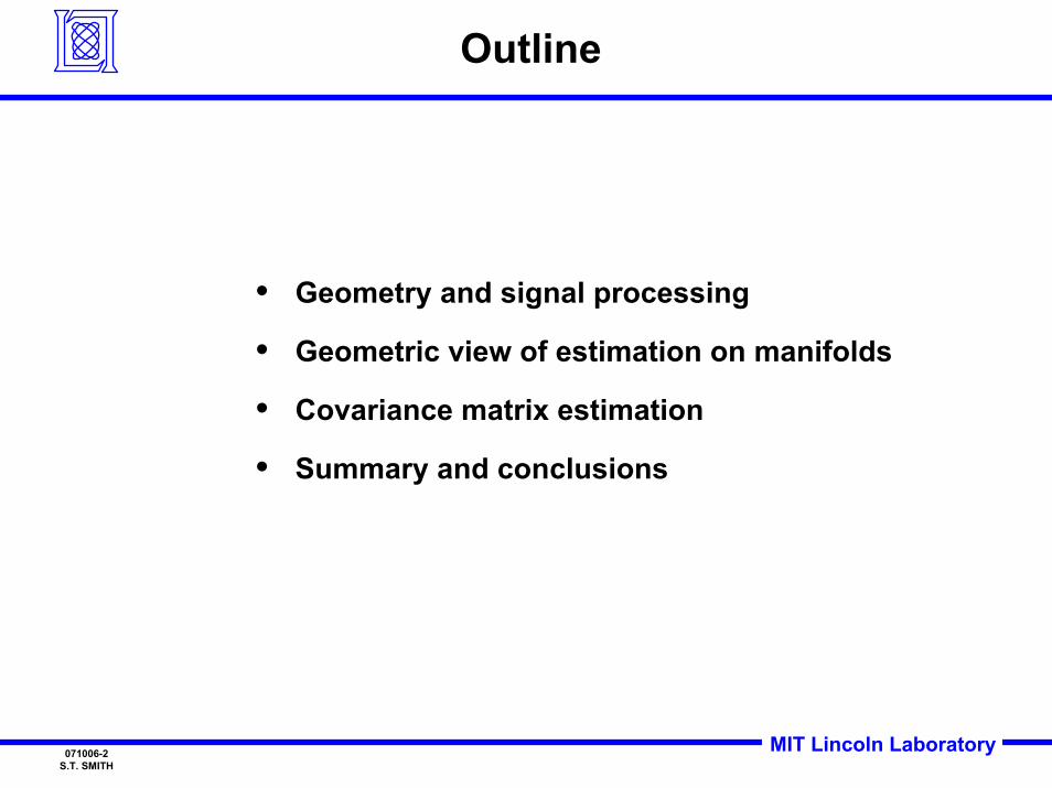
Applications That UseCovariance Matrix Estimation

Air and Ground Surveillance• Space-Time adaptive processing• SAR/GMTI• Tracking

Algorithms and systems analysis for detection, location, and classification of difficult signals all rely onsubspace and covariance-based methods

Algorithms and systems analysis for detection, location, and classification of difficult signals all rely onsubspace and covariance-based methods

Signals Intelligence• Spectral analysis• Superresolution

Robust Navigation• Adaptive beamforming

Undersea Surveillance• Adaptive beamforming• Spectral analysis• Tracking

AdvancedCommunications

• Adaptive beamforming• Spectral analysis• Speech

MIT Lincoln Laboratory071006-4S.T. SMITH

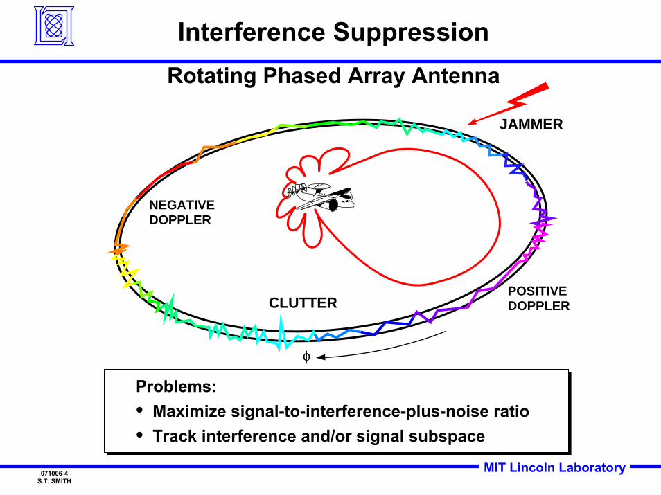
POSITIVEDOPPLER

NEGATIVEDOPPLER

CLUTTER

φ

JAMMER

Interference SuppressionRotating Phased Array Antenna

Problems:• Maximize signal-to-interference-plus-noise ratio• Track interference and/or signal subspace

Problems:• Maximize signal-to-interference-plus-noise ratio• Track interference and/or signal subspace

MIT Lincoln Laboratory071006-5S.T. SMITH

Do

pp

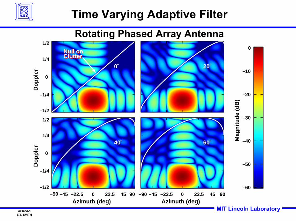
ler 0˚

Null onClutterNull onClutter

–1/2

–1/4

0

1/4

1/2

20˚

Do

pp

ler

Azimuth (deg)

40˚

–90 –45 –22.5 0 22.5 45 90 –1/2

–1/4

0

1/4

1/2

Mag

nit

ud

e (d

B)

–60

–50

–40

–30

–20

–10

0

Azimuth (deg)

60˚

–90 –45 –22.5 0 22.5 45 90

Time Varying Adaptive FilterRotating Phased Array Antenna

MIT Lincoln Laboratory071006-6S.T. SMITH

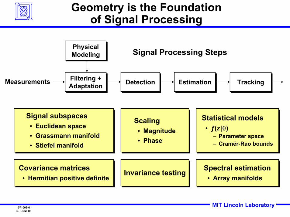
Geometry is the Foundationof Signal Processing

Covariance matrices• Hermitian positive definite

Covariance matrices• Hermitian positive definite

Signal subspaces• Euclidean space• Grassmann manifold • Stiefel manifold

Signal subspaces• Euclidean space• Grassmann manifold • Stiefel manifold

Scaling• Magnitude• Phase

Scaling• Magnitude• Phase

Invariance testingInvariance testing

Statistical models• ƒ(z |θ)

– Parameter space– Cramér-Rao bounds

Statistical models• ƒ(z |θ)

– Parameter space– Cramér-Rao bounds

Spectral estimation• Array manifolds

Spectral estimation• Array manifolds

Filtering +AdaptationFiltering +Adaptation DetectionDetection EstimationEstimation

PhysicalModelingPhysicalModeling

Measurements

Signal Processing Steps

TrackingTracking

MIT Lincoln Laboratory071006-7S.T. SMITH

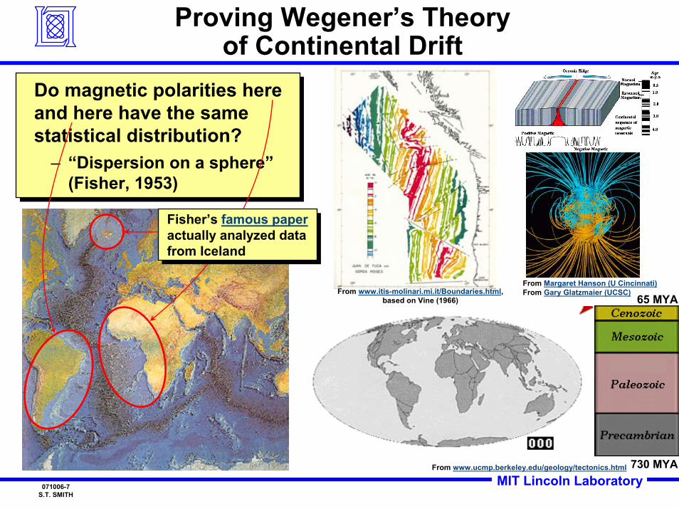
Proving Wegener’s Theoryof Continental Drift

From Margaret Hanson (U Cincinnati)From Gary Glatzmaier (UCSC)

From www.ucmp.berkeley.edu/geology/tectonics.html

From www.itis-molinari.mi.it/Boundaries.html,based on Vine (1966)

Do magnetic polarities here and here have the same statistical distribution?

– “Dispersion on a sphere”(Fisher, 1953)

Do magnetic polarities here and here have the same statistical distribution?

– “Dispersion on a sphere”(Fisher, 1953)

Fisher’s famous paperactually analyzed data from Iceland

Fisher’s famous paperactually analyzed data from Iceland

730 MYA

65 MYA

MIT Lincoln Laboratory071006-8S.T. SMITH

Outline

• Geometry and signal processing

• Geometric view of estimation on manifolds

• Covariance matrix estimation

• Summary and conclusions

MIT Lincoln Laboratory071006-9S.T. SMITH

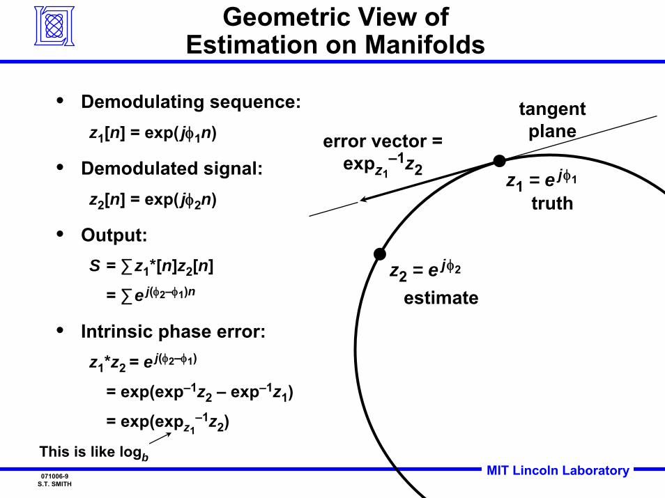
Geometric View ofEstimation on Manifolds

• Demodulating sequence:z1[n] = exp( jφ1n)

• Demodulated signal:z2[n] = exp( jφ2n)

• Output:S = ∑z1*[n]z2[n]

= ∑e j(φ2–φ1)n

• Intrinsic phase error:z1*z2 = e j(φ2–φ1)

= exp(exp–1z2 – exp–1z1)

= exp(expz1–1z2)

This is like logb

z2 = e jφ2

z1 = e jφ1

error vector = expz1

–1z2

tangent plane

truth

estimate

MIT Lincoln Laboratory071006-10S.T. SMITH

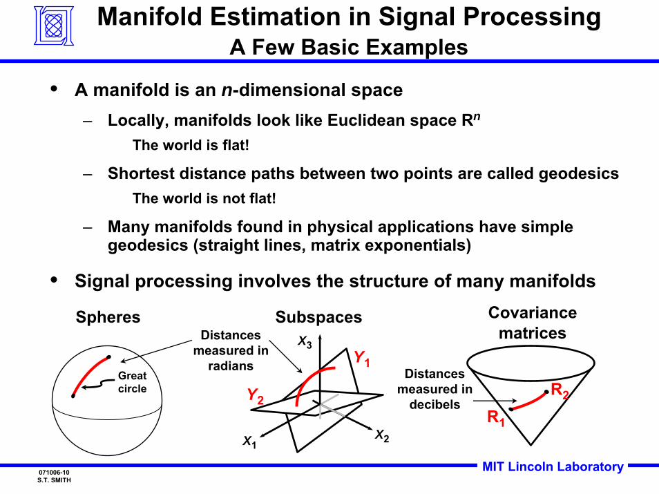
Manifold Estimation in Signal ProcessingA Few Basic Examples

• A manifold is an n-dimensional space– Locally, manifolds look like Euclidean space Rn

The world is flat!

– Shortest distance paths between two points are called geodesics The world is not flat!

– Many manifolds found in physical applications have simple geodesics (straight lines, matrix exponentials)

• Signal processing involves the structure of many manifolds

Spheres

Great circle

Subspaces Covariancematrices

X1X2

X3

R1

R2

Y1

Y2

Distancesmeasured in

radians Distancesmeasured in

decibels

MIT Lincoln Laboratory071006-11S.T. SMITH

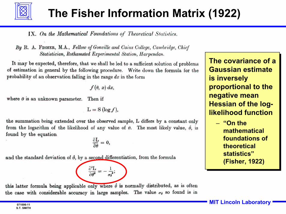
The Fisher Information Matrix (1922)

The covariance of a Gaussian estimate is inversely proportional to the negative mean Hessian of the log-likelihood function

– “On the mathematical foundations of theoretical statistics”(Fisher, 1922)

The covariance of a Gaussian estimate is inversely proportional to the negative mean Hessian of the log-likelihood function

– “On the mathematical foundations of theoretical statistics”(Fisher, 1922)

MIT Lincoln Laboratory071006-12S.T. SMITH

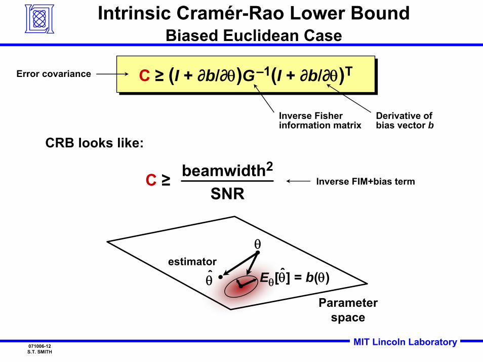
C ≥ (I + ∂b/∂θ)G–1(I + ∂b/∂θ)TC ≥ (I + ∂b/∂θ)G–1(I + ∂b/∂θ)T

Intrinsic Cramér-Rao Lower BoundBiased Euclidean Case

C ≥ beamwidth2

SNRInverse FIM+bias term

Error covariance

Inverse Fisher information matrix

CRB looks like:

Derivative of bias vector b

θ̂

θ

Parameterspace

estimatorˆEθ[θ] = b(θ)

MIT Lincoln Laboratory071006-13S.T. SMITH

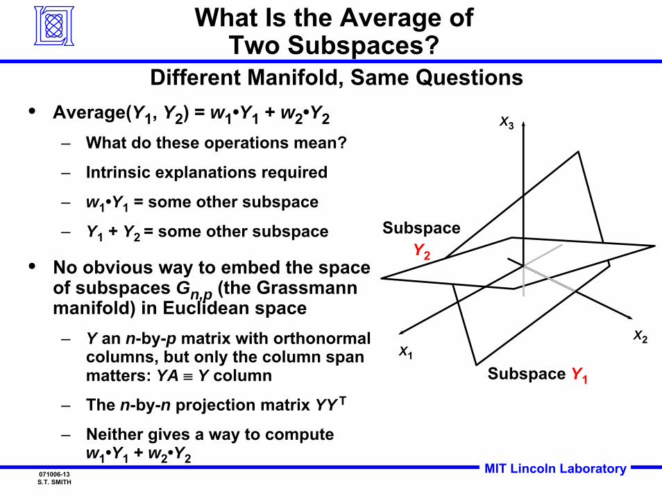
What Is the Average ofTwo Subspaces?

• Average(Y1, Y2) = w1•Y1 + w2•Y2– What do these operations mean?

– Intrinsic explanations required

– w1•Y1 = some other subspace

– Y1 + Y2 = some other subspace

• No obvious way to embed the space of subspaces Gn,p (the Grassmann manifold) in Euclidean space– Y an n-by-p matrix with orthonormal

columns, but only the column span matters: YA ≡ Y column

– The n-by-n projection matrix YY T

– Neither gives a way to compute w1•Y1 + w2•Y2

Different Manifold, Same Questions

X1

X2

X3

Subspace Y1

SubspaceY2

MIT Lincoln Laboratory071006-14S.T. SMITH

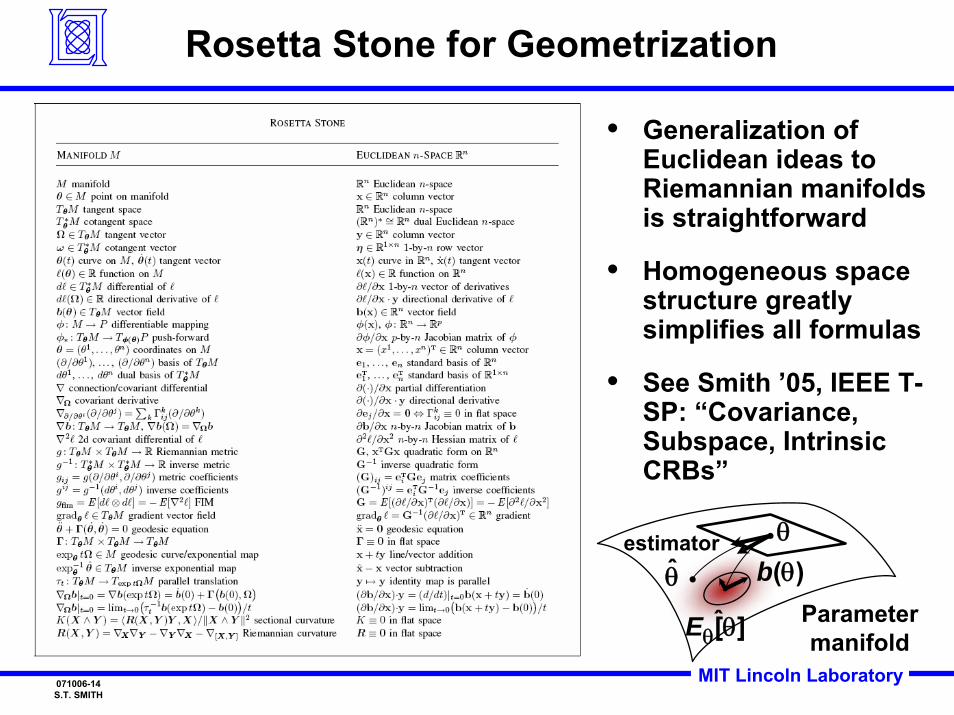
Rosetta Stone for Geometrization

θ

θ̂

ˆEθ[θ] Parametermanifold

estimatorb(θ)

• Generalization of Euclidean ideas to Riemannian manifolds is straightforward

• Homogeneous space structure greatly simplifies all formulas

• See Smith ’05, IEEE T-SP: “Covariance, Subspace, Intrinsic CRBs”

MIT Lincoln Laboratory071006-15S.T. SMITH

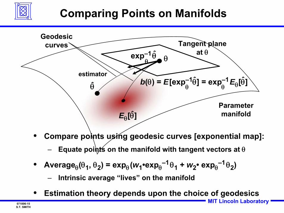
Comparing Points on Manifolds

• Compare points using geodesic curves [exponential map]:– Equate points on the manifold with tangent vectors at θ

• Averageθ(θ1, θ2) = expθ(w1•expθ–1 θ1 + w2• expθ

–1 θ2)– Intrinsic average “lives” on the manifold

• Estimation theory depends upon the choice of geodesics

θ

θ̂

ˆEθ[θ]Parametermanifold

estimator

Tangent planeat θexp–1 θ̂

θ

Geodesiccurves

b(θ) = E[exp–1θ] = exp–1Eθ[θ]ˆθ

ˆθ

MIT Lincoln Laboratory071006-16S.T. SMITH

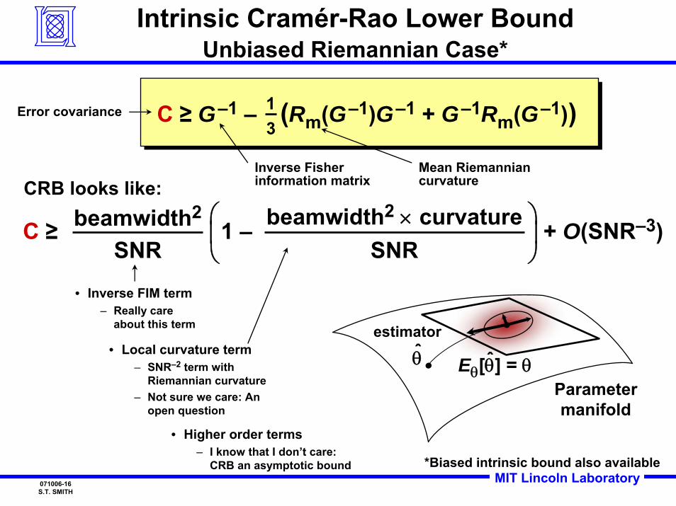
Intrinsic Cramér-Rao Lower BoundUnbiased Riemannian Case*

θ̂ ˆEθ[θ] = θParametermanifold

estimator

C ≥ beamwidth2

SNR⎛⎜⎝

⎞⎟⎠

1 – beamwidth2 × curvatureSNR

+ O(SNR–3)

• Inverse FIM term– Really care

about this term

• Local curvature term– SNR–2 term with

Riemannian curvature– Not sure we care: An

open question

• Higher order terms– I know that I don’t care:

CRB an asymptotic bound

C ≥ G–1 – (Rm(G–1)G–1 + G–1Rm(G–1))C ≥ G–1 – (Rm(G–1)G–1 + G–1Rm(G–1))

Inverse Fisher information matrix

Mean Riemannian curvature

13

CRB looks like:

Error covariance

*Biased intrinsic bound also available

MIT Lincoln Laboratory071006-17S.T. SMITH

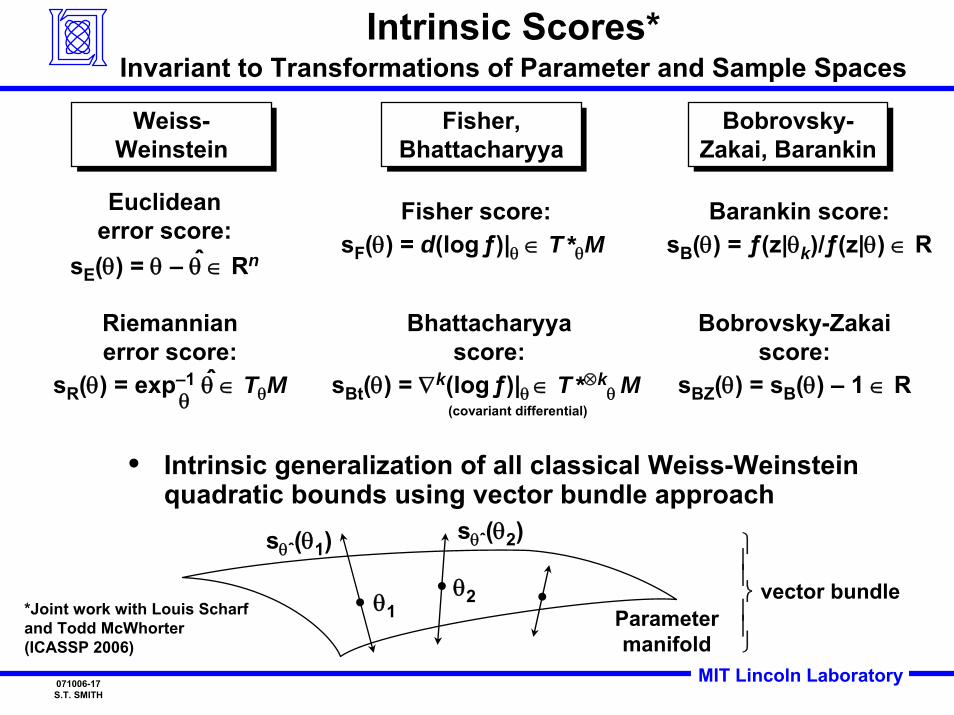
Intrinsic Scores*Invariant to Transformations of Parameter and Sample Spaces

Weiss-WeinsteinWeiss-

WeinsteinFisher,

BhattacharyyaFisher,

BhattacharyyaBobrovsky-

Zakai, BarankinBobrovsky-

Zakai, Barankin

Fisher score:sF(θ) = d(log ƒ)|θ ∈ T*θM

Riemannianerror score:

sR(θ) = exp–1 θ ∈ TθMˆθ

Euclideanerror score:

sE(θ) = θ – θ ∈ Rnˆ

Bhattacharyyascore:

sBt(θ) = ∇k(logƒ)|θ ∈ T*⊗kθ M

Bobrovsky-Zakaiscore:

sBZ(θ) = sB(θ) – 1 ∈ R

Barankin score:sB(θ) = ƒ(z|θk)/ƒ(z|θ) ∈ R

• Intrinsic generalization of all classical Weiss-Weinstein quadratic bounds using vector bundle approach

(covariant differential)

Parametermanifold

vector bundle

sθˆ(θ1) ⎫⎪⎬

⎪⎭

⎪

⎪

sθˆ(θ2)

θ1θ2

*Joint work with Louis Scharfand Todd McWhorter (ICASSP 2006)

MIT Lincoln Laboratory071006-18S.T. SMITH

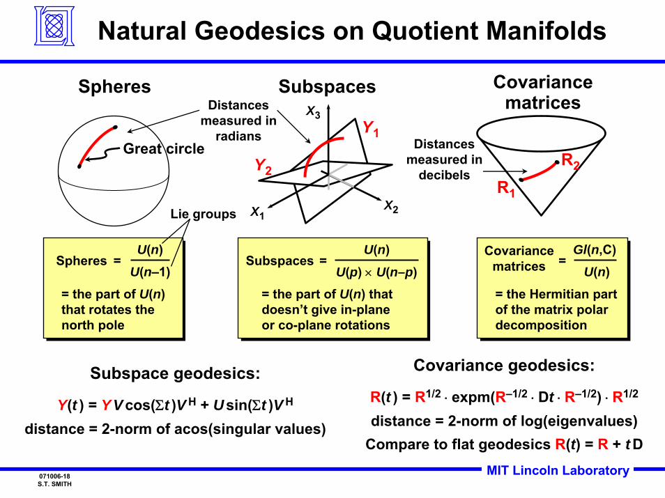
Natural Geodesics on Quotient Manifolds

Spheres

Great circle

Covariance geodesics:

R(t ) = R1/2 ⋅ expm(R–1/2 ⋅ Dt ⋅ R–1/2) ⋅ R1/2

distance = 2-norm of log(eigenvalues)Compare to flat geodesics R(t) = R + t D

Subspace geodesics:

Y(t ) = YVcos(Σt )V H + Usin(Σt )V H

distance = 2-norm of acos(singular values)

Subspaces Covariancematrices

X1X2

X3

Subspaces =U(n)

U(p) × U(n–p) = the part of U(n) that doesn’t give in-plane or co-plane rotations

Covariancematrices =

Gl(n,C)U(n)

= the Hermitian part of the matrix polar decomposition

Spheres =U(n)

U(n–1)= the part of U(n) that rotates the north pole

Lie groups

R1

R2

Y1

Y2

Distancesmeasured in

radians Distancesmeasured in

decibels

MIT Lincoln Laboratory071006-19S.T. SMITH

Outline

• Geometry and signal processing

• Geometric view of estimation on manifolds

• Covariance matrix estimation

• Summary and conclusions

MIT Lincoln Laboratory071006-20S.T. SMITH

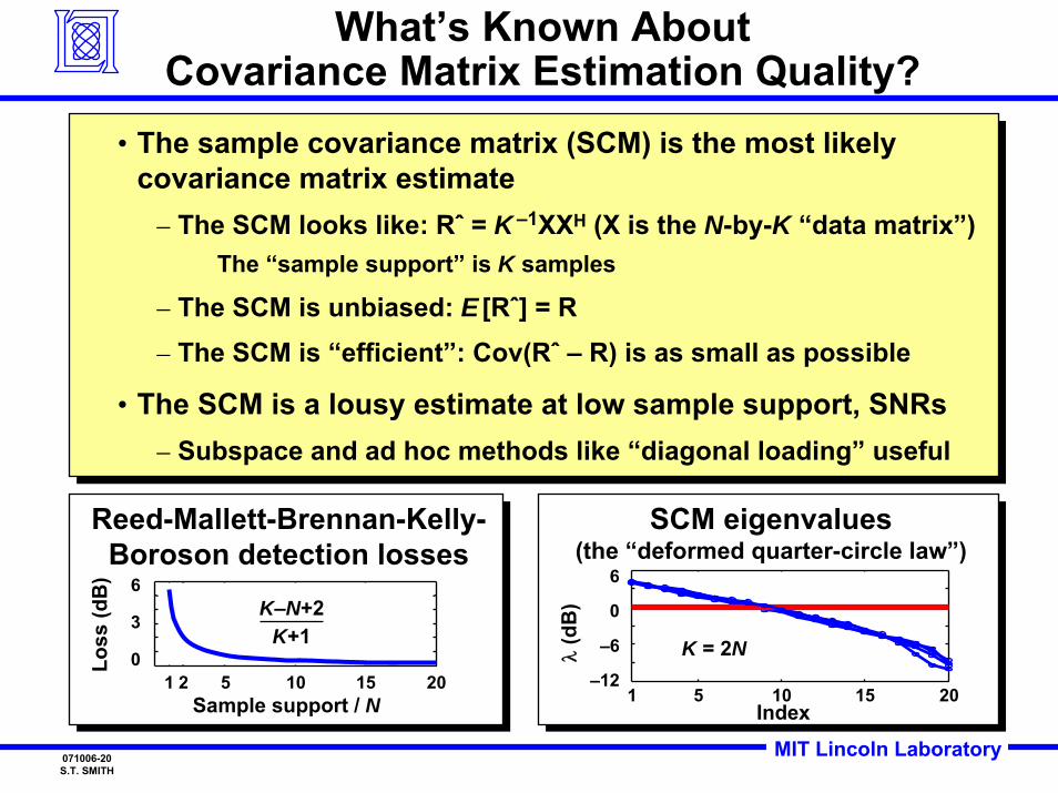
Reed-Mallett-Brennan-Kelly-Boroson detection losses

Reed-Mallett-Brennan-Kelly-Boroson detection losses

1 2 5 10 15 200

3

6

Sample support / N

Loss

(dB

)

K–N+2K+1

SCM eigenvalues(the “deformed quarter-circle law”)

SCM eigenvalues(the “deformed quarter-circle law”)

1 5 10 15 20–12

–6

0

6

Index

λ(d

B)

K = 2N

What’s Known AboutCovariance Matrix Estimation Quality?

• The sample covariance matrix (SCM) is the most likely covariance matrix estimate

– The SCM looks like: Rˆ = K –1XXH (X is the N-by-K “data matrix”)The “sample support” is K samples

– The SCM is unbiased: E [Rˆ] = R– The SCM is “efficient”: Cov(Rˆ – R) is as small as possible

• The SCM is a lousy estimate at low sample support, SNRs– Subspace and ad hoc methods like “diagonal loading” useful

• The sample covariance matrix (SCM) is the most likely covariance matrix estimate

– The SCM looks like: Rˆ = K –1XXH (X is the N-by-K “data matrix”)The “sample support” is K samples

– The SCM is unbiased: E [Rˆ] = R– The SCM is “efficient”: Cov(Rˆ – R) is as small as possible

• The SCM is a lousy estimate at low sample support, SNRs– Subspace and ad hoc methods like “diagonal loading” useful

MIT Lincoln Laboratory071006-21S.T. SMITH

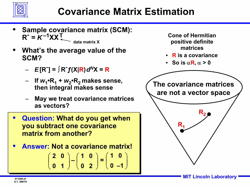
Covariance Matrix Estimation

• Sample covariance matrix (SCM): Rˆ = K–1XXT

• What’s the average value of the SCM?– E [Rˆ] = ∫ Rˆƒ(X|R)dNX = R

– If w1•R1 + w2•R2 makes sense, then integral makes sense

– May we treat covariance matrices as vectors?

• Question: What do you get when you subtract one covariance matrix from another?

• Answer: Not a covariance matrix!20

⎛

⎝⎜⎜

01

⎞⎟⎠⎟

10

⎛

⎝⎜⎜

02

⎞⎟⎠⎟

10

⎛

⎝⎜⎜

0–1

⎞⎟⎠⎟– =

Cone of Hermitian positive definite

matrices• R is a covariance• So is αR, α > 0

R1

R2

The covariance matrices are not a vector space

data matrix X

MIT Lincoln Laboratory071006-22S.T. SMITH

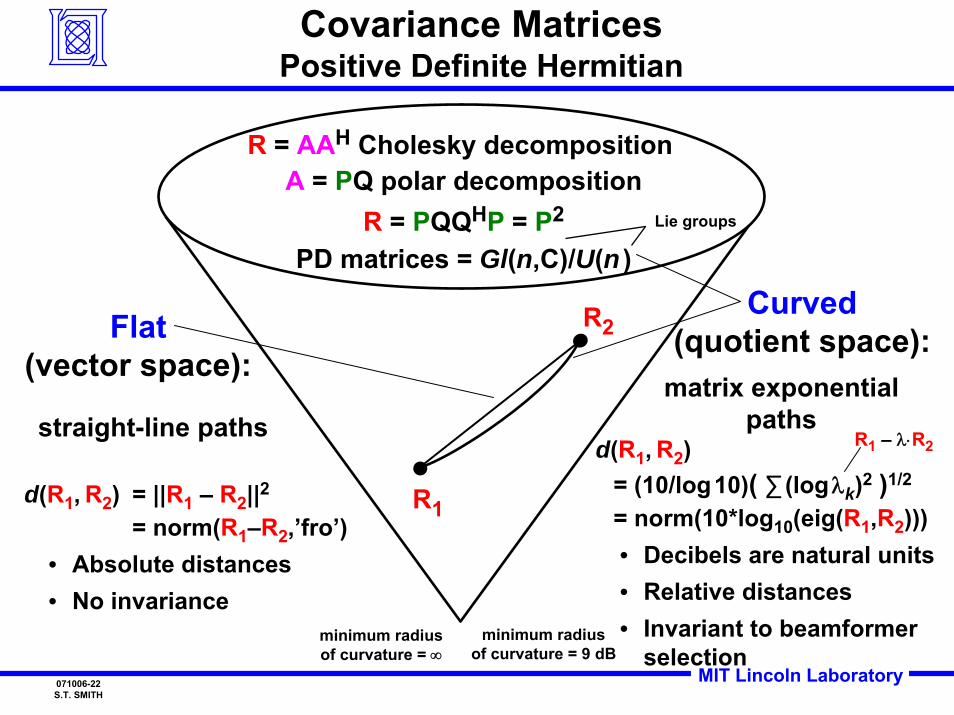
Covariance MatricesPositive Definite Hermitian

R = AAH Cholesky decomposition A = PQ polar decomposition

R = PQQHP = P2

PD matrices = Gl(n,C)/U(n )

Flat(vector space):

Curved(quotient space):

R1

R2

d(R1, R2) = ||R1 – R2||2= norm(R1–R2,’fro’)

• Absolute distances• No invariance

straight-line pathsmatrix exponential

pathsd(R1, R2)

= (10/log10)( ∑ (logλk)2 )1/2

= norm(10*log10(eig(R1,R2)))• Decibels are natural units• Relative distances• Invariant to beamformer

selection

R1 – λ⋅R2

minimum radiusof curvature = ∞

minimum radiusof curvature = 9 dB

Lie groups

MIT Lincoln Laboratory071006-23S.T. SMITH

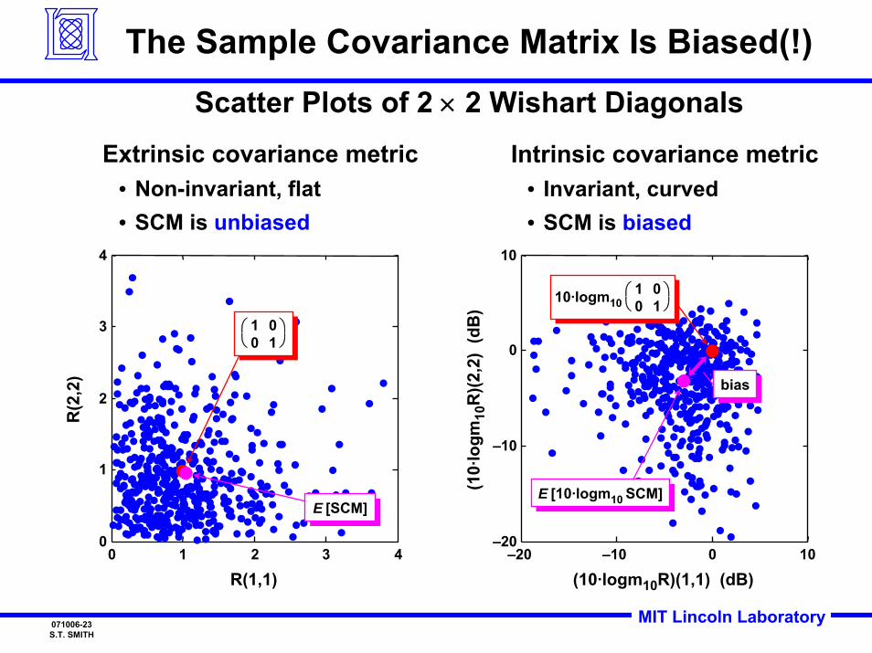
The Sample Covariance Matrix Is Biased(!)

Scatter Plots of 2 × 2 Wishart Diagonals

0 1 2 3 40

1

2

3

4

R(1,1)

R(2

,2)

–20 –10 0 10–20

–10

0

10

(10·logm10R)(1,1) (dB)

(10·

logm

10R

)(2,2

) (d

B)

10

01

⎛⎝

⎞⎠

E [SCM]E [SCM]

10

01

⎛⎝

⎞⎠10·logm10

E [10·logm10 SCM]E [10·logm10 SCM]

Extrinsic covariance metric• Non-invariant, flat• SCM is unbiased

Intrinsic covariance metric• Invariant, curved• SCM is biased

biasbias

MIT Lincoln Laboratory071006-24S.T. SMITH

Covariance matrices flat:

Covariance matrices

R1R2

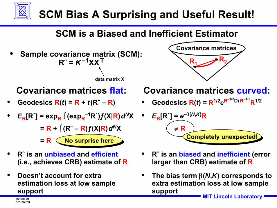
SCM Bias A Surprising and Useful Result!SCM is a Biased and Inefficient Estimator

• Sample covariance matrix (SCM): Rˆ = K–1XX T

data matrix X

• Geodesics R(t) = R + t (Rˆ – R)

• ER[Rˆ] = expR ∫ (expR–1Rˆ)ƒ(X|R)dNX

= R + ∫ (Rˆ – R)ƒ(X|R)dNX

= R

• Rˆ is an unbiased and efficient(i.e., achieves CRB) estimate of R

• Doesn’t account for extra estimation loss at low sample support

No surprise here

• Geodesics R(t) = R1/2eR–1/2DtR–1/2R1/2

• ER[Rˆ] = e–β(N,K)R

≠ R

• Rˆ is an biased and inefficient (error larger than CRB) estimate of R

• The bias term β(N,K) corresponds to extra estimation loss at low sample support

Covariance matrices curved:

No surprise here Completely unexpected!Completely unexpected!

MIT Lincoln Laboratory071006-25S.T. SMITH

1 10

10

Sample support/N

Cov

aria

nce

RM

SE (d

B)

2 5

20

5

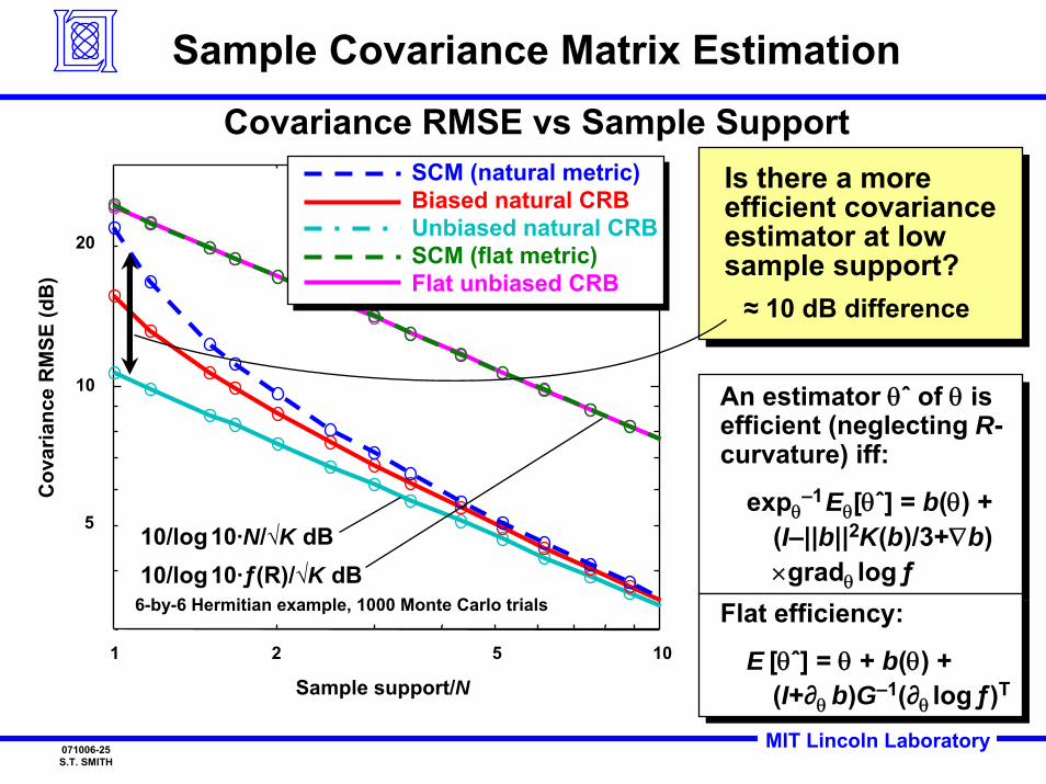
Sample Covariance Matrix EstimationCovariance RMSE vs Sample Support

An estimator θˆ of θ is efficient (neglecting R-curvature) iff:

expθ–1Eθ[θˆ] = b(θ) +

(I–||b||2K(b)/3+∇b) ×gradθ logƒ

An estimator θˆ of θ is efficient (neglecting R-curvature) iff:

expθ–1Eθ[θˆ] = b(θ) +

(I–||b||2K(b)/3+∇b) ×gradθ logƒ

Is there a more efficient covariance estimator at low sample support?≈ 10 dB difference

Is there a more efficient covariance estimator at low sample support?≈ 10 dB difference

SCM (natural metric)Biased natural CRBUnbiased natural CRBSCM (flat metric)Flat unbiased CRB

6-by-6 Hermitian example, 1000 Monte Carlo trials

10/log10·N/√K dB10/log10·ƒ(R)/√K dB

Flat efficiency:

E [θˆ] = θ + b(θ) + (I+∂θ b)G–1(∂θ logƒ)T

Flat efficiency:

E [θˆ] = θ + b(θ) + (I+∂θ b)G–1(∂θ logƒ)T

MIT Lincoln Laboratory071006-26S.T. SMITH

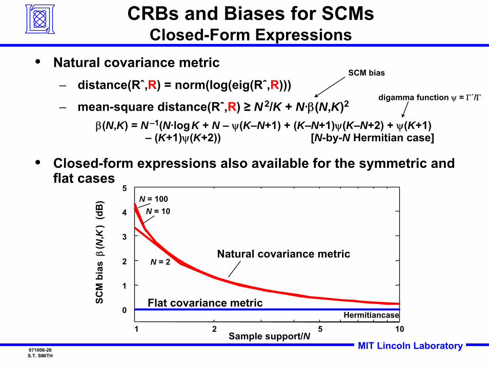
CRBs and Biases for SCMsClosed-Form Expressions

• Natural covariance metric– distance(Rˆ,R) = norm(log(eig(Rˆ,R)))

– mean-square distance(Rˆ,R) ≥ N 2/K + N·β(N,K)2

β(N,K) = N –1(N·logK + N – ψ(K–N+1) + (K–N+1)ψ(K–N+2) + ψ(K+1) – (K+1)ψ(K+2)) [N-by-N Hermitian case]

• Closed-form expressions also available for the symmetric and flat cases

digamma function ψ = Γ´/Γ

SCM bias

0

1

2

3

4

5

SCM

bia

s β

(N,K

) (d

B)

1 10Sample support/N

2 5Hermitiancase

Natural covariance metric

Flat covariance metric

N = 2

N = 100N = 10

MIT Lincoln Laboratory071006-27S.T. SMITH

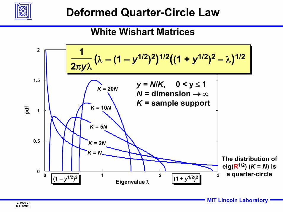
Deformed Quarter-Circle LawWhite Wishart Matrices

The distribution of eig(R1/2) (K = N) is

a quarter-circle0 1 2 30

0.5

1

1.5

2

Eigenvalue λ

pdf

12πyλ

(λ – (1 – y1/2)2)1/2((1 + y1/2)2 – λ)1/2

K = NK = 2N

K = 5N

K = 10N

K = 20N

(1 – y1/2)2(1 – y1/2)2 (1 + y1/2)2(1 + y1/2)2

y = N/K, 0 < y ≤ 1N = dimension → ∞K = sample support

MIT Lincoln Laboratory071006-28S.T. SMITH

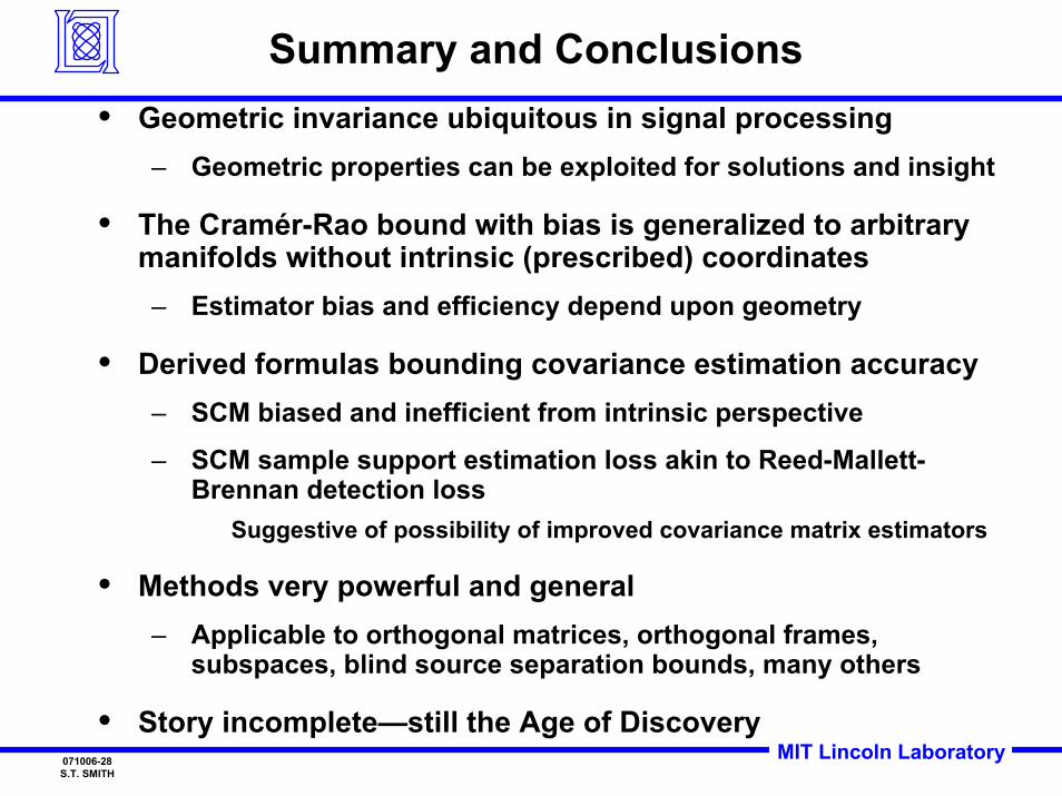
Summary and Conclusions• Geometric invariance ubiquitous in signal processing

– Geometric properties can be exploited for solutions and insight

• The Cramér-Rao bound with bias is generalized to arbitrary manifolds without intrinsic (prescribed) coordinates– Estimator bias and efficiency depend upon geometry

• Derived formulas bounding covariance estimation accuracy– SCM biased and inefficient from intrinsic perspective

– SCM sample support estimation loss akin to Reed-Mallett-Brennan detection loss

Suggestive of possibility of improved covariance matrix estimators

• Methods very powerful and general– Applicable to orthogonal matrices, orthogonal frames,

subspaces, blind source separation bounds, many others

• Story incomplete—still the Age of Discovery