Embed Size (px)
Citation preview

o
Intra-Picture Coding
Intra-Picture Coding
Thomas Wiegand Digital Image Communication 1 / 48
o
Intra-Picture Coding
Outline
Introduction
Transform Coding of Sample Blocks
OverviewOrthogonal Block TransformsScalar QuantizationEntropy Coding
Intra-Picture Prediction
Prediction in Transform DomainSpatial PredictionExperimental Analysis
Block Sizes for Prediction and Transform Coding
Block Size Selection in Video Coding StandardsExperimental Analysis
Summary
Thomas Wiegand Digital Image Communication 2 / 48
o
Intra-Picture Coding Introduction
Intra-Picture Coding
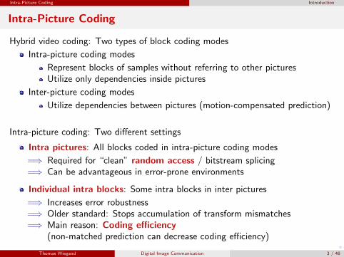
Hybrid video coding: Two types of block coding modes
Intra-picture coding modes
Represent blocks of samples without referring to other picturesUtilize only dependencies inside pictures
Inter-picture coding modes
Utilize dependencies between pictures (motion-compensated prediction)
Intra-picture coding: Two different settings
Intra pictures: All blocks coded in intra-picture coding modes
=⇒ Required for “clean” random access / bitstream splicing=⇒ Can be advantageous in error-prone environments
Individual intra blocks: Some intra blocks in inter pictures
=⇒ Increases error robustness=⇒ Older standard: Stops accumulation of transform mismatches=⇒ Main reason: Coding efficiency
(non-matched prediction can decrease coding efficiency)
Thomas Wiegand Digital Image Communication 3 / 48
o
Intra-Picture Coding Introduction
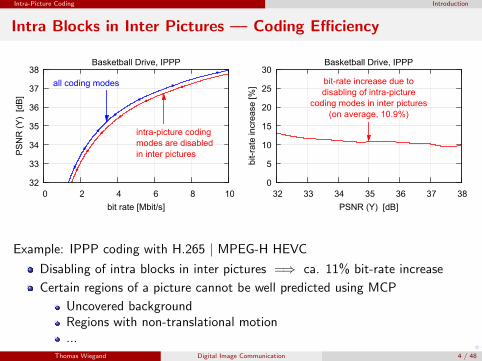
Intra Blocks in Inter Pictures — Coding Efficiency
32
33
34
35
36
37
38
0 2 4 6 8 10
PS
NR
(Y
) [d
B]
bit rate [Mbit/s]
Basketball Drive, IPPP
all coding modes
intra-picture codingmodes are disabledin inter pictures
0
5
10
15
20
25
30
32 33 34 35 36 37 38
bit-
rate
incr
ease
[%]
PSNR (Y) [dB]
Basketball Drive, IPPP
bit-rate increase due todisabling of intra-picture
coding modes in inter pictures(on average, 10.9%)
Example: IPPP coding with H.265 | MPEG-H HEVC
Disabling of intra blocks in inter pictures =⇒ ca. 11% bit-rate increase
Certain regions of a picture cannot be well predicted using MCP
Uncovered backgroundRegions with non-translational motion...
Thomas Wiegand Digital Image Communication 4 / 48
o
Intra-Picture Coding Transform Coding of Sample Blocks
Transform Coding of Sample Blocks
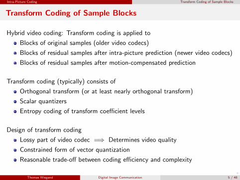
Hybrid video coding: Transform coding is applied to
Blocks of original samples (older video codecs)
Blocks of residual samples after intra-picture prediction (newer video codecs)
Blocks of residual samples after motion-compensated prediction
Transform coding (typically) consists of
Orthogonal transform (or at least nearly orthogonal transform)
Scalar quantizers
Entropy coding of transform coefficient levels
Design of transform coding
Lossy part of video codec =⇒ Determines video quality
Constrained form of vector quantization
Reasonable trade-off between coding efficiency and complexity
Thomas Wiegand Digital Image Communication 5 / 48

o
Intra-Picture Coding Transform Coding of Sample Blocks
Basic Concept of Transform Coding
2D linear
analysis
transform
𝑨
entropy
coding
𝛾
N×M block
of original
samples 𝒔 codewords
𝛼0
𝛼1
𝛼𝑁𝑀−1
𝑡0
𝑡1
𝑡𝑁𝑀−1
𝑞0
𝑞1
𝑞𝑁𝑀−1
scalar quantization
entropy
decoding
𝛾−1
2D linear
synthesis
transform
𝑩
N×M block
of reconstr.
samples 𝒔′codewords
𝛽0
𝛽1
𝛽𝑁𝑀−1
𝑡0′
𝑡1′
𝑞0
𝑞1
𝑞𝑁𝑀−1
scalar decoder mapping
𝑡𝑁𝑀−1′
Thomas Wiegand Digital Image Communication 6 / 48
o
Intra-Picture Coding Orthogonal Block Transform
Orthogonal Block Transform
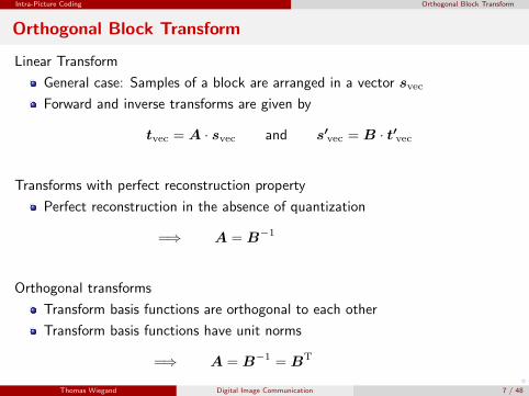
Linear Transform
General case: Samples of a block are arranged in a vector svec
Forward and inverse transforms are given by
tvec = A · svec and s′vec = B · t′vec
Transforms with perfect reconstruction property
Perfect reconstruction in the absence of quantization
=⇒ A = B−1
Orthogonal transforms
Transform basis functions are orthogonal to each other
Transform basis functions have unit norms
=⇒ A = B−1 = BT
Thomas Wiegand Digital Image Communication 7 / 48
o
Intra-Picture Coding Orthogonal Block Transform
Orthogonal Block Transform
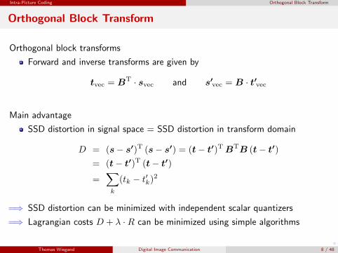
Orthogonal block transforms
Forward and inverse transforms are given by
tvec = BT · svec and s′vec = B · t′vec
Main advantage
SSD distortion in signal space = SSD distortion in transform domain
D = (s− s′)T (s− s′) = (t− t′)T BTB (t− t′)
= (t− t′)T (t− t′)
=∑k
(tk − t′k)2
=⇒ SSD distortion can be minimized with independent scalar quantizers
=⇒ Lagrangian costs D + λ ·R can be minimized using simple algorithms
Thomas Wiegand Digital Image Communication 8 / 48

o
Intra-Picture Coding Orthogonal Block Transform
Separable Block Transforms
Separable Transforms
N×M blocks of samples and transform coefficients
Forward and inverse transforms are given by
t = BTV · s ·BH and s′ = BV · t′ ·BT
H
Interpretation (forward transform)1 Transform all columns of the block using the vertical transform2 Transform all rows of the intermediate block using the horizontal transform
or1 Transform all rows of the block using the horizontal transform2 Transform all columns of the intermediate block using the vertical transform
Advantage of separable transforms
Significantly reduced complexity
Potential loss in coding efficiency is very small (due to 2D character of data)
Thomas Wiegand Digital Image Communication 9 / 48

o
Intra-Picture Coding Orthogonal Block Transform
2D Discrete Cosine Transform (DCT) of Type II
2D Discrete Cosine Transform of type II (DCT-II)
Horizontal and vertical transforms BH and BV are DCTs of type II
Optimal transform for Gauss-Markov sources with %→ 1
N×N inverse transform matrix BDCT = {bik} is given by coefficients
bik =ak√N
cos
(π
Nk
(i+
1
2
))with ak =
{1 : i = 0√
2 : i > 0
Integer Transforms
Disadvantage of DCT: Most matrix coefficients are irrational numbers
=⇒ Have to be approximated by binary numbers with finite precision=⇒ Mismatches if encoder and decoder use different approximations
New video coding standards specify integer approximation of DCT
=⇒ Same approximation is used in all implementations=⇒ No encoder/decoder mismatches due to different implementations
Thomas Wiegand Digital Image Communication 10 / 48

o
Intra-Picture Coding Orthogonal Block Transform
2D DCT Example — Step 1: Vertical Transform
Example for a 16×16 DCT
Step 1: Column-wise DCT on image block yielding intermediate block oftransform coefficients
Notice the energy concentration in the first row (DC coefficients)
Thomas Wiegand Digital Image Communication 11 / 48

o
Intra-Picture Coding Orthogonal Block Transform
2D DCT Example — Step 2: Horizontal Transform
Example for a 16×16 DCT
Step 2: Row-wise DCT on intermediate block of transform coefficientsyielding the final block of DCT coefficients
Notice the energy concentration in the DC coefficient (top-left)
Thomas Wiegand Digital Image Communication 12 / 48
o
Intra-Picture Coding Orthogonal Block Transform
Transform Gain
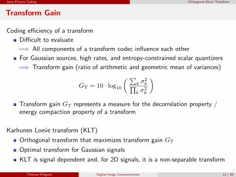
Coding efficiency of a transform
Difficult to evaluate
=⇒ All components of a transform codec influence each other
For Gaussian sources, high rates, and entropy-constrained scalar quantizers
=⇒ Transform gain (ratio of arithmetic and geometric mean of variances)
GT = 10 · log10
( ∑k σ
2k∏
k σ2k
)Transform gain GT represents a measure for the decorrelation property /energy compaction property of a transform
Karhunen Loeve transform (KLT)
Orthogonal transform that maximizes transform gain GT
Optimal transform for Gaussian signals
KLT is signal dependent and, for 2D signals, it is a non-separable transform
Thomas Wiegand Digital Image Communication 13 / 48
o
Intra-Picture Coding Orthogonal Block Transform
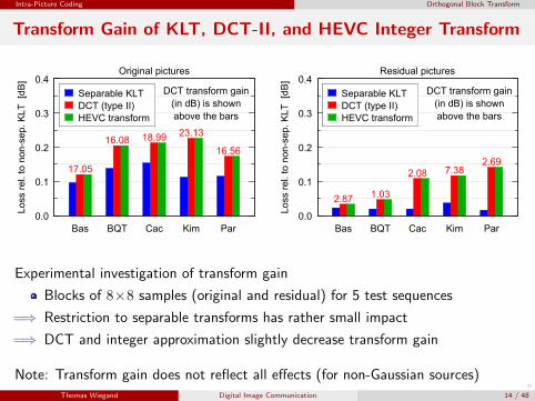
Transform Gain of KLT, DCT-II, and HEVC Integer Transform
0.0
0.1
0.2
0.3
0.4
Bas BQT Cac Kim Par
Loss
rel
. to
non-
sep.
KLT
[dB
]
Original pictures
17.05
16.08 18.99 23.13
16.56
Separable KLTDCT (type II)HEVC transform
DCT transform gain(in dB) is shownabove the bars
0.0
0.1
0.2
0.3
0.4
Bas BQT Cac Kim Par
Loss
rel
. to
non-
sep.
KLT
[dB
]
Residual pictures
2.87 1.03
2.08 7.382.69
Separable KLTDCT (type II)HEVC transform
DCT transform gain(in dB) is shownabove the bars
Experimental investigation of transform gain
Blocks of 8×8 samples (original and residual) for 5 test sequences
=⇒ Restriction to separable transforms has rather small impact
=⇒ DCT and integer approximation slightly decrease transform gain
Note: Transform gain does not reflect all effects (for non-Gaussian sources)Thomas Wiegand Digital Image Communication 14 / 48
o
Intra-Picture Coding Orthogonal Block Transform
Optimal Orthogonal Transform at High Rates
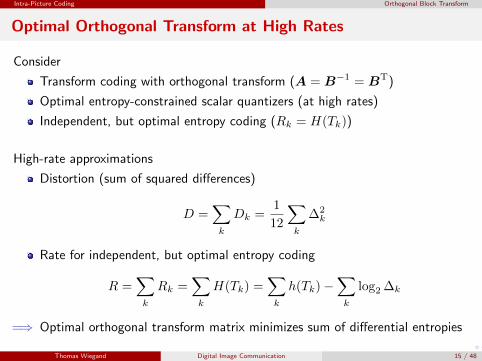
Consider
Transform coding with orthogonal transform (A = B−1 = BT)
Optimal entropy-constrained scalar quantizers (at high rates)
Independent, but optimal entropy coding (Rk = H(Tk))
High-rate approximations
Distortion (sum of squared differences)
D =∑k
Dk =1
12
∑k
∆2k
Rate for independent, but optimal entropy coding
R =∑k
Rk =∑k
H(Tk) =∑k
h(Tk)−∑k
log2 ∆k
=⇒ Optimal orthogonal transform matrix minimizes sum of differential entropies
Thomas Wiegand Digital Image Communication 15 / 48
o
Intra-Picture Coding Orthogonal Block Transform
Optimal Orthogonal Transform at High Rates
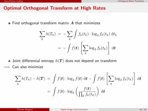
Find orthogonal transform matrix A that minimizes∑k
h(Tk) = −∑k
∫fk(tk) · log2 fk(tk) dtk
= −∫f(t)
[∑k
log2 fk(tk)
]dt
Joint differential entropy h(T ) does not depend on transform
=⇒ Can also minimize
∑k
h(Tk)− h(T ) =
∫f(t) · log2 f(t) dt−
∫f(t)
[∑k
log2 fk(tk)
]dt
=
∫f(t) · log2
(f(t)∏k fk(tk)
)dt
Thomas Wiegand Digital Image Communication 16 / 48
o
Intra-Picture Coding Orthogonal Block Transform
Optimal Orthogonal Transform at High Rates
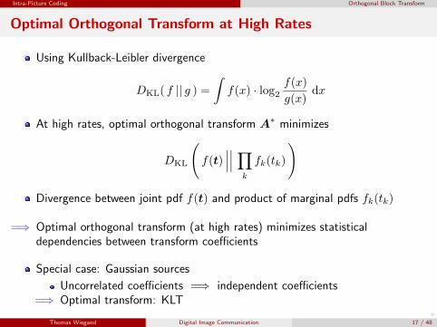
Using Kullback-Leibler divergence
DKL( f || g ) =
∫f(x) · log2
f(x)
g(x)dx
At high rates, optimal orthogonal transform A∗ minimizes
DKL
(f(t)
∣∣∣∣∣∣ ∏k
fk(tk)
)
Divergence between joint pdf f(t) and product of marginal pdfs fk(tk)
=⇒ Optimal orthogonal transform (at high rates) minimizes statisticaldependencies between transform coefficients
Special case: Gaussian sources
Uncorrelated coefficients =⇒ independent coefficients=⇒ Optimal transform: KLT
Thomas Wiegand Digital Image Communication 17 / 48
o
Intra-Picture Coding Orthogonal Block Transform
Coding Optimal Transform (COT)
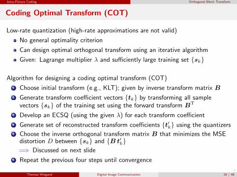
Low-rate quantization (high-rate approximations are not valid)
No general optimality criterion
Can design optimal orthogonal transform using an iterative algorithm
Given: Lagrange multiplier λ and sufficiently large training set {sk}
Algorithm for designing a coding optimal transform (COT)
1 Choose initial transform (e.g., KLT); given by inverse transform matrix B
2 Generate transform coefficient vectors {tk} by transforming all samplevectors {sk} of the training set using the forward transform BT
3 Develop an ECSQ (using the given λ) for each transform coefficient
4 Generate set of reconstructed transform coefficients {t′k} using the quantizers5 Choose the inverse orthogonal transform matrix B that minimizes the MSE
distortion D between {sk} and {B t′k}=⇒ Discussed on next slide
6 Repeat the previous four steps until convergence
Thomas Wiegand Digital Image Communication 18 / 48
o
Intra-Picture Coding Orthogonal Block Transform
Coding Optimal Transform (COT)
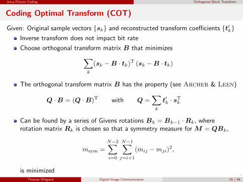
Given: Original sample vectors {sk} and reconstructed transform coefficients {t′k}Inverse transform does not impact bit rate
Choose orthogonal transform matrix B that minimizes∑k
(sk −B · tk)T (sk −B · tk)
The orthogonal transform matrix B has the property (see Archer & Leen)
Q ·B = (Q ·B)T with Q =∑k
t′k · sTk
Can be found by a series of Givens rotations Bk = Bk−1 ·Rk, whererotation matrix Rk is chosen so that a symmetry measure for M = QBk,
msym =
N−2∑i=0
N−1∑j=i+1
(mij −mji)2,
is minimizedThomas Wiegand Digital Image Communication 19 / 48

o
Intra-Picture Coding Orthogonal Block Transform
Coding Efficiency of KLT, DCT, COT
-0.35
-0.30
-0.25
-0.20
-0.15
-0.10
-0.05
0.00
0.05
0 50 100 150 200 250
Loss
rel
. to
non-
sep.
KLT
[dB
]
bit rate (first-order entropy) [Mbit/s]
Cactus (original pictures)
separable KLT
DCT (type II)COT
-0.10
-0.08
-0.06
-0.04
-0.02
0.00
0.02
0.04
0.06
0 50 100 150 200 250
Loss
rel
. to
non-
sep.
KLT
[dB
]
bit rate (first-order entropy) [Mbit/s]
Cactus (residual pictures)
separable KLT
DCT (type II)
COT
Coding experiment for 8×8 blocks of original and residual pictures
Entropy-constrained scalar quantizers & optimal independent entropy coding
Compare non-separable KLT, separable KLT, DCT-II, and COT
=⇒ 2D DCT represents a reasonable choice for transform coding
Signal independent, low complexity, no side informationRather small losses in coding efficiency compared to KLT & COT
Thomas Wiegand Digital Image Communication 20 / 48

o
Intra-Picture Coding Scalar Quantization
Distribution of Transform Coefficients
Distribution of DCT coefficients for typical video pictures / residual blocks
Assume: Samples inside a block are identically distributed
Each DCT coefficient: Weighted sum of samples inside a block
=⇒ Central limit theorem: Coefficients have nearly Gaussian distribution
But: Samples variance σ2S changes across blocks
Coefficient variances σ2i are proportional to samples variance σ2
S
=⇒ Model for transform coefficient distribution
fi(t) =
∞∫0
fi(t|σ2i ) fi(σ
2i ) dσ2
i with fi(t|σ2i ) =
1√2πσ2
i
e− t2
2σ2i
Model for distribution of block variances σ2S
Exponential distribution
Transform coefficient variances are proportional to block variances
fi(σ2i ) = a · e−a σ
2i
Thomas Wiegand Digital Image Communication 21 / 48
o
Intra-Picture Coding Scalar Quantization
Distribution of Transform Coefficients
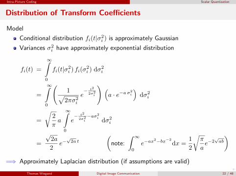
Model
Conditional distribution fi(t|σ2i ) is approximately Gaussian
Variances σ2i have approximately exponential distribution
fi(t) =
∞∫0
fi(t|σ2i ) fi(σ
2i ) dσ2
i
=
∞∫0
(1√
2πσ2i
e− t2
2σ2i
) (a · e−a σ
2i
)dσ2
i
=
√2
πa
∞∫0
e− t2
2σ2i
−aσ2i
dσ2i
=
√2a
2e−√2a t
(note:
∫ ∞0
e−ax2−bx−2
dx =1
2
√π
ae−2√ab
)=⇒ Approximately Laplacian distribution (if assumptions are valid)
Thomas Wiegand Digital Image Communication 22 / 48
o
Intra-Picture Coding Scalar Quantization
Distribution of Transform Coefficients
0.00
0.01
0.02
0.03
0.04
0.05
0.06
0.07
0.08
-30 -20 -10 0 10 20 30
prob
abili
ty d
ensi
ty
transform coefficient value
Transform coefficient t1,1 (residual)
histogram
approximation byLaplacian pdf
(better fit)
approximation byGaussian pdf
0.00
0.05
0.10
0.15
0.20
0.25
0.30
-8 -6 -4 -2 0 2 4 6 8
prob
abili
ty d
ensi
ty
transform coefficient value
Transform coefficient t2,4 (residual)
histogram
approximation byLaplacian pdf
approximation byGaussian pdf(better fit)
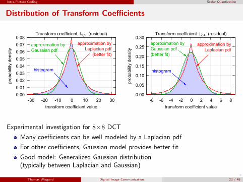
Experimental investigation for 8×8 DCT
Many coefficients can be well modeled by a Laplacian pdf
For other coefficients, Gaussian model provides better fit
Good model: Generalized Gaussian distribution(typically between Laplacian and Gaussian)
Thomas Wiegand Digital Image Communication 23 / 48
o
Intra-Picture Coding Scalar Quantization
Scalar Quantization
Consider
Scalar quantization of transform coefficients
Separate quantization of transform coefficient
Assume independent, but optimal entropy coding
Optimal scalar quantizers
Entropy-constrained scalar quantizers (ECSQ)
ECSQs depend on distribution of transform coefficients
Require transmission of reconstruction levels
=⇒ Not used in practical video codecs
Scalar quantizers used in practice
Uniform reconstruction quantizers (URQs)
URQs with extra-wide dead zone (older video coding standards)
Thomas Wiegand Digital Image Communication 24 / 48

o
Intra-Picture Coding Scalar Quantization
Uniform Reconstruction Quantizers (URQs)
s
s'0 s'1 s'2 s'3 s'4s'-1s'-2s'-3s'-4
0 Δ 1·Δ 3·Δ 4·Δ-Δ-2·Δ-3·Δ-4·Δ
u-3 u-2 u-1 u0 u1 u2 u3 u4
z3 z2 z1 z0 z0 z1 z2 z3
Design of uniform reconstruction quantizers
Equally spaced reconstruction levels (indicated by step size ∆)
Simple decoder mappingt′ = ∆ · q
Encoder has freedom to adapt decision thresholds to source
Decision thresholds can be specified by quantization offsets zk (see figure)
Iterative design algorithm similar to that for ECSQs (not discussed in lecture)
Thomas Wiegand Digital Image Communication 25 / 48
o
Intra-Picture Coding Scalar Quantization
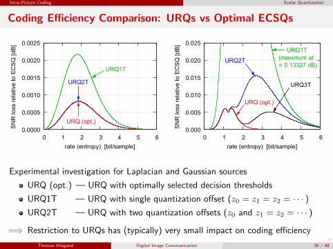
Coding Efficiency Comparison: URQs vs Optimal ECSQs
0.0000
0.0005
0.0010
0.0015
0.0020
0.0025
0 1 2 3 4 5 6
SN
R lo
ss r
elat
ive
to E
CS
Q [d
B]
rate (entropy) [bit/sample]
URQ (opt.)
URQ2T
URQ1T
0.000
0.005
0.010
0.015
0.020
0.025
0 1 2 3 4 5 6
SN
R lo
ss r
elat
ive
to E
CS
Q [d
B]
rate (entropy) [bit/sample]
URQ (opt.)
URQ3T
URQ2T
URQ1T(maximum at
≈ 0.13327 dB)
Experimental investigation for Laplacian and Gaussian sources
URQ (opt.) — URQ with optimally selected decision thresholds
URQ1T — URQ with single quantization offset (z0 = z1 = z2 = · · · )URQ2T — URQ with two quantization offsets (z0 and z1 = z2 = · · · )
=⇒ Restriction to URQs has (typically) very small impact on coding efficiency
Thomas Wiegand Digital Image Communication 26 / 48

o
Intra-Picture Coding Scalar Quantization
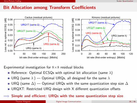
Bit Allocation among Transform Coefficients
Optimal bit allocation
=⇒ All scalar quantizers are designed using the same Lagrange multiplier λ
High-rate approximation for URQs
Operational distortion-rate function Dk(Rk) for component quantizers
Dk(Rk) = ε2k · σ2k · 2−2Rk
Optimal bit allocation
λ = −dDk
dRk= 2 ln 2 · ε2k · σ2
k · 2−2Rk = 2 ln 2 ·Dk = const
High-rate approximation for distortion
Dk =1
12·∆2
k
=⇒ High-rate bit allocation rule
∆k = const
Thomas Wiegand Digital Image Communication 27 / 48
o
Intra-Picture Coding Scalar Quantization
Bit Allocation among Transform Coefficients
0.00
0.01
0.02
0.03
0.04
0.05
0.06
0 50 100 150 200 250
Loss
rel
. to
optim
al E
CS
Q [
dB]
bit rate (first-order entropy) [Mbit/s]
Cactus (residual pictures)
URQ (same λ)
URQ (same Δ)
URQ2T (same Δ)
URQ1T (same Δ)
0.00
0.01
0.02
0.03
0.04
0.05
0.06
0 20 40 60 80 100 120
Loss
rel
. to
optim
al E
CS
Q [
dB]
bit rate (first-order entropy) [Mbit/s]
Kimono (residual pictures)
URQ (same λ)URQ (same Δ)
URQ2T (same Δ)
URQ1T (same Δ)
Experimental investigation for 8×8 residual blocks
Reference: Optimal ECSQs with optimal bit allocation (same λ)
URQ (same λ ) — Optimal URQs, all designed for the same λ
URQ (same ∆) — Optimal URQs with the same quantization step size ∆
URQXT: Restricted URQ design with X different quantization offsets
=⇒ Simple and efficient: URQs with the same quantization step size
Thomas Wiegand Digital Image Communication 28 / 48
o
Intra-Picture Coding Entropy Coding of Transform Coefficient Levels
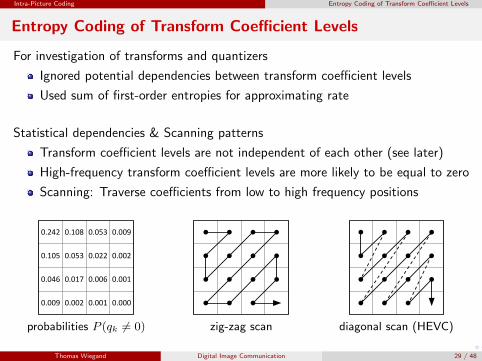
Entropy Coding of Transform Coefficient Levels
For investigation of transforms and quantizers
Ignored potential dependencies between transform coefficient levels
Used sum of first-order entropies for approximating rate
Statistical dependencies & Scanning patterns
Transform coefficient levels are not independent of each other (see later)
High-frequency transform coefficient levels are more likely to be equal to zero
Scanning: Traverse coefficients from low to high frequency positions
0.242 0.108 0.053 0.009
0.105 0.053 0.022 0.002
0.046 0.017 0.006 0.001
0.009 0.002 0.001 0.000
probabilities P (qk 6= 0) zig-zag scan diagonal scan (HEVC)
Thomas Wiegand Digital Image Communication 29 / 48
o
Intra-Picture Coding Entropy Coding of Transform Coefficient Levels
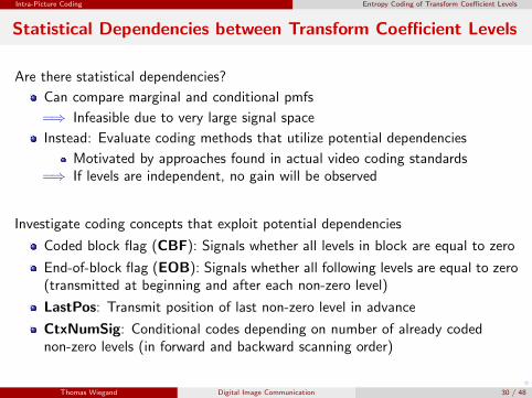
Statistical Dependencies between Transform Coefficient Levels
Are there statistical dependencies?
Can compare marginal and conditional pmfs
=⇒ Infeasible due to very large signal space
Instead: Evaluate coding methods that utilize potential dependencies
Motivated by approaches found in actual video coding standards=⇒ If levels are independent, no gain will be observed
Investigate coding concepts that exploit potential dependencies
Coded block flag (CBF): Signals whether all levels in block are equal to zero
End-of-block flag (EOB): Signals whether all following levels are equal to zero(transmitted at beginning and after each non-zero level)
LastPos: Transmit position of last non-zero level in advance
CtxNumSig: Conditional codes depending on number of already codednon-zero levels (in forward and backward scanning order)
Thomas Wiegand Digital Image Communication 30 / 48

o
Intra-Picture Coding Entropy Coding of Transform Coefficient Levels
Statistical Dependencies between Transform Coefficient Levels
-14
-12
-10
-8
-6
-4
-2
0
0 10 20 30 40 50 60 70 80
bit-
rate
incr
ease
[%]
bit rate (first-order entropy) [Mbit/s]
Cactus (residual pictures)
EOB
LastPos
CtxNumSig(forward)
CtxNumSig(backward)
CBF
-10
-8
-6
-4
-2
0
0 10 20 30 40 50
bit-
rate
incr
ease
[%]
bit rate (first-order entropy) [Mbit/s]
Kimono (residual pictures)
EOBLastPos
CtxNumSig(forward)
CtxNumSig (backward)
CBF
Experimental investigation for 8×8 residual blocks (DCT + optimal URQs)
Investigate coding techniques: CBF, EOB, LastPos, CtxNumSig
No actual coding: Calculate entropy limits for the considered technqiues
Compare limits with sum of marginal entropies (limit for independent coding)
=⇒ There are statistical dependencies between the levels in a block
=⇒ Can be utilized for an efficient entropy coding
Thomas Wiegand Digital Image Communication 31 / 48
o
Intra-Picture Coding Entropy Coding of Transform Coefficient Levels
Entropy Coding Example: Run-Level Coding
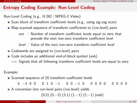
Run-Level Coding (e.g., H.262 | MPEG-2 Video)
Scan block of transform coefficient levels (e.g., using zig-zag scan)
Map scanned sequence of transform coefficients to (run,level) pairs
run : Number of transform coefficient levels equal to zero thatprecede the next non-zero transform coefficient level
level : Value of the next non-zero transform coefficient level
Codewords are assigned to (run,level) pairs
Code includes an additional end-of-block symbol (eob)
=⇒ Signals that all following transform coefficient levels are equal to zero
Example:
Scanned sequence of 20 transform coefficient levels
5 −3 0 0 0 1 0 −1 0 0 −1 0 0 0 0 0 0 0 0 0
A conversion into run-level pairs (run,level) yields
(0,5) (0,−3) (3,1) (1,−1) (2,−1) (eob)
Thomas Wiegand Digital Image Communication 32 / 48
o
Intra-Picture Coding Entropy Coding of Transform Coefficient Levels
Entropy Coding Example: Run-Level-Last Coding
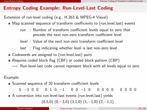
Extension of run-level coding (e.g., H.263 & MPEG-4 Visual)
Map scanned sequence of transform coefficients to (run,level,last) events
run : Number of transform coefficient levels equal to zero thatprecede the next non-zero transform coefficient level
level : Value of the next non-zero transform coefficient level
last : Flag indicating whether level is last non-zero level
Codewords are assigned to (run,level,last) pairs
Requires coded block flag (CBF) or coded block pattern (CBP)
=⇒ Run-level-last code cannot represent block with all levels equal to zero
Example:
Scanned sequence of 20 transform coefficient levels
5 −3 0 0 0 1 0 −1 0 0 −1 0 0 0 0 0 0 0 0 0
A conversion into run-level-last events (run,level,last) yields
(0,5,0) (0,−3,0) (3,1,0) (1,−1,0) (2,−1,1)
Thomas Wiegand Digital Image Communication 33 / 48
o
Intra-Picture Coding Entropy Coding of Transform Coefficient Levels
Entropy Coding Example: CABAC in H.265 | MPEG-H HEVC
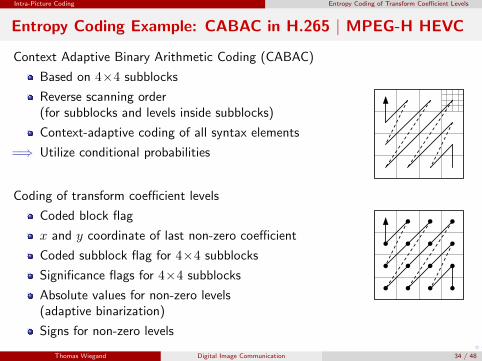
Context Adaptive Binary Arithmetic Coding (CABAC)
Based on 4×4 subblocks
Reverse scanning order(for subblocks and levels inside subblocks)
Context-adaptive coding of all syntax elements
=⇒ Utilize conditional probabilities
Coding of transform coefficient levels
Coded block flag
x and y coordinate of last non-zero coefficient
Coded subblock flag for 4×4 subblocks
Significance flags for 4×4 subblocks
Absolute values for non-zero levels(adaptive binarization)
Signs for non-zero levels
Thomas Wiegand Digital Image Communication 34 / 48
o
Intra-Picture Coding Entropy Coding of Transform Coefficient Levels
Comparison of Entropy Coding Techniques
-20
-10
0
10
20
30
0 10 20 30 40 50 60 70 80
bit-
rate
incr
ease
[%]
bit rate (first-order entropy) [Mbit/s]
Cactus (residual pictures)
run-level coding(H.262 | MPEG-2 Video)
run-level-last coding (MPEG-4 Visual)
CABAC (H.265 | MPEG-H HEVC)-20
-10
0
10
20
30
0 10 20 30 40 50
bit-
rate
incr
ease
[%]
bit rate (first-order entropy) [Mbit/s]
Kimono (residual pictures)
run-level-last coding (MPEG-4 Visual)
CABAC (H.265 | MPEG-H HEVC)
run-level coding (H.262 | MPEG-2 Video)
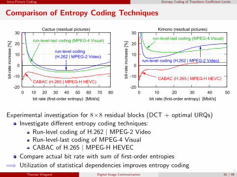
Experimental investigation for 8×8 residual blocks (DCT + optimal URQs)
Investigate different entropy coding techniques:
Run-level coding of H.262 | MPEG-2 VideoRun-level-last coding of MPEG-4 VisualCABAC of H.265 | MPEG-H HEVEC
Compare actual bit rate with sum of first-order entropies
=⇒ Utilization of statistical dependencies improves entropy coding
Thomas Wiegand Digital Image Communication 35 / 48
o
Intra-Picture Coding Intra-Picture Prediction
Intra-Picture Prediction
Transform coding
Typical design:
2D Discrete Cosine Transform of type II (or integer approximation)Scalar quantization: URQs with same quantization step size ∆Entropy coding (employing remaining statistical dependencies)
Can only utilize dependencies within transform blocks
Intra-picture prediction
Can additionally utilize dependencies between transform blocks
Very simple variant (H.262 | MPEG-2 Video):Predict DC coefficient using DC coefficient of previous block
More advanced approaches can significantly increase coding efficiency
Two approaches of intra-picture prediction
Prediction in transform domain
Prediction in spatial domain (before transform coding)
Thomas Wiegand Digital Image Communication 36 / 48
o
Intra-Picture Coding Intra-Picture Prediction
Intra-Picture Prediction in Transform Domain
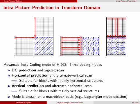
Advanced Intra Coding mode of H.263: Three coding modes
DC prediction and zig-zag scan
Horizontal prediction and alternate-vertical scan
=⇒ Suitable for blocks with mainly horizontal structures
Vertical prediction and alternate-horizontal scan
=⇒ Suitable for blocks with mainly vertical structures
Mode is chosen on a macroblock basis (e.g., Lagrangian mode decision)
Thomas Wiegand Digital Image Communication 37 / 48

o
Intra-Picture Coding Intra-Picture Prediction
Intra Prediction: Transform Domain — Spatial Domain
verticalprediction
intransformdomain
equivalentvertical
predictionin spatialdomain
simplifiedand
improvedvertical
predictionin spatialdomain
Example: Vertical prediction
Transform domain: Predict first row of transform coefficients
Equivalent prediction in spatial domain
sver[x, y] =1
N
N−1∑k=0
s′[x,−1− k]
Simplified prediction in spatial domain
sver[x, y] = s′[−1, y]
Thomas Wiegand Digital Image Communication 38 / 48
o
Intra-Picture Coding Intra-Picture Prediction
Spatial Intra Prediction
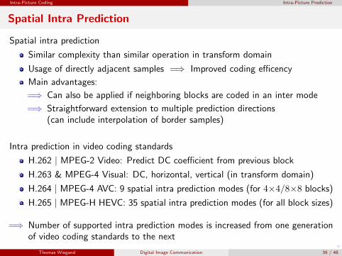
Spatial intra prediction
Similar complexity than similar operation in transform domain
Usage of directly adjacent samples =⇒ Improved coding efficency
Main advantages:
=⇒ Can also be applied if neighboring blocks are coded in an inter mode
=⇒ Straightforward extension to multiple prediction directions(can include interpolation of border samples)
Intra prediction in video coding standards
H.262 | MPEG-2 Video: Predict DC coefficient from previous block
H.263 & MPEG-4 Visual: DC, horizontal, vertical (in transform domain)
H.264 | MPEG-4 AVC: 9 spatial intra prediction modes (for 4×4/8×8 blocks)
H.265 | MPEG-H HEVC: 35 spatial intra prediction modes (for all block sizes)
=⇒ Number of supported intra prediction modes is increased from one generationof video coding standards to the next
Thomas Wiegand Digital Image Communication 39 / 48

o
Intra-Picture Coding Intra-Picture Prediction
Example: Spatial Intra Prediction in H.264 | MPEG-4 AVC
Thomas Wiegand Digital Image Communication 40 / 48
o
Intra-Picture Coding Intra-Picture Prediction
Spatial Intra Prediction — Coding Efficiency
0
10
20
30
40
50
30 32 34 36 38 40
bit-
rate
sav
ing
vs D
C p
red.
[%]
PSNR (Y) [dB]
Cactus (1920×1080, 50 Hz), 8×8 blocks
DC, horizontal, and vertical prediction
9 prediction modes
35 prediction modes
0
10
20
30
40
50
34 36 38 40 42 44
bit-
rate
sav
ing
vs D
C p
red.
[%]
PSNR (Y) [dB]
Kimono (1920×1080, 24 Hz), 8×8 blocks
DC, horizontal, and vertical prediction
9 prediction modes
35 prediction modes
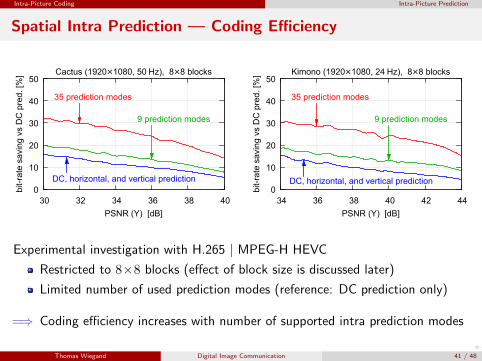
Experimental investigation with H.265 | MPEG-H HEVC
Restricted to 8×8 blocks (effect of block size is discussed later)
Limited number of used prediction modes (reference: DC prediction only)
=⇒ Coding efficiency increases with number of supported intra prediction modes
Thomas Wiegand Digital Image Communication 41 / 48

o
Intra-Picture Coding Block Sizes for Prediction and Transform Coding
Block Sizes for Prediction and Transform Coding
Impact of block size selection for transform coding
Coding efficiency of transform coding typically increases with block size
Coding efficiency improvement becomes small beyond a certain block size
Complexity increases with block size
Impact of block size selection for spatial prediction
Correlation decreases with increasing sample distances
Intra prediction is more effective for smaller block sizes
Side information rate (for intra modes) increases with decreasing block size
Combination of intra prediction and transform coding
Optimal block size depends on actual signal properties
Natural images: Highly non-stationary statistical properties
=⇒ No single optimal block size
=⇒ Adaptive block size selection can improve coding efficiency
Thomas Wiegand Digital Image Communication 42 / 48
o
Intra-Picture Coding Block Sizes for Prediction and Transform Coding
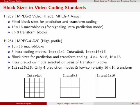
Block Sizes in Video Coding Standards
H.262 | MPEG-2 Video, H.263, MPEG-4 Visual
Fixed block sizes for prediction and transform coding
16×16 macroblocks (for signaling intra prediction mode)
8×8 transform blocks
H.264 | MPEG-4 AVC (High profile)
16×16 macroblocks
3 intra coding modes: Intra4x4, Intra8x8, Intra16x16
Block sizes for prediction and transform coding: 4×4, 8×8, 16×16
Intra prediction mode selected on basis of transform blocks
Intra16x16: Only 4 prediction modes & low-complexity 16×16 transform
Intra4x4 Intra8x8 Intra16x16
Thomas Wiegand Digital Image Communication 43 / 48
o
Intra-Picture Coding Block Sizes for Prediction and Transform Coding
Block Sizes in Video Coding Standards
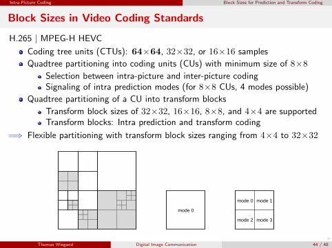
H.265 | MPEG-H HEVC
Coding tree units (CTUs): 64×64, 32×32, or 16×16 samples
Quadtree partitioning into coding units (CUs) with minimum size of 8×8
Selection between intra-picture and inter-picture codingSignaling of intra prediction modes (for 8×8 CUs, 4 modes possible)
Quadtree partitioning of a CU into transform blocks
Transform block sizes of 32×32, 16×16, 8×8, and 4×4 are supportedTransform blocks: Intra prediction and transform coding
=⇒ Flexible partitioning with transform block sizes ranging from 4×4 to 32×32
mode 0
mode 0 mode 1
mode 2 mode 3
Thomas Wiegand Digital Image Communication 44 / 48
o
Intra-Picture Coding Block Sizes for Prediction and Transform Coding
Block Sizes for Intra-Picture Coding — Coding Efficiency
30
32
34
36
38
40
0 20 40 60 80 100
PS
NR
(Y
) [d
B]
bit rate [Mbit/s]
Cactus (1920×1080, 50 Hz), DC prediction
4×4 blocks
8×8 blocks
16×16 blocks
32×32blocks
all block sizes
34
36
38
40
42
44
0 10 20 30 40 50
PS
NR
(Y
) [d
B]
bit rate [Mbit/s]
Kimono (1920×1080, 24 Hz), DC prediction
4×4 blocks
8×8 blocks
16×16 blocks
32×32 blocks
all block sizes
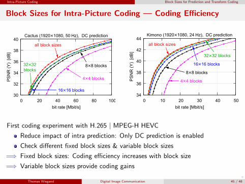
First coding experiment with H.265 | MPEG-H HEVC
Reduce impact of intra prediction: Only DC prediction is enabled
Check different fixed block sizes & variable block sizes
=⇒ Fixed block sizes: Coding efficiency increases with block size
=⇒ Variable block sizes provide coding gains
Thomas Wiegand Digital Image Communication 45 / 48
o
Intra-Picture Coding Block Sizes for Prediction and Transform Coding
Block Sizes for Intra-Picture Coding — Coding Efficiency
30
32
34
36
38
40
0 20 40 60 80 100
PS
NR
(Y
) [d
B]
bit rate [Mbit/s]
Cactus (1920×1080, 50 Hz), all pred. modes
4×4 blocks
8×8 blocks
16×16 blocks
32×32 blocks
all block sizes
34
36
38
40
42
44
0 10 20 30 40 50
PS
NR
(Y
) [d
B]
bit rate [Mbit/s]
Kimono (1920×1080, 24 Hz), all pred. modes
4×4 blocks
8×8 blocks
16×16 blocks
32×32 blocks
all block sizes
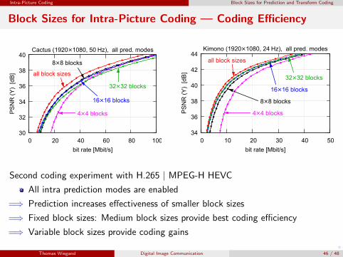
Second coding experiment with H.265 | MPEG-H HEVC
All intra prediction modes are enabled
=⇒ Prediction increases effectiveness of smaller block sizes
=⇒ Fixed block sizes: Medium block sizes provide best coding efficiency
=⇒ Variable block sizes provide coding gains
Thomas Wiegand Digital Image Communication 46 / 48

o
Intra-Picture Coding Block Sizes for Prediction and Transform Coding
Block Sizes for Intra-Picture Coding — Coding Efficiency
0
10
20
30
40
50
30 32 34 36 38 40
bit-
rate
sav
ing
vs 8×
8 bl
ocks
[%]
PSNR (Y) [dB]
Cactus (1920×1080, 50 Hz), all pred. modes
4×4 and 8×8 blocks
4×4, 8×8 blocks,and 16×16 blocks
all block sizes (4×4 to 32×32)
0
10
20
30
40
50
34 36 38 40 42 44
bit-
rate
sav
ing
vs 8×
8 bl
ocks
[%]
PSNR (Y) [dB]
Kimono (1920×1080, 24 Hz), all pred. modes
4×4 and 8×8 blocks
4×4, 8×8 blocks,and 16×16 blocks
all block sizes (4×4 to 32×32)
Third coding experiment with H.265 | MPEG-H HEVC
All intra prediction modes are enabled
Start with 8×8 blocks and successively enable additional block sizes
=⇒ Additional block sizes provide coding efficiency improvements
=⇒ Beside intra-picture prediction, the support of additional block sizes is a mainfactor for the improvement in intra-picture coding
Thomas Wiegand Digital Image Communication 47 / 48

o
Intra-Picture Coding Block Sizes for Prediction and Transform Coding
Summary
Transform coding of sample blocks
Separable orthogonal transform: DCT or integer approximation
Scalar quantization: URQs with same quantization step size ∆
Entropy coding: Utilize remaining dependencies between quantization indexes
Intra-picture prediction
Utilize dependencies between transform blocks
Two methods: Prediction in transform domain or spatial domain
Spatial prediction: Straightforward realization of multiple prediction modes
Coding efficiency typically increases with number of supported intra modes
Block sizes for intra prediction and transform coding
Determine efficiency of prediction and transform coding
Non-stationary character of natural images =⇒ Variable block sizes
Simple and flexible partitioning: Quadtree-based approaches
Variable block sizes significantly increase coding efficiency
Thomas Wiegand Digital Image Communication 48 / 48