Intra-Household Allocation of Calorie Intake

Manoranjan Pal&

Premananda Bharati

Indian Statistical InstituteEmail: mano@isical.ac.in, manoranjanpal@hotmail.com,

Ph: (Off.) (+91) (33) 25752521/2/0, (M) 9433563962.

Preliminaries: Regression

• A variable is predicted using one or more variables.

• It can not be predicted exactly.

• We minimize the prediction error to estimate the parameters.

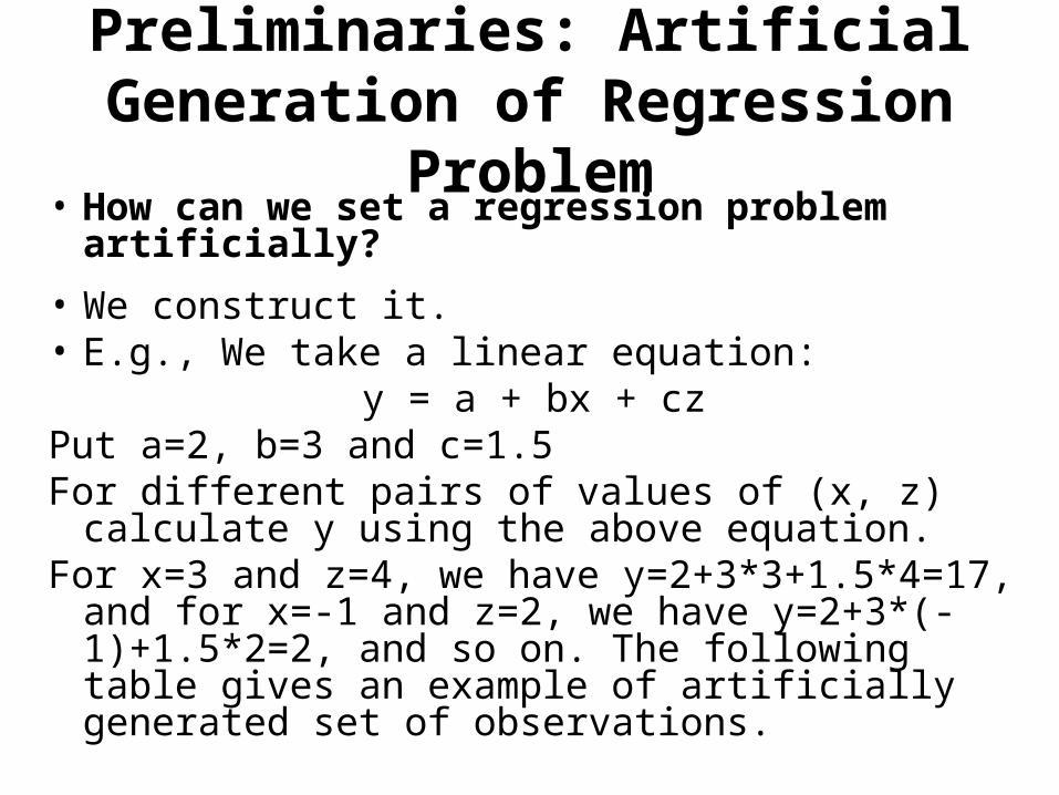
Preliminaries: Artificial Generation of Regression Problem

• How can we set a regression problem artificially?

• We construct it.• E.g., We take a linear equation:

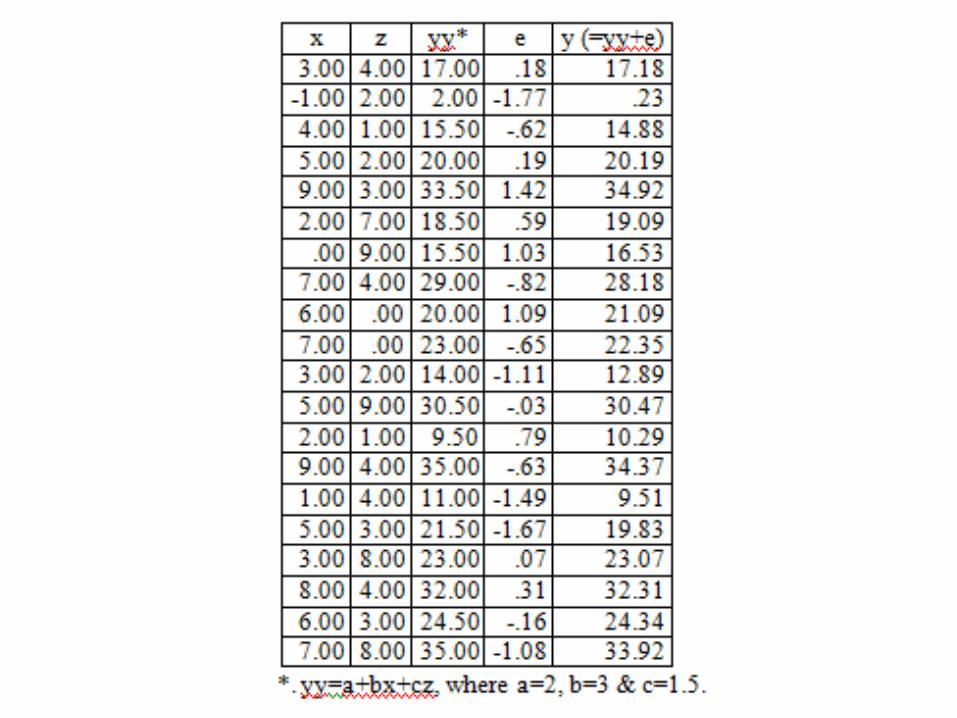
y = a + bx + czPut a=2, b=3 and c=1.5For different pairs of values of (x, z) calculate y using

the above equation. For x=3 and z=4, we have y=2+3*3+1.5*4=17, and

for x=-1 and z=2, we have y=2+3*(-1)+1.5*2=2, and so on. The following table gives an example of artificially generated set of observations.

Preliminaries: The Regression Estimates

• The regression estimates found in the above artificial example are

a = 1.355b = 3.055

and c = 1.546.

• The estimate of the intercept term differed from the actual value more than those of b and c. This is because the sum of the error terms was not close to ‘0’ and we have assumption that E(e)=0.

Preliminaries: Discussions

• In the artificial regression the estimate of ‘a’ has more standard error than those of ‘b’ and ‘c’. I.e., estimates of ‘b’ and ‘c’ are more robust.

• The regression technique can be used to estimate the unknown parameters in identities of the form

y = ∑bixi,

where bis are unknown. These identities may be termed as Regression Decomposition Identities.

Preliminaries: Regression Decomposition Identities

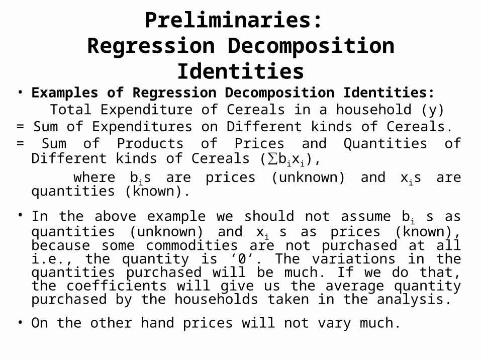
• Examples of Regression Decomposition Identities: Total Expenditure of Cereals in a household (y)= Sum of Expenditures on Different kinds of Cereals.= Sum of Products of Prices and Quantities of Different kinds of

Cereals (∑bixi), where bis are prices (unknown) and xis are quantities (known).

• In the above example we should not assume bi s as quantities (unknown) and xi s as prices (known), because some commodities are not purchased at all i.e., the quantity is ‘0’. The variations in the quantities purchased will be much. If we do that, the coefficients will give us the average quantity purchased by the households taken in the analysis.

• On the other hand prices will not vary much.

Preliminaries: Regression Decomposition Identities

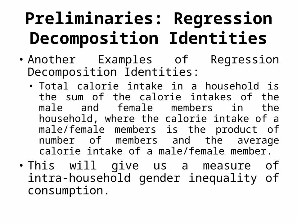
• Another Examples of Regression Decomposition Identities:• Total calorie intake in a household is the sum of

the calorie intakes of the male and female members in the household, where the calorie intake of a male/female members is the product of number of members and the average calorie intake of a male/female member.

• This will give us a measure of intra-household gender inequality of consumption.

Preliminaries: Regression Decomposition Identities

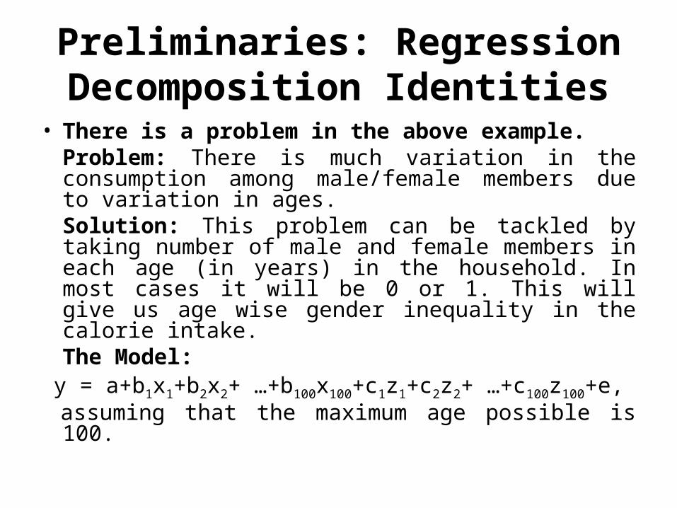
• There is a problem in the above example.Problem: There is much variation in the consumption among male/female members due to variation in ages.Solution: This problem can be tackled by taking number of male and female members in each age (in years) in the household. In most cases it will be 0 or 1. This will give us age wise gender inequality in the calorie intake.The Model: y = a+b1x1+b2x2+ …+b100x100+c1z1+c2z2+ …+c100z100+e,

assuming that the maximum age possible is 100.

Preliminaries: Regression Decomposition Identities

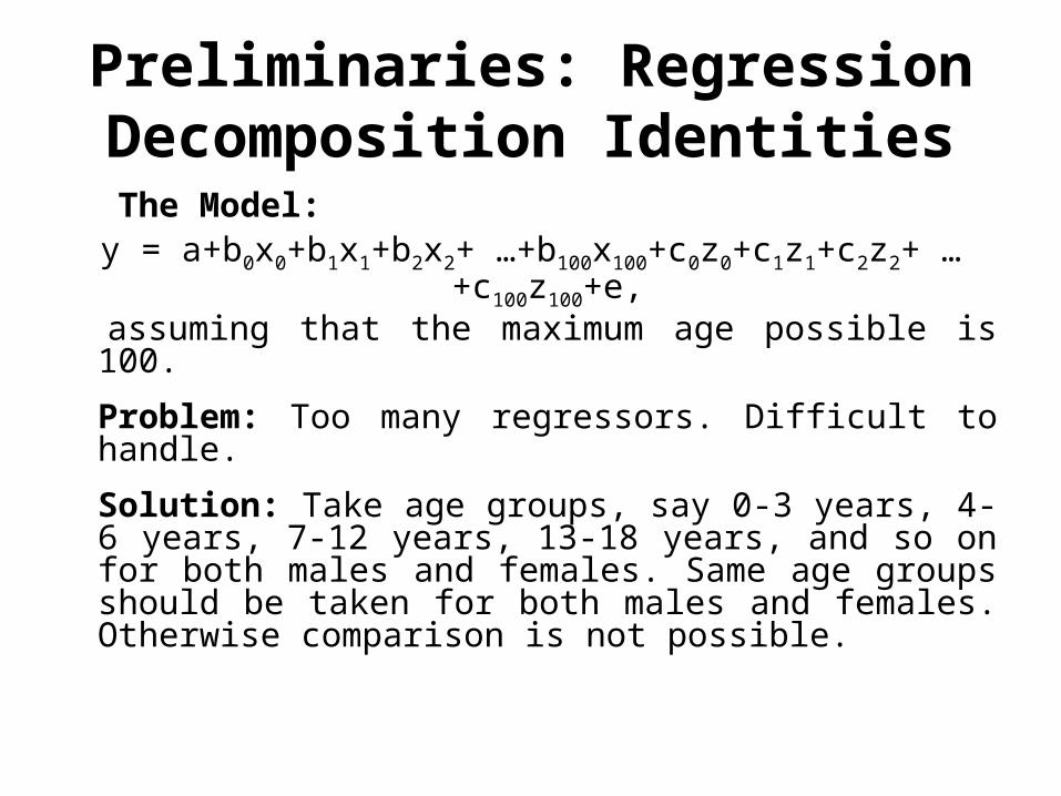
The Model: y = a+b0x0+b1x1+b2x2+ …+b100x100+c0z0+c1z1+c2z2+ …

+c100z100+e, assuming that the maximum age possible is 100.

Problem: Too many regressors. Difficult to handle.

Solution: Take age groups, say 0-3 years, 4-6 years, 7-12 years, 13-18 years, and so on for both males and females. Same age groups should be taken for both males and females. Otherwise comparison is not possible.

Aim of this Paper

We are interested in knowing whether there is any difference in the consumption of food between male and female members in the households in India.

The consumption of food is summarized here through the mean calorie consumption of male and female members in each Age Group.

Human Energy Requirements

“Energy requirement is the amount of food energy needed to balance energy expenditure in order to maintain body size, body composition and a level of necessary and desirable physical activity consistent with long-term good health.”

However since there are interpersonal variations, the mean level of dietary energy intake of the healthy, well-nourished individuals who constitute that group has been recommended as the energy requirement for the population group.

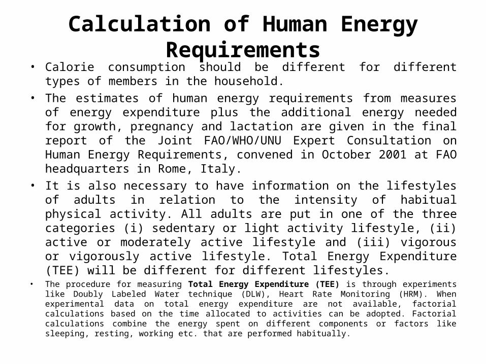
Calculation of Human Energy Requirements• Calorie consumption should be different for different types of members in

the household.

• The estimates of human energy requirements from measures of energy expenditure plus the additional energy needed for growth, pregnancy and lactation are given in the final report of the Joint FAO/WHO/UNU Expert Consultation on Human Energy Requirements, convened in October 2001 at FAO headquarters in Rome, Italy.

• It is also necessary to have information on the lifestyles of adults in relation to the intensity of habitual physical activity. All adults are put in one of the three categories (i) sedentary or light activity lifestyle, (ii) active or moderately active lifestyle and (iii) vigorous or vigorously active lifestyle. Total Energy Expenditure (TEE) will be different for different lifestyles.

• The procedure for measuring Total Energy Expenditure (TEE) is through experiments like Doubly Labeled Water technique (DLW), Heart Rate Monitoring (HRM). When experimental data on total energy expenditure are not available, factorial calculations based on the time allocated to activities can be adopted. Factorial calculations combine the energy spent on different components or factors like sleeping, resting, working etc. that are performed habitually.

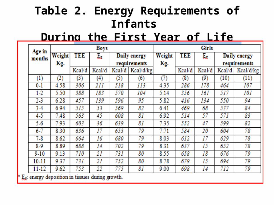
Table 2. Energy Requirements of Infants During the First Year of Life

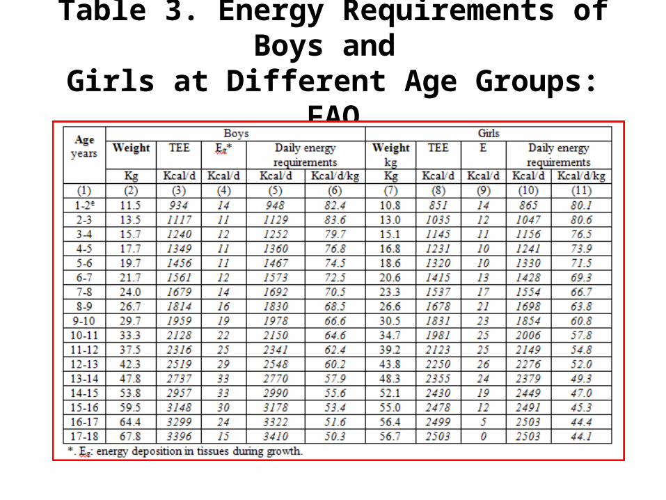
Table 3. Energy Requirements of Boys and Girls at Different Age Groups: FAO

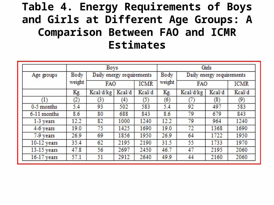
Table 4. Energy Requirements of Boys and Girls at Different Age Groups: A Comparison Between FAO

and ICMR Estimates

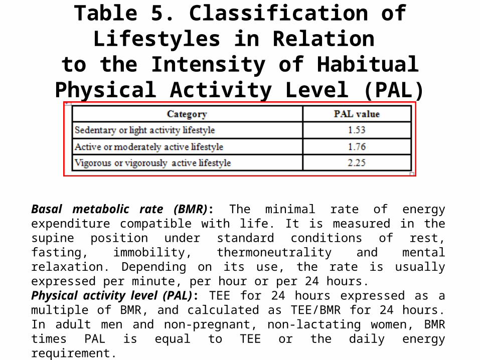
Table 5. Classification of Lifestyles in Relation

to the Intensity of Habitual Physical Activity Level (PAL)

Basal metabolic rate (BMR): The minimal rate of energy expenditure compatible with life. It is measured in the supine position under standard conditions of rest, fasting, immobility, thermoneutrality and mental relaxation. Depending on its use, the rate is usually expressed per minute, per hour or per 24 hours.Physical activity level (PAL): TEE for 24 hours expressed as a multiple of BMR, and calculated as TEE/BMR for 24 hours. In adult men and non-pregnant, non-lactating women, BMR times PAL is equal to TEE or the daily energy requirement.

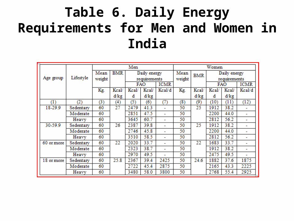
Table 6. Daily Energy Requirements for Men and Women in India

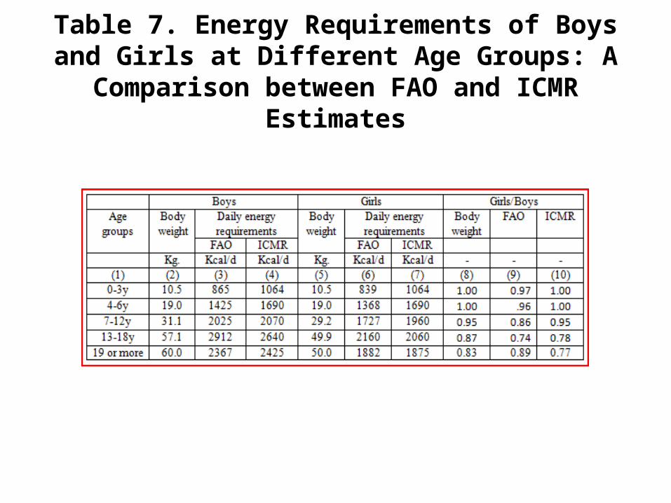
Table 7. Energy Requirements of Boys and Girls at Different Age Groups: A Comparison between FAO

and ICMR Estimates

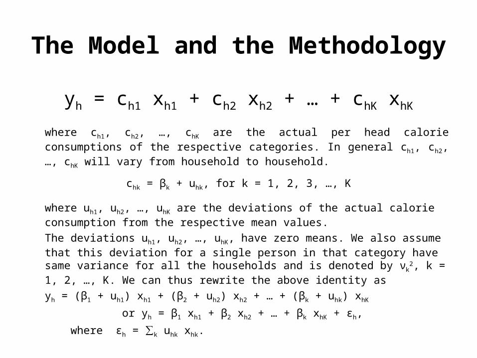
The Model and the Methodology

yh = ch1 xh1 + ch2 xh2 + … + chK xhK

where ch1, ch2, …, chK are the actual per head calorie consumptions of the respective categories. In general ch1, ch2, …, chK will vary from household to household.

chk = βk + uhk, for k = 1, 2, 3, …, K

where uh1, uh2, …, uhK are the deviations of the actual calorie consumption from the respective mean values.

The deviations uh1, uh2, …, uhK, have zero means. We also assume that this deviation for a single person in that category have same variance for all the households and is denoted by νk

2, k = 1, 2, …, K. We can thus rewrite the above identity as

yh = (β1 + uh1) xh1 + (β2 + uh2) xh2 + … + (βk + uhk) xhK

or yh = β1 xh1 + β2 xh2 + … + βk xhK + εh,

where εh = ∑k uhk xhk.

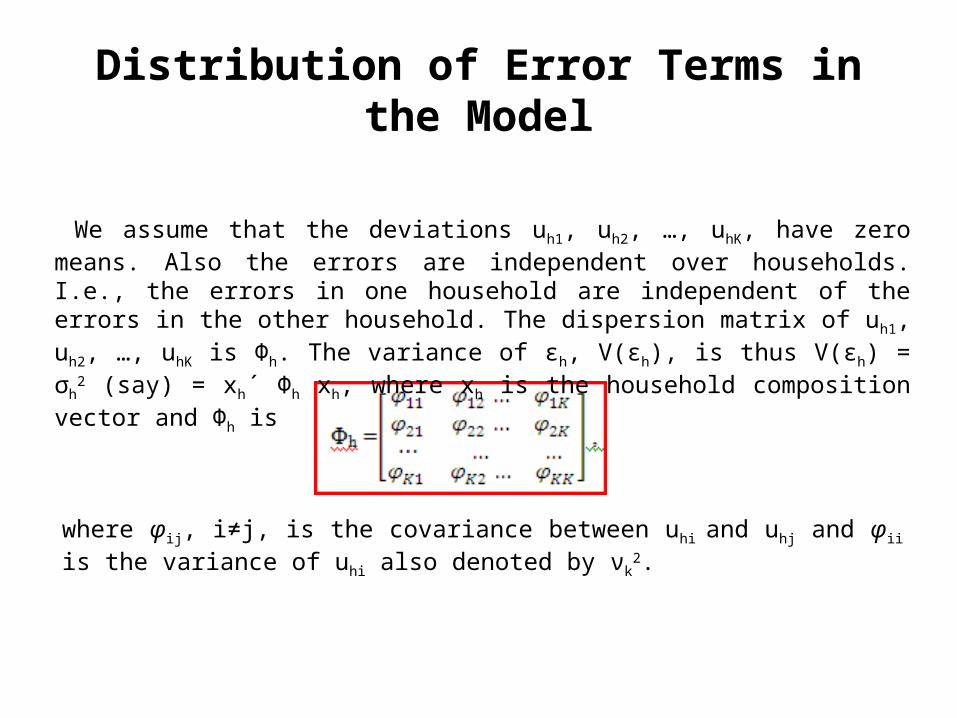
Distribution of Error Terms in the Model

We assume that the deviations uh1, uh2, …, uhK, have zero means. Also the errors are independent over households. I.e., the errors in one household are independent of the errors in the other household. The dispersion matrix of uh1, uh2, …, uhK is Φh. The variance of εh, V(εh), is thus V(εh) = σh

2 (say) = xh´ Φh xh, where xh is the household composition vector and Φh is

where φij, i≠j, is the covariance between uhi and uhj and φii is the variance of uhi also denoted by νk

2.

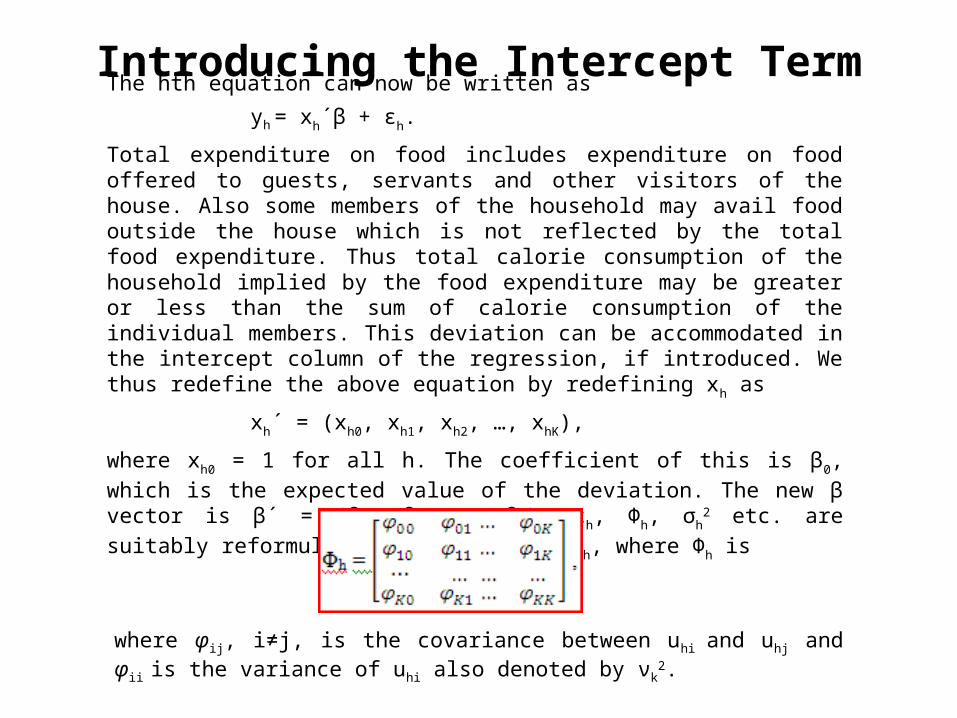
Introducing the Intercept Term

The hth equation can now be written as

yh = xh´β + εh.

Total expenditure on food includes expenditure on food offered to guests, servants and other visitors of the house. Also some members of the household may avail food outside the house which is not reflected by the total food expenditure. Thus total calorie consumption of the household implied by the food expenditure may be greater or less than the sum of calorie consumption of the individual members. This deviation can be accommodated in the intercept column of the regression, if introduced. We thus redefine the above equation by redefining xh as

xh´ = (xh0, xh1, xh2, …, xhK),

where xh0 = 1 for all h. The coefficient of this is β0, which is the expected value of the

deviation. The new β vector is β´ = (β0, β1, …, βK). εh, Φh, σh2 etc. are suitably

reformulated as σh2 = xh´ Φh xh, where Φh is

where φij, i≠j, is the covariance between uhi and uhj and φii is the variance of uhi also denoted by νk

2.

The Regression Equation

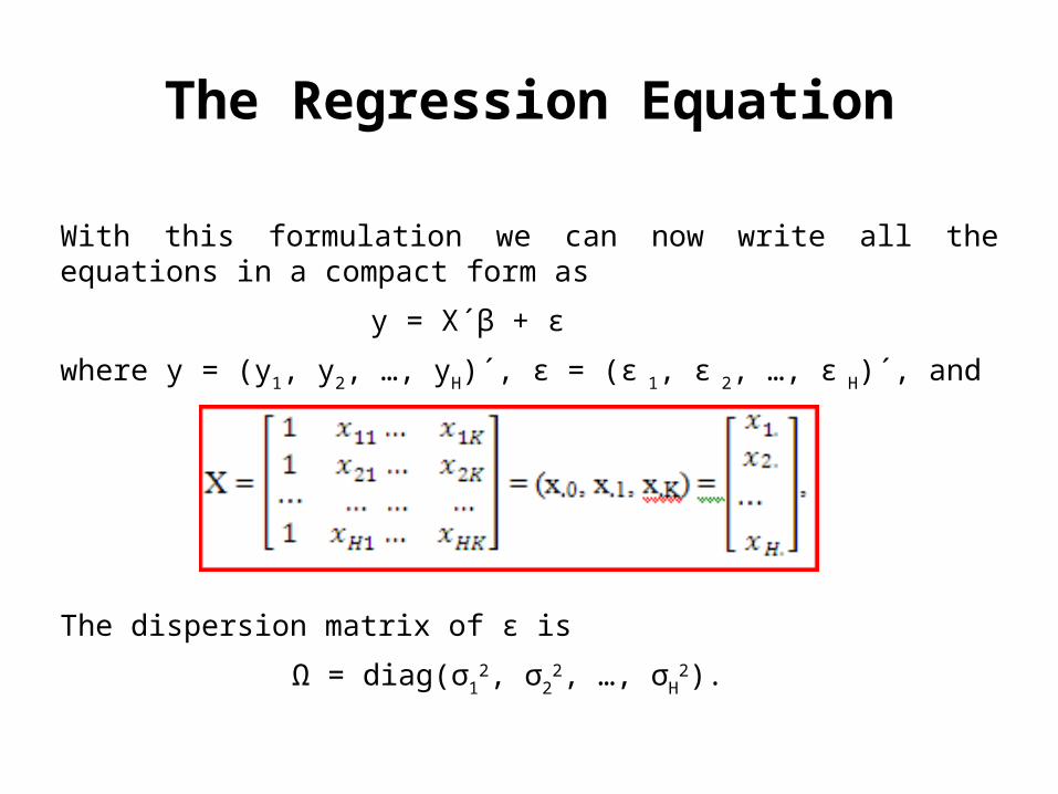
With this formulation we can now write all the equations in a compact form as

y = X´β + ε

where y = (y1, y2, …, yH)´, ε = (ε 1, ε 2, …, ε H)´, and

The dispersion matrix of ε is

Ω = diag(σ12, σ2

2, …, σH2).

Interpretation of the Regression Coefficients

• Each element in β gives the expected amount of calorie consumption for a member in the respective category.

• This may also be interpreted as the increase in the average amount of calorie consumption due to increase by one person in the respective category.

• Usually in regression analysis one can give both the interpretations of the estimated coefficient if the intercept term is not significant. Interestingly, in this case, both the interpretations are plausible even if the intercept term is significant i.e., the sum of individual average calories is not the total calorie on the average.

• If the intercept term is positive, it means that there is extra consumption, possibly by guests or servants for many of the households which outweighed the consumption of food by the members of the households outside the house. If it is negative the interpretation is the other way round.

• The variable associated with the intercept term always takes value 1. Thus it may be interpreted as a ‘ghost’ member in the household which may consume or produce extra calories for consumption of other members.

Estimation of Parameters

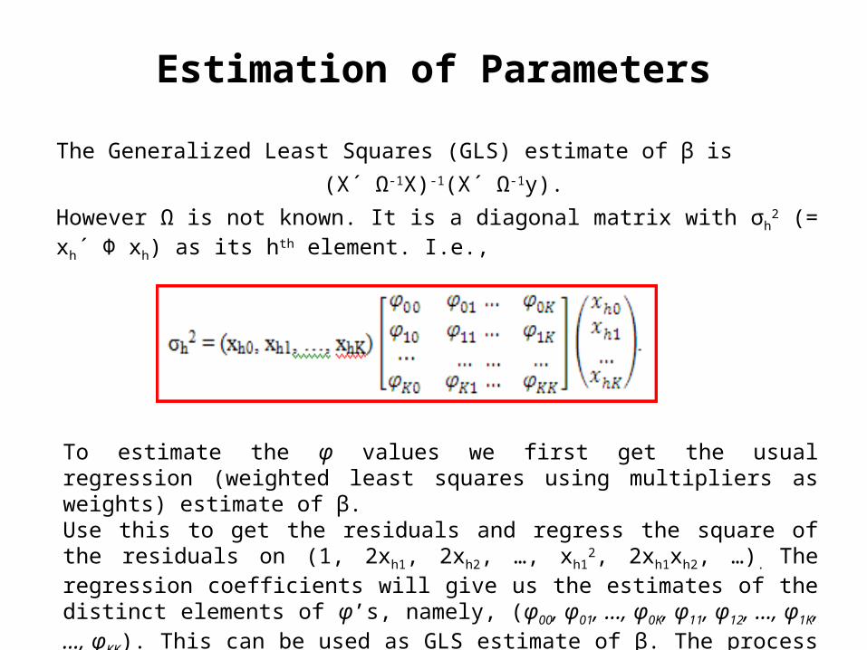
The Generalized Least Squares (GLS) estimate of β is

(X´ Ω-1X)-1(X´ Ω-1y).

However Ω is not known. It is a diagonal matrix with σh2 (= xh´ Φ xh) as its hth element.

I.e.,

To estimate the φ values we first get the usual regression (weighted least squares using multipliers as weights) estimate of β.Use this to get the residuals and regress the square of the residuals on (1, 2xh1, 2xh2, …, xh1

2, 2xh1xh2, …). The regression coefficients will give us the estimates of the distinct elements of φ’s, namely, (φ00, φ01, …, φ0K, φ11, φ12, …, φ1K, …, φKK). This can be used as GLS estimate of β. The process can be repeated until convergence up to desired level of precision.

The Proposed Estimation Procedure

• The non-negativeness of the estimated value of σh2 for each h

is not guaranteed because the estimated value of Φ may not be nonnegative definite. It was in fact found to be so with our consumption data of 61st round of NSSO. Deleting the data associated with negative σh

2 did not help. There were further some negative σh

2 and the process did not end quickly.

• To overcome this problem we have taken Φ to be diagonal with only φ11, φ22, …, φKK. Thus we regressed the square of the residuals on xh1

2, xh22, …, xhK

2. All the coefficients of xh12, xh2

2, …, xhK

2, this time, were positive for most of the subsets of data considered for our analysis. For the few cases where all the coefficients were not found to be positive, we deleted a very few observations to achieve the desired result.

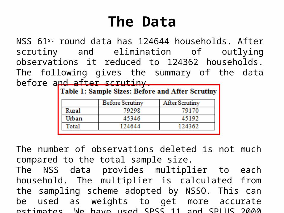
The Data

NSS 61st round data has 124644 households. After scrutiny and elimination of outlying observations it reduced to 124362 households. The following gives the summary of the data before and after scrutiny.

The number of observations deleted is not much compared to the total sample size.The NSS data provides multiplier to each household. The multiplier is calculated from the sampling scheme adopted by NSSO. This can be used as weights to get more accurate estimates. We have used SPSS 11 and SPLUS 2000 for our calculations.

Three Types of Estimation Procedures

• According to the Table 8, coefficients associated with the male members have higher values than those of the female members in most of the cases .

• The estimates varied to some extent over the three types of estimation method.

• The coefficients, i.e., mean consumption of calories, decrease for most especially among members in the lower age groups when we switch to better estimation procedure. However, the mean calorie consumptions for female members remain less than those of male members.

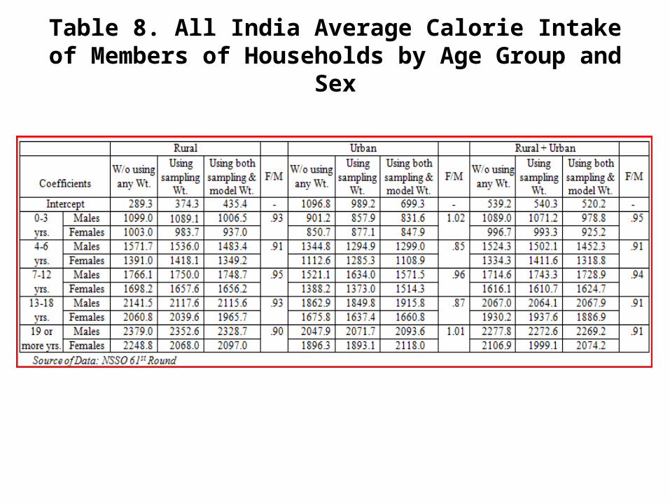
Table 8. All India Average Calorie Intake of Members of Households by Age Group and Sex

Comparison of Our Estimates With FAO and ICMR Norms

• It should be remembered here that the calorie norms of female members given by FAO and ICMR are also less than or equal to those of corresponding male members. So it is difficult to say whether the differences in the calorie consumption between male and female members are as expected or due to gender inequality without comparing these ratios. The comparison is given in the Table 12.

• The gender ratios of the proposed model are seen to be less than the gender ratios found from the norms given by FAO and ICMR among members in the lower age groups and higher among the members in the higher age groups and adults.

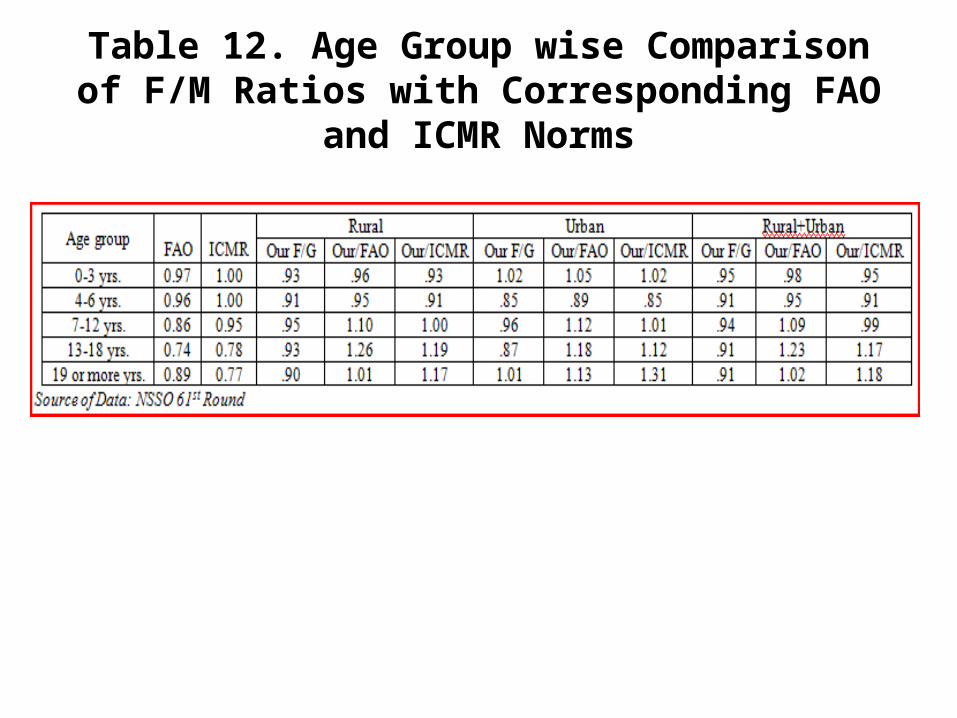
Table 12. Age Group wise Comparison of F/M Ratios with Corresponding FAO and ICMR Norms

Results by Expenditure Groups

• It is felt that the treatment on the members would be different for different income/expenditure levels. We grouped the households into 12 expenditure groups. Group 1 has the lowest and the Group 12 has the highest per capita expenditures. Rural and urban expenditure groups are different.

• The groups are same as the ones taken by NSSO. • The results of the regression analysis are much different now. This time all

the coefficients have increased substantially. This is seen more among the members in the lower Age Groups and in the households with low per capita expenditures. The intercept terms are found to be very small or negative for the lower expenditure groups. This signifies that some consumptions were not taken into account for the lower expenditure group households. The members consumed food outside the house or received food in kind which have not been reported. Similarly, by the same logic, because of high positive values of the intercept terms, it can be concluded that some expenditure on food have been incurred by higher expenditure group households and possibly consumed by members from outside the households which have not been reported.

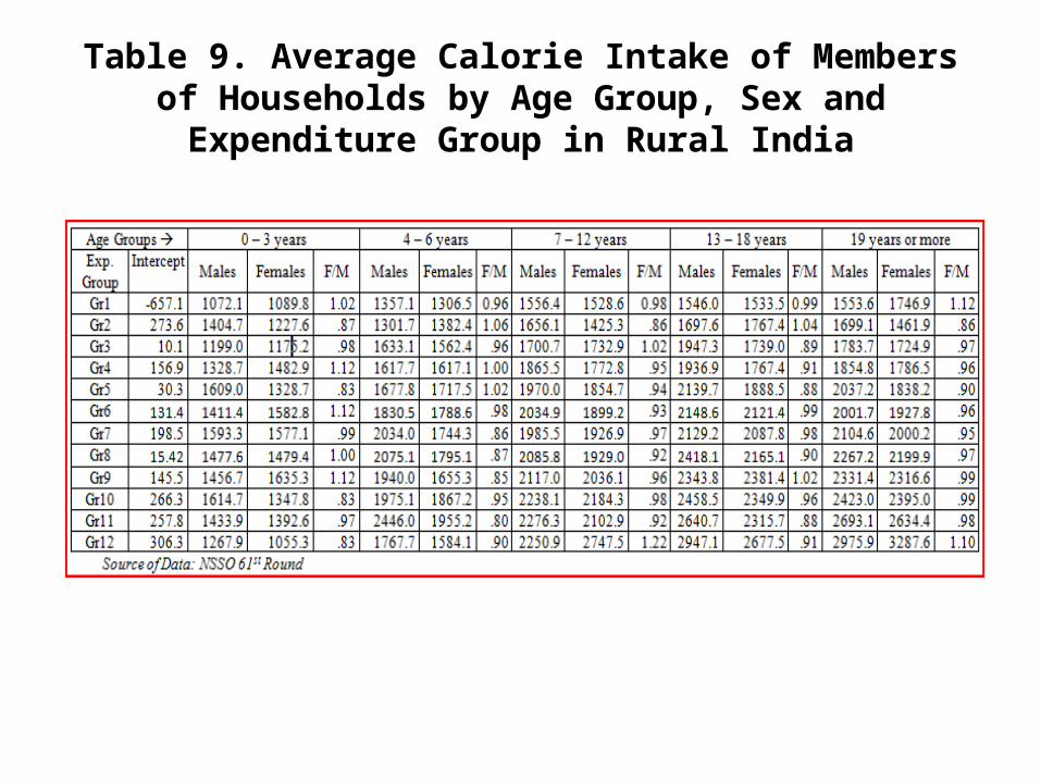
Table 9. Average Calorie Intake of Members of Households by Age Group, Sex and Expenditure Group in Rural India

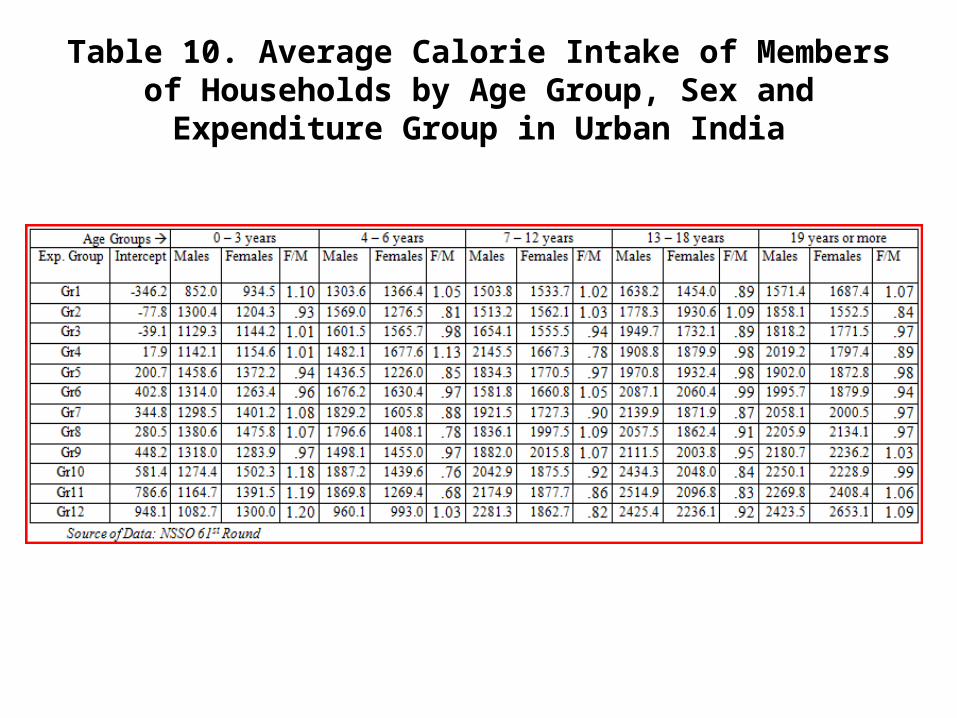
Table 10. Average Calorie Intake of Members of Households by Age Group, Sex and Expenditure Group in Urban India

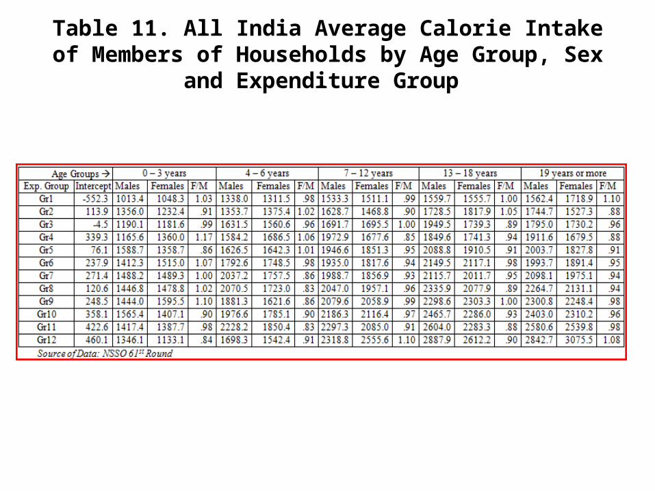
Table 11. All India Average Calorie Intake of Members of Households by Age Group, Sex and Expenditure Group

Results

• The consumption ratios between female and male members are found to be more or less same for all age groups for each expenditure class. Most of the ratios are less than 1. Number of expenditure groups with ratio more than 1 was more among the lower Age Group members especially in Urban India.

The Expenditure Group Wise Regression Results

• The Expenditure Group wise regression results and ratios relative to those of FAO and ICMR are given in Tables 13 through 15. The Gender ratios are found to be more than the gender ratios obtained from the FAO and ICMR norms for most cases. Among the adults and the members in the Age Group 13-18 years it is found to be true for almost cent percent. Even among the lower Age Group members our estimates of the ratios are seen to be more than the corresponding ratios of FAO and ICMR in almost half of the cases.

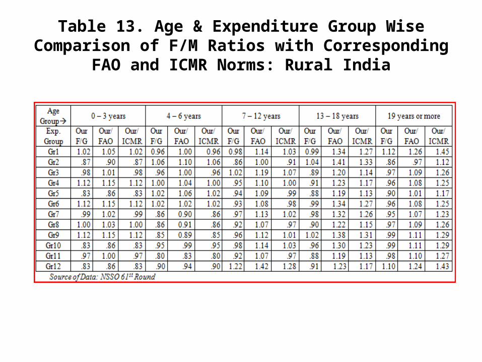
Table 13. Age & Expenditure Group Wise Comparison of F/M Ratios with Corresponding FAO and ICMR Norms:

Rural India

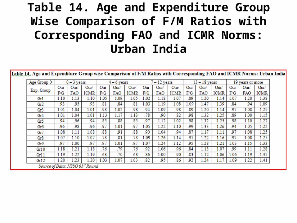
Table 14. Age and Expenditure Group Wise Comparison of F/M Ratios with Corresponding FAO

and ICMR Norms: Urban India

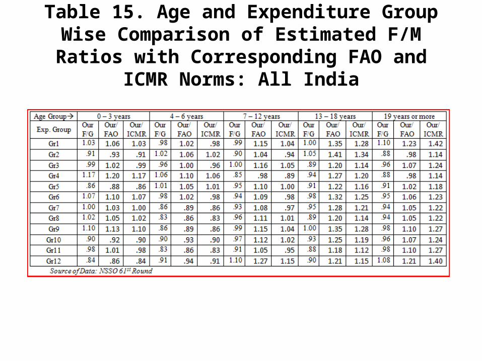
Table 15. Age and Expenditure Group Wise Comparison of Estimated F/M Ratios with

Corresponding FAO and ICMR Norms: All India

Conclusions

• To conclude, the present data do not give any indication of inequality against female members in the households at all levels of income except for the Age Group 4-6 years at high income levels.

• On the contrary the results indicate that the gender inequality may be present against male members especially the grown up members in the households.

• The differences in the ratios in the Age Group 4-6 years between our estimates and those of FAO and ICMR should be further looked into.

• There are however certain limitations in our analysis.

(i) We have not considered the activity patterns of the adult members in the households. For calculations of calorie norms the adults are usually put in one of the three groups according to the activity pattern or life style – sedentary life style, moderately active life style and vigorously active life style.

(ii) Since male members are more actively involved, it is expected that if we consider the activity patterns, the results will indicate more discrimination against male members in the households. Whether one should term it as discrimination or self imposed less consumption by the male members remains a question.

Thank you