Interpolation-Based Model Order Reduction for Polynomial

INTERPOLATION-BASED MODEL ORDER REDUCTION FORPOLYNOMIAL PARAMETRIC SYSTEMS∗

PETER BENNER† AND PAWAN GOYAL‡

Abstract. In this work, we investigate a model order reduction scheme for polynomial paramet-ric systems. We begin with defining the generalized multivariate transfer functions for the system.Based on this, we aim at constructing a reduced-order system, interpolating the defined generalizedtransfer functions at a given set of interpolation points. Furthermore, we provide a method, inspiredby the Loewner approach for linear and (quadratic-)bilinear systems, to determine a good-qualityreduced-order system in an automatic way. We also discuss the computational issues related tothe proposed method and a potential application of CUR matrix approximation in order to furtherspeed-up simulations of reduced-order systems. We test the efficiency of the proposed methods viaseveral numerical examples.

Key words. Model order reduction, interpolation, tensor algebra, matricization, polynomialdynamical systems, parametric systems, transfer functions.

AMS subject classifications. 15A69, 34C20, 41A05, 49M05, 93A15, 93C10, 93C15

1. Introduction. An accurate solution of time-dependent partial differentialequations (PDEs), or ordinary differential equations (ODEs), or a combination ofboth requires a fine spatial discretization of the governing equations. This leads to alarge number of equations, thus a high-dimensional system. This inevitably imposesa huge burden on computational resources, and more often than not, it is almostimpossible to make use of such high-dimensional systems in engineering problem like,e.g., optimization or control. A way to resolve this issue is to construct a reduced-order system or a low-dimensional model, replicating the important dynamics of theoriginal system.

In this paper, we focus on parametric polynomial systems of the form:

(1.1)

E(p)x(t,p) = A(p)x(t,p) +

d∑ξ=2

Hξ(p)x ξ (t,p) +

d∑η=1

Nη(p) (u(t)⊗ xη (t,p))

+B(p)u(t), x(0,p) = 0,

y(t,p) = C(p)x(t,p),

where E(p), A(p) ∈ Rn×n, B(p) ∈ Rn×m, C(p) ∈ Rq×n, Hξ(p) ∈ Rn×nξ , ξ ∈{2, . . . , d}, Nη(p) ∈ Rn×m·nη , η ∈ {1, . . . , d}; the state, input and output vectorsare x(t) ∈ Rn, u(t) ∈ Rm and y(t) ∈ Rq, respectively; x ξ := x⊗ · · · ⊗ x︸︷︷︸

ξ−times

and the

parameter vector is denoted p ∈ Rnp . Since the system (1.1) has polynomial terms ofthe order up to d, we refer to it as a d-th order polynomial system. The system (1.1)lies in n-dimensional Euclidean space and generally, n is in O

(105)−O

(106). Due to

the computational burden mentioned above, we seek to construct a low-dimensionalsystem, having the same structure as (1.1), which captures the dynamics of the originalsystem (1.1) for any given input u(t) and parameter p in a desired domain.

∗Submitted to the editors April 29, 2019.†Max Planck Institute for Dynamics of Complex Technical Systems, Sandtorstraße 1, 39106

Magdeburg, Germany ([email protected]).‡Corresponding author. Max Planck Institute for Dynamics of Complex Technical Systems, Sand-

torstraße 1, 39106 Magdeburg, Germany ([email protected]).

1

arX

iv:1

904.

1189

1v1

[m

ath.

NA

] 2

6 A

pr 2

019

mailto:[email protected]

mailto:[email protected]

2 PETER BENNER, AND PAWAN GOYAL

Many of the widely used methods in model order reduction (MOR) to constructlow-dimensional models for (parametric) nonlinear systems are based on snapshots.This means that the state vector x at time t needs to be evaluated for a given inputand parameter. In this category, proper orthogonal decomposition is arguably themost favored method. This relies on determining the dominant subspace for the statevectors through singular value decomposition (SVD) of the collected snapshots, whichis generally followed by computing a reduced-order system via Galerkin projection.For more details, we refer to [17]. For nonlinear systems, it is often combined withhyper-reduction methods such as EIM [6] and DEIM [13] to further reduce computa-tional costs related to the reduced nonlinear terms. Another widely known method inthis category is the trajectory piecewise linear method, in which a nonlinear systemis approximated by a weighted sum of linearized systems (linearized along the trajec-tory). Then, each linear system is reduced using popular methods for linear systemssuch as balanced truncation or iterative methods, see, e.g. [3, 9, 12, 18]. Moreover,reduced basis methods, which are also snapshots-based methods, have been success-fully applied to several nonlinear parametric systems, see, e.g., [25]. Although thesemethods have been very successful, they share a common drawback of being depen-dent on snapshots, or in other words, simulations for given inputs and parameters.Hence, it may become harder to obtain a reduced-order system to use e.g., in control.

In this work, we rather focus on MOR methods, allowing us to determine reduced-order systems without any prior knowledge of inputs. There are, broadly speaking, twotypes of such methods, namely interpolation-based approaches and balanced trunca-tion. Recently, there have been significant efforts to extend these methods from linearto special classes of non-parametric polynomial systems, namely bilinear systems, andquadratic-bilinear systems, see, e.g., [4, 7, 8, 10, 11, 15]. For parametric nonlinearsystems, there has been a very recent work for bilinear parametric systems [26], wherethe construction of an interpolating reduced system has been proposed for a given setof interpolation points, and such a problem for quadratic-bilinear parametric systemsstill remains to be studied.

In this paper, we investigate an interpolation-based MOR scheme to obtain areduced-order system for the parametric system (1.1). For this, we first define gener-alized transfer functions for the system (1.1). Based on this, we aim at constructing areduced-order system such that its generalized transfer functions interpolate those ofthe original system at a given set of interpolation points for the frequency and param-eters. Furthermore, we propose a scheme, inspired by the Loewner approach for linearand (quadratic-)bilinear systems [4, 15], thus leading to an algorithm that allows us toconstruct a good quality reduced-order system in an automatic fashion. Furthermore,we discuss related computational aspects and an application of pseudo-skeletal matrixapproximation, the so-called CUR, to further reduce the computational complexityrelated to the reduced nonlinear terms.

The remaining structure of the paper is as follows. In the following section, wediscuss polynomialization of nonlinear systems and recap some basic concepts fromtensor algebra. In Section 3, we present the generalized transfer functions corre-sponding to (1.1) for a fixed parameter vector and discuss the construction of aninterpolating reduced-order system using Petrov-Galerkin projection. Based on this,we propose an algorithm which allows us to determine a good quality reduced-ordersystem in an automatic fashion. In Section 4, we discuss the related computationalaspects and investigate an application of CUR matrix approximation to further reducethe complexity of the reduced nonlinear terms. In the subsequent section, we extendthe proposed method to polynomial parametric systems. In Section 6, we illustrate

INTERPOLATION-BASED MOR SCHEME FOR POLYNOMIAL SYSTEMS 3

the efficiency of the proposed algorithms by means of two benchmark problems andtheir variants. We conclude the paper with a summary of our contributions and futureperspectives.

We make use of the following notation in the paper:• orth(): it returns an orthonormal basis of a given matrix.• The Hadamard product and Kronecker product are denoted by ‘◦’ and ‘⊗’,

respectively.• Using MATLAB® notation, A(:, 1:r) denotes the first r columns of the matrixA, and A(i, j) is the (i, j)th element of the matrix A.

• Im is the identity matrix of size m×m.• V ξ is a short-hand notation for V ⊗ · · · ⊗ V︸︷︷︸

ξ−times

, where V is a vector/matrix.

2. Polynomialization of Nonlinear Systems and Tensor Algebra. In thissection, we recap two topics. We begin with the polynomialization of nonlinear sys-tems.

2.1. Polynomialization of nonlinear systems. A class of nonlinear systems,containing nonlinear terms such as exponential, trigonometric, rational, can be rewrit-ten as a polynomial system (1.1), by introducing some auxiliary variables. This pro-cess is very closely related to the McCormick relaxation, used in nonconvex opti-mization [24]. In the recent past, due to advances in the methodologies for MORfor quadratic-bilinear (QB) systems, there has been a substantial focus on rewriting anonlinear system into the QB form. However, in the subsection, we will illustrate withan example how a polynomialization of a nonlinear system is done by introducing lessauxiliary variables as compared to its quadratic-bilinearization.

An illustrative example. Let us consider the following one-dimensional non-linear ODE:

x(t) = −x(t)− x3(t) · e−x(t) + u(t),(2.1a)

y(t) = x(t).(2.1b)

Now, we seek to rewrite the system (2.1) as a polynomial system via polynomializa-tion. For this, we introduce an auxiliary variable as z(t) := e−x(t) and derive thecorresponding differential equation. That is

z(t) = −e−x(t)x(t) = −z(t)(−x(t)− x3(t)z(t) + u(t)

).

Thus, we can equivalently write the input-output system (2.1) as follows:[x(t)z(t)

]=

[−x(t)

0

]+

[0

x(t)z(t)

]−[x3(t)z(t)

0

]+

[0

x3(t)z2(t)

]−[

0z(t)

]u(t) +

[u(t)

0

],

y(t) =[1 0

] [x(t)z(t)

].

As can be seen, the system (2.1), which has cubic exponential nonlinearity, can berewritten into a polynomial system (3.1) of order 5 by introducing a single variable.However, if one aims at rewriting the system into the QB form, then we need tointroduce at least 3 more auxiliary variables, which somehow also makes the resultingsystem even more complicated, hence, also impeding its model reduction. Therefore,it is advantageous to work with the polynomial system of order 5 and thus, we aimat reducing polynomial systems with MOR schemes for polynomial systems.


Figure 2.1: Illustration of a third-order tensor.

Furthermore, we emphasis that it still remains an open problem how many aux-iliary variables are required minimally in order to rewrite a smooth nonlinear systeminto a polynomial system, which demands further research. However, we mention thatthere has some been some initial work in [16] in this direction.

2.2. Tensor Algebra. As the nonlinear part of the considered systems are writ-ten in Kronecker (tensor) format, we will need a number of tensor based calculationsin the reminder of this paper. We will review or introduce the necessary concepts inthis subsection. A tensor is a multidimensional or an N -way array. An Nth-ordertensor X ∈ Rn1×···×nN is an N -dimensional array with entries X (i1, . . . , iN ) ∈ R,where ij ∈ {1, . . . , nj}, j ∈ {1, . . . , N}. For illustration, in Figure 2.1, we present anillustration of third-order tensor. An important concept of a tensor is the so-calledmatricization. This allows us to unfold a tensor into a matrix, which plays a crucialrole in tensor computations. For an Nth order tensor, there are N different ways tounfold as a matrix. In the following, we define mode-n matricization of a tensor X .

Definition 2.1 (e.g., [20]). The mode-n matricization of a tensor X ∈ Rn1×···×nN ,denoted by X(n), satisfies the following mapping:

X(n)(in, j) = X (i1, . . . , iN ),

where j = 1 +N∑

k=1,k 6=n(ik − 1)Jk with Jk =

k−1∏m=1,m 6=n

nm.

Like matrix-vector and matrix-matrix products, tensor-tensor, tensor-matrix andtensor-vector products can be defined; however, the notation becomes quite cumber-some. In the following, we present a connection between the mode-n matricizationand Kronecker products. For this, we define the following tensor-matrix product:

Y = X ×1 A(1) ×2 A(2) · · · ×N A(N),

where A(l) ∈ RJl×nl . Then, we have the following relation:

(2.2) Y(n) = A(n)X(n)

(A(N) ⊗ · · · ⊗A(n+1) ⊗A(n−1) ⊗A(1)

)T.

Of particular interest of the paper, we explicitly note down the results for tensor-vectorproducts as well. For this, let us define the following product:

(2.3) Y = X ×1a1×2 · · · ×MaM ,


where M ≤ N and am ∈ Rjm , m ∈ {1, . . . ,M}. Then, using [20, Prop. 3.7], we define

(2.4) Y (n) = aTnX(n) (aM ⊗ · · · ⊗ an+1 ⊗ an−1 ⊗ · · · ⊗ a1) , n ∈ {1, . . . ,M}.

Furthermore, we consider a special case, which is very useful later in the paper, thatis when N = M . In this case, the quantity

X ×1a1×2 · · · ×NaN =: Ξ

is a scalar. Hence, using (2.4), we obtain the following relation:(2.5)

aT1 X(1) (aN ⊗ · · · ⊗ a2) = aT2 X(2) (aN ⊗ · · · ⊗ a3 ⊗ a1) = · · ·= aTNX(N) (aN−1 ⊗ · · · ⊗ a1) .

For further details on tensor concepts such as tensor-matrix, and tensor-vector mul-tiplications, and matricization, we refer readers to [20] and references therein.

3. Construction of Interpolating Reduced-Order Systems. In this sec-tion, we discuss the construction of interpolating reduced-order systems. For simplic-ity, we begin with non-parametric polynomial systems as follows:

(3.1)x(t) = Ax(t) +

d∑ξ=2

Hξxξ (t) +

d∑η=1

Nη (u(t)⊗ xη (t)) +Bu(t), x(0) = 0,

y(t) = Cx(t),

where x(t) ∈ Rn, u(t) ∈ Rm and y(t) ∈ Rq are state, input and output vectors re-spectively, and all other matrices are constants and are of appropriate size. Moreover,the system (3.1) is referred to as a single-input single-output (SISO) system whenq = m = 1; otherwise, it is referred to as a multi-input multi-output system (MIMO).

3.1. Reduced-order modeling for SISO systems. We begin with consid-ering SISO polynomial systems (3.1). As a first step towards developing a MORscheme for the system, we aim at defining the generalized multivariate transfer func-tions. Following the steps as shown in [11] for QB systems, we write the Volterraseries corresponding to the system (3.1) as follows:

(3.2) x(t) =

∫ t

0

eAσ1Bu(tσ1)dσ1 +

d∑ξ=2

∫ t

0

eAσ1Hξxξ (tσ1

)dσ1

+

∫ t

0

d∑η=1

eAσ1Nη xξ (tσ1) u(tσ1)dσ1,

where tσ1 := t− σ1. The above equation also allows us to express x(tσ1) as follows:

(3.3) x(tσ1) =

∫ tσ1

0

eAσ2Bu(tσ1−σ2)dσ2 +

d∑ξ=2

∫ tσ1

0

eAσ2Hξxξ (tσ1

−σ2)dσ2

+

d∑η=1

∫ tσ1

0

eAtσ2Nη xη (tσ1−σ2) u(tσ1−σ2)dσ2.


Substituting the expression in (3.3) for x(tσ1) in (3.2) and multiplying by C yields

y(t) =

∫ t

0

CeAσ1Bu(tσ1)dσ1

+

d∑ξ=2

∫ t

0

∫ tσ1

0

· · ·∫ tσ1

0︸︷︷︸ξ−times

CeAσ1Hξ

(eAσ2B ⊗ · · · ⊗ eAσξ+1B

)dσ1dσ2 · · · dσξ+1

+

d∑η=1

∫ t

0

∫ tσ1

0

· · ·∫ tσ1

0︸︷︷︸η−times

CeAσ1Nη(eAσ2B ⊗ · · · ⊗ eAση+1B

)× (u(tσ1

)u(tσ1− σ2) · · ·u(tσ1

− ση+1)) dσ1dσ2 · · · dση+1 + · · · .

As the above Volterra series, corresponding to the system (3.1), is cumbersome andcontains infinitely many terms, we consider only the leading kernels of the series,which are as follows:

fL(t1) := CeAt1B,(3.4a)

f(ξ)H (t1, . . . , tξ+1) := CeAt1Hξ

(eAt2B ⊗ · · · ⊗ eAtξ+1B

),(3.4b)

f(η)N (t1, . . . , tη+1) := CeAt1Nη

(eAt2B ⊗ · · · ⊗ eAtη+1B

),(3.4c)

where ξ ∈ {2, . . . , d} and η ∈ {1, . . . , d}. Furthermore, taking the multivariate Laplacetransform (see, e.g., [27]) of the above kernels, we get the frequency-domain represen-tations of the kernels as follows:

FL(s1) := L(fL) = CΦ(s1)B,(3.5a)

F(ξ)H (s1, . . . , sξ+1) := L(f

(ξ)H ) = CΦ(sξ+1)Hξ (Φ(sξ)B ⊗ · · · ⊗ Φ(s1)B) ,(3.5b)

F(η)N (s1, . . . , sη+1) := L(f

(η)N ) = CΦ(sη+1)Nη (Φ(sη)B ⊗ · · · ⊗ Φ(s1)B) ,(3.5c)

where Φ(s) = (sIn−A)−1 is the so-called state transition matrix, and L(·) denotes themultivariate Laplace transform. In the above, we have assumed that the mass matrixin front of x(t) in (3.1) is E = In; however, one can also perform the above algebrato derive the multivariate transfer function for E 6= In but invertible. In this case,we can also obtain the multivariate transfer functions as in (3.5), where the matrixΦ(s) will be (sE−A)−1 instead of (sI−A)−1. In the rest of the paper, we assume thatthe matrix E is an invertible matrix. We aim at constructing reduced-order systems,having a similar structure as in (3.1), as follows:

(3.6)E ˙x(t) = Ax(t) +

d∑ξ=2

Hξxξ (t) +

d∑η=1

Nη (u(t)⊗ xη (t)) + Bu(t), x(0) = 0,

y(t) = Cx(t),

where x(t) ∈ Rr, u(t) ∈ R and y(t) ∈ R are reduced state, input and output vectors,respectively with r � n, and all other matrices are of appropriate size. To that end,our goal is to construct reduced-order systems (3.6) using Petro-Galerkin projectionsuch that the multivariate transfer functions, as given in (3.5), of the original systemmatch with those of the reduced-order system at a given set of interpolation points.


For this, we essentially require projection matrices V ∈ Rn×r and W ∈ Rn×r, thusleading to the system matrices of (3.6) as follows:

(3.7)E = WTAV, A = WTAV, Hξ = WTHξV

ξ , ξ ∈ {2, . . . , d},

B = WTB, C = CV, Nη = WTNηVη , η ∈ {1, . . . , d}

with x(t) ≈ V x(t). Clearly, the choice of the matrices V and W must ensure thedesired interpolating properties of the original and reduced-order systems and alsodetermines the quality of the reduced-order system. Thus, in the following theorem,we reveal the construction of the projection matrices V and W , yielding an interpo-lating reduced-order system.

Theorem 3.1. Consider a SISO system as given in (3.1). Let σi and µi, i ∈{1, . . . , r}, be interpolation points such that (sE−A) is invertible for all s = {σi, µi},i ∈ {1, . . . , r}. Moreover, let the projection matrices V and W be as follows:

VL = range (Φ(σ1)B, . . . ,Φ(σr)B) ,

VN =

d⋃η=1

range (Φ(λη+1)Nη (Φ(λη)B ⊗ · · · ⊗ Φ(λ1)B)) ,

VH =

d⋃ξ=2

range (Φ(λξ+1)Hξ (Φ(λξ)B ⊗ · · · ⊗ Φ(λ1)B)) ,

WL = range(Φ(µ1)TCT , . . . ,Φ(µr)

TCT),

WN =

d⋃η=1

range(

Φ(λ1)T (Nη)(2)

(Φ(λη)B ⊗ · · · ⊗ Φ(λ2)B ⊗ Φ(β)TCT

)),

WH =

d⋃ξ=2

range(

Φ(λ1)T (Hξ)(2)

(Φ(λξ)B ⊗ · · · ⊗ Φ(β)TCT

)),

V = range (VL, VN , VH) ,

W = range (WL,WN ,WH) ,

where Φ(s) := (sE−A)−1, λi ∈ {σ1, . . . , σr}, i ∈ {1, . . . , d+ 1}, β ∈ {µ1, . . . , µr}, and

(Hξ)(2) ∈ Rn×nξ and (Nη)(2) ∈ Rn×m·nξ are, respectively, the mode-2 matricizations

of the (ξ+1)-way tensor Hξ ∈ Rn×···×n and (η+2)-way tensor N η ∈ Rn×···×n whosemode-1 matricizations are Hξ and Nη, respectively. Assume V and W are of fullcolumn rank. If a reduced-order system is computed as shown in (3.7) using thematrices V and W , then the reduced-order system satisfies the following interpolationconditions:

FL(λ1) = FL(λ1),(3.9a)

FL(β) = FL(β),(3.9b)

F(η)N (λ1, . . . , λη+1) = F

(η)N (λ1, . . . , λη+1),(3.9c)

F(η)N (λ1, . . . , λη, β) = F

(η)N (λ1, . . . , λη, β),(3.9d)

F(ξ)H (λ1, . . . , λξ+1) = F

(ξ)H (λ1, . . . , λξ+1),(3.9e)

F(ξ)H (λ1, . . . , λη, β) = F

(ξ)H (λ1, . . . , λη, β).(3.9f)


Proof. The relations, given in (3.9a) and (3.9b) follows directly from the linearcase, see, e.g., [3]. Therefore, we omit their proofs for the sake of brevity of the paper.However, for the rest of the proof, we note down intermediate results, which can beobtained while proving (3.9a) and (3.9b):

V Φ(λ1)B = Φ(λ1)B, λ1 ∈ {σ1, . . . , σr}(3.10a)

WΦ(β)T C = Φ(β)TCT , β ∈ {µ1, . . . , µr},(3.10b)

where Φ(s) = (sE − A)−1 and Φ(s) = (sE − A)−1B. Now, we focus on the relation(3.9c). We begin with

V Φ(λη+1)Nη

(Φ(λη)B ⊗ · · · ⊗ Φ(λ1)B

)= V Φ(λη+1)WTNηV

η

(Φ(λη)B ⊗ · · · ⊗ Φ(λ1)B

)(∵ Nη = WTNηV

η

)= V Φ(λη+1)WTNη

(V Φ(λη)B ⊗ · · · ⊗ V Φ(λ1)B

)= V Φ(λη+1)WTNη (Φ(λη)B ⊗ · · · ⊗ Φ(λ1)B)

(using (3.10a))

= V Φ(λη+1)WTΦ(λη+1)−1 Φ(λη+1)Nη (Φ(λη)B ⊗ · · · ⊗ Φ(λ1)B)︸︷︷︸∈V(

introduction of In = Φ(λη+1)−1Φ(λη+1))

= V Φ(λη+1)WTΦ(λη+1)−1V z,(3.11)

where the vector z is such that V z = Φ(λη+1)Nη (Φ(λη)B ⊗ · · · ⊗ Φ(λ1)B). Addi-tionally, we have

Φ(s)WTΦ(s)−1V = (sE − A)−1WT (sE −A)V

= (sE − A)−1(sWTEV −WTAV ) = Ir.

Substituting the above relation in (3.11) and pre-multiplying with C yields the relation(3.9c). Similarly, we can prove the relation (3.9e). Next, we focus on the relation(3.9d). We know that

Nη = WTNη Vη .

Hence, using (2.2), we obtain

(3.12)(Nη

)(2)

= V T (Nη)(2)

(Vη−1

⊗W),

where(Nη

)(2)

is the mode-2 matricization of the tensor N η whose mode-1 matri-

cization is Nη. With the relation (3.12), we now consider

W Φ(λ1)T(Nη

)(2)

(Φ(λη)B ⊗ · · · ⊗ Φ(λ2)B ⊗ Φ(β)T CT

)= W Φ(λ1)TV T (Nη)(2)

(Vη−1

⊗W)(

Φ(λη)B ⊗ · · ·


⊗Φ(λ2)B ⊗ Φ(β)T CT)

(using (3.12))

= W Φ(λ1)TV T (Nη)(2)

(V Φ(λη)B ⊗ · · · ⊗ V Φ(λ2)B ⊗W Φ(β)T CT

)= W Φ(λ1)TV T (Nη)(2)

(sΦ(λη)B ⊗ · · · ⊗ Φ(λ2)B ⊗ Φ(β)TCT

)(using (3.10))

= W Φ(λ1)TV TΦ(λ1)−T

× Φ(λ1)T (Nη)(2)

(Φ(λη)B ⊗ · · · ⊗ Φ(λ2)B ⊗ Φ(β)TCT

)︸︷︷︸∈W (∴ =:Wq)

= W Φ(λ1)TV TΦ(λ1)−TWq = Wq

= Φ(λ1)T (Nη)(2)

(Φ(λη)B ⊗ · · · ⊗ Φ(λ2)B ⊗ Φ(β)TCT

).

Next, we multiply both sides by BT to get

BT Φ(λ1)T(Nη

)(2)

(Φ(λη)B ⊗ · · · ⊗ Φ(λ2)B ⊗ Φ(β)T CT

)= BΦ(λ1)T (Nη)(2)

(Φ(λη)B ⊗ · · · ⊗ Φ(λ2)B ⊗ Φ(β)TCT

).

Using the matricization property of tensor-vector multiplications (2.4), we get

CΦ(β)Nη

(Φ(λη)B ⊗ · · · ⊗ Φ(λ1)B

)= CΦ(β)Nη (sΦ(λη)B ⊗ · · · ⊗ Φ(λ1)B) ,

which is nothing but the relation given in (3.9d). Using similar steps, we can prove(3.9f); thus, for the sake of brevity, we skip it. This concludes the proof.

3.2. Tangential-interpolating ROMs for MIMO systems. In this subsec-tion, we discuss a construction of an interpolating reduced-order systems for MIMOpolynomial systems. Similar to the SISO case, the leading generalized transfer func-tions for a MIMO polynomial system are given as follows:

FL(s1) = CΦ(s1)B,(3.14a)

F(ξ)H (s1, . . . , sξ+1) = CΦ(sξ+1)Hξ (Φ(sξ)B ⊗ · · · ⊗ Φ(s1)B) ,(3.14b)

F(η)N (s1, . . . , sη+1) = CΦ(sη+1)Nη (Im ⊗ Φ(sη)B ⊗ · · · ⊗ Φ(s1)B) ,(3.14c)

where Φ(s) = (sIn−A)−1. In Theorem 3.1, we have provided a general interpola-tion framework for SISO polynomial systems, which can be extended to the MIMOcase. However, a straightforward extension of the interpolation idea for the MIMOcase might lead to projection matrices V and W with an unmanageable number ofcolumns for the MIMO case. Therefore, we make use of the tangential interpolationconcept from the linear case for MIMO systems [14]. Furthermore, for ease of practicalimplementation, we avoid vectors in the projection matrices V and W correspondingto cross frequencies. This means that we set λ1 = λ2 = · · · = λ{η,ξ} = β. As a result,we propose the following lemma that is arguably of more importance from a practicalpoint of view.

Lemma 3.2. Consider the original system as given in (3.1). Let σi ∈ C, i ∈{1, . . . , r}, be interpolation points such that sE−A is invertible for all s ∈ {σ1, . . . , σr},


and bi ∈ Cm and ci ∈ Cq i ∈ {1, . . . , r} be right and left tangential directions corre-sponding to σi, respectively. Let V and W be defined as follows:

VL =

r⋃i=1

range (Φ(σi)Bbi) ,

VN =

d⋃η=1

r⋃i=1

range (Φ(σi)Nη (Im ⊗ Φ(σi)Bbi ⊗ · · · ⊗ Φ(σi)Bbi)) ,

VH =

d⋃ξ=2

r⋃i=1

range (Φ(σi)Hξ (Φ(σi)Bbi ⊗ · · · ⊗ Φ(σi)Bbi)) ,

WL =

r⋃i=1

range(Φ(σi)

TCT ci),

WN =

d⋃η=1

r⋃i=1

range(

Φ(σi) (Nη)(2)

(Im ⊗ Φ(σi)B ⊗ · · · ⊗ Φ(σi)B ⊗ Φ(σi)

TCT)),

WH =

d⋃ξ=2

r⋃i=1

range(

Φ(σi) (Hξ)(2)

(Φ(σi)B ⊗ · · · ⊗ Φ(σi)B ⊗ Φ(β)TCT

)),


W = range (WL,WN ,WH) .

If a reduced-order system is computed as shown in (3.7) using the projection ma-trices V and W , where we assume V and W to be of full rank, then the followinginterpolation conditions are fulfilled:

FL(σi)bi = FL(σi)bi,(3.16a)

cTi FL(σi) = cTi FL(σi),(3.16b)

d

ds1cTi FL(σi)bi =

d

ds1cTi FL(σi)bi,(3.16c)

F(η)N (σi, . . . , σi)

(Im ⊗ b

η

i

)= F

(η)N (σi, . . . , σi)

(Im ⊗ b

η

i

),(3.16d)

cTi F(η)N (σi, . . . , σi)

(I 2

m ⊗ bη−1

i

)= cTi F

(η)N (σi, . . . , σi)

(I 2

m ⊗ bη−1

i

)(3.16e)

d

dsjcTi F

(η)N (σi, . . . , σi)

(Im ⊗ b

η

i

)=

d

dsjcTi F

(η)N (σi, . . . , σi)

(Im ⊗ b

η

i

),(3.16f)

F(ξ)H (σi, . . . , σi)b

ξ

i = F(ξ)H (σi, . . . , σi)b

ξ

i ,(3.16g)

cTi F(ξ)H (σi, . . . , σi)

(Im ⊗ b

ξ−1

i

)= cTi F

(ξ)H (σi, . . . , σi)

(Im ⊗ b

ξ−1

i

),(3.16h)

d

dsjcTi F

(ξ)H (σi, . . . , σi)b

ξ

i =d

dsjcTi F

(ξ)H (σi, . . . , σi)b

ξ

i(3.16i)

where i ∈ {1, . . . , r}, ξ ∈ {2, . . . , d}, η ∈ {1, . . . , d} andd

dsjdenotes the partial

derivative with respect to sj of a given function.


Proof. The proof of (3.16a), (3.16b), (3.16d), (3.16e), (3.16g), and (3.16h) exactlyfollows the proof of Theorem 3.1. Using very similar steps and simple algebra, onecan easily prove the rest of the conditions.

3.3. Connection to the Loewner Approach. In recent years, Loewner-basedMOR has received a lot of attention. For linear systems, the authors in [23] havediscussed the Loewner approach to construct reduced-order systems using transferfunction data. Later on, the Loewner approach has been extended to other classes ofnonlinear systems, namely bilinear and QB systems in [4, 15], where data related togeneralized transfer functions is required to obtain a reduced-order system.

An important ingredient in the Loewner approach is the construction of theLoewner matrix (L) and the shifted Loewner matrix (Ls). One way to constructthe matrices L and Ls is either by using an experimental set-up or by using numericalevaluations of the generalized transfer functions, which is the primary inspiration ofthe method. However, there is a strong connection with interpolation of (generalized-)transfer functions, corresponding to a given system. As a result, we, alternatively,can construct the latter matrices by projection for a given realization of a system,ensuring the interpolation conditions.

For an example, let us consider 4 frequency measurements H(σ1), H(σ2), H(µ1)and H(µ2), where H(s) := C(sE−A)−1B ∈ C is the transfer function of a linear SISOsystem with the system matrices (E,A,B,C). As shown e.g., in [5], the matrices Land Ls, using the data points and letting σ{1,2} and µ{1,2} to be the right and leftinterpolation points, can be constructed as follows:

(3.17) L(i, j) =H(µi)−H(σj)

µi − σj, Ls(i, j) =

µiH(µi)− σjH(σj)

µi − σj,

where i, j ∈ {1, 2}. Moreover, if the matrices V and W are given as in Theorem 3.1,i.e.,

V =[(σ1E −A)−1B, (σ2E −A)−1B

],

W =[(µ1E −A)−TCT , (µ2E −A)−TCT

],

then the matrices L and Ls, shown in (3.17), can also be constructed as

(3.18) L = −WTEV, Ls = −WTAV.

A similar analogy can also be seen for bilinear and QB systems [4, 15]. It is prefer-able to construct L and Ls using the data if the data corresponding to the transferfunction can be either computed cheaply by its explicit expression or determined byan experimental setup. However, in the case nonlinear systems, it is not straightfor-ward to determine the generalized transfer function by an experiment, which is mainlydue to not having a clear interpretation of generalized transfer functions of nonlinearsystems as in the case of linear systems. Thus, the method to determine L and Lsby projection shown in (3.18), can be of greater use when measurement data is notavailable but instead, we have a system realization.

In this paper, we assume that a realization of the polynomial systems (3.1) isgiven and thus focus on constructing the matrices L and Ls using projection (3.18),and the rest of the system matrices using the same projection matrices V and W aregiven as follows:

B = WTB, Hξ = WTHξVξ , ξ ∈ {2, . . . , d},

C = CV, Nη = WTNη (Im ⊗ V η ) , η ∈ {1, . . . , d}.


By Theorem 3.1, it is clear that the systems S1 : (E,A,Hξ, Nη, B, C) and S2 :(L,Ls,Hξ,Nη,B,C) are interpolating at the considered frequency points. However,S2 can be singular, meaning that it may contain a lot of redundant information whichcan be compressed. Thus, inspired by the Loewner approach for linear, bilinear, andQB systems, we remove the redundancy by compressing the information using anSVD of the following matrices, composed of L and Ls:[

L Ls]

= Y1Σ1XT1 ,(3.19) [

LLs

]= Y2Σ2X

T2 ,(3.20)

where the diagonal entries of Σ1 and Σ2 are in non-increasing order. Based on thefirst r columns of Y1 and X2, denoted by Yr and Xr, we can determine a compressedS2, compressing the information of S2, as follows:

E = Y Tr LXr, A = Y Tr LsXTr , Hξ = Y Tr HξX

ξ

r , ξ ∈ {2, . . . , d},

B = Y Tr B, C = CXr, Nη = Y Tr Nη(Im ⊗X

η

r

), η ∈ {1, . . . , d}.

There are essentially two steps involved in order to get S2. In the first step, werequire matrices such as Hξ and Nη, which are generally dense, hence unmanageable.This is followed by compressing these matrices by using Xr and Yr. However, uponcloser inspection, we can determine S2 without completely forming S2, or matricesHξ and Nη, but we can rather determine S2 by directly projecting the original systemmatrices using appropriate projection matrices. If we define the effective projectionmatrices as follows:

(3.21) Veff := V Xr, and Weff := WYr,

then S2 can be determined in a traditional projection framework of the original sys-tem (3.1) as follows:

(3.22)E = WT

effEVeff , A = WTeffAVeff , Hξ = WeffHξV

ξ

eff ,

B = WTeffB, C = CVeff , Nη = V TeffNη

(Im ⊗ V

η

eff

),

where ξ ∈ {2, . . . , d} and η ∈ {1, . . . , d}. We point out that it is advantageous

to determine reduced system matrices, or the system S2 as shown in (3.22); thisway, we are not required to form large dense matrices such as Hξ and Nη. We canrather compute reduced matrices by multiplying efficiently the sparse and super-sparse1 original matrices Hξ and Nη with Veff and Weff . Having all these results,we briefly sketch the steps to determine reduced-order systems in Algorithm 3.1.However, an important computational aspect related to tensor computations such asWeffHξV

ξ

eff still remains, which is discussed in the next section.

4. Computational Aspects and Application of CUR. In this section, wediscuss two important computational aspects which are related to evaluating the non-linear terms of the reduced-order systems (3.22) and the use of the CUR matrixapproximation in order to accelerate simulations of the reduced-order systems.

1super-sparsity of a matrix is defined as a ratio of the number of non-zero distinct numbers tothe total number of non-zero elements.


Algorithm 3.1 MOR for Non-Parametric Polynomial Systems (LbNPS-Algo).

Input: The system matrices E,A,Hξ, Nη, B,C, ξ ∈ {2, . . . , d}, η ∈ {1, . . . , d}and a set of interpolation points σi and corresponding tangential directions bi andci, the reduced order r.Output: The reduced system matrices E, A, Hξ, Nη, B, C, ξ ∈ {2, . . . , d}, η ∈{1, . . . , d}.

1: Determine V and W as shown in Lemma 3.2.2: Define Loewner and shifted Loewner matrices as follows:

L = −WTEV, Ls = −WTAV,

3: Compute SVD of the matrices:[L,Ls

]= Y1Σ1X

T1 ,[

LLs

]= Y2Σ2X

T2 .

4: Define Yr := Y1(:, 1 : r) and Xr := X2(:, 1 : r).5: Determine compact projection matrices:

Veff := orth (V Xr) and Weff := orth (WYr).6: Determine the reduced-order system as follows:

E = WTeffEVeff , A = WT

effAVeff , Hξ = WeffHξVξ

eff , ξ ∈ {2, . . . , d},

B = WTeffB, C = CVeff , Nη = V TeffNη

(Im ⊗ V

η

eff

), η ∈ {1, . . . , d}.

4.1. Efficient evaluation the nonlinear terms of the ROMs. Let us beginwith the computational effort related to evaluating, e.g., Hξ := WT

effHξVξ

eff . It can be

noticed that a direct computation of the above terms requires the computation of Vξ

eff .

Generally, the matrix Veff is a dense matrix; thus, the computation related to Vξ

eff isof complexity O((n·r)ξ), which easily becomes an unmanageable task. For ξ = 2, the

authors in [8] have proposed a method using tensor algebra to compute H2 withoutexplicitly forming Veff ⊗ Veff . On the other hand, the authors in [11] have aimed atexploiting the structure of the nonlinear operators, typically arising in PDEs/ODEs,

thus also leading to an efficient method to compute H2.In this paper, we focus on the latter approach, where the explicit nonlinear op-

erator of the PDEs is utilized, to compute Hξ. Extending the discussion in [11], inprinciple, we can write the term Hξx

ξ in the system (3.1) in the Hadamard productform as follows:

(4.1) Hξxξ = A1x ◦ · · · ◦ Aξx,

where ◦ denotes the Hadamard product and Ai ∈ Rn×n are the constant matricesdepending on the nonlinear operator in a governing equation. In order to reduce thesenonlinear terms, resulting in a reduced-order system, we proceed as follows. Firstly,we substitute x(t) ≈ Veff x(t), where x(t) ∈ Rn and x(t) ∈ Rr are the original andreduced state vectors, respectively, and then multiply WT

eff from the left-hand side,thus leading to the corresponding nonlinear term:

Hξxξ = WT

eff

((A1x

)◦ · · · ◦

(Aξx

)),


where Ai = AiVeff , i ∈ {1, . . . , ξ}. Next, we use the relation between a Hadamardproduct and the Kronecker product, that is

Pp ◦ Qq =

P(1, :)⊗Q(1, :)...

P(n, :)⊗Q(n, :)

(p⊗ q).

Thus, we get

WTeff

((A1x

)◦ · · · ◦

(Aξx

))= WT

eff

A1(1, :)⊗ · · · ⊗ Aξ(1, :)...

A1(n, :)⊗ · · · ⊗ Aξ(n, :)

︸︷︷︸

=:A

x ξ .(4.2)

It can be seen that WTeffA = Hξ. Summarizing, we can perform computations re-

lated to Hξ efficiently by utilizing the particular structure of the nonlinear terms in

PDEs/ODEs, without explicitly forming Vξ

eff . We illustrate the procedure for a typicalnonlinear PDE term in Subsection 4.3.

4.2. CUR matrix approximation and ROMs. Next, we discuss anothercomputational issue, due to which we may not achieve the desired reduction in thesimulation time even after reducing the original system (3.1). Explaining this issue

further, the reduced matrices such as Hξ ∈ Rr×rξ are generally dense matrices which

are multiplied with x ξ . Thus, the computation Hξxξ is in O(r2ξ+1), which increases

rapidly with the order of the reduced system or polynomial system (3.1). As a remedy,

in this paper, we propose a new procedure to approximate Hξxξ , which can be

computed cheaply. For this, we make use of the CUR matrix approximation, see,e.g. [22, 28, 29]. Using this, we can approximate the matrix A, defined in (4.2), asfollows:

(4.3) A ≈ CUR,

where C ∈ Rn×nc and R ∈ Rnr×rl contain wisely chosen nc columns and nr rowsof the matrix A, respectively, and U ∈ Rnc×nr is determined such that it minimizes‖A − CUR‖ in an appropriate norm. There has been a significant research how tochoose columns and rows appropriately, leading to a good or even optimal in somesense, approximation of a matrix. We refer the reader to [22, 28, 29] and referencestherein for more details. Substituting the relation (4.3) in (4.2) results in

WTeffAx ξ ≈WT

effCURx ξ .(4.4)

Next, we closely look at the term Rx ξ , whose columns are given as

(4.5)(A1(ir, :)⊗ · · · ⊗ Aξ(ir, :)

)x ξ ,

where ir belongs to the columns chosen by the CUR matrix approximation. We knowthat A1(ir, :) = A1(ir, :)V . Substituting this relation and x ≈ V x, we get

A1(ir, :)⊗ · · · ⊗ Aξ(ir, :)x ξ

= (A1(ir, :)⊗ · · · ⊗ Aξ(ir, :))V ξ x ξ

≈ (A1(ir, :)⊗ · · · ⊗ Aξ(ir, :))x ξ := NLir .


Comparing the above quantity with (4.1), it can be noticed that the quantity NLir isnothing but the computation of the corresponding nonlinearity of the original systemat a particular grid point. Furthermore, the term WT

effCU ∈ Rr×nr can be precom-puted. This idea is very closely related to empirical interpolation methods, whichare commonly used in reduced basis methods or proper orthogonal decomposition fornonlinear systems to reduce the computational cost related to nonlinear terms [6, 13].

4.3. An illustration using Chafee-Infante equation. In the following, weillustrate the computation of the reduced nonlinear term Hξ and the usage of the CURdecomposition with the help of the Chafee-Infante equation. At this stage, we avoiddescribing the governing PDEs of the Chafee-Infante equation; we provide a detaileddescription of it in the numerical section. However, at the moment, we just note thatit has cubic nonlinearity, i.e., −v3, where v is the dependent variable. Hence, if thesystem is written in the form given in (3.1), we have the following nonlinear term:

H3x3 := −x ◦ x ◦ x.

If the above term is reduced using the projection matrices Veff and Weff as shown in(3.22), then we obtain

WTeffH3V

3

eff x3 = H3x

3

= WTeff (Veff x ◦ Veff x ◦ Veff x)

= WTeff

Veff(1, :)⊗ Veff(1, :)⊗ Veff(1, :)...

Veff(n, :)⊗ Veff(n, :)⊗ Veff(n, :)

︸︷︷︸

=:Veff

(x⊗ x⊗ x) .(4.6)

Equation (4.6) shows that instead of explicitly forming V 3

eff to determine H3, we canrather compute it by a smart choice of rows and perform the Kronecker products asshown in (4.6). Furthermore, as discussed earlier, the evaluation of the term H3x

3 , ingeneral, is of complexity O(r7), which might be expensive if the order of the reduced

system (r) is notable. Also, we stress that the term H3x3 needs to be computed at

each time step for every simulation. To ease that we aim at further approximatingH3x

3 . Thus, we first apply the CUR matrix approximation to the matrix Veff , definedin (4.6), to approximate it by using selected columns and rows, that is

(4.7) Veff ≈ CvUvRv,

where Cv ∈ Rr×nc and Rv ∈ Rnr×r3 consist of columns and rows of Veff , respectively.Let us assume that IR ⊆ {1, . . . , n} denotes the indices, leading to the constructionof the matrix Rv in (4.7), i.e.,

Rv = Veff(IR, :).

As a result, we use the relation (4.7) in (4.6) to obtain

WTeffVeff x

3 ≈WTeffCvUvRvx

3

≈WTeffCvUv︸︷︷︸=:Ψ

(Veff(IR, :)x 3

).


Now, it can be noticed that the term Veff(IR, :)x 3 is nothing but evaluating thenonlinearity (in this case, it is a cubic nonlinearity) at indices IR. As a result, weneed to determine the nonlinearity at nr points. Moreover, the matrix Ψ ∈ Rr×rvcan be precomputed. This is exactly the idea of hyper-reduction methods such as(D)EIM proposed in [6, 13] in the case of nonlinear MOR. However, a major differencebetween the methodology in this paper and (D)EIM is that we do not require time-domain snapshots of the nonlinearity as needed in the case of DEIM, but we ratherapproximate the nonlinear terms in the reduced-order systems. Summarizing, for theChafee-Infante equation in the end, we have

WTeffVeff (x⊗ x⊗ x) ≈ Ψ (x ◦ x ◦ x) ,(4.8)

where x = Veff(IR, :)x, which is of complexity O(r · n2r).

Remark 4.1. In the above, we have focused on the computational aspect relatedto Hξ and Hξx

ξ . However, analogously, a complexity reduction can be performed for

computing Nη and Nηxη .

5. Parametric Polynomial Systems. Until now, we have discussed the non-parametric case, i.e., all the system matrices are assumed to be constant. In thissection, we briefly present an extension of the idea presented in the previous sections toparametric polynomial system (1.1). Similar to the non-parametric case, we can derivegeneralized transfer functions for the parametric case, which are given as follows:

FL(s1,p) = C(p)Φ(s1,p)B(p),(5.1a)

F(ξ)H (s1, . . . , sξ+1,p) = C(p)Φ(sξ+1,p)Hξ (Φ(sξ,p)⊗ · · · ⊗ Φ(s1,p))B(p) ξ ,

(5.1b)

F(η)N (s1, . . . , sη+1,p) = C(p)Φ(sη+1,p)Nη (Im ⊗ Φ(sη,p)⊗ · · · ⊗ Φ(s1,p))B(p)η ,

(5.1c)

where Φ(s,p) = (sE(p) − A(p))−1. In the following, we present an extension ofLemma 3.2 to the parametric case.

Theorem 5.1. Consider the original parametric polynomial system as given in(3.1). Let σi,pi, i ∈ {1, . . . , r} be interpolation points such that sE(p) − A(p) isinvertible for all s ∈ {σ1, . . . , σr}, p ∈ {p1, . . . ,pr}, and let bi ∈ Rm and ci ∈ Rqi ∈ {1, . . . , r} be tangential directions. Moreover, let V and W be defined as follows:

VL =

r⋃i=1

range (Φ(σi,pi)B(pi)bi) ,

VN =

d⋃η=1

r⋃i=1

range (Φ(σi,pi)Nη (Im ⊗ Φ(σi,pi)B(pi)bi ⊗ · · · ⊗ Φ(σi,pi)B(pi)bi)) ,

VH =

d⋃ξ=2

r⋃i=1

range (Φ(σi,pi)Hξ (Φ(σi,pi)B(pi)bi ⊗ · · · ⊗ Φ(σi,pi)B(pi)bi)) ,

WL =

r⋃i=1

range(Φ(σi,pi)

TC(pi)T ci)

WN =

d⋃η=1

r⋃i=1

range(

Φ(σi,pi) (Nη)(2) (Im ⊗ Φ(σi,pi)B(pi)bi ⊗ · · ·


⊗ Φ(σi,pi)B(pi)bi ⊗ Φ(σi,pi)TC(pi)

T ci

),

WH =

d⋃ξ=2

r⋃i=1

range(

Φ(σi,pi) (Hξ)(2) (Φ(σi,pi)B(pi)bi ⊗ · · ·

⊗ Φ(σi,pi)B(pi)bi ⊗ Φ(σi,pi)TC(pi)

T ci

),


W = range (WL,WN ,WH) .

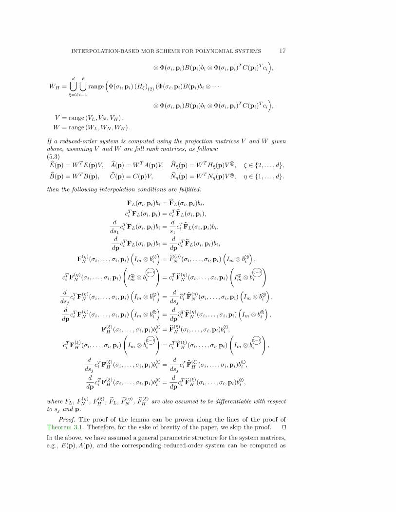
If a reduced-order system is computed using the projection matrices V and W givenabove, assuming V and W are full rank matrices, as follows:(5.3)

E(p) = WTE(p)V, A(p) = WTA(p)V, Hξ(p) = WTHξ(p)V ξ , ξ ∈ {2, . . . , d},

B(p) = WTB(p), C(p) = C(p)V, Nη(p) = WTNη(p)V η , η ∈ {1, . . . , d}.

then the following interpolation conditions are fulfilled:

FL(σi,pi)bi = FL(σi,pi)bi,

cTi FL(σi,pi) = cTi FL(σi,pi),

d

ds1cTi FL(σi,pi)bi =

d

s1cTi FL(σi,pi)bi,

d

dpcTi FL(σi,pi)bi =

d

dpcTi FL(σi,pi)bi,

F(η)N (σi, . . . , σi,pi)

(Im ⊗ b

η

i

)= F

(η)N (σi, . . . , σi,pi)

(Im ⊗ b

η

i

),

cTi F(η)N (σi, . . . , σi,pi)

(I 2

m ⊗ bη−1

i

)= cTi F

(η)N (σi, . . . , σi,pi)

(I 2

m ⊗ bη−1

i

)d

dsjcTi F

(η)N (σi, . . . , σi,pi)

(Im ⊗ b

η

i

)=

d

dsjcTi F

(η)N (σi, . . . , σi,pi)

(Im ⊗ b

η

i

),

d

dpcTi F

(η)N (σi, . . . , σi,pi)

(Im ⊗ b

η

i

)=

d

dpcTi F

(η)N (σi, . . . , σi,pi)

(Im ⊗ b

η

i

),

F(ξ)H (σi, . . . , σi,pi)b

ξ

i = F(ξ)H (σi, . . . , σi,pi)b

ξ

i ,

cTi F(ξ)H (σi, . . . , σi,pi)

(Im ⊗ b

ξ−1

i

)= cTi F

(ξ)H (σi, . . . , σi,pi)

(Im ⊗ b

ξ−1

i

),

d

dsjcTi F

(ξ)H (σi, . . . , σi,pi)b

ξ

i =d

dsjcTi F

(ξ)H (σi, . . . , σi,pi)b

ξ

i ,

d

dpcTi F

(ξ)H (σi, . . . , σi,pi)b

ξ

i =d

dpcTi F

(ξ)H (σi, . . . , σi,pi)b

ξ

i ,

where FL, F(η)N , F

(ξ)H , FL, F

(η)N , F

(ξ)H are also assumed to be differentiable with respect

to sj and p.

Proof. The proof of the lemma can be proven along the lines of the proof ofTheorem 3.1. Therefore, for the sake of brevity of the paper, we skip the proof.

In the above, we have assumed a general parametric structure for the system matrices,e.g., E(p), A(p), and the corresponding reduced-order system can be computed as


shown in (5.3). However, if we assume an affine parametric structure of the systemmatrices as follows:

(5.5)

E(p) =

te∑i=1

α(i)e (p)E(i), A(p) =

ta∑i=1

α(i)a (p)A(i), Hξ(p) =

thξ∑i=1

α(i)hξ

(p)H(i)ξ ,

B(p) =

tb∑i=1

α(i)b (p)B(i), C(p) =

tc∑i=1

α(i)c (p)C(i), Nη(p) =

tnη∑i=1

α(i)nη (p)N (i)

η ,

then the resulting reduced-order system can be determined, having the same structure

(5.6)

E(p) =

te∑i=1

α(i)e (p)E(i), A(p) =

ta∑i=1

α(i)a (p)A(i), Hξ(p) =

thxi∑i=1

α(i)hξ

(p)H(i)ξ ,

B(p) =

tb∑i=1

α(i)b (p)B(i), C(p) =

tc∑i=1

α(i)c (p)C(i), Nη(p) =

tnη∑i=1

α(i)nη (p)N (i)

η ,

where the original matrices are projected by the standard projection for given projec-tion matrices; for example:

(5.7)E(1) = WTE(1)V, A(1) = WTA(1)V, H

(1)ξ = WTH

(1)ξ V ξ , ξ ∈ {2, . . . , d},

B(1) = WTB(1), C(1) = C(1)V, N (1)η = WTN (1)

η V η , η ∈ {1, . . . , d}.

Furthermore, like in the non-parametric case, we can easily develop the connec-tion to the Loewner and shifted-Loewner type system, assuming we have sufficientinterpolation points for frequency and parameter variables. In Algorithm 5.1, we out-line all the steps to construct reduced-order systems for the parametric case, which isagain inspired by the Loewner-type MOR.

6. Numerical Results. In this section, we illustrate the efficiency of the pro-posed methods by means of two nonlinear PDE examples and their variants. All thesimulations were done on an Intel® Core™i7-6700 [email protected], 8 MB cache, 8GB RAM, Ubuntu 16.04, MATLAB Version 9.1.0.441655(R2016b) 64-bit(glnxa64).In the following, we note some details used in the numerical simulations:

• All original and reduced-order systems are integrated by the routine ode15s

in MATLAB with relative error and absolute error tolerances of 10−10.• We measure the output at 500 equidistant points within the time interval

[0, T ], where T is the end time.• We choose interpolation points for the frequency (s) in a logarithmic scale

for a given frequency range, and interpolation points for parameters (p) arechosen randomly using the rand command. To ensure reproducibility, we userandn(‘seed’,0) to initialize a random number generator.

6.1. Chafee-Infante equation. In our first example, we deal with a widely con-sidered one-dimensional Chafee-Infante equation. Its governing equation and bound-ary conditions are given as follows:

(6.1)v(t) = vxx + v(1− v2), x ∈ (0, L)× (0, T ), v(0, ·) = u(t), (0, T ),

vx(L, ·) = 0, (0, T ), v(x, 0) = 0, (0, L).

MOR of this example has been considered in various papers [8, 10, 11, 15], wherethe authors have proposed different methods to reduce it. The governing equation


Algorithm 5.1 Model Reduction for Parametric Polynomial Systems (1.1).

Input: The original system (1.1) with the affine structure as in (5.5), and aset of interpolation points for the frequency and parameters, i.e., σi and pi, i ∈{1, . . . , r}.Output: A reduced-order system given as in (5.6).

1: Determine V and W as shown in Theorem 5.1.2: Based on E(p) and A(p) in (5.5), define

L(i) = WTE(i)V, i ∈ {1, . . . , te}, L(i)s = WTA(i)V, i ∈ {1, . . . , ta}

[L(1), . . . ,L(te),L(1)

s , . . . ,L(ta)s

]= Y1Σ1X

T1(5.8)

L(1)

...L(te)

L(1)s

...

L(ta)s

= Y2Σ2X

T2 .(5.9)

3: Define Yr := Y1(:, 1 : r) and Xr := X2(:, 1 : r).4: Determine the compact projection matrices:

V := orth(V Xr) and W := orth(WYr).5: Determine a reduced-order system as shown in (5.6).

has cubic nonlinearity. In the literature, a common approach to reduce such a cubicnonlinear system via system-theoretic MOR is twofold. First, it is to rewrite thecubic system into a QB system by introducing auxiliary variables. Thereafter, onecan reduce it by employing a MOR scheme for QB systems such as balanced truncation[10], and interpolation based approaches, e.g., [2, 8, 11]. However, in this process, welose the original cubic nonlinearity structure in the reduced-order system. On theother hand, the proposed method, in this paper, allows us to reduce a cubic systemdirectly, having preserved the nonlinearity in the reduced-order system.

We set the domain length L = 1. The system of equations (6.1) is discretizedusing a finite-difference method by taking k = 500 grid points. Next, we aim atconstructing a reduced cubic system by applying Algorithm 3.1. For this purpose,we consider the frequency range

[10−3, 103

]. For comparison, we also rewrite the

cubic system into the QB form, which results in an equivalent QB system of ordernqb = 2 · 500 = 1000. We consider the same frequency range in order to employAlgorithm 3.1 to construct a reduced QB system.

First, in Figure 6.1, we observe the decay of the singular values, obtained fromthe Loewner pencil (L − sLs). As one can expect, the singular values related to theoriginal cubic system decay faster as compared to its equivalent QB form. Hence, forthe same order of the reduced-order system, we can anticipate a better quality reducedsystem. Next, we construct the reduced cubic and QB systems of order r = 10.To test the quality of both reduced cubic and QB systems, we perform time-domainsimulations using control inputs u(1)(t) = 10(sin(πt)+1) and u(2)(t) = 5 (te−t), which


Cubic system Quadratic-bilinear system

0 5 10 15 20 25 3010−20

10−10

100

Figure 6.1: Relative decay of singular values based on the Loewner pencils, obtainedusing the original cubic system and its equivalent transformed QB system.

Original system Cubic system Quadratic-bilinear system

0 1 2 3 40

0.5

1

1.5

2

Time

(a) Transient response.

0 1 2 3 410−9

10−5

10−1

Time

(b) Relative error.

Figure 6.2: Chafee-Infante equation: a comparison of the original and reduced-ordersystems for the input u(1) = 10 (sin(πt) + 1).

are compared in Figures 6.2 and 6.3 by showing the responses and relative errors. Ascan be seen from these figures, the cubic reduced-order system captures the dynamicsof the original system much better as compared to the QB system; precisely, we gainup to 3 orders of magnitude better accuracy using the new method.

6.2. The FitzHugh-Nagumo(FHN) model. As a second non-parametric ex-ample, we consider the FHN system, which describes basic neuronal dynamics. This isa coupled cubic nonlinear system, whose governing equations and boundary conditionsare as follows:

(6.2)εvt = ε2vxx + v(v − 0.1)(1− v)− w + q,

wt = hv − γw + q

with boundary conditions

v(x, 0) = 0, w(x, 0) = 0, x ∈ (0, L),

vx(0, t) = i0(t), vx(1, t) = 0, t ≥ 0,


Original system Cubic system Quadratic-bilinear system

0 1 2 3 4

0

0.5

1

Time


0 1 2 3 410−12

10−6

100

Time

(b) Relative error.

Figure 6.3: Chafee-Infante equation: a comparison of the original and reduced-ordersystems for the input u(2) = 5 (te−t).

Cubic sys. (two-sided) Cubic sys. (one-sided)

QB sys. (two-sided) QB sys. (one-sided)

0 10 20 30 40 5010−20

10−10

100

Figure 6.4: FHN model: relative decay of singular values based on the Loewnerpencils, obtained via one-sided and two-sided projection of the corresponding systems.

where h = 0.05, γ = 2, q = 0.05, L = 0.1 and i0 acts an actuating control input whichtakes the values 5 ·104t3e−t, and briefly mentioning, the variables v and w denote theactivation and de-activation of a neuron, respectively. We discretize the governingequation using a finite difference method, having taken 100 grid points. This leads toa cubic system of order n = 200. We use the same output setting as used, e.g., in [11].The system has two inputs and two outputs, thus, is a MIMO system. The MORproblem related to the FHN system has been considered by several researchers, see,e.g., [10, 11, 13]. Similar to the previous example, system-theoretic MOR of the FHNsystem has also been considered by first rewriting it into a QB system and employingMOR schemes such as interpolation-based and balanced truncation to reduce it. Thus,we obtain an equivalent QB system of order nqb = 300. However, by doing so, we losethe original nonlinear structure.

In order to apply Algorithm 3.1 to obtain reduced-order systems for the originalcubic and its equivalent QB systems, we choose 200 points in the frequency range[10−2, 102

]. In Figure 6.4, we first show the relative decay of the singular values

for the Loewner pencils (denoted by cubic sys. (two-sided) and QB sys. (two-sided)).


Therein, as expected, we observe that the singular values of the cubic system decayfaster as compared to its equivalent QB system. Next, we construct reduced cubicand QB systems of order r = 20. To determine the quality of the reduced systems,we perform time-domain simulations and plot the result in Figure 6.5. We observethat the obtained cubic reduced system captures the dynamics of the original systemvery well, whereas the reduced QB system is unstable. This illustrates a commonshortcoming of Algorithm 3.1 (the Loewner approach) that it does not always resultin a stable reduced system.

As a remedy, we propose to obtain a reduced-order system using Galerkin (one-sided) projection. For this, we determine the matrix V at Step 1 in Algorithm 3.1and set W = V . This is followed by determining Xr as shown in Step 4 of thealgorithm and determine the projection matrix Veff . Subsequently, we set Weff = Veff

and compute a reduced-order system. As a result, we have a reduced-order systemby Galerkin projection instead of Petrov-Galerkin projection. An advantage of doingGalerkin projection is the (local) stability of the reduced-order system in some cases.Next, we compute reduced systems of order r = 20 using the cubic and its equivalentQB form, using Galerkin projection.

First, we observe the decay of singular values in Figure 6.4, showing that forGalerkin projection as well, the decay is faster for cubic systems as compared tothe equivalent QB systems. Furthermore, we compare the transient response of thereduced-order systems obtained from Galerkin projection in Figure 6.5, which showsthat the cubic reduced-order system performs much better as compared to the QBreduced systems. Interestingly, we also observe that the reduced cubic systems, usingPetrov-Galerkin and Galerkin projection, tend to perform equally good as the timeprogresses but in the beginning, the reduced system, obtained using Petrov-Galerkinprojection, performs better.

Furthermore, we mention that the same order of accuracy as the reduced QBsystem (one-sided) of order r = 20 can be obtained from the reduced cubic orderr = 6 only. Surprisingly, we also observe that the typical limit-cycles behavior of thesystem can be captured by the reduced cubic system of order as low as r = 2. On theother hand, the reduced QB could not capture the typical limit cycles behavior belowthe order r = 15. This is a profound observation, which illustrates that keeping theoriginal structure of nonlinearity can lead to much better reduced-order systems.

6.3. Parametric Chafee-Infante equation. As our parametric example, weconsider the following parametric Chafee-Infante equation:

(6.3) v(t) = vxx + v(p− v2), x ∈ (0, L)× (0, T ),

where p ∈ [0.25, 2]. The boundary and initial conditions are the same as given in Sub-section 6.1, and the domain length and discretization scheme are also chosen the sameas in Subsection 6.1. Next, we aim at constructing a reduced cubic parametric systemusing Algorithm 5.1. For this, we take 200 points in the frequency range

[10−3, 103

]and the equal number of points for the parameter in the considered interval.

First, in Figure 6.6, we plot the decay of the singular values based on the Loewnerpencil, which decays exponentially. Subsequently, we determine a reduced parametricsystem of order r = 5. To compare the quality of the reduced-order system, wesimulate for the same inputs as used in Subsection 6.1 and for p = {0.25, 1, 2}. Weplot the transient response and relative errors in Figures 6.7 and 6.8, illustrating thatthe reduced parametric system can capture the dynamics of the system for differentinputs and different parameter.


Ori. sys. Cubic sys. (two-sided r = 20)

Cubic sys. (one-sided r = 20) QB sys. (one-sided r = 20)

Cubic sys. (two-sided r = 6)

0 5 10 15 20

0

0.5

1

Time


0 5 10 15 2010−12

10−6

100

Time

(b) Relative error.

Figure 6.5: FHN model: a comparison of the original and reduced cubic and QBsystems using one-sided and two-sided projections, having employed Algorithm 3.1.

0 5 10 15 20 25 3010−20

10−10

100

Rel

ati

vesi

ngu

lar

valu

es

Figure 6.6: Parametric Chafee-Infante equation: relative decay of singular valuesbased on the Loewner pencil.

6.4. Usage of CUR in ROM. In this section, we illustrate the usage of theCUR matrix approximation to further approximate the nonlinear reduced terms. Forthis, we again consider the Chafee-Infante equation as considered in Subsection 6.1.Using the same setting as shown in Subsection 6.1, we aim at determining reducedcubic systems using one-sided and two-sided projections. First, in Figure 6.9, we plotthe relative decay of the singular values based on the Loewner pencil, obtained usingthe one-sided and two-sided projection matrices. We observe that the singular valuesbased on the two-sided projection decay fast as compared to the one-sided projection.

Next, we construct reduced-order systems of order r = 10 using one-sided andtwo-sided projections using Algorithm 3.1, preserving the cubic nonlinear terms. Asdiscussed in Section 4, we can approximate these terms by making use of CUR matrixapproximation. For CUR matrix approximation, we choose 60 rows and 60 columnsof V (defined in (4.6)), which are chosen based on an adaptive sampling proposed in[29]. We would like to mention that the number 60 for row and columns is determinedbased on a trial and error method. An appropriate automatic method for CUR matrixapproximation, being suitable for MOR, needs further research. To this end, we have


Ori. sys. (p = 0.25) Ori. sys. (p = 1.0) Ori. sys. (p = 2.0)

Red. sys. (p = 0.25) Red. sys. (p = 1.0) Red. sys. (p = 2.0)

0 1 2 3 4

0

1

2

Time


0 1 2 3 410−10

10−7

10−4

Time

(b) Relative error.

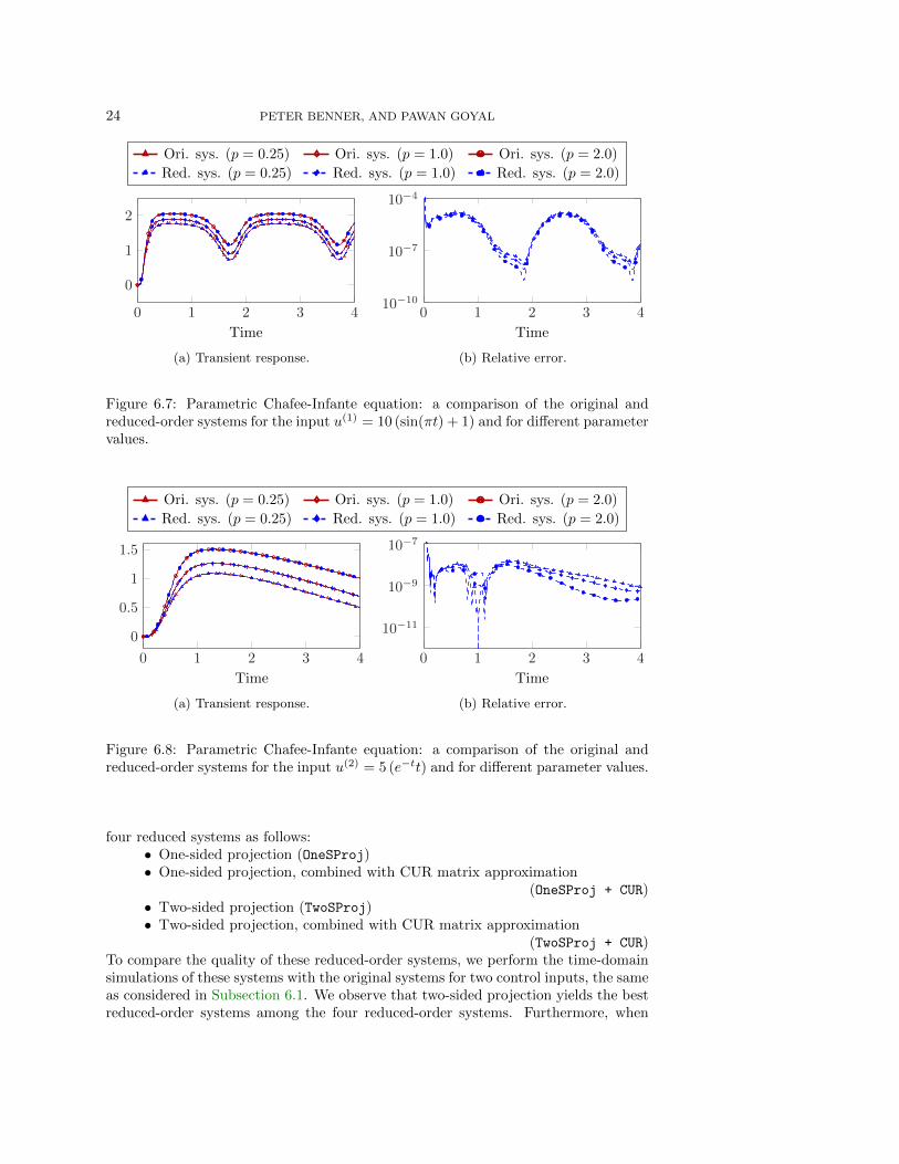
Figure 6.7: Parametric Chafee-Infante equation: a comparison of the original andreduced-order systems for the input u(1) = 10 (sin(πt) + 1) and for different parametervalues.

Ori. sys. (p = 0.25) Ori. sys. (p = 1.0) Ori. sys. (p = 2.0)

Red. sys. (p = 0.25) Red. sys. (p = 1.0) Red. sys. (p = 2.0)

0 1 2 3 4

0

0.5

1

1.5

Time


0 1 2 3 4

10−11

10−9

10−7

Time

(b) Relative error.

Figure 6.8: Parametric Chafee-Infante equation: a comparison of the original andreduced-order systems for the input u(2) = 5 (e−tt) and for different parameter values.

four reduced systems as follows:• One-sided projection (OneSProj)• One-sided projection, combined with CUR matrix approximation

(OneSProj + CUR)• Two-sided projection (TwoSProj)• Two-sided projection, combined with CUR matrix approximation

(TwoSProj + CUR)To compare the quality of these reduced-order systems, we perform the time-domainsimulations of these systems with the original systems for two control inputs, the sameas considered in Subsection 6.1. We observe that two-sided projection yields the bestreduced-order systems among the four reduced-order systems. Furthermore, when


Two-sided projection One-sided projection

0 10 20 30 40 5010−20

10−10

100

Figure 6.9: Chafee-Infante equation: relative decay of singular values using theLoewner pencil, obtained via one-sided and two-sided projections.

Ori. sys. TwosProj TwosProj + CUR

OneSProj OneSProj +CUR

0 1 2 3 4

0

1

2

Time


0 1 2 3 410−10

10−5

100

Time

(b) Relative error.

Figure 6.10: Chafee-Infante equation: a comparison of the original and (CUR com-bined) reduced-order systems for the input u(1) = 10 (sin(πt) + 1).

the two-sided reduced-order system is combined with CUR matrix approximation,then we notice that the quality of the reduced-order system decreases a little butstill provides a very good approximation of the original system. Interestingly, we alsonotice that CUR matrix approximation applied to the one-sided reduced-order systemalso performs really good, where the reduction in quality of OsP is very slim.

7. Conclusions. In this paper, we have discussed the construction of interpo-lating reduced-order systems for a parametric polynomial system. For this purpose,we have introduced generalized multi-variate transfer functions for the systems. Fur-thermore, we have proposed algorithms, inspired by the Loewner approach, to gener-ate good quality reduced-order systems in an automatic way. Furthermore, we havediscussed related computational issues and also the usage of the CUR matrix approx-imation in the simulations of reduced systems which may be helpful in some case. Wehave illustrated the efficiency of the approaches via several numerical experiments,where we have observed that preserving the original structure of the nonlinearity inreduced-order systems can lead to much better reduced-order systems.


Ori. sys. TwosProj TwosProj + CUR

OneSProj OneSProj +CUR

0 1 2 3 4

0

0.5

1

Time


0 1 2 3 410−15

10−7

101

Time

(b) Relative error.

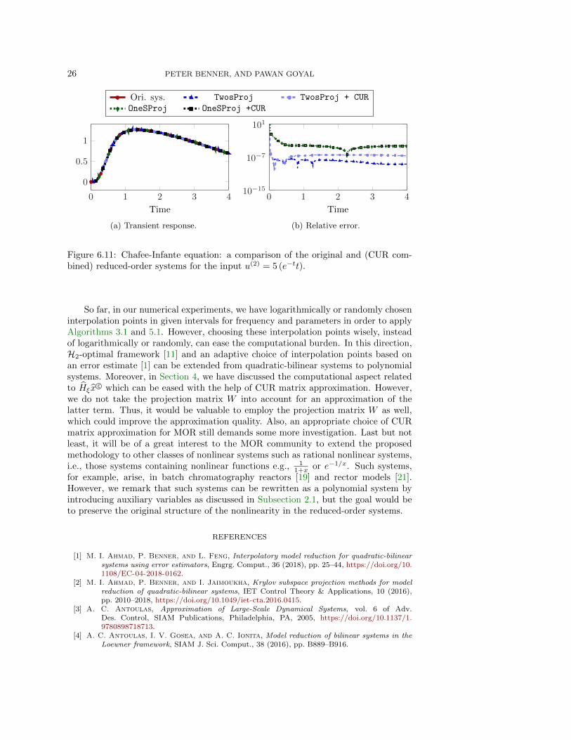
Figure 6.11: Chafee-Infante equation: a comparison of the original and (CUR com-bined) reduced-order systems for the input u(2) = 5 (e−tt).

So far, in our numerical experiments, we have logarithmically or randomly choseninterpolation points in given intervals for frequency and parameters in order to applyAlgorithms 3.1 and 5.1. However, choosing these interpolation points wisely, insteadof logarithmically or randomly, can ease the computational burden. In this direction,H2-optimal framework [11] and an adaptive choice of interpolation points based onan error estimate [1] can be extended from quadratic-bilinear systems to polynomialsystems. Moreover, in Section 4, we have discussed the computational aspect relatedto Hξx

ξ which can be eased with the help of CUR matrix approximation. However,we do not take the projection matrix W into account for an approximation of thelatter term. Thus, it would be valuable to employ the projection matrix W as well,which could improve the approximation quality. Also, an appropriate choice of CURmatrix approximation for MOR still demands some more investigation. Last but notleast, it will be of a great interest to the MOR community to extend the proposedmethodology to other classes of nonlinear systems such as rational nonlinear systems,i.e., those systems containing nonlinear functions e.g., 1

1+x or e−1/x. Such systems,for example, arise, in batch chromatography reactors [19] and rector models [21].However, we remark that such systems can be rewritten as a polynomial system byintroducing auxiliary variables as discussed in Subsection 2.1, but the goal would beto preserve the original structure of the nonlinearity in the reduced-order systems.

REFERENCES

[1] M. I. Ahmad, P. Benner, and L. Feng, Interpolatory model reduction for quadratic-bilinearsystems using error estimators, Engrg. Comput., 36 (2018), pp. 25–44, https://doi.org/10.1108/EC-04-2018-0162.

[2] M. I. Ahmad, P. Benner, and I. Jaimoukha, Krylov subspace projection methods for modelreduction of quadratic-bilinear systems, IET Control Theory & Applications, 10 (2016),pp. 2010–2018, https://doi.org/10.1049/iet-cta.2016.0415.

[3] A. C. Antoulas, Approximation of Large-Scale Dynamical Systems, vol. 6 of Adv.Des. Control, SIAM Publications, Philadelphia, PA, 2005, https://doi.org/10.1137/1.9780898718713.

[4] A. C. Antoulas, I. V. Gosea, and A. C. Ionita, Model reduction of bilinear systems in theLoewner framework, SIAM J. Sci. Comput., 38 (2016), pp. B889–B916.

https://doi.org/10.1108/EC-04-2018-0162

https://doi.org/10.1108/EC-04-2018-0162

https://doi.org/10.1049/iet-cta.2016.0415

https://doi.org/10.1137/1.9780898718713

https://doi.org/10.1137/1.9780898718713


[5] A. C. Antoulas, S. Lefteriu, and A. C. Ionita, A tutorial introduction to the Loewnerframework for model reduction, in Model Reduction and Approximation: Theory and Algo-rithms, P. Benner, A. Cohen, M. Ohlberger, and K. Willcox, eds., SIAM, 2017, pp. 335–376,https://doi.org/10.1137/1.9781611974829.ch8.

[6] M. Barrault, Y. Maday, N. C. Nguyen, and A. T. Patera, An ‘empirical interpolation’method: application to efficient reduced-basis discretization of partial differential equations,C. R. Math. Acad. Sci. Paris, 339 (2004), pp. 667–672.

[7] P. Benner and T. Breiten, Interpolation-based H2-model reduction of bilinear control sys-tems, SIAM J. Matrix Anal. Appl., 33 (2012), pp. 859–885.

[8] P. Benner and T. Breiten, Two-sided projection methods for nonlinear model order re-duction, SIAM J. Sci. Comput., 37 (2015), pp. B239–B260, https://doi.org/10.1137/14097255X.

[9] P. Benner, A. Cohen, M. Ohlberger, and K. Willcox, eds., Model Reduction and Approx-imation: Theory and Algorithms, Computational Science & Engineering, SIAM Publica-tions, Philadelphia, PA, 2017, https://doi.org/10.1137/1.9781611974829.

[10] P. Benner and P. Goyal, Balanced truncation model order reduction for quadratic-bilinearsystems, e-prints 1705.00160, arXiv, 2017, https://arxiv.org/abs/1705.00160.

[11] P. Benner, P. Goyal, and S. Gugercin, H2-quasi-optimal model order reduction forquadratic-bilinear control systems, SIAM J. Matrix Anal. Appl., 39 (2018), pp. 983–1032,https://doi.org/10.1137/16M1098280.

[12] P. Benner, V. Mehrmann, and D. C. Sorensen, Dimension Reduction of Large-Scale Sys-tems, vol. 45 of Lect. Notes Comput. Sci. Eng., Springer-Verlag, Berlin/Heidelberg, Ger-many, 2005.

[13] S. Chaturantabut and D. C. Sorensen, Nonlinear model reduction via discrete empiricalinterpolation, SIAM J. Sci. Comput., 32 (2010), pp. 2737–2764, https://doi.org/10.1137/090766498.

[14] K. Gallivan, A. Vandendorpe, and P. Van Dooren, Model reduction of MIMO systems viatangential interpolation, SIAM J. Matrix Anal. Appl., 26 (2004), pp. 328–349.

[15] I. V. Gosea and A. C. Antoulas, Data-driven model order reduction of quadratic-bilinearsystems, Numer. Lin. Alg. Appl., 25 (2018), p. e2200, https://doi.org/10.1002/nla.2200.

[16] C. Gu, QLMOR: A projection-based nonlinear model order reduction approach using quadratic-linear representation of nonlinear systems, IEEE Trans. Comput. Aided Des. Integr. Cir-cuits. Syst., 30 (2011), pp. 1307–1320, https://doi.org/10.1109/TCAD.2011.2142184.

[17] M. Gubisch and S. Volkwein, Proper orthogonal decomposition for linear-quadratic opti-mal control, in Model Reduction and Approximation: Theory and Algorithms, P. Ben-ner, A. Cohen, M. Ohlberger, and K. Willcox, eds., SIAM, 2017, pp. 3–63, https://doi.org/10.1137/1.9781611974829.ch1.

[18] S. Gugercin, A. C. Antoulas, and C. Beattie, H2 model reduction for large-scale lineardynamical systems, SIAM J. Matrix Anal. Appl., 30 (2008), pp. 609–638, https://doi.org/10.1137/060666123.

[19] G. Guiochon, A. Felinger, and D. G. Shirazi, Fundamentals of preparative and nonlinearchromatography, Academic Press, Boston, 2006.

[20] T. G. Kolda, Multilinear operators for higher-order decompositions, tech. report, Technicalreport SAND2006-2081, Sandia National Laboratories, Albuquerque, NM and Livermore,CA, 2006, https://www.sandia.gov/∼tgkolda/pubs/pubfiles/SAND2006-2081.pdf.

[21] B. Kramer and K. Willcox, Nonlinear model order reduction via lifting transformations andproper orthogonal decomposition, AIAA J., (2019), https://doi.org/10.2514/1.J057791.

[22] M. W. Mahoney and P. Drineas, CUR matrix decompositions for improved data analysis,Proc. of the National Academy of Sciences, (2009), pp. 697–702.

[23] A. J. Mayo and A. C. Antoulas, A framework for the solution of the generalized realizationproblem, Linear Algebra Appl., 425 (2007), pp. 634–662.

[24] G. P. McCormick, Computability of global solutions to factorable nonconvex programs:PartI–Convex underestimating problems, Mathematical programming, 10 (1976), pp. 147–175.

[25] A. Quarteroni, A. Manzoni, and F. Negri, Reduced Basis Methods for Partial DifferentialEquations, vol. 92 of La Matematica per il 3+2, Springer International Publishing, 2016.ISBN: 978-3-319-15430-5.

[26] A. C. Rodriguez, S. Gugercin, and J. Borggaard, Interpolatory model reduction of pa-rameterized bilinear dynamical systems, Adv. Comput. Math., 44 (2018), pp. 1887–1916,https://doi.org/10.1007/s10444-018-9611-y.

[27] W. J. Rugh, Nonlinear system theory, Johns Hopkins University Press Baltimore, 1981.[28] D. C. Sorensen and M. Embree, A DEIM induced CUR factorization, SIAM J. Sci. Comput.,

38 (2016), pp. A1454–A1482.

https://doi.org/10.1137/1.9781611974829.ch8

https://doi.org/10.1137/14097255X

https://doi.org/10.1137/14097255X

https://doi.org/10.1137/1.9781611974829

https://arxiv.org/abs/1705.00160

https://doi.org/10.1137/16M1098280

https://doi.org/10.1137/090766498

https://doi.org/10.1137/090766498

https://doi.org/10.1002/nla.2200

https://doi.org/10.1109/TCAD.2011.2142184

https://doi.org/10.1137/1.9781611974829.ch1

https://doi.org/10.1137/1.9781611974829.ch1

https://doi.org/10.1137/060666123

https://doi.org/10.1137/060666123

https://www.sandia.gov/~tgkolda/pubs/pubfiles/SAND2006-2081.pdf

https://doi.org/10.2514/1.J057791

https://doi.org/10.1007/s10444-018-9611-y


[29] S. Wang and Z. Zhang, Improving CUR matrix decomposition and the Nystrom approximationvia adaptive sampling, The Journal of Machine Learning Research, 14 (2013), pp. 2729–2769.

Documents

Interpolation-Based Model Order Reduction for Polynomial