International Diversification and the Home Bias Puzzle: The Role of Multinational Companies (MNCs)

Jenny Berrill1 and Colm Kearney2

AbstractBy investing in internationalised firms that are listed on the exchanges in their home countries, investors can reap the benefits of diversification without directly incurring the costs and risks associated with internationalisation at the level of the firm. The observed ‘home bias’ phenomenon can thus be consistent with optimal international diversification. To demonstrate this, we construct a firm-level sample of 1,289 firms from 7 countries, we classify their internationality from the geographical spread of their sales and subsidiaries, and we measure their performance using daily firm-level and market-level data from January 1999 to June 2007. Applying mean variance spanning and Sharpe ratio tests to determine and measure the statistical and economic significance of the diversification benefits of investing domestically in internationalised firms, we show that there are benefits to both domestic and international diversification and that the types of firm that provide these benefits varies across countries. Ccombining across all countries, we show that firms with global sales and subsidiaries provide the largest benefits to diversification. Overall, our work contributes to understanding the dimensions of, and resolving the ‘home bias’ puzzle.

KeywordsMNCs, international portfolio diversification, home bias, mean variance spanning.

JEL ClassificationF21, F23, G11

Contact Details1Institute for International Integration Studies, Trinity College, Dublin 2, Ireland. Tel: 353-1-896-3888. Fax: +353-1-896-3939, Email: berrilj@tcd.ie2School of Business Studies and Institute for International Integration Studies, Trinity College Dublin, Ireland. Tel: 353-1-8961774, Email: colm.kearney@tcd.ie, Homepage: www.internationalbusiness.ie.

1

1. Introduction

Enhanced integration throughout the world’s commodity, service and financial sectors

has created expanding opportunities for both firms and investors to reap the synergistic

gains from internationalisation. Firms have responded by internationalising their

activities across greater geographical and cultural distances through trading, forming

alliances, licensing, joint venturing and foreign direct investment (FDI). Given their

financial, knowledge and management resources, they choose the patterns of

internationalisation that maximize their risk-adjusted expected returns net of expected

costs (see Caves (1971) and Dunning (1980, 1988)). The extent to which firms create

value by successful internationalisation remains a controversial issue, with many studies

finding contradictory results (see Doukas and Lang (2003) for a review). Investors have

responded by holding greater proportions of more geographically and culturally distant

foreign assets in their portfolios. In a world with perfect markets, the international capital

asset pricing model (ICAPM) of Sharpe (1964) and Linter (1965) predicts that investors

will hold the world market portfolio. Interestingly, however, the extent to which investors

diversify internationally remains significantly less than many financial analysts and

researchers believe should be observable. This is the so-called ‘international

diversification puzzle’, also called the ‘home-bias puzzle’. It arises because although the

benefits of international portfolio diversification are significantly positive, and although

the costs and risks associated with achieving them appear small relative to those

associated with internationalising at the level of the firm, investors continue to hold the

majority of their financial portfolios in domestic rather than international assets.

The observed home bias of portfolio investors appears to be inefficient, but the literature

offers a variety of explanations for the phenomenon including transaction costs, taxes,

information asymmetries, currency risk, legal restrictions, political risk and other

controls. For example, French and Poterba (1991) show that investors in Japan and the

United States exhibit home bias by expecting domestic returns to exceed those on a

diversified portfolio. Tesar and Werner (1995) show that geographical proximity,

language compatibility and trade links are more important than correlation structures for

international portfolio investors. Baxter and Jermann (1997) attribute home bias to

2

investors hedging the risks associated with their non-traded human capital. Coval and

Moskowitz (1999) demonstrate ‘local bias’ amongst United States investment managers.

Hasan and Simaan (2000) and Ahearne, Griever and Warnock (2004) show how home

bias results from poor or costly information and/or information asymmetries. Overall, it

is widely agreed that home bias continues to exist despite the benefits of international

diversification, and that it results from investor preferences at least as much as from

market imperfections (see inter alia, French and Poterba (1991), Cooper and Kaplanis

(1994) and Tesar and Werner (1995), Portes and Rey (1998, 2005), Wei (2000), Portes,

Rey et al (2001), Karolyi and Stulz (2002), Guerin (2006), and Rosati and Secola

(2006)).

In this paper, we consider an alternative explanation of the observed home bias puzzle.

Combining the resources of Datastream, Worldscope and Dunn and Bradstreet’s Who

Owns Whom, we construct a sample of 1,289 firms from Britain, Canada, France,

Germany, Italy, Japan and the United States. Our sample comprises all firms listed on

the countries’ exchanges (the FTSE 100, the TSX 60, the SBF 120, the HDAX 110, the

MIB-SGI 174, the Nikkei 225 and the S&P 500) for which we have the full set of data.

We provide a detailed classification of the multinationality of these firms’ operations

from the geographical spread of their sales and their subsidiaries, and we measure their

performance using 2,217 observations of daily firm-level and market-level data from 1

January 1999 to 30 June 2007. Using this multi-country, firm-level dataset with almost 3

million observations, we examine the extent to which investors can gain international

diversification without having to invest in foreign markets. By investing in

internationalised firms that are listed on the exchanges in their home countries, investors

may be able to ‘free ride’ the costs and risks associated with internationalisation at the

level of the firm by reaping the benefits directly from internationalised firms. Both

Dahlquist and Robertson (2001) and Cai and Warnock (2004) show that investors tend to

favour large internationalised firms. The literature on whether investing in multinational

companies (MNCs) yields investors the benefits of international portfolio diversification,

however, produces mixed results. We show that these conflicting results are due to

inconsistencies in how researchers have classified MNCs in their empirical studies.

3

Building on Aggarwal, Berrill and Kearney (2007), we provide a robust classification of

the firms in our sample that allows us to examine how domestic investors can reap the

benefits of international diversification in a manner that is consistent with the observed

home bias phenomenon being part of an optimal investment strategy.

Our paper has a number of novel features. First, our classification of the degree of

multinationality of MNCs allows us to provide a deeper analysis than has appeared in the

literature to date of the types of firm that provide diversification benefits to investors.

Classifying the firms in our sample as ‘domestic’, ‘regional’, ‘trans-regional’ or ‘global’,

we construct investment portfolios from the firm-level characteristics that allow us to

examine the benefits of diversification at various degrees of internationality. Second,

existing studies of the diversification benefits of investing in MNCs (such as Huberman

and Kandel (1987), Bekaert and Urias (1996) and Errunza, Hogan and Hull (1999))

typically examine the question from a United States perspective. The United States has

one of the most diversified economies and one of the most developed stock markets in

the world, and is unlikely to yield results that apply to representative investors in other

countries. Following Rowland and Tesar (2004) who take the viewpoint of investors in

each of the G7 countries, we also apply our methodology to the perspective of investors

in each country. Third, using mean variance spanning tests to calculate the statistical

significance of differences in portfolio performance, and using changes in Sharpe ratios

to measure the economic significance of such differences, we examine the diversification

benefits to investing in various types of MNC, considering in turn the case of frictionless

markets in which investors can short sell assets without costs, and the case where there

are short selling constraints. Although it is likely that short selling restrictions are

relevant in this context, previous studies have not considered how the introduction of

short selling constraints affects their results. Finally, unlike previous studies that have

focussed exclusively on the advantages of international diversification by using some

market index or a sample of arbitrarily defined domestic firms to represent the domestic

market, our approach allows us to establish and test a richer set of hypotheses about the

extent to which the benefits of diversification are consistent across countries at the

‘regional’, ‘trans-regional’ and ‘global’ levels of internationality, and whether investors

4

in one country can obtain better diversification benefits by investing in ‘domestic’ of

international firms in other countries.

Amongst our main findings are the following. First, domestic diversification has benefits

that have been neglected heretofore in the home bias literature. In Britain, France and

Germany, for example, domestically quoted firms have lower correlations with each

other than the domestic market index has with foreign market indices. Our results from

174 mean variance spanning tests on domestic diversification fail to reject spanning in

only 7 of these tests, confirming the existence of domestic diversification benefits in

almost all cases. Second, when we classify all firms on a scale of ‘domestic’, ‘regional’,

‘trans-regional’ and ‘global’, the types of firms that provide diversification benefits vary

across countries. Third, when we combine each category of firm across all countries,

however, we find that firms with global sales and global subsidiaries provide the largest

benefits to diversification. This finding is both intuitive and robust, and it demonstrates

that when the empirical analysis is done methodically in a way that recognises

differences in multinationality across firms and countries, investors can indeed exhibit

home bias while reaping the benefits from international diversification.

The remainder of our paper is structured as follows. In section 2, we describe our dataset

and outline our taxonomy for classifying the degree of internationalisation of the firms in

our sample. In section 3, we present our hypotheses and describe our testing

methodology. Our results are presented in section 4. In section 5, we provide a set of

robustness tests. In section 6, we summarise our argument and draw our conclusions.

2. Data and taxonomy

2.1 Data sample

We commenced our sample construction by identifying 1,289 firms listed on the

following exchanges in Britain, Canada, France, Germany, Italy, Japan and the United

States: the FTSE 100, the TSX 60, the SBF 120, the HDAX 110, the MIB-SGI 174, the

Nikkei 225 and the S&P 500. This contains all firms for which we have the full set of

data. We provide a detailed classification of the multinationality of these firms’

5

operations from the geographical spread of their sales and their subsidiaries, and we

measure their performance using 2,217 observations of daily firm-level and market-level

data from 1 January 1999 to 30 June 2007. Using this multi-country, firm-level dataset

with almost 3 million observations, comprising 15,512 market level observations and

2,856,424 firm level observations, we classify each firm’s degree of internationalisation

from the geographical spread of its sales and subsidiaries. We obtain the geographical

breakdown of firm-level sales from the Worldscope databank. This data is taken from

company accounts for the year end 31 December 2005 or as close to this date as possible.

A geographical breakdown of each firm’s subsidiaries is obtained from ‘Who Owns

Whom’ 2005/06 by Dunn and Bradstreet Ltd. This publication lists parents and

subsidiaries of firms, with the country of each subsidiary1. We use 4 categories of

multinationality – domestic, regional, trans-regional and global – for both sales and

subsidiaries. This leads to the creation of up to 8 categories of firm within each country.

We use our sales and subsidiary categorisations to create market capitalisation weighted

indices of firms in each category. We calculate market capitalisation indices using a

similar methodology to that of the S&P 500 and the FTSE 1002. We generate 24 sales

indices and 27 subsidiary indices (Canada and Japan do not have firms with global sales,

Japan and Germany do not have firms with regional sales and Canada has no firms with

regional subsidiaries). This leads to a total of 51 indices with 113,016 daily observations.

We use daily exchange rate data from Datastream to convert each of our 51 indices into

each of the 5 currencies of the G7 countries – a total of 255 indices and 565,080 daily

observations. We also convert each of our 7 market indices into each of the 5 currencies

of the G7 countries – a further 35 indices with 77,560 daily observations.

We next create aggregate market value weighted indices of all domestic, all regional, all

trans-regional and all global firms (from all of the G7 countries combined together). We

analyse the sales and subsidiary indices separately. We create 8 aggregate indices in each

currency with 17,728 daily observations. Each of these indices is converted into each of

the 5 currencies within our dataset leading to a total of 40 indices with 88,640 daily

observations. Any firm with missing market value data is excluded from the index

calculation. We use 3-month Treasury Bill rates as the risk free rate in each country3.

6

2.2 Taxonomy of internationaslisation

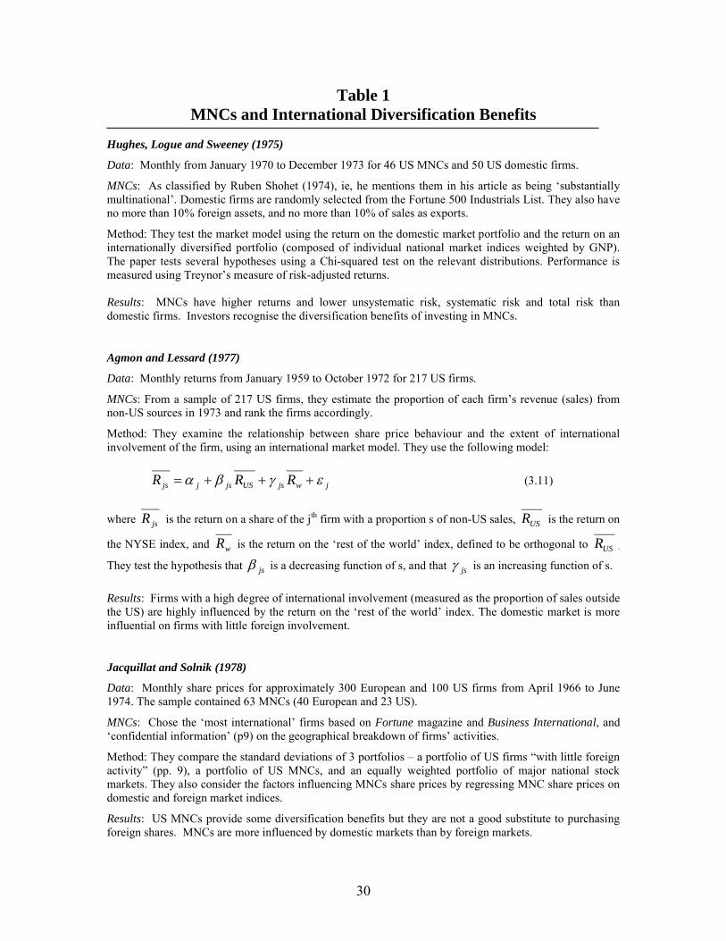
Previous research on whether internationalised firms provide the benefits to international

portfolio diversification produces mixed results. Table 1 contains the details. Hughes,

Logue and Sweeney (1975), Agmon and Lessard (1977), Mikhail and Shawky (1979),

Logue (1982), Errunza, Hogan and Hull (1999) and Cai and Warnock (2004) all conclude

that investing in MNCs can yield international diversification benefits to domestic

investors. By way of contrast, however, Jacquillat and Solnik (1978), Senchack and

Beedles (1980), Brewer (1981), Fatemi (1984), Michel and Shaked (1986), Mathur,

Singh and Gleason (2001), Salehizadeh (2003) and Rowland and Tesar (2004) all

conclude the opposite. These conflicting results are due to inconsistencies in how

researchers have classified MNCs in their empirical studies. Researchers have adopted

pragmatic approaches to creating their MNC samples, and they have operationally

defined international firms on the basis of characteristics such as the level (or percentage

relative to total) of foreign assets, foreign investments and foreign sales, to name a few.

Three examples of this approach are as follows. Michel and Shaked (1986) examine

Fortune 500 firms in the manufacturing sector. They classify firms as MNCs if at least

20 percent of their total sales are foreign and if they have direct capital investment in at

least 6 foreign countries, and as domestic if they have less than 10 percent of their sales,

profits and assets abroad. A firm with 20 percent foreign sales to one country would

therefore be grouped alongside another firm with 60 percent foreign sales to three

countries, and a third firm with 15 percent foreign sales spread over six countries

worldwide would not feature as either multinational or domestic, and if its percentage of

foreign sales declined to 9 percent while still being in 6 countries worldwide, it would be

classified as domestic. Errunza, Hogan and Hung (1999) use a sample of 30 of the 50

largest United States companies in the world ranked by the Fortune 100 list.4 Because

their sample is based on total sales without any consideration of whether they are foreign

or domestic, their sample potentially contains firms that are domestic, global, or some

combination in between. Rowland and Tesar (2004) classify firms as domestic or

multinational based on the listing of firms in the Worldwide Branch Locations of

7

Multinational Companies (Hoopes 1994). Firms included in this list have at least one

branch, subsidiary or other holding abroad, with the number of branches ranging from 2

to 500. This classification is also too broad because firms with very different levels of

international diversification are grouped together.5 Their conclusion from 411 firms in 7

countries that MNCs offer little diversification benefits is intuitive if most of these firms

have few foreign branches, but is questionable if the firms have many foreign branches

worldwide.

In order to overcome this ambiguity, we classify firms using the taxonomy of Aggarwal,

Berrill and Kearney (2007) which defines the degree of internatinalisation of a firm along

two dimensions: breadth and depth. To implement the breadth dimension of

multinationality, we divide the world into 6 regions, based on the inhabited continents:

Africa, Asia, Europe, North America, Oceania and South America. We measure the

breadth of multinationality as the extent of geographical spread across the world using 4

categories: domestic, regional, trans-regional and global. An activity associated with a

corporation that takes place entirely within the home country is referred to as domestic

(D). An activity that takes place within the region in which the firm is headquartered is

referred to as regional (R). We further delineate R into 3 categories, R1 (less than one-

third of the countries in a region), R2 (between one-third and two-thirds of the countries

in a region) and R3 (more than two-thirds of the countries in a region). An activity

associated with a firm that takes place in more than one region (but not fully global) is

defined as trans-regional (T), and this category is further subdivided into T2 (two

regions), T3 (three regions), T4 (four regions) and T5 (five regions). Finally, an activity

that takes place in all six regions of the world is classified as ‘global’ (G). To implement

the depth dimension of multinationality, we use two categories: trading and investments.

Trading involves sales and purchases made by the firm. Investments, such as joint

ventures and subsidiaries, entail a deep engagement with foreign markets and a high

exposure to other countries’ business, economic and political risks. We combine the

breadth and depth dimensions of the degree of internationalisation to form a matrix of

multinationality. We first simplify the breadth measure by combining the three ‘within-

region’ decompositions (R1, R2 and R3) and the 4 trans-regional groups (T2, T3, T4 and

8

T5) to reduce the breadth categories from 9 to 4; D, R, T and G. This results in the 2 x 4

matrix shown below.

Breadth of Geographical Spread

Depth of Engagement

Domestic Regional Trans-regional

Global

Trading TD TR TT TG

Investments ID IR IT IG

This 2 x 4 matrix allows us to classify 16 different types of firm in terms of their

multinationality, ranging from purely domestic firms (TD-ID) that carry out all their

trading activities and investments entirely within their home countries, to deeply global

MNCs (TG-IG) that have trading activities and subsidiaries in all regions of the world. In

between these cases, there are 14 different degrees of multinationality. These are

presented in Table 2, which describes eight types of regional and trans-regional firms

(numbered 2 to 9) and seven types of global corporation (numbered 10 to 16).

Looking first at the eight regional and trans-regional firms numbered 2 to 9 in Table 2 we

can differentiate between firms that have increasingly broad but shallow patterns of

internationalisation (firms 2 – 3), and those that are more deeply engaged with foreign

markets (firms 4 – 9). One would not expect a type 4 firm (TD-IR) with domestic trading

and regional investments to deliver the same international diversification benefits as a

type 9 firm (TT-IT) with trans-regional sales and subsidiaries. But this is precisely what

many researchers assume when they combine these firms in their data sets - along with

purely domestic firms (TD-ID) and deeply global MNCs (TG-IG)! Looking next at the

seven global MNCs numbered 10 to 16 in Table 2, they can be global in their trading

(firms 10 – 12), their investments (firms 13 – 15), or both (firm 16). Firm 10 (TG-ID) is

shallowly global and deeply domestic, whereas firm 12 (TG-IT) is shallowly global and

deeply trans-regional.

Table 3 shows the number of firms from each market index falling into each category.

The percentage of firms with purely domestic sales ranges from 5 percent of German

9

firms to 30 percent of Italian firms. In the US, 29 percent of firms are classified as

domestic in their sales. These market indices are commonly used in empirical analysis to

represent domestic firms and the domestic economy. The average amount of firms

classified as domestic in their sales is 20 percent. These data suggest that while market

indices are a good measure of the domestic stock market, they may not be a good

measure of the domestic economy and economic activity within the domestic market.

They also show that each market index differs in how appropriately it represents

domestic factors. At the other end of the spectrum, the percentage of global firms ranges

from 8 percent for the UK to zero for Canada and Japan. In all countries, the majority of

firms are classified as trans-regional – on average 73 percent of firms across the 7 indices

are classified as trans-regional in their sales. These data demonstrate that domestic

market indices and domestically quoted firms are exposed to international influences.

We calculate the correlation coefficient (in each domestic currency) between each market

index and the other 6 markets and get the average of these figures. These correlations are

detailed in Table 4. The average correlation between the Nikkei 225 and the other 6

market indices is 0.2019. The average correlations with the foreign market indices in our

sample for the other market indices are as follows: Nikkei 225 (0.2019), S&P 500

(0.3468), TSX 60 (0.3621), MIB Storcio General (0.5043), FTSE 100 (0.5355), HDAX

110 (0.5833) and SBF 120 (0.608). The Nikkei index is the least correlated with the

other indices suggesting that Japanese investors benefit most from diversification within

the G7 countries. European investors benefit least from international diversification

within the G7 countries. The individual correlations in Table 4 suggest that geographical

proximity has a strong influence on the relationship between markets. The US and

Canada have the highest correlations with each other while European markets are also

highly correlated with each other. Japan has the lowest correlation with each of the other

countries, apart from Italy, which is least correlated with the US market. Table 4 also

details the correlations between each category of firm (domestic, regional, trans-regional

and global) and each foreign market index. We show the average correlation of each

category of firm with the 6 foreign indices in the sample. The trans-regional firms in all

countries are the most highly correlated with the foreign market indices. Domestic firms

10

are the least correlated with foreign market indices in all countries with the exception of

the US and Italy. Italy provides an unusual case in that global firms are the least

correlated with foreign market indices.

3 Hypotheses and testing methodology

Several methods have been used to assess how useful MNCs are in providing the benefits

to international diversification. These include using the international market model to

investigate the influence of domestic and foreign market indices on individual shares,

comparing the risk adjusted performance of MNCs and domestic firms, comparing firms

on the basis of returns, standard deviations, betas, coefficients of variation, the Sharpe,

Treynor and Jensen measures, and more recently, mean variance spanning tests. We first

analyse both the statistical and economic significance of the diversification benefits. We

use mean variance spanning tests to calculate the statistical significance. In doing this,

we use the regression tests for mean variance spanning developed by Huberman and

Kandel (1987) and De Roon and Nijman (2001).

To construct the mean variance spanning tests, we follow Huberman and Kandel (1987)

and Kan and Zhou (2001) by considering a set of K benchmark assets and N test assets.

The question is, whether conditional on the K benchmark assets, the addition of the N test

assets can shift the mean variance efficient frontier. Alternatively, conditional on the

K+N benchmark and test assets, can the subset of K benchmark assets yield the same

diversification benefits. In common parlance, we are interested in whether the K

benchmark assets span the extended set of K+N assets. To set up the test, we begin by

defining t,1R as the K×1 vector of either raw or excess returns on the K benchmark

assets at time t, we define t,2R as the N×1 returns on the N test assets at time t, and we

combine t,1R and t,2R in the K+N vector ''t,2

't,1t ]R,R[R = . The expected returns

]R[E t and the variances ]R[Var t on these K+N assets can be written as

2

1t μ

μμ]R[E ==

2221

1211t VV

VVV]R[Var == (1)

11

The mean variance spanning test proceeds by estimating the following model, which

regresses the N test asset returns on the K benchmark asset returns,

tt,1t,2 εRβαR ++= (2)

with tε ~ )Σ,0(N , 2,t 1,t 2 1α E[R ] βE[R ] μ βμ= - = - , and 121 11β V V -= .

By defining N Kδ 1 β1= - , we can see that in order to test whether the set of K

benchmark assets spans the broader set of K+N assets amounts to testing the joint

hypothesis that Nα δ 0= = . If this hypothesis is upheld, it implies that for every test

asset, we can obtain a portfolio of the K benchmark assets that has the same expected

return (because Nα 0= and K Nβ1 1= ) and a lower variance (because t,1R and tε are

uncorrelated while tVar(ε ) is positive definite.

To derive the form of the mean variance spanning test that we use in the next section, we

rewrite equation (2) in matrix notation as

R Xβ Σ= + (3)

with the unconstrained maximum likelihood estimates of β and Σ being determined as

usual by

^

1 'β (X ' X ) (X R)-= and ^ ^ ^1Σ (R X β)'(R X β)

T= - -

To derive the tests of spanning and to facilitate their geometric presentation, letting

^ T

tt 1μ Σ R / T

== and

^ T ^ ^

t tT 1V Σ (R μ)(R μ)'

== - - , we define three constants, α , b , c

and d that are important determinants of the location and shape of the efficient frontier.

We do this for the efficient frontiers with K and with K+N assets. For K assets, we have

12

1^ ^ ^ ^

K K 11 Ka μ ' V μ-

= , 1^ ^ ^

K K 11 Kb μ ' V 1-

= , 1^ ^ ^

K K 11 Kc 1' V 1-

= and 2^ ^ ^ ^

K K K Kd a c b= - .

The equivalent for K+N assets is 1^ ^ ^ ^

K N K N K Na μ ' V μ-

+ + += , 1^ ^ ^

K N K N K Nb μ 'V 1-

+ + += ,

1^ ^ ^

K N K N K Nc 1' V 1-

+ + += , and 2^ ^ ^ ^

K N K N K N K Nd a c b+ + + += - . As we move from the

frontier with K benchmark assets to the more general frontier with K+N assets, these

constants will change by ^ ^ ^

K N KΔa a a+= - , ^ ^ ^

K N KΔb b b+= - and ^ ^ ^

K N KΔc c c+= - .

This allows us to write the following two matrices, the latter of which is termed the

marginal information matrix (see Jobson and Korkie (1989)).

^ ^^

K K^ ^

K K

1 a bG

b c

+= and

^ ^^

^ ^

Δa ΔbH

Δb Δc= (4)

Combining the ^

G and ^

H matrices in (4), recalling that ^

Σ denotes the unconstrained

(with K+N assets) maximum likelihood estimate of Σ in (3), denoting the constrained

(with K assets) maximum likelihood estimate of Σ in (3) as ~

Σ , and letting ~^

1U Σ Σ-= ,

the likelihood ratio test of whether the K benchmark assets span the K+N benchmark

and test assets is:

LR T ln(U)= - (5)

where

~^1U Σ Σ-= =

^

^ ^

G

G H+ =

^^ ^2

K K K^^ ^2

K N K N K N

(1 a )c b

(1 a )c b+ + +

+ -

+ -

13

=

NK

NK

K

K

NK

K

c

d1

c

d1

c

c

Huberman and Kendel (1987) and Jobson and Korkie (1989) show that the distribution of

the likelihood ratio test under the null is distributed as

1UN

NKTF 2

1

1

c

d1

c

d1

c

c

N

NKT

K

K

NK

NK

K

NK (6)

We know that the standard deviations of the minimum variance portfolios of the K

benchmark assets and the K+N benchmark and test assets are ^

Kc/1 and ^

NKc/1 + ,

so the first ratio on the right hand side of (6) is their ratio which is always greater than

one. Kan and Zhou (2001) also show that the second ratio is the length of the asymptote

from to the K+N efficient frontier benchmark divided by its equivalent to the restricted

frontier of the K benchmark assets, and this ratio is also greater than one.

Diagrammatically, Kan and Zhou (2001) show that the likelihood ratio test, the Wald test

and the Lagrange multiplier test are closely related tests of mean variance spanning as

shown in Figure 1.

In our tests, we focus on the Wald test for the case of N = 1. Kan and Zhou (2001) show

that although the power of the three spanning tests is difficult to gauge when N > 1, the

likelihood ratio test is generally not the most powerful. They also show that for the case

of N = 1, differences in the minimum variance portfolio are more important that

14

differences in the tangent portfolio, and the Wald test is the most powerful of the three.

We estimate equation (1) using OLS and the 2n restrictions in equation (2) are tested

using a Wald test. The distribution of the asymptotic Wald test statistic of the null

hypothesis is:

2221 ~ nTW (7)

Kan and Zhou (2001) outline a procedure whereby mean-variance spanning tests can be

decomposed into two parts: the spanning of the global minimum-variance portfolio and

the spanning of the tangency portfolio. In this case, we can re-write the Wald test statistic

as:

1

ˆ1

ˆ11

ˆ

ˆ2

1

2

12

2

1

1

GMVR

GMVR

R

R

R

RTTW

(8)

where (σˆR1)2 and (σˆR)2 are the global minimum-variance of the benchmark assets and

benchmark plus the extended assets respectively. θˆR1(R1GMV) is the slope of the

asymptote of the mean-variance frontier for the benchmark assets, and θˆR(R1GMV) is the

slope of the tangency line of the mean-variance frontier for the benchmark portfolio plus

the extended set (based on the return of global minimum-variance portfolio for the

benchmark assets, R1GMV). The first term measures the change of the global minimum-

variance portfolios due to the addition of the new asset. The second term measures

whether there is an improvement of the squared tangency slope when the extended set of

assets is added to the benchmark asset.

Kan and Zhou (2001) show that the asymptotic tests have very good power for test assets

that can reduce the variance of the global minimum-variance portfolio, but have little

power against test assets that can only improve the tangency portfolio. They therefore

suggest a step-down procedure, whereby they first test α = 0n and then test δ = 0n

conditional on α = 0n. The step-down asymptotic Wald tests can then be written as:

15

2

42

231

~

,~

n

n

TW

TW

(9)

If we reject the hypothesis due to the first test, the tangency portfolios are very different.

If we reject due to the second test, the global minimum-variance portfolios are very

different.

The OLS tests above assume the error terms are normally distributed and homoskedastic.

In order to test the robustness of this assumption, we also perform all tests using the

Generalised Method of Moments (GMM) approach. The GMM approach has the

advantage that it does not require information on the exact distribution of the error terms.

We use the following GMM Wald test:

22

'1''' ~ˆˆNNTTNTa vecIASIAvecTW

(10)

where the moment condition is

'

10 knt EXEgE (11)

ttT ggES ' (12)

111

'1

111

'11

ˆ1ˆ

ˆˆˆ1

Vb

VaA

k

T

(13)

We also conduct step-down GMM Wald tests to disentangle the two sources of spanning.

The step-down GMM Wald test statistics are distributed as chi-square with N degrees of

freedom.

The null hypothesis is that the mean variance portfolio frontiers coincide at all points. If

the null hypothesis of spanning is rejected, however, this does not provide information

about the magnitude of the shift in the efficiency frontier. We measure the economic

significance of the diversification benefits using changes in the Sharpe (1966) ratio of the

16

optimal portfolios. We calculate the Sharpe ratio for the mean-variance efficient portfolio

based on the k benchmark assets (and a risk-free asset) and the Sharpe ratio for the mean

variance efficient portfolio based on all K + N assets (and a risk free asset), both in the

case of frictionless markets and in the case of short selling constraints. As shown by

Tobin (1958), the composition of the tangency portfolio is independent of investors’

preference structure. A difference between the Sharpe ratios of the benchmark and

extended set assets indicates that investors can increase their risk-return trade off by

investing in the N additional assets. If there is spanning, then there is no improvement in

the Sharpe ratio possible by including the additional assets in the portfolio.

4. Hypotheses and results

We empirically test 4 hypotheses in relation to obtaining the benefits from international

portfolio diversification. We test each hypothesis from the point of view of investors in

each of the G7 countries. We begin by using market level data to test if the benefits from

international portfolio diversification exist for investors within the G7 countries. We use

mean variance spanning tests to investigate if benefits exist and changes in the Sharpe

ratios of the optimal portfolios as a measure of these benefits. Specifically, hypothesis 1

may be stated as follows:

Hypothesis 1

H0: There are no benefits to international portfolio diversification.

H1: There are benefits to international portfolio diversification.

We use the domestic market index as the benchmark portfolio and individual

international market indices as the extended sets. We test this hypothesis with 42 (7 x 6)

tests of whether each country’s market index spans each of the other country’s market

indices, all converted to the home country’s currency. We reject the hypothesis of

spanning in all 42 tests with one exception. In the UK, we fail to reject the hypothesis

that the HDAX spans the FTSE index. These results show that the benefits from

international portfolio diversification exist for investors within the G7 countries. The

OLS step down results reveal that in all tests where we reject spanning, we reject because

17

the global minimum variance portfolios (rather than the tangency portfolios) differ

significantly from each other. In Japan and the US, the rejection of the hypothesis that the

TSX spans the domestic index is also due to the tangency portfolios differing from each

other. In all other tests, however, rejection is not due to differences in the tangency

portfolios. This implies that, in most cases, the greatest benefits are achieved at lower

levels of risk. The GMM analysis confirms these results with two exceptions: we fail to

reject the hypothesis that the HDAX spans the SBF in France and that the SBF spans the

MIB in Italy. Table 5 details the increases in the Sharpe ratios of the optimal (tangency)

portfolios when additional market indices are added to the domestic market index. The

Sharpe ratio tests show that in all countries except Canada, the TSX provides the greatest

benefits. The HDAX and SBF are strong performers in all markets, with the exception of

Canada. In Japan, the US and the UK, the 4 best performing indices are the TSX, SBF,

HDAX and MIB indices. In summary, we find support for the alternative hypothesis that

there are benefits to international portfolio diversification within the G7 countries.

The home bias literature demonstrates that, although there are benefits to international

portfolio diversification, investors continue to hold the majority of their financial

portfolios in domestic rather than international assets. Previous studies tend to focus

exclusively on the advantages of international diversification and do not investigate the

diversification benefits from investing in domestic markets. We investigate these benefits

as an alternative explanation to the ‘home bias puzzle’. If investors can use domestically

quoted firms to gain exposure to international influences, a home biased attitude to

international investing may be justified. This leads to our second hypothesis, which may

be stated as follows:

Hypothesis 2

H0: There are no benefits to international diversification by investing domestically.

H1: There are benefits to international diversification by investing domestically.

We run up to 7 tests on the benefits of investing in domestically quoted firms in each

country. We use our index of domestic firms as the benchmark set and perform tests

using regional, trans-regional, global, and various combinations of these firms as the

18

extended sets. We reject spanning in 32 out of a total of 35 tests, demonstrating that there

are benefits to international portfolio diversification by investing domestically. We fail to

reject spanning in 3 tests in the US market. We fail to reject spanning in tests where

domestic firms are used as the benchmark set and regional firms, global firms and a

portfolio of regional and global firms are the extended sets. The step down Wald tests

show that we fail to reject spanning at both the tangency and the minimum variance

points in these 3 cases. In cases where we reject spanning, we reject because the global

minimum variance portfolios differ significantly from each other, suggesting that the

greatest diversification benefits are achieved at lower levels of risk. The GMM analysis

produces identical results to the OLS method. The changes in the Sharpe ratio of the

optimal portfolios when the extended sets are added to the benchmark assets are detailed

in Table 6. We rank tests based on improvements in the Sharpe ratios for investors in

each of the G7 countries. In Canada and France, the greatest increase in Sharpe ratio is

achieved by combining regional firms with domestic firms. In the UK, Germany and

Italy, global firms lead to the greatest improvement. In the US, a market value weighted

portfolio of regional and trans-regional firms provides the greatest diversification

benefits. Although our results support the alternative hypothesis, no clear patterns emerge

across all countries of the types of firms that provide the greatest diversification benefits.

Previous studies typically investigate if MNCs provide the benefits to international

diversification. Rather that explore if MNCs provide diversification benefits, we provide

a more in-depth investigation on the categories of firms that provide benefits. In our next

hypothesis, we investigate if firms with greater degrees of multinationality provide

greater benefits to diversification. Hypothesis 3 may be stated as follows:

Hypothesis 3

H0: More geographically dispersed firms do not provide greater diversification benefits.

H1: More geographically dispersed firms provide greater diversification benefits.

We perform 144 mean variance spanning tests across the G7 countries. We use the

domestic market index as the benchmark portfolio in each test. The extended sets consist

19

of domestic, regional, trans-regional and global portfolios from each country. We reject

spanning in all 144 tests with the following 4 exceptions. In the UK, we fail to reject the

hypotheses that German trans-regional and French trans-regional firms span the FTSE

index, in France, we fail to reject the hypothesis that German trans-regional firms span

the SBF index, and in Italy, we fail to reject the hypothesis that French global firms span

the MIB index. In all other tests for all countries, we reject spanning. The OLS step down

results show that in all tests where we reject spanning, the global minimum variance

portfolios differ significantly from each other. The tangency portfolios also differ

significantly from each other in 28 out of 140 tests4. The GMM results support the OLS

conclusions in all 144 tests with the following 2 exceptions: in Italy, we reject the

hypotheses that German and French trans-regional firms span the MIB index.

Table 7 details the increases in the Sharpe ratios of the tangency portfolios when

additional indices are added to the benchmark market index. The 5 best performing

indices across all countries are Canadian domestic, regional and trans-regional indices

and French domestic and regional indices. Our results emphasise the importance of

distinguishing between different categories of firms internationally. Several examples

illustrate this point. In Canada, the domestic, regional and global French indices are

among the best performers, although the SBF index does not perform well. In the US, UK

global sales firms perform well above the FTSE index. In Japan, the S&P500 index is the

worst performing market index but US firms with domestic and global sales perform

well. Our results, therefore, support the use of our classification system to distinguish

different categories of firms internationally. No clear patterns emerge, however, in terms

of the categories of firms that provide the greatest benefits to diversification and we fail

to find conclusive evidence to reject this hypothesis.

In the above analysis, we examine if firms with greater geographical diversity provide

greater benefits to diversification by investigating if individual indices of each category

of firm in each country span domestic market indices. In Hypothesis 4, we further

investigate this issue but in this case, we use our aggregate indices (from all the G7

countries combined) to test the hypothesis. Hypothesis 4 may be stated as follows:

20

Hypothesis 4

H0: More geographically dispersed firms do not provide greater diversification benefits.

H1: More geographically dispersed firms provide greater diversification benefits.

We use the aggregate index of all domestic firms (from all the G7 countries combined) as

the benchmark portfolio and the remaining aggregate indices as the extended sets. We

perform 15 tests – 3 in each of the 5 currencies in our sample. We reject the hypothesis of

spanning in all 15 tests. The OLS step down results show that the global minimum

variance portfolios are significantly different from each other in all tests. The GMM

method produces identical results to the OLS method. As shown in Table 8, the Sharpe

ratio tests produce consistent results across all countries. The aggregate global index

shows the largest increase in Sharpe ratio in all countries, followed by the aggregate

regional index and the aggregate trans-regional index in all countries. Firms with global

sales provide the greatest diversification benefits leading to rejection of Hypothesis 4.

5. Robustness Analysis

We perform several tests in order to examine the robustness of our results. In our analysis

above, we classify all firms based on the multinationality of their sales figures. Our

matrix of multinationality outlines 2 broad measures of the depth of multinationality –

trading (sales) and investments (subsidiaries). We first test the robustness of our results

by re-running all tests when firms are classified based on the multinationality of their

subsidiaries. We next examine the influence of the assumption within all our tests that

unlimited short sales are allowed. We test the robustness of this assumption by re-running

our tests when no short sales are permitted on any indices. We finally discuss the size of

firms within each of our categories (domestic, regional, trans-regional and global) and the

size of each index in terms of the number of firms used to compile each index.

Subsidiary Classifications

We use sales as our variable to measure the multinationality of each firm. In order to test

the robustness of using this variable, we repeat our analysis with firms categorised based

21

on the multinationality of their subsidiaries. Table 3 details the number of firms falling

into each category in terms of their subsidiary data. The percentage of firms classified as

purely domestic ranges from 5% of German firms to 36% of Italian firms. In the US, 18%

of firms are classified as domestic in terms of their subsidiaries. Germany has the highest

percentage of global firms (27%), followed by the UK (21%). Canada has the lowest at

2%. In all indices, with the exception of the MIB, the majority of firms are classified as

trans-regional – on average 59% of firms across the 7 indices are classified as trans-

regional in their subsidiaries. The percentage of firms classified as global in their

subsidiaries is higher in all countries than the percentage of firms classified as global in

their sales data. This likely points to limitations in the sales data which may fail to

adequately capture the breadth of multinationality5. The correlations between each

category of firm (domestic, regional, trans-regional and global) and each foreign market

index are presented in Table 4. We also show the average correlation of each category of

firm with the 6 foreign indices in the sample. In Canada and the US, the domestic index

is the least correlated with foreign markets while in all other markets, the regional index

is the least correlated with foreign markets. Global firms are the most highly correlated

with foreign market indices in both Japan and Germany, while in all other countries

trans-regional firms are the most highly correlated with the foreign markets. Italy

provides an unusual case in that the Italian global index is the least correlated with

foreign markets.

Hypothesis 2 investigates if there are benefits to international diversification by investing

domestically. We perform 45 mean variance spanning tests using firms classified based

on subsidiary data. We reject spanning in all tests for all countries. The step down Wald

tests show that the global minimum variance portfolios are significantly different from

each other in all tests. The tangency portfolios are also significantly different from each

other in 3 tests: in the UK, when regional firms are the extended set, and in Italy, when

regional and a portfolio of regional and global firms are the extended sets (domestic firms

form the benchmark set in all tests). The GMM analysis confirms these results with 2

exceptions: in the US, we fail to reject the hypothesis that trans-regional firms and a

portfolio of regional and trans-regional firms span the domestic portfolio. Our results

22

based on subsidiary classifications confirm our previous results based on sales

classifications and we again reject Hypothesis 2.

Hypothesis 3 tests if more geographically disperse firms provide greater benefits to

diversification. We perform 162 mean variance spanning tests based on subsidiary

classifications. We reject spanning in all tests with the following 6 exceptions: in the UK,

we fail to reject the hypothesis that German trans-regional, German global and French

trans-regional firms span the FTSE index, in France, we fail to reject the hypothesis that

German trans-regional and German global firms span the SBF index, and in Italy, we fail

to reject the hypothesis that French global firms span the MIB index. In all other tests for

all countries, we reject spanning. The OLS step down results show that in all cases where

we reject spanning, we reject the hypothesis that the global minimum variance portfolios

span each other. We also reject the hypothesis that the tangency portfolios span each

other in 20 out of 156 tests6. The GMM results confirm the OLS results with the

following 4 exceptions: in Italy, we fail to reject the hypothesis that UK domestic firms,

German trans-regional firms, German global firms and French trans-regional firms span

the MIB index. The Sharpe ratio tests show that the best performing firms in each country

include the German domestic, French regional, UK regional, Canadian trans-regional and

Italian regional firms. Global firms do not perform strongly but, as in the previous

analysis, no clear pattern emerges in terms of the categories of firms that provide the

greatest benefits to diversification and we again, fail to find conclusive evidence to reject

Hypothesis 3.

Hypothesis 4 investigates the categories of firms that provide diversification benefits

using our aggregate indices of each category of firm combined across all G7 countries.

We fail to reject spanning in 6 out of 15 tests using OLS. We fail to reject the hypothesis

that aggregate trans-regional firms span aggregate domestic firms in the UK, Japan,

Europe and the US and that the aggregate global index spans the aggregate domestic

index in Japan and Europe. We reject spanning in all other tests. We fail to reject

spanning in 9 out of 15 tests using GMM. We fail to reject in the above 6 tests and also in

3 further tests – when the aggregate global index is the extended set in the UK and the US

23

and when the aggregate trans-regional index is the extended set in Canada. The OLS step

down results show that, in cases where we reject spanning, we reject because the global

minimum variance and not the tangency portfolios differ significantly from each other.

The Sharpe ratio analysis shows that the global subsidiary index (from all the G7

countries combined) is the best performing index in all countries, followed by the trans-

regional and regional indices. These results confirm our original findings and we again

reject Hypothesis 4.

Short Sales Constraints

In our analysis, we allow unlimited short selling on all indices. We test the robustness of

our results by re-running our tests when short sales are not permitted. When short selling

constraints are introduced, similar OLS regression equations to (1) and (2) are used, but

with inequality constraints. We follow the approach of De Roon, Nijman and Werker

(2001). In the case of short selling constraints, the power of the spanning test may be low

in small samples. We use 8.5 years of daily data in order to minimise these small sample

problems. The elimination of short sales does not impact significantly on our results for

Hypotheses 1, 2 and 3. In all 3 hypotheses, the introduction of short sales constraints

leads to very similar ranking of portfolios, with the increase in Sharpe ratios being the

same or slightly less than the case with no short sales constraints. In Hypothesis 4, the

introduction of short sales constraints does not impact on our results based on sales

classifications. The elimination of short selling does impact on our results based on

subsidiary classifications. When short sales are allowed, the global subsidiary index is the

best performing index in all countries. When short sales are not allowed, the regional

subsidiary index is the only index with a non-zero increase in Sharpe ratio in all

countries. This changes our conclusion in terms of Hypothesis 4. We reject Hypothesis 4

when firms are classified based subsidiaries only when short sales are permitted.

Size of Firms and Indices

We measure the size of firms in each category using sales data from 2005. In analysing

the subsidiary indices several patterns emerge. In Germany, France, the US and Canada,

the ranking of indices in terms of size, from smallest to largest, is domestic, regional,

24

trans-regional and global. In Italy, the UK and Japan, this ranking changes to regional,

domestic, trans-regional and global. The ranking in terms of sales indices is less

standardised. Domestic firms are the smallest in Germany, Italy, the US, Japan and

Canada and ranked second in the other countries. Global firms are ranked largest or

second largest in all countries. The ranking of regional and trans-regional firms is less

straightforward. Regional firms are the smallest firms in France and the UK but the

largest firms in Italy and Canada. Trans-regional firms are ranked second smallest in

Germany, Italy, Canada and the US but largest in the UK and Japan. This may again

point to limitations in the accounting data. The subsidiary data suggest a positive

relationship between multinationality and size. This relationship is not so evident when

firms are categorised using sales data.

Some caution in interpreting our results is warranted as some of the indices providing the

largest benefits are created using very few firms. Sales indices created using less than 5

firms are the German domestic index (2 firms), the French domestic index (3 firms) and

the French regional index (3 firms). Subsidiary indices created using less than 5 firms are

the Canadian domestic index (1 firm), the Canadian global index (1 firm) and the German

domestic index (3 firms). These indices are among the best performing indices in our

tests, suggesting that some caution should be exercised when interpreting our results.

6. Summary and Conclusions

In this paper, we investigate the types of firms that provide diversification benefits using

mean variance spanning and Sharpe ratio tests. We test 4 hypotheses. First, we use

market level data to show that there are benefits to international portfolio diversification

within the G7 countries. Second, we find that the benefits to international diversification

can be achieved within the home market in each of the G7 countries. Our results highlight

the importance of diversification within the domestic market, a topic that is neglected in

the literature to date, and provide an alternative justification for a home biased attitude to

international investing. Third, we investigate if firms with greater levels of

multinationality provide greater benefits to diversification using individual firm level

data. We fail to find conclusive evidence in support of this hypothesis. However, our

25

results provide support for our classification system as they show that there is benefit to

be derived from analysing different categories of firm rather than arbitrarily creating

samples of domestic firms and MNCs for empirical analysis on diversification benefits.

The Sharpe ratio tests show that the types of firms that provide the greatest benefits differ

between countries. No clear pattern emerges in terms of the types of firms that provide

the greatest benefits. Finally, we investigate if firms with greater levels of

multinationality provide greater benefits to diversification using aggregate data for all G7

countries combined. We find that firms with global sales provide the largest benefits to

diversification, both with and without short sales. Firms with global subsidiaries show the

greatest benefits when short sales are allowed. When short sales are not allowed, firms

with regional subsidiaries show the greatest benefits in all countries. Our results are

robust to the categorisation of firms based on the multinationality of their subsidiaries (as

opposed to their sales), the GMM methodology, the introduction of short sales constraints

and the size of firms and indices. Future research will consider the industrial

diversification of firms in each index in order to provide further robustness analysis.

26

References

Aggarwal, R., Berrill, J. and Kearney, C. (2007). A Taxonomy of Multinationality: Towards a Classification System for MNCs. Research Paper, IIIS Trinity College Dublin. Presented to AIB Conference, Beijing, 2006, Global Finance Conference, Melbourne, 2007.

Agmon, T. and Lessard, D. (1977). Investor Recognition of Corporate International Diversification. Journal of Finance, 32(4): 1049-1055.

Aharoni, Y. 1966. The Foreign Investment Decision Process, Division of Research, Graduate School of Business Administration, Boston: Harvard University.

Aherne, A., Griever, W. and Warnock, F. (2004). Information Costs and Home Bias: An Analysis of US Holdings of Foreign Equities. Journal of International Economics, 62(2): 313-336.

Baxter, M. and Jermann, U. (1997). The International Diversification Puzzle is Worse Than You Think. American Economic Review, 8(1): 170-80.

Bekaert, G. and Urias, M. (1996). Diversification, Integration and Emerging Market Closed-End Funds. Journal of Finance, 51(3): 835-869.

Bilkey, W.J., and Tesar, G. (1977). The Export Behavior of Smaller Sized Wisconsin Manufacturing Firms. Journal of International Business Studies, 8(1): 93–98.

Brewer, H. (1981). Investor Benefits from Corporate International Diversification. Journal of Financial and Quantitative Analysis, 16(1): 113-26.

Cai, F. and Warnock, F. (2004). International Diversification at Home and Abroad. Board of Governors of the Federal Reserve System, International Finance Discussion PapersNo. 793.

Caves, R.E. (1971). Industrial Corporations: The Industrial Economics of Foreign Investment. Economica, 38(1): 1–27.

Cooper, I. and Kaplanis, E. (1994). Home Bias in Equity Portfolios, Inflation Hedging and International Capital Market Equilibrium. Review of Financial Studies, 7(1): 45-60.

Coval, J. and Moskowitz, T. (1999). Home Bias at Home: Local Equity Preference in Domestic Portfolios. Journal of Finance, 54(6): 2045-2073.

Dahlquist, M., and Robertsson, G. (2001). Direct Foreign Ownership, Institutional Investors, and Firm Characteristics. Journal of Financial Economics, 59(3): 413-440.

De Roon, F. and Nijman, T. (2001). Testing for Mean Variance Spanning: A Survey. Journal of Empirical Finance, 8(2): 111-156.

27

DeRoon, F. Nijman, T. and Werker, B. (2001). Testing for Mean Variance Spanning with Short Sales Constraints and Transactions Costs: The Case of Emerging Markets. Journal of Finance, 56(2): 721-742.

Doukas, J. and Lang, LHP. (2003). Foreign Direct Investment, Diversification and Firm Value. Journal of International Business Studies, 34(2): 153-172.

Dunning, J. (1980). Toward an Eclectic Theory of International Production: Some Empirical Tests. Journal of International Business Studies, 11(1): 9-31.

Dunning, J. 1988. The Eclectic Paradigm of International Production: A Restatement and some Possible Extensions. Journal of International Business Studies, 19(1): 1-32.

Errunza, V. Hogan, K. and Hung, M. (1999). Can the Gains from International Diversification be Achieved without Trading Abroad? Journal of Finance, 54(6): 2075-2107.

Fatemi, A. (1984). Shareholder Benefits from Corporate International Diversification. Journal of Finance, 39(5): 1325-1344.

French, K., and Poterba, J. (1991). Investor Diversification and International Equity Markets. American Economic Review, 81: 222–226.

Guerin, S.S. (2006). The Role of Geography in Financial and Economic Integration: A Comparative Analysis of Foreign Direct Investment, Trade and Portfolio Investment Flows. World Economy, 29(2): 189-209.

Hasan, I. and Simaan, Y. (2000). A Rational Explanation for Home Country Bias. Journal of International Money and Finance, 19(3): 331-61.

Huberman, G. and Kandel, S. (1987). Mean-Variance Spanning. Journal of Finance, 42(4): 873-888.

Hughes, J. Logue, D. and Sweeney, R. (1975). Corporate International Diversification and Market Assigned Measures of Risk and Diversification. Journal of Financial and Quantitative Analysis, 10(4): 627-637.

Jacquillat, B. and Solnik, B. (1978). Multinationals are Poor Tools for Diversification. Journal of Portfolio Management, 4(2): 8-12.

Jobson, J.D. and B. Korkie (1989), A performance interpretation of multivariate tests of asset set intersection, spanning and mean variance efficiency, Journal of Financial and Quantitative Analysis, 24, 185-204.

Kan, R. and Zhou, G. (2001). Tests of Mean Variance Spanning. Working Paper.

28

Karolyi, G. and Stulz, R. (2002). Are Financial Assets Priced Locally or Globally? National Bureau of Economic Research Working Paper No. 8992.

Lintner, J. (1965). The Valuation of Risky Assets and the Selection of Risky Investment in Stock Portfolio and Capital Budgets. Review of Economics and Statistics, 47: 103–124.

Logue, D. (1982). An Experiment in International Diversification. Journal of Portfolio Management, 9(1): 22-27.

Mathur, I. and Hanagan, K. (1983). Are Multinational Corporations Superior Investment Vehicles for Achieving International Diversification?. Journal of International Business Studies, 14(3): 135-46.

Mathur, I. Singh, M. and Gleason, K. (2001). The Evidence from Canadian Firms on Multinational Diversification and Performance. Quarterly Review of Economics and Finance, 41(4): 561-578.

Michel, A. and Shaked, I. (1986). Multinational Corporations versus Domestic Corporations: Financial Performance and Characteristics’. Journal of International Business Studies, 17(3): 89-100.

Mikhail, A. and Shawky H. (1979). Investment Performance of US based Multinational Corporations. Journal of International Business Studies, 10(1): 53-66.

Morck, R. and Yeung, B. (1991). Why Investors Value Multinationality. Journal of Business, 64(2): 165-187.

Portes, R. and Rey, H. (1998). The Euro and International Equity Flows. Journal of the Japanese and International Economies, 12(4): 406-423.

Portes, R. and Rey, H. (2005). The Determinants of Cross-Border Equity Flows. Journal of International Economics, 65(2): 269-296.

Portes, R., Rey, H. et al. (2001). Information and Capital Flows: The Determinants of Transactions in Financial Assets. European Economic Review, 45(4): 783-796.

Rosati, S. and Secola, S. (2006). Explaining Cross-Border Large-Value Payment Flows: Evidence from TARGET and EURO1 Data. Journal of Banking and Finance, 30(6): 1753-1782.

Rowland, P. and Tesar, L. (2004). Multinationals and the Gains from International Diversification. Review of Economic Dynamics, 7(4): 789-826.

Salehizadeh, M. (2003). U.S. Multinationals and the Home Bias Puzzle: An Empirical Analysis. Global Finance Journal, 14(3): 303-318.

29

Senchack, A. and Beedles, W. (1980). Is Indirect International Diversification Desirable?. Journal of Portfolio Management, 6(2): 49-57.

Sharpe, W. (1964). Capital Asset Prices: A Theory of Market Equilibrium under the Condition of Risk. Journal of Finance, 19(3): 425–442.

Sharpe, W. (1966). Mutual Fund Performance. Journal of Business, A Supplement 1, Part 2: 119-138.

Stopford, J.M., and Wells, L.T. (1972). Managing the Multinational Enterprise. New York: Basic Books.

Tesar, L. and Werner, I. (1995). Home Bias and High Turnover. Journal of International Money and Finance, 14(4), 467–492

Tobin, J. (1958). Liquidity Preference as Behaviour Towards Risk. Review of Economic Studies, 25(2): 65-86.

Wei, S. (2000). How Taxing is Corruption on International Investors? Review of Economics and Statistics, 82(1): 1-11.

30

Table 1MNCs and International Diversification Benefits

Hughes, Logue and Sweeney (1975)

Data: Monthly from January 1970 to December 1973 for 46 US MNCs and 50 US domestic firms.

MNCs: As classified by Ruben Shohet (1974), ie, he mentions them in his article as being ‘substantially multinational’. Domestic firms are randomly selected from the Fortune 500 Industrials List. They also have no more than 10% foreign assets, and no more than 10% of sales as exports.

Method: They test the market model using the return on the domestic market portfolio and the return on an internationally diversified portfolio (composed of individual national market indices weighted by GNP). The paper tests several hypotheses using a Chi-squared test on the relevant distributions. Performance is measured using Treynor’s measure of risk-adjusted returns.

Results: MNCs have higher returns and lower unsystematic risk, systematic risk and total risk than domestic firms. Investors recognise the diversification benefits of investing in MNCs.

Agmon and Lessard (1977)

Data: Monthly returns from January 1959 to October 1972 for 217 US firms.

MNCs: From a sample of 217 US firms, they estimate the proportion of each firm’s revenue (sales) from non-US sources in 1973 and rank the firms accordingly.

Method: They examine the relationship between share price behaviour and the extent of international involvement of the firm, using an international market model. They use the following model:

jwjsUSjsjjs RRR (3.11)

where jsR is the return on a share of the jth firm with a proportion s of non-US sales, USR is the return on

the NYSE index, and wR is the return on the ‘rest of the world’ index, defined to be orthogonal to USR .

They test the hypothesis that js is a decreasing function of s, and that js is an increasing function of s.

Results: Firms with a high degree of international involvement (measured as the proportion of sales outside the US) are highly influenced by the return on the ‘rest of the world’ index. The domestic market is more influential on firms with little foreign involvement.

Jacquillat and Solnik (1978)

Data: Monthly share prices for approximately 300 European and 100 US firms from April 1966 to June 1974. The sample contained 63 MNCs (40 European and 23 US).

MNCs: Chose the ‘most international’ firms based on Fortune magazine and Business International, and ‘confidential information’ (p9) on the geographical breakdown of firms’ activities.

Method: They compare the standard deviations of 3 portfolios – a portfolio of US firms “with little foreign activity” (pp. 9), a portfolio of US MNCs, and an equally weighted portfolio of major national stock markets. They also consider the factors influencing MNCs share prices by regressing MNC share prices on domestic and foreign market indices.

Results: US MNCs provide some diversification benefits but they are not a good substitute to purchasing foreign shares. MNCs are more influenced by domestic markets than by foreign markets.

31

Mikhail and Shawky (1979)

Data: Monthly returns for 30 US based MNCs from January 1968 to December 1975.

MNCs: A random sample of 30 MNCs from the Fortune 500 list of 187 of the largest US industrial corporations in 1964. These firms also held more than 25% of equity in manufacturing firms located in 6 or more foreign countries at the end of 1963. On average, foreign sales were 39% of total sales for these firms, and foreign net income had almost the same distribution as foreign sales for the period.

Method: They use two performance measures: (1) Moving average return comparisons to compare the absolute levels of returns on the MNCs with the returns on the S&P500 index – they also compare standard deviations and the coefficient of variation, and (2) Jensen’s risk-adjusted measure of performance, based on the market model.

Results: MNCs outperform the domestic market, with higher returns for similar risk levels.

Senchack and Beedles (1980)

Data: Monthly US data for 284 firms from 1973 to 1976.

MNCs: Defined using the S&P list of 284 industrial MNCs, which report foreign sales proportions. Foreign sales were approx 27% of total sales for these firms. They suggest that foreign earnings best describe MNCs, but due to small sample sizes, foreign sales are also used.

Method: The conduct an experiment where they create portfolios of shares and compare their characteristics.

Results: Firms with higher foreign sales and earnings have lower betas. Investing in US MNCs provides some of the benefits of international diversification, but foreign shares are a superior strategy.

Brewer (1981)

Data: Monthly returns from January 1963 to December 1975 for 151 US based MNCs and 137 US domestic firms.

MNCs: Firms that derive earnings from 2 or more countries, they are also classified in previous studies as having ‘significant foreign operations’ (p116) based on the Fortune 500 firms list for 1965.

Method: He uses a domestic CAPM to compare the risk-adjusted performance of shares in MNCs and domestic firms.

Results: US based MNCs and US domestic firms yield similar benefits. Both lie on SMLs that are not statistically different from each other. Therefore, US MNCs do not yield superior results to US domestic firms, and investing in US MNCs is not a good substitute to purchasing foreign shares.

Logue (1982)

Data: Monthly US dollar stock market returns for 18 countries and 50 US MNCs from 1955 to 1975.

MNCs: Chosen from Forbes magazine’s 50 largest US firms ranked by foreign revenue in 1980. ‘Some screening revealed these were large multinationals all the way through the 1960’s, though the ranking of any one firm may have changed’ (p 24).

Method: He constructs efficient frontiers, where the optimal portfolio is the one with the highest expected return to standard deviation ratio using input data from the previous 5 years. He then compares the optimal portfolios of MNCs with the optimal portfolio of foreign market indices.

32

Results: Both ex-ante and ex-post portfolios of MNCs outperformed portfolios of foreign indices. US MNCs are superior to actively managing foreign shares because bad active management can eliminate the benefits from international diversification.

Fatemi (1984)

Data: Monthly returns for 84 US MNCs and 52 US domestic firms from 1976 to 1980.

MNCs: Firms that derive at least 25% of sales from foreign operations. Domestic firms have no international involvement (including exporting).

Method: He begins by comparing the unadjusted monthly returns, betas, and the risk-adjusted abnormal returns for MNCs with otherwise similar domestic firms. He compares the average residuals on a portfolio of MNCs to the average residuals on a portfolio of domestic firms. Normative tests using the Kolmogorov-Smirnov D-statistic show that none of the distributions are normal so he uses the nonparametric Kruskal-Wallis one-way analysis of variance of ranks (the H-test) 7 to test for equality of returns, betas and residuals across the two groups. Next, he considers the effect of foreign involvement on the degree of systematic risk. He regresses the DII on the market beta once the effects of operating beta and financial leverage are removed.

Results: MNCs provide the same risk-adjusted returns as domestic firms except when MNCs operate in markets or offer product lines where they do not have monopolistic or oligopolistic advantages. Corporate international diversification yields small positive abnormal returns.

Michel and Shaked (1986)

Data: Monthly returns from 1973 to 1982 for 58 US MNCs and 43 US domestic firms.

MNCs: Fortune 500 firms in the manufacturing sector that derive at least 20% of total sales abroad and have direct capital investment in at least 6 countries outside the US. Domestic firms have less than 10% of sales, profits and assets abroad.

Method: They compare the performance of MNCs with domestic firms, first on an individual basis, then using two portfolios – one composed of the MNCs, the other of the domestic firms. The beta for each share is calculated using the excess return form of the CAPM. The performance measures are calculated as follows:

Sharpe Measure = iGf

Gi RR

Treynor Measure = iGf

Gi RR

Jensen Measure = Gf

Gmi

Gf

Gi RRRR

where:

GiR = geometric average return on share iGfR = geometric average return on risk-free asset, measured using monthly T-bills

GmR = geometric average return on the market portfolio

i = standard deviation of monthly rates of return

The measures are then compared using standard statistical tests.

33

Results: Domestic firms are less capitalized and have higher total and systematic risk with superior risk-adjusted performance to MNCs. Differences in performance are not due to size differences.

Morck and Yeung (1991)

Data: US data on 1644 firms for 1978 from Standard & Poor’s Compustat database

MNCs: Two definitions used based on the number of foreign subsidiaries the firm has and the number of foreign countries in which it has subsidiaries.

Results: Investors do not value MNCs as a means of achieving indirect international diversification. Intangible assets are necessary to justify foreign direct investment.

Errunza, Hogan and Hung (1999)

Data: Monthly from 1976 to 1993 for 7 developed and 9 emerging markets.

MNCs: 30 largest US companies in the world ranked by sales as reported by Fortune in 1976. The list contains 50 firms – however, firms that are no longer listed or for which data was missing are deleted from the analysis.

Method: They use mean-variance spanning tests, combined with return correlations and Sharpe ratio tests.

Results: The gains from international diversification for a US investor, can be achieved without purchasing foreign shares. It is possible to mimic foreign market index returns using only US domestically traded assets.

Mathur, Singh and Gleason (2001)

Data: Cross-sectional Canadian data for 1992-94 and 1997 for, on average 180 MNCs and 226 domestic firms.

MNCs: An MNC is defined as a firms with foreign sales and assets. Domestic firms have neither foreign sales nor assets.

Method: They run regression models using 3 measures of performance – Return on Equity (ROE), Return on Assets (ROA), and pre-tax operating margin (OPMARG) – as the dependent variables. They test two hypotheses. First, if multinational diversification influences the financial performance of firms. Second, if MNCs with a higher degree of multinational diversification have superior financial performance.

Results: Canadian MNCs do not outperform Canadian domestic firms.

Rowland and Tesar (2004)

Data: Weekly firm-level data from January 1984 to October 1995 for 411 MNCs from 7 countries (11 Canadian, 22 French, 32 German, 6 Italian, 68 Japanese, 58 British and 214 US MNCs).

MNCs: Based on the listing of MNCs in ‘Worldwide Branch Locations Of Multinational Companies’ (1994). Firms included in this list have at least one branch, subsidiary or other holding abroad.

Method: They use mean-variance spanning tests to analyse if adding MNCs and foreign equities to a domestic portfolio improves its performance. They calculate a utility measure of the benefits of an outward shift in the portfolio frontier. The utility gain is measured as the percentage reduction in permanent consumption that makes an individual indifferent between the optimal portfolio when assets from the benchmark and extended set are included and the optimal portfolio when only benchmark assets are included.

Results: MNCs offer little diversification benefits in most countries.

34

Table 2Taxonomy of Internationalisation

Symbol MNC type

Purely domestic firm

1 TD-ID Domestic trading, domestic investments

Regional and trans-regional firms

2 TR-ID Regional trading, domestic investments

3 TT-ID Trans-regional trading, domestic investments

4 TD-IR Domestic trading, regional investments

5 TR-IR Regional trading, regional investments

6 TT-IR Trans-regional trading, regional investments

7 TD-IT Domestic trading, trans-regional investments

8 TR-IT Regional trading, trans-regional investments

9 TT-IT Trans-regional trading, trans-regional investments

Global firms

10 TG-ID Global trading, domestic investments

11 TG-IR Global trading, regional investments

12 TG-IT Global trading, trans-regional investments

13 TD-IG Domestic trading, global investments

14 TR-IG Regional trading, global investments

15 TT-IG Trans-regional trading, global investments

16 TG-IG Global trading, global investments

Notes. This Table uses a simplified matrix of our two-dimensional measure of multinationality to describe 16 types of MNC, ranging froma purely domestic firm to a fully global corporation. It is derived from Table 1 by first removing the ‘alliances’ depth of engagement and focusing only on the two depths of engagement, trading (T) and investments (I) and second, by combining the three ‘within-region’ decompositions (R1, R2 and R3) and the 4 trans-regional groups (T2, T3, T4 and T5) to reduce the breadth categories from 9 to 4; domestic (D), regional (R), trans-regional (T) and global (G),

35

Table 3International Classification of Firms

Panel A: SalesS&P 500 FTSE 100 Nikkei 225 TSX 60 HDAX 110 SBF 120 MIB 174 Sum

D 136 (29) 7 (8) 16 (9) 13 (23) 5 (5) 6 (6) 46 (30) 229 (20)R1 10 (2) 5 (6) 7 (12) 3 (3) 8 (7) 7 (5) 40 (4)T2 110 (23) 22 (24) 33 (20) 17 (30) 26 (27) 16 (15) 37 (24) 261 (23)T3 78 (17) 16 (18) 45 (27) 10 (18) 19 (19) 23 (21) 16 (11) 207 (18)T4 78 (17) 19 (21) 49 (29) 7 (12) 15 (15) 27 (25) 20 (13) 215 (19)T5 48 (10) 14 (15) 25 (15) 3 (5) 24 (24) 21 (20) 17 (11) 152 (13)T 314 (67) 71 (78) 152 (91) 37 (65) 84 (85) 87 (81) 90 (59) 835 (73)G 10 (2) 7 (8) 7 (7) 6 (6) 9 (6) 39 (3)Total 470 90 168 57 99 107 152 1143

Panel B: SubsidiariesS&P 500 FTSE 100 Nikkei 225 TSX 60 HDAX 110 SBF 120 MIB 174 Sum

D 87 (18) 6 (7) 20 (9) 5 (12) 5 (5) 19 (18) 50 (36) 192 (17)R1 34 (7) 13 (15) 6 (3) 13 (13) 20 (20) 31 (23) 117 (10)R2 3 (3) 1 (1) 4 (3) 8 (1)R 34 (7) 13 (15) 6 (3) 16 (16) 21 (21) 35 (26) 125 (11)T2 75 (16) 11 (12) 29 (14) 16 (37) 19 (19) 9 (9) 19 (14) 178 (15)T3 70 (15) 12 (14) 58 (28) 11 (25) 17 (17) 15 (15) 13 (10) 196 (17)T4 67 (14) 14 (16) 53 (25) 8 (19) 9 (9) 14 (14) 6 (4) 171 (15)T5 85 (18) 13 (15) 28 (13) 2 (5) 7 (7) 5 (5) 4 (3) 144 (12)T 297 (63) 50 (57) 168 (80) 37 (86) 52 (52) 43 (42) 42 (31) 689 (59)G 58 (12) 19 (21) 16 (8) 1 (2) 26 (27) 19 (19) 10 (7) 149 (13)Total 476 88 210 43 99 102 137 1155

Notes. This Table categorises each firm from the G7 market indices using our classification system. The left column lists our scale on the breadth of multinationality. The 4 main categories: domestic, regional, trans-regional and global appear in bold. Sub categories are also listed. Each category is as defined in Table 1. The Table shows the number of firms falling into each category in terms of their sales data (Panel A) and their subsidiary data (Panel B). Figures in parentheses are the percentage of firms in each category. The total figures are the number of firms for which data are available. For example, sales information is available for 168 firms on the Nikkei index – 16 firms (9%) are classified as domestic and 49 firms (29%) as T4. The column on the right shows the total number of firms in each category summed across all indices.

36

Table 4Correlation Structures

Market Index

Sales Indices Subsidiary Indices

US S&P Domestic Regional Trans-regional

Global Domestic Regional Trans-regional

Global

TSX 0.631 0.466 0.388 0.629 0.497 0.441 0.487 0.635 0.572Nikkei 0.065 0.016 0.054 0.067 0.062 0.007 0.053 0.070 0.050FTSE 0.366 0.312 0.225 0.355 0.315 0.302 0.326 0.349 0.346HDAX 0.466 0.393 0.323 0.455 0.410 0.386 0.394 0.454 0.436SBF 0.370 0.304 0.239 0.362 0.315 0.296 0.314 0.358 0.347MIB 0.182 0.129 0.139 0.176 0.177 0.118 0.162 0.177 0.167Average 0.347 0.270 0.228 0.341 0.296 0.258 0.289 0.340 0.320

Canada TSXS&P 0.604 0.275 0.342 0.578 0.234 0.538 0.308Nikkei 0.104 0.056 0.028 0.098 0.070 0.086 0.082FTSE 0.376 0.232 0.223 0.350 0.215 0.329 0.222HDAX 0.438 0.214 0.236 0.406 0.253 0.379 0.268SBF 0.408 0.217 0.202 0.384 0.235 0.360 0.244MIB 0.242 0.118 0.107 0.232 0.124 0.211 0.157Average 0.362 0.185 0.190 0.341 0.189 0.317 0.213

Japan NikkeiS&P 0.137 0.083 0.161 0.088 0.045 0.134 0.170TSX 0.178 0.117 0.204 0.121 0.090 0.182 0.208FTSE 0.195 0.134 0.208 0.140 0.111 0.187 0.215HDAX 0.176 0.130 0.189 0.132 0.107 0.173 0.179SBF 0.207 0.128 0.220 0.140 0.104 0.204 0.216MIB 0.319 0.198 0.336 0.204 0.164 0.309 0.328Average 0.202 0.132 0.220 0.138 0.103 0.198 0.219

UK FTSES&P 0.463 0.295 0.275 0.442 0.267 0.328 0.232 0.400 0.399TSX 0.464 0.263 0.304 0.432 0.292 0.356 0.223 0.415 0.368Nikkei 0.199 0.094 0.152 0.172 0.145 0.177 0.123 0.165 0.146HDAX 0.729 0.477 0.475 0.679 0.479 0.526 0.429 0.656 0.594SBF 0.804 0.510 0.542 0.749 0.523 0.605 0.452 0.717 0.654MIB 0.554 0.346 0.421 0.514 0.338 0.457 0.332 0.503 0.428Average 0.536 0.331 0.362 0.498 0.341 0.408 0.298 0.476 0.431

Ger HDAXS&P 0.566 0.175 0.557 0.430 0.181 0.186 0.478 0.562TSX 0.522 0.202 0.515 0.368 0.185 0.172 0.456 0.508

37

FTSE 0.731 0.233 0.727 0.568 0.320 0.287 0.651 0.712Nikkei 0.220 0.171 0.206 0.195 0.145 0.126 0.157 0.220SBF 0.854 0.320 0.849 0.656 0.358 0.350 0.772 0.826MIB 0.606 0.319 0.591 0.489 0.347 0.301 0.535 0.575Average 0.583 0.237 0.574 0.451 0.256 0.237 0.508 0.567

France SBFS&P 0.513 0.118 0.088 0.501 0.422 0.345 0.251 0.485 0.482TSX 0.515 0.135 0.143 0.504 0.369 0.368 0.311 0.478 0.476FTSE 0.806 0.251 0.274 0.778 0.658 0.553 0.462 0.764 0.736Nikkei 0.258 0.109 0.117 0.250 0.188 0.196 0.181 0.257 0.218HDAX 0.854 0.264 0.256 0.823 0.697 0.592 0.500 0.776 0.804MIB 0.702 0.285 0.337 0.661 0.582 0.537 0.491 0.644 0.625Average 0.608 0.194 0.203 0.586 0.486 0.432 0.366 0.567 0.557

Italy MIBS&P 0.355 0.293 0.400 0.429 0.299 0.405 0.387 0.421 0.314TSX 0.392 0.325 0.369 0.409 0.296 0.377 0.379 0.415 0.295FTSE 0.586 0.447 0.620 0.646 0.483 0.633 0.583 0.650 0.459Nikkei 0.385 0.165 0.174 0.210 0.083 0.172 0.201 0.175 0.173HDAX 0.606 0.513 0.665 0.702 0.474 0.684 0.634 0.686 0.451SBF 0.702 0.554 0.716 0.769 0.518 0.730 0.696 0.759 0.507Average 0.504 0.383 0.491 0.528 0.359 0.500 0.480 0.518 0.367

Notes. This Table shows the correlation coefficients (in local currencies) between each category of firm and each foreign market index. The Average figures calculate the average correlation coefficient between each category of firm and the 6 foreign market indices in our sample. Columns are empty if no firms exist within that specific category.

38

Figure 1Testing for mean variance spanning

^

μ

^

σ

AK

Efficient frontier for K benchmark assets

Efficient frontier for K+N benchmark and test

E

H

A

B

D C

F

G

Notes. Derived from Kan and Zhou (2001). In this figure, the geometry of the likelihood ratio (LR) test, the Wald test and the Lagrange multiplier (LM) test are as follows.

LR = (OC/OD)(BH/AF) –1

Wald = (OC/OD)2 – 1 +(AE/AF) – 1

LM = 1 – (OD/OC)2 + 1 – (BG/BH)2

1

39

Table 5The Benefits from International Portfolio Diversification

US UK Canada Japan France Germany ItalyS&P 500 0.0000 0.0147 0.0050 0.0017 0.0024 0.0001FTSE 100 0.0047 0.0049 0.0066 0.0057 0.0033 0.0001TSX 60 0.0421 0.0352 0.0331 0.0162 0.0161 0.0225Nikkei 225 0.0032 0.0009 0.0011 0.0000 0.0000 0.0000SBF 120 0.0147 0.0241 0.0004 0.0141 0.0007 0.0063HDAX 110 0.0151 Fail to

Reject0.0003 0.0138 0.0007 0.0064

MIB 174 0.0095 0.0082 0.0013 0.0105 0.0001 0.0000Notes. This Table shows the increase in the Sharpe ratios of the optimal portfolios when the local market index is used as the benchmark portfolio and the remaining G6 market indices are individually used as the extended sets. Firms are classified based on sales data and short sales are allowed. Results are presented from the point of view of investors in each of the G7 countries.

40

Table 6The Benefits from International Portfolio Diversification by Investing

Domestically

Notes. This Table shows the increase in the Sharpe ratios of the optimal portfolios when the index of purely domestic firms is used as the benchmark portfolio. The extended sets are listed in the left column. Firms are classified based on sales data and short sales are allowed. Results are presented individually from the point of view of investors in each of the G7 countries.

US UK Canada Japan France Germany ItalyRegional (R) Fail to Reject 0.0167 0.004 0.0119 0.0026Trans-regional (T)

0.0038 0.0223 0.0017 0.0085 0.0006 0.0004 0.0027

Global (G) Fail to Reject 0.0392 0.0027 0.0052 0.0052R + T 0.0042 0.0223 0.0019 0.0006 0.0007R + G Fail to Reject 0.0376 0.0028 0.0004T + G 0.0033 0.026 0.0008 0.0005 0.0037R + T + G 0.0037 0.0259 0.0008 0.0015

41

Table 7The Benefits of Investing in Each Category of Firm US UK Canada Japan

Can D 0.0641 Can D 0.0610 Fr D 0.0287 Can D 0.0579Can R 0.0589 Fr D 0.0607 Fr R 0.0240 Fr D 0.0553Fr D 0.0580 Fr R 0.0542 Ger D 0.0117 Can R 0.0525Fr R 0.0521 Can R 0.0537 UK G 0.0091 Fr R 0.0500Can T 0.0485 Fr G 0.0448 US T 0.0079 Can T 0.0377UK G 0.0348 Can T 0.0424 Fr G 0.0068 UK G 0.0306Ger D 0.0337 Italy T 0.0392 Italy D 0.0055 Italy D 0.0299Fr G 0.0320 Ger D 0.0372 US R 0.0051 Ger D 0.0296Italy D 0.0317 Fr T 0.0372 Italy G 0.0046 Fr G 0.0280Italy T 0.0298 Italy D 0.0360 Italy T 0.0038 Italy T 0.0269Italy G 0.0274 Italy G 0.0317 Ger G 0.0020 Italy G 0.0260Ger G 0.0247 Ger G 0.0307 UK D 0.0019 US G 0.0246Fr T 0.0234 US G 0.0269 Italy R 0.0018 US D 0.0226UK T 0.0201 Ger T 0.0196 Jap T 0.0017 Ger G 0.0220Jap T 0.0197 US D 0.0187 US G 0.0010 Fr T 0.0207UK R 0.0157 Jap T 0.0180 Ger T 0.0007 UK T 0.0181Jap D 0.0132 Jap D 0.0110 Fr T 0.0006 UK R 0.0141Ger T 0.0125 Italy R 0.0063 Jap D 0.0003 Ger T 0.0119Italy R 0.0044 US T 0.0060 UK R 0.0002 US T 0.0100UK D 0.0020 US R 0.0000 UK T 0.0001 Italy R 0.0061

US D 0.0000 US R 0.0037UK D 0.0037

France Germany ItalyCan D 0.0426 Fr D 0.0480 Fr D 0.0548Can R 0.0359 Can D 0.0425 Can D 0.0490Can T 0.0226 Fr R 0.0409 Fr R 0.0479Ger D 0.0205 Can R 0.0358 Can R 0.0422Italy D 0.0199 Can T 0.0225 Can T 0.0289UK G 0.0192 Italy D 0.0196 Ger D 0.0262Italy T 0.0182 Fr G 0.0193 Fr G 0.0259Italy G 0.0133 UK G 0.0190 UK G 0.0254Ger G 0.0108 Italy T 0.0168 Ger G 0.0172US G 0.0099 Italy G 0.0134 Fr T 0.0161Jap T 0.0065 Fr T 0.0096 US G 0.0156US D 0.0050 US G 0.0095 US D 0.0100Jap D 0.0032 Jap T 0.0068 Jap T 0.0094UK T 0.0028 US D 0.0045 UK T 0.0088UK R 0.0022 Jap D 0.0031 UK R 0.0065UK D 0.0016 UK T 0.0031 Jap D 0.0048Italy R 0.0015 UK R 0.0026 Ger T 0.0048US R 0.0006 UK D 0.0013 US T 0.0011Ger T 0.0001 Italy R 0.0009 UK D 0.0001US T 0.0000 US R 0.0009 US R 0.0000

US T 0.0001

42

Notes. This Table shows the increase in the Sharpe ratios of the optimal portfolios when the domestic market index is used as the benchmark portfolio. The extended sets are listed in the left column and rank each category of firm from each of the G7 countries. Firms are classified based on sales data and short sales are allowed. Results are presented individually from the point of view of investors in each of the G7 countries and ranked according to the greatest increase in Sharpe ratio.

Table 8Aggregate Indices Results

US UK Canada Japan EuropeAggregate Regional 0.0009 0.0032 0.0046 0.0007 0.0021Aggregate Trans-Regional 0.0002 0.0017 0.0033 0.0001 0.0010Aggregate Global 0.0137 0.0188 0.0187 0.0115 0.0176Notes. This Table shows the increase in the Sharpe ratios of the optimal portfolios when the aggregate index of domestic firms is used as the benchmark portfolio. The extended sets are listed in the left column. Firms are classified based on sales data and short sales are allowed. Results are presented individually from the point of view of investors in each of the G7 countries.

43

Endnotes

1All entries in Who Owns Whom are published free of charge and there is no size criteria for entry.2 The value of the index each day is calculated using the following formula:

100

1

1

n

iib

n

iit

MV

MVIndexValue

where itMV is the market value of firm i at time t, ibMV is the market value of firm i at the base year and

n is the number of firms in the index.3 There is some ambiguity within the literature on the most appropriate risk-free rate to use. We follow Driessen and Laeven (2007) who use 3-month Treasury Bill rates as the risk free rate in each country. 4 The tangency portfolios differ significantly from each other in 2 tests in Canada (where French Domestic and French Regional firms are the extended sets), 2 tests in France (where Canadian Domestic and Canadian Regional firms are the extended sets), 4 tests in Germany and Italy (where Canadian Domestic, Canadian Regional, French Domestic and French Regional firms are the extended sets), 6 tests in the UK (where Canadian Domestic, Canadian Regional, Canadian Trans-regional, French Domestic, French Regional and French Global firms are the extended sets) and 8 tests in the US and Japan (where Canadian Domestic, Canadian Regional, Canadian Trans-regional, UK Global, German Domestic, French Domestic, French Regional and Italian Domestic are the extended sets).5 Most firms use arbitrarily defined geographical areas when classifying accounting variables, including categories such as ‘Other’ and ‘Rest of the World’. Accounting data, therefore, may not detail activity in all geographical regions. 6 The tangency portfolios differ significantly from each other in 1 test in Canada and in France (where German Domestic firms are the extended set), 2 tests in Italy (where German Domestic and French Regional firms comprise the extended sets), 4 tests in the UK (where German Domestic, French Domestic, French Regional and Italian Regional firms comprise the extended sets) and 6 tests in the US and Japan (where Canadian Trans-regional, UK Regional, German Domestic, French Domestic, French Regional and Italian Regional firms comprise the extended sets).7 This test does not require any assumptions about the distributions from which the samples are drawn except that they are continuous. Each observation is replaced by its rank, and the sum of the ranks of each group determine if the sums are so divergent that it is likely they are not generated from the same sample.