Embed Size (px)
Citation preview

Forecasting Intermittent Inventory Demands
Simple Parametric Methods vs Bootstrapping
Aris A Syntetos a M Zied Babai b1 and Everette S Gardner Jr c2 aCardiff Business School Aberconway Building Colum Drive Cardiff CF10 3EU UK
bKedge Business School 680 cours de la Libeacuteration 33400 Talence France
cBauer College of Business University of Houston Houston Texas 77204-6021 USA
The authors thank Ruud Teunter University of Groningen Nikos Kourentzes Lancaster
University Thomas Willemain Rensselaer Polytechnic Institute and Powell Robinson
University of Houston for comments on earlier drafts of this paper
Corresponding author Tel +44 (0) 29 2087 6572 Fax +44 (0) 29 2087 4301 1 Tel +33(0)5 56 84 63 51 Fax +33(0)5 56 84 55 00 2 Tel 713-743-4744 Fax 713-743-4940 E-mail addresses SyntetosACardiffacuk (A Syntetos) Mohamed-ZiedBabaibemedu
(M Babai) EGardneruhedu (E Gardner)
Revised February 18 2014
1
Forecasting Intermittent Inventory Demands Simple Parametric Methods vs Bootstrapping
ABSTRACT
Although intermittent demand items dominate service and repair parts inventories in
many industries research in forecasting such items has been limited A critical research question
is whether one should make point forecasts of the mean and variance of intermittent demand
with a simple parametric method such as simple exponential smoothing or else employ some
form of bootstrapping to simulate an entire distribution of demand during lead time The aim of
this work is to answer that question by evaluating the effects of forecasting on stock control
performance in more than 7000 demand series Tradeoffs between inventory investment and
customer service show that simple parametric methods perform well and it is questionable
whether bootstrapping is worth the added complexity
Keywords
Inventory management Operations forecasting Time series methods
2
1 Introduction
11 The Intermittent Demand Forecasting Problem
In the literature inventory management and demand forecasting are traditionally treated
as independent problems Most inventory papers ignore forecasting altogether and simply
assume that the distribution of demand and all its parameters are known while most forecasting
papers do not evaluate the stock control consequences of employing different forecasting
methods The interactions between forecasting and stock control are analyzed in this paper for
items with intermittent demand Such demand series are characterized by zero demand
occurrences interspersed by positive demands The choice of forecasting method is shown to be
an important determinant of the customer service that can be obtained from a given level of
inventory investment
Since the early work of Brown (1959) the problem of forecasting for fast moving
inventory items has attracted an enormous body of academic research However forecasting for
items with intermittent demand has received far less attention even though such items typically
account for substantial proportions of stock value and revenues Intermittent demand items
dominate service and repair parts inventories in many industries (including the process
industries aerospace automotive IT and the military sector) and they may constitute up to 60
of total stock value (Johnston Boylan amp Shale 2003) A survey by Deloitte (2011)
benchmarked the service businesses of many of the worldrsquos largest manufacturing companies
with combined revenues reaching more than $15 trillion service operations accounted for an
average of 26 of revenues Thus small improvements in management of intermittent demand
items may be translated to substantial cost savings it is also true to say that research in this area
has direct relevance to a wide range of companies and industries
3
In addition intermittent items are at the greatest risk of obsolescence and case studies
have documented large proportions of dead stock in many different industrial contexts (Hinton
1999 Syntetos Keyes amp Babai 2009 Molenaers Baets Pintelon amp Waeyenberg 2010)
Improvements in forecasting may be translated to significant reductions in wastage or scrap with
further environmental implications
Intermittent demand series are difficult to forecast because they usually contain a
(significant) proportion of zero values with non-zero values mixed in randomly When demand
occurs the quantity may be highly variable (Cattani Jacobs amp Schoenfelder 2011) One critical
research question is whether one should make point forecasts of the mean and variance of
intermittent demand with a simple parametric method or else employ some form of
bootstrapping to simulate an entire distribution of demand during lead time Is bootstrapping
worth the added complexity The aim of this study is to answer that question in an empirical
investigation of forecasting more than 7000 inventory demand series
12 Research Background
Two parametric methods simple exponential smoothing (SES) and Crostonrsquos (1972)
method with corrections by Rao (1973) are widely used to forecast intermittent demand SES
forecasts the mean level of demand for both non-zero and zero demand periods treating them in
the same way while Croston makes separate forecasts of the mean level of non-zero demand and
the mean inter-arrival time (time between demand occurrences) Croston assumes that the
distribution of nonzero demand sizes is normal the distribution of inter-arrival times is
geometric and that demand sizes and inter-arrival times are mutually independent Shenstone
and Hyndman (2005) challenge these assumptions and show that Crostonrsquos method is
4
inconsistent with the properties of intermittent demand data The primary problem is that
Crostonrsquos method assumes stationarity while any possible model underlying the method must be
non-stationary Furthermore the underlying model must be defined on a continuous sample
space that can take on either negative or positive demand values something that is inconsistent
with the reality that demand is always non-negative
Despite its theoretical shortcomings Crostonrsquos method has been successful in empirical
research (see the review in Gardner 2006) and is widely used in practice Both Croston and SES
are available in demand planning modules of component based enterprise and manufacturing
solutions (eg Industrial and Financial Systems ndash IFS AB) and in integrated real-time sales and
operations planning processes (eg SAP Advanced Planning and Optimisation - APO 40)
Many improvements to Crostonrsquos original method have been published including
Johnston and Boylan (1996) Snyder (2002) Syntetos and Boylan (2005) Shale Boylan and
Johnston (2006) and Teunter Syntetos and Babai (2011) The Syntetos and Boylan method
(known as the SBA method for Syntetos-Boylan Approximation) is the only Croston
improvement that has substantial empirical support Although Croston claims that his method is
unbiased Syntetos and Boylan (2001) show that the opposite is true and present an improved
method that corrects for bias (Syntetos amp Boylan 2005) The SBA method was tested by Eaves
and Kingman (2004) using a sample of more than 11000 monthly repair parts demand series
from Royal Air Force (RAF) inventories The results varied somewhat depending on the degree
of aggregation of the data (weekly monthly quarterly) and the type of demand pattern (ranging
from smooth to highly intermittent) However in general the SBA method was more accurate
than SES and the original Croston method Another study by Gutierrez Solis and
5
Mukhopadhyay (2008) reaches similar conclusions In the empirical study below all three
parametric alternatives are tested SES Crostonrsquos original method and the SBA method
Given the parametric point forecasts a demand distribution is needed to set inventory
levels Both the Poisson and Bernoulli processes have been found to fit demand arrivals ie the
probability of demand occurring (Dunsmuir amp Snyder 1989 Willemain Smart Shockor amp
DeSautels 1994 Janssen 1998 Eaves 2002) Regarding the size of demand when it occurs
various suggestions have been made for distributions that are either monotonically decreasing or
unimodal positively skewed With Poisson or Bernoulli arrivals of demands and any distribution
of demand sizes the resulting distribution of total demand over a fixed lead time is compound
Poisson or compound Bernoulli respectively Compound Poisson distributions are simpler and
have empirical evidence in their support (eg Boylan amp Syntetos 2008) In this empirical
study demand is modeled with the Negative Binomial Distribution (NBD) which performed
well in the empirical study by Snyder Ord and Beaumont (2012) The NBD is a compound
distribution in which the number of demands in each period is Poisson distributed with random
demand sizes governed by a logarithmic distribution
As the data become more erratic the true demand size distribution may not conform to
any standard theoretical distribution and it may be that non-parametric approaches (that do not
rely upon any underlying distributional assumption) may improve stock control Numerous
bootstrapping methods are available to randomly sample (with or without replacement)
observations from demand history to build a histogram of the lead-time demand distribution
Alternative bootstrapping methods are found in Efron (1979) Snyder (2002) Willemain Smart
and Schwarz (2004 hereafter WSS) Porras and Dekker (2008) Teunter and Duncan (2009)
Zhou and Viswanathan (2011) and Snyder et al (2012) The most robust bootstrapping method
6
appears to be that of WSS a method patented earlier by Willemain and Smart (2001) WSS is
tested in this paper further discussion on the justification for excluding other bootstrapping
alternatives follows in the next section
In a large empirical study WSS claims significant improvements in forecasting accuracy
over both SES and Crostonrsquos estimator However Gardner and Koehler (2005) criticize this
study because the authors do not use the correct lead time demand distribution for either SES or
Crostonrsquos method and they do not consider published improvements to Crostonrsquos method such
as the SBA method (see Willemain et al 2005 for a rejoinder) These mistakes are corrected in
this empirical study
One empirical study by Teunter and Duncan (2009) is similar to the one described in
this paper Using a sample of demand series for military spare parts Teunter and Duncan
compare the inventory and service tradeoffs that result from forecasting with the same
parametric methods tested below They also test a simple bootstrapping method in which they
sample lead time demand with replacement to estimate mean and variance which are then fed
into a normal distribution to set stock levels Reliance on the normal distribution defeats the
purpose of bootstrapping which does not require a distributional assumption
13 Organization of the Paper
Section 2 explains the parametric and bootstrapping methods Section 3 discusses the
data tested performance measurement and simulation procedures Empirical results are given in
Section 4 in contrast to most previous research in intermittent demand forecasting results are
presented in terms of stock control performance rather than forecast accuracy Section 5
7
discusses implications of the results followed by conclusions and opportunities for further
research in Section 6
2 Forecasting intermittent demand
21 Parametric Forecasting
Simple exponential smoothing (SES) is written
1)1( ttt SXS (1)
where is the smoothing parameter is the observed value of both zero and nonzero demand
and is the smoothed average as well as the forecast for next period Although SES is widely
used to forecast intermittent demand the method has important limitations Exponential
smoothing weights recent data more heavily which produces forecasts that are biased high just
after a demand occurs and biased low just before a demand Replenishment quantities are likely
to be determined by forecasts made just after a demand resulting in unnecessarily high stock
levels most of the time
tX
tS
In an attempt to compensate for these problems Crostonrsquos (1972) method forecasts two
components of the time series separately the observed value of nonzero demand ( ) and the
inter-arrival time of transactions ( ) The smoothed estimates are denoted and
respectively
tD
PtQ tZ t
1)1( ttt ZDZ (2)
1 )1( ttt PQP (3)
Croston assumes that the value of the smoothing parameter is the same in both
equations The estimate of demand per unit time ie the forecast for next period ( ) is then tY
8
ttt PZY (4)
If there is no demand in a period and are unchanged Note that when demand
occurs every period the Croston method gives the same forecasts as conventional SES Thus the
same method can be used for both intermittent and non-intermittent demands
tZ tP
Syntetos and Boylan (2001) show that is biased to over-forecast Later Syntetos and
Boylan (2005) developed the SBA method (for Syntetos-Boylan Approximation) a modified
version of equation (4) that is approximately unbiased
tY
))(21( ttt PZY (5)
SES Croston and SBA are used below to forecast demand over the lead time plus review
period As recommended by Syntetos and Boylan (2006) on the grounds of simplicity the
variance of the forecast errors is estimated by the exponentially smoothed mean squared error
(MSE) over the lead time plus review period
22 Non-Parametric Forecasting
Non-parametric or bootstrapping approaches to forecasting permit a reconstruction of the
empirical distribution of the data thus making distributional assumptions redundant
Bootstrapping works by taking many random samples from a larger sample or from a population
itself These samples may be different from each other and from the population and they are
used to build up a histogram of the distribution of inventory demands during lead time
Statistics such as the mean and variance of lead-time demand are computed directly from the
histogram rather than inferred from a theoretical distribution
The WSS method is an advanced form of bootstrapping that captures the autocorrelation
between demand realizations and can produce values that have not appeared in the history The
9
method estimates transition probabilities in a two-state (zero vs non-zero) Markov model and
uses that model to generate a sequence of zero and non-zero demand occurrences The non-zero
occurrences are then assigned a positive value (demand) by using an ad-hoc method of ldquojitteringrdquo
proposed by the authors The WSS method works according to the following steps which are
found in both WSS (2004) and Willemain and Smart (2001)
1 Obtain historical demand data in chosen time buckets (eg days weeks months) 2 Estimate transition probabilities for a two-state (zero vs non-zero) Markov model 3 Conditional on last observed demand use the Markov model to generate a sequence of
zeronon-zero values over the forecast horizon (lead time) 4 Replace every non-zero state marker with a numerical value sampled at random with
replacement from the set of observed non-zero demands 5 ldquoJitterrdquo the non-zero demand values X When X is selected at random generate a
realization of a standard normal random deviate Z The jittered value is )INT(1 X Z X unless the result is less than or equal to zero in which case the
jittered value is simply X 6 Sum the forecast values over the horizon to get one predicted value of lead time demand
(LTD)
Porras and Dekker (2008) propose an empirical method based on the construction of a
histogram of demands over the lead time (L) A block of L consecutive demand observations is
sampled repeatedly with replacement Such a procedure results in capturing the potential auto-
correlation of the demand data The method is intuitively appealing and links naturally to stock
control However the method cannot extrapolate beyond previous demands (an important
advantage of WSS) making it difficult to attain realistically high service level targets
10
Preliminary results not reported here show poor performance of the Porras and Decker method
which is not considered further
Viswanathan and Zhou (2008) claim an improvement to the WSS bootstrapping
procedure The key difference is that instead of the two-state Markov chain used by WSS the
historical inter-demand interval distribution generates demand arrivals However this procedure
is heavily dependent upon lengthy demand histories that are not often available Zhou and
Viswanathan (2011) compare their procedure to parametric methods on empirical data and find
the parametric methods are more accurate They attribute the inferior performance of the
bootstrapping method to the short demand histories available and this approach is not considered
further
Finally a parametric bootstrapping method proposed by Snyder (2002) was shown to
perform well on a few SKUs However we did not consider the Snyder method due to its
constraining theoretical assumptions that defy the purpose of using bootstrapping procedures in
the first place
3 Experimental design
31 Data
Forecasting performance is tested in the data described in Tables 1 ndash 2 (all data are
available from the corresponding author) The jewelry data are one year of weekly retail
demands for an inexpensive line of costume jewelry the distribution of demand intervals is
relatively compact around a median of 44 weeks and most demands are for one or two units
Stock replenishment lead-times in the jewelry data are one week A Japanese manufacturer
supplied the electronics data which consists of four years of monthly demand histories for spare
11
parts used in European support operations The median demand interval is relatively short at 26
months but both demand intervals and sizes are skewed right due to outliers in most time series
Lead-times in the electronics data are three months which makes stock control far more difficult
than in the jewelry data
------------------------------
Insert Table 1 Here ------------------------------
------------------------------ Insert Table 2 Here
------------------------------
32 Performance Measurement
Syntetos and Boylan (2006) and Syntetos Nikolopoulos and Boylan (2010) demonstrate
that there is little relationship between traditional measures of forecast accuracy such as the
mean error and stock control performance as measured by inventory investment and customer
service (For a general discussion of the organizational and inventory implications of forecast
errors refer to Sanders amp Graman 2009) Therefore accuracy measures are bypassed in this
study and forecasting is evaluated by its direct effects on stock control Gardner (1990 2006)
recommends the use of tradeoff curves for this purpose and that example is followed here by
computing tradeoffs between total inventory investment and customer service
Another suggestion for evaluating performance is the use of average regret metrics (Sani
and Kingsman 1997) or implied stock-holdings that are based on a calculation of the exact
safety margin providing a maximum stock-out of zero (Eaves and Kingsman 2004) An
alternative formulation involves fixing a target service measure and searching for the investment
necessary to hit the target However tradeoff curves are the most realistic representation of the
12
various methodsrsquo comparative performance and the most meaningful one from a practitioner
perspective
Performance is simulated using a periodic order-up-to-level stock control system which
is widely used in practice because it requires optimization of only one parameter the order-up-
to-level The stock control system is designed to meet a target fraction of replenishment cycles
in which total demand can be delivered from stock This fraction is called the cycle service level
(CSL) (ie the probability of no stock-outs during a replenishment cycle) During out-of-sample
testing the forecasting methods are used to compute weekly or monthly order-up-to-levels that
attempt to meet four CSL targets 85 90 95 and 99 Other service measures (like the
most commonly used fill rate for example) are not considered because bootstrapping does not
allow direct calculation of such measures
For the parametric methods the order-up-to-level in each period is computed as the
inverse of the cumulative distribution function of demand over the lead time plus one review
period Replenishment decisions take place at the end of every period (week or month) so the
review period is set equal to one Demands are assumed to follow the Negative Binomial
Distribution (NBD) One difficulty with the NBD is that it requires the variance to be greater
than the mean in the few cases where the reverse was true the variance is set equal to 11 times
the mean Although this may look ad hoc Sani (1995) shows that it produces robust results
33 Model-Fitting and Forecasting
To test the parametric forecasting methods the demand history for each SKU is split into
two parts within sample (for initialization and optimization purposes) and out-of-sample (for
reporting performance) The first 12 observations are used as an initialization sample to compute
13
an average for the beginning level of demand and in the case of Crostonrsquos method the beginning
demand size and interval (expressed also as averages of the corresponding variables over the
initialization block) To make the most use of the data available the optimization block contains
the initialization block and extends it by the same number of periods That is the first 24
observations are used as an optimization sample to select the smoothing parameter over the range
005 to 030 (in steps of 001) that minimizes the mean squared error (MSE) per series (For more
details on the issue of optimization of parameters in an intermittent demand context please refer
to Petropoulos Nikolopoulos Spithourakis amp Assimakopoulos 2013) Variances are estimated
by the cumulative smoothed MSE using a fixed smoothing parameter of 025 analysis not
reported here indicates that this value performs well In Crostonrsquos original method the same
smoothing parameter updates both demand size and interval but a separate smoothing parameter
for each one is used here following Schultzrsquos (1987) advice that separate parameters lead to
better forecast accuracy For the WSS method the within sample data are used to compute an
initial value for the order-up-to-level which is then updated weekly or monthly Out-of-sample
testing starts at period 25 so there are 28 out-of-sample observations in each jewelry series and
24 in each electronics series
4 Empirical results
Three performance measures are reported for every combination of forecasting method
dataset and target CSL First total inventory investment is computed by pricing each SKU by
unit cost and summing across all SKUs Second the achieved CSL is computed as the actual
percentage of replenishment cycles in which demand is satisfied directly from stock on hand
Finally total backorders are computed by averaging backorder values over time (weeks or
14
months) for each SKU and then summing across all SKUs These measures are presented in the
form of tradeoff curves showing achieved CSL and total backorders as a function of total
investment Each curve has four plotting symbols corresponding to the four CSL targets
41 Jewelry Data
In the jewelry data Figure 1 shows tradeoff curves between investment and CSL All
forecasting methods achieve CSLs slightly larger than the 99 target (with the exception of SES
that just falls short of that) but achieved levels are significantly greater than targets of 85
90 and 95 The descriptive statistics presented in Table 2 indicate that the jewelry data are
neither particularly intermittent nor erratic the latter referring to the variability of the demand
sizes Thus the NBD provides a good fit to the empirical data and the parametric methods
produce very similar CSL tradeoff curves (with the SBA and Croston being indicated as the
lsquobestrsquo approaches) The curve for the WSS method runs above the parametric curves at targets
of 95 and 99 and gives a slightly better CSL for any level of investment greater than about
$130000 For example at an investment of $175000 WSS adds about one percentage point to
CSL compared to the other methods Inventory investment vs backorders are plotted in Figure 2
and again the parametric methods produce similar results while the WSS method yields lower
backorder values for any investment greater than $130000
------------------------------ Insert Figure 1 Here
------------------------------
------------------------------ Insert Figure 2 Here
------------------------------
15
42 Electronics Data
The electronics data are more erratic than the jewelry data and the results are
considerably different In Figure 3 all methods achieve CSLs greater than the 85 target and
all methods are close to the 90 target However at the 95 and 99 target all methods
significantly underperform For example when SES is run with a target of 99 the achieved
CSL is only 95 Outliers in the electronics data make it extremely difficult to estimate the
parameters of the demand distribution and hit the CSL targets
The Croston method consistently gives better CSL performance than the SBA method
even though SBA was designed to improve on Croston The problem is that the Croston method
is biased high which increases both customer service and inventory investment SES produces
the best CSL tradeoff curve through an investment of about euro48 million and thereafter WSS is
marginally better At an investment of euro40 million SES yields a CSL about one percentage
point better than WSS But at an investment of euro65 million WSS is about one-half percentage
point better than SES
Differences in backorder performance are more significant In Figure 4 all parametric
methods produce smaller backorders than WSS at all levels of investment For example at an
investment of euro35 million SES backorders are euro14 million compared to euro22 million for WSS
SES yields the smallest backorders though an investment of about euro50 million thereafter the
SBA method is best followed closely by Croston
------------------------------ Insert Figure 3 Here
------------------------------
------------------------------ Insert Figure 4 Here
------------------------------
16
5 Implications and practical considerations
The jewelry data are relatively well behaved with moderately intermittent demands and
short lead times all parametric methods give similar performance and the WSS bootstrapping
method is marginally better than the parametric methods The electronics data are more difficult
to forecast because they are more intermittent contain more outliers and have longer lead times
Under these conditions we might expect WSS to perform better than the parametric methods
but this did not happen In the electronics data all parametric methods give significantly better
backorder performance than WSS
Willemain et al (2004) claimed that an important advantage related to the use of
bootstrapping is its attractiveness to practitioners ldquoUsers intuitively grasp the simple
procedural explanation of how the bootstrap works Their comfort with the bootstrap approach
may derive from the concrete algorithmic nature of computational inference in contrast to the
more abstract character of traditional mathematical approaches to statistical inferencerdquo This
claim may be true for the general bootstrapping concept but the details of the WSS method such
as the use of transition probabilities and Markov models are more complicated and difficult to
understand than any of the parametric methods tested
Another consideration in evaluating the WSS procedure is that demand forecasts are
often subject to judgmental adjustments (Syntetos Nikolopoulos Boylan Fildes amp Goodwin
2009) Such adjustments can be beneficial especially when they are based on information not
available to the forecasting model However adjustments can be unnecessary or even harmful
when they are applied without an understanding of how the forecasts were produced Simple
methods should result in fewer damaging judgmental interventions
17
Although the parametric forecasting methods are simple their interactions with stock
control are not Many authors have pointed out that forecast errors may seriously distort
projections of customer service levels in an intermittent demand context The fundamental
problem is that inventory theory has been developed upon the assumptions of known moments of
the hypothesized demand distribution Although no concrete theory has been developed in this
area there is an expectation that parametric estimators will sometimes under-achieve the
specified targets A common reaction from practitioners is to incorporate some bias in the
forecasts to avoid running out of stock However such adjustments are not straightforward since
the variance of the estimates (sampling error of the mean) is also affected leading to confusion
about the effects on performance of the system
The application of bootstrapping is relatively straightforward under the CSL constraint
but such is not the case should other service measures and cost criteria be considered Parametric
theory despite its shortcomings does provide guidelines for optimization of the stock control
system under a wide range of objectives andor constraints More research is needed to extend
the capacity of bootstrapping to match parametric theory Consider for example the specification
of a fill-rate target as opposed to the CSL in a practical setting bootstrapping cannot be used
directly to meet a fill-rate target
6 Conclusions and future research
The WSS method of bootstrapping does have advantages most notably the ability to
simulate demand values that have not appeared in history However it is questionable whether
the WSS method is worth the considerable added complexity Parametric methods are simpler
18
and the simplest method of all SES performs well In the messy electronics data SES produces
fewer backorders than WSS at all levels of inventory investment
Parametric methods require less computing power which is important when demands for
very large numbers of SKUs have to be forecast Parametric methods also require less specialist
knowledge and thus are more transparent and more resistant to potentially damaging judgmental
interventions
Teunter and Duncan (2009) observed that analytical projections of customer service are
often different from empirical results in an intermittent demand context a conclusion that applies
to this study as well In the jewelry data achieved CSLs for all methods were significantly
greater than targets of 85 90 and 95 In the electronics data achieved CSLs were
significantly less than targets of 95 and 99 The difference between target and achieved
CSLs are attributed to errors in estimating the parameters of the demand distribution if these
parameters were known achieved CSLs should correspond to the targets
There are several opportunities for further research in intermittent demand forecasting
The M and M3 forecasting competitions (Makridakis Andersen Carbone Fildes Hibon
Lewandowski Newton Parzen amp Winkler 1982 and Makridakis amp Hibon 2000 respectively)
did not consider intermittent demand data Future competitions should include such data
An alternative strategy to deal with intermittent demand patterns is to aggregate demand
in lower-frequency time buckets thereby reducing the presence of zero observations Temporal
aggregation is a practice employed in many real world settings but there has been no research
apart from a few studies (Nikolopoulos Syntetos Boylan Petropoulos amp Assimakopoulos
2011 Babai Ali amp Nikolopoulos 2012 Spithourakis Petropoulos Nikolopoulos amp
Assimakopoulos 2012)
19
Another research opportunity is to consider stationary models for intermittent demand
forecasting rather than restricting attention to models based on Crostonrsquos method For example
Poisson autoregressive models have been suggested by Shenstone and Hyndman (2005) Models
based on a variety of count probability distributions coupled with dynamic specifications to
account for potential serial correlation have recently been analyzed by Snyder et al (2012)
although the authors made no attempt to evaluate stock control results Further development and
testing of such models in the context of stock control is the next step in our research
Finally we acknowledge that the bootstrapping algorithm considered in this paper is the
exclusive property of Smart Software Inc under US Patent 6205431 B1 Use in this paper was
permitted by a special licensing arrangement with Smart Software and does not imply a public
license to use the algorithm According to Smart Software ldquoThis algorithm differs in several
important ways from the commercial implementation in the SmartForecaststrade software so
conclusions about the performance of the algorithm implemented here cannot be extrapolated to
the performance of SmartForecaststrade Further Smart Software provided no oversight or
guidance in implementing the algorithmrdquo
Note At least one of the authors has read each reference in this paper We contacted
Ruud Teunter and Thomas Willemain to ensure that their work was properly summarized
References
Babai MZ Ali M amp Nikolopoulos K (2012) Impact of temporal aggregation on stock
control performance of intermittent demand estimators OMEGA international Journal of
Management Science 40(6) 713-721
20
Boylan JE amp Syntetos AA (2008) Forecasting for inventory management of service parts In
DNP Murthy amp KAH Kobbacy (Eds) Complex system maintenance handbook London
Springer Verlag 479-508
Brown RG (1959) Statistical forecasting for inventory control New York McGraw-Hill
Cattani KD Jacobs FR amp Schoenfelder J (2011) Common inventory modelling assumptions
that fall short Arborescent networks Poisson demand and single echelon approximations Journal of
Operations Management 29(5) 488-499
Croston JD (1972) Forecasting and stock control for intermittent demands Operational
Research Quarterly 23(3) 289-304
Deloitte (2011) The service revolution in global manufacturing industries New York Deloitte
Research
Dunsmuir WTM amp Snyder RD (1989) Control of inventories with intermittent demand
European Journal of Operational Research 40(1) 16-21
Eaves AHC (2002) Forecasting for the ordering and stock holding of consumable spare
parts Doctoral dissertation Lancaster University Lancaster UK
21
Eaves AHC amp Kingsman BG (2004) Forecasting for the ordering and stockholding of spare
parts Journal of the Operational Research Society 55(4) 431-437
Efron B (1979) Bootstrap methods another look at the jackknife Annals of Statistics 7(1) 1-
26
Gardner ES (1990) Evaluating forecast performance in an inventory control system
Management Science 36(4) 490-499
Gardner ES (2006) Exponential smoothing the state of the art - part II International Journal
of Forecasting 22(4) 637ndash666
Gardner ES amp Koehler AB (2005) Comments on a patented bootstrapping method for
forecasting intermittent demand International Journal of Forecasting 21(3) 617-618
Gutierrez RS Solis AO amp Mukhopadhyay S (2008) Lumpy demand forecasting using
neural networks International Journal of Production Economics 111(2) 409-420
Hinton Jr HL (1999) Defense inventory continuing challenges in managing inventories and
avoiding adverse operational effects Washington DC US General Accounting Office
22
Janssen FBSLP (1998) Inventory management systems control and information issues
Doctoral dissertation Centre for Economic Research Tilburg University Tilburg The
Netherlands
Johnston F R amp Boylan J E (1996) Forecasting for items with intermittent demand Journal
of the Operational Research Society 47(1) 113ndash121
Johnston FR Boylan JE amp Shale EA (2003) An examination of the size of orders from
customers their characterization and the implications for inventory control of slow moving
items Journal of the Operational Research Society 54(8) 833-837
Makridakis S Andersen A Carbone R Fildes R Hibon M Lewandowski R Newton J
Parzen E amp Winkler R (1982) The accuracy of extrapolation (time series) methods results of
a forecasting competition Journal of Forecasting 1(2) 111-153
Makridakis S amp Hibon M (2000) The M3-competition results conclusions and implications
International Journal of Forecasting 16(4) 451-476
Molenaers A Baets H Pintelon L amp Waeyenberg G (2010) Criticality classification of
spare parts A case study Preprints of the 16th International Working Seminar on Production
Economics Innsbruck Austria
23
Nikolopoulos K Syntetos AA Boylan JE Petropoulos F amp Assimakopoulos V (2011) An
aggregate ndash disaggregate intermittent demand approach (ADIDA) to forecasting An empirical
proposition and analysis Journal of the Operational Research Society 62(3) 544-554
Petropoulos F Nikolopoulos K Spithourakis GP amp Assimakopoulos V (2013) Empirical
heuristics for improving intermittent demand forecasting Industrial Management amp Data
Systems 113(5) 683-696
Porras EM amp Dekker R (2008) An inventory control system for spare parts at a refinery An
empirical comparison of different reorder point methods European Journal of Operational
Research 184(1) 101-132
Rao A V (1973) A comment on Forecasting and stock control for intermittent demands
Operational Research Quarterly 24(4) 639-640
Sanders NR amp Graman GA (2009) Quantifying costs of forecast errors A case study of the
warehouse environment OMEGA The International Journal of Management Science 37(1)
116-125
Sani B (1995) Periodic inventory control systems and demand forecasting methods for low
demand items Doctoral dissertation Lancaster University Lancaster UK
24
Sani B amp Kingsman BG (1997) Selecting the best periodic inventory control and demand
forecasting methods for low demand items Journal of the Operational Research Society 48 (7)
700-713
Schultz CR (1987) Forecasting and inventory control for sporadic demand under periodic
review Journal of the Operational Research Society 38(5) 453-458
Shale EA Boylan JE amp Johnston FR (2006) Forecasting for intermittent demand the
estimation of an unbiased average Journal of the Operational Research Society 57(5) 588-592
Shenstone L amp Hyndman RJ (2005) Stochastic models underlying Crostonrsquos method for
intermittent demand forecasting Journal of Forecasting 24(6) 389-402
Snyder R (2002) Forecasting sales of slow and fast moving inventories European Journal of
Operational Research 140(3) 684-699
Snyder R Ord K amp Beaumont A (2012) Forecasting the intermittent demand for slow-
moving inventories a modelling approach International Journal of Forecasting 28(2) 485-496
Spithourakis GP Petropoulos F Nikolopoulos K amp Assimakopoulos V (2012) A systemic
view of the ADIDA framework IMA Journal of Management Mathematics advance online
publication doi101093imamandps031
25
Syntetos AA amp Boylan JE (2001) On the bias of intermittent demand estimates
International Journal of Production Economics 71(1-3) 457-466
Syntetos AA amp Boylan JE (2005) The Accuracy of Intermittent Demand Estimates
International Journal of Forecasting 21(2) 303-314
Syntetos AA amp Boylan JE (2006) On the stock control performance of intermittent demand
estimators International Journal of Production Economics 103(1) 36-47
Syntetos AA Keyes M amp Babai MZ (2009) Demand categorisation in a European spare
parts logistics network International Journal of Operations and Production Management 29(3)
292-316
Syntetos AA Nikolopoulos K Boylan JE Fildes R amp Goodwin P (2009) The ffects of
integrating management judgement into intermittent demand forecasts International Journal of
Production Economics 118(1) 72-81
Syntetos AA Nikolopoulos K amp Boylan JE (2010) Judging the judges through accuracy-
implication metrics The case of inventory forecasting International Journal of Forecasting 26(1)
134-143
26
Teunter R amp Duncan L (2009) Forecasting intermittent demand A comparative study
Journal of the Operational Research Society 60(3) 321-329
Teunter R Syntetos AA amp Babai MZ (2011) Intermittent demand Linking forecasting to
inventory obsolescence European Journal of Operational Research 214(3) 606-615
Viswanathan S amp Zhou CX (2008) A new bootstrapping based method for forecasting and
safety stock determination for intermittent demand items Working paper Nanyang Business
School Nanyang Technological University Singapore
Willemain TR amp Smart CN (2001) United States Patent 6205431 B1 System and method
for forecasting intermittent demand Available at httppatftusptogov
Willemain TR Smart CN Shockor JH amp DeSautels PA (1994) Forecasting intermittent
demand in manufacturing A comparative evaluation of Crostonrsquos method International Journal
of Forecasting 10(4) 529-538
Willemain TR Smart CN amp Schwarz HF (2004) A new approach to forecasting
intermittent demand for service parts inventories International Journal of Forecasting 20(3)
375-387
27
Willemain TR Smart CN amp Schwarz HF (2005) Authorrsquos response to Koehler and
Gardner International Journal of Forecasting 21(3) 619-620
Zhou CX amp Viswanathan S (2011) Comparison of a new bootstrapping method with
parametric approaches for safety stock determination in service parts inventory systems
International Journal of Production Economics 133(1) 481-485
28
TABLES
Table 1 Jewelry data - 52 weeks of demands for 4076 SKUs
Mean Std Dev Mean Std Dev Mean Std DevMinimum 13 06 10 00 01 0325th percentile 33 26 11 03 02 04Median 44 37 12 04 03 0575th percentile 56 50 14 07 04 07Maximum 87 130 32 37 22 25
Demand interval Demand size Demand per period
Table 2 Electronics data - 48 months of demands for 3055 SKUs
Mean Std Dev Mean Std Dev Mean Std DevMinimum 10 00 10 00 00 0225th percentile 15 10 35 30 09 22Median 26 23 59 62 21 4575th percentile 47 44 121 139 60 105Maximum 240 325 53662 91493 53662 38584
Demand interval Demand size Demand per period
29
FIGURES
Figure 1 Jewelry data - investment vs CSL
88
90
92
94
96
98
100
50 100 150 200 250 300
Inventory investment (K$)
Ach
ieve
d C
SL
SES
Croston
SBA
WSS
Figure 2 Jewelry data - investment vs backorders
0
2
4
6
8
10
12
50 100 150 200 250 300
Inventory investment (K$)
Bac
kord
ers
(K$)
SES
Croston
SBA
WSS
30
Figure 3 Electronics data - investment vs CSL
84
86
88
90
92
94
96
98
30 35 40 45 50 55 60 65 70 75 80
Inventory investment (Meuro)
Ach
ieve
d C
SL
SES
Croston
SBA
WSS
Figure 4 Electronics data - investment vs backorders
00
05
10
15
20
25
30 35 40 45 50 55 60 65 70 75 80
Inventory investment (Meuro)
Bac
kord
ers
(Meuro)
SES
Croston
SBA
WSS

2
1 Introduction
11 The Intermittent Demand Forecasting Problem
In the literature inventory management and demand forecasting are traditionally treated
as independent problems Most inventory papers ignore forecasting altogether and simply
assume that the distribution of demand and all its parameters are known while most forecasting
papers do not evaluate the stock control consequences of employing different forecasting
methods The interactions between forecasting and stock control are analyzed in this paper for
items with intermittent demand Such demand series are characterized by zero demand
occurrences interspersed by positive demands The choice of forecasting method is shown to be
an important determinant of the customer service that can be obtained from a given level of
inventory investment
Since the early work of Brown (1959) the problem of forecasting for fast moving
inventory items has attracted an enormous body of academic research However forecasting for
items with intermittent demand has received far less attention even though such items typically
account for substantial proportions of stock value and revenues Intermittent demand items
dominate service and repair parts inventories in many industries (including the process
industries aerospace automotive IT and the military sector) and they may constitute up to 60
of total stock value (Johnston Boylan amp Shale 2003) A survey by Deloitte (2011)
benchmarked the service businesses of many of the worldrsquos largest manufacturing companies
with combined revenues reaching more than $15 trillion service operations accounted for an
average of 26 of revenues Thus small improvements in management of intermittent demand
items may be translated to substantial cost savings it is also true to say that research in this area
has direct relevance to a wide range of companies and industries
3
In addition intermittent items are at the greatest risk of obsolescence and case studies
have documented large proportions of dead stock in many different industrial contexts (Hinton
1999 Syntetos Keyes amp Babai 2009 Molenaers Baets Pintelon amp Waeyenberg 2010)
Improvements in forecasting may be translated to significant reductions in wastage or scrap with
further environmental implications
Intermittent demand series are difficult to forecast because they usually contain a
(significant) proportion of zero values with non-zero values mixed in randomly When demand
occurs the quantity may be highly variable (Cattani Jacobs amp Schoenfelder 2011) One critical
research question is whether one should make point forecasts of the mean and variance of
intermittent demand with a simple parametric method or else employ some form of
bootstrapping to simulate an entire distribution of demand during lead time Is bootstrapping
worth the added complexity The aim of this study is to answer that question in an empirical
investigation of forecasting more than 7000 inventory demand series
12 Research Background
Two parametric methods simple exponential smoothing (SES) and Crostonrsquos (1972)
method with corrections by Rao (1973) are widely used to forecast intermittent demand SES
forecasts the mean level of demand for both non-zero and zero demand periods treating them in
the same way while Croston makes separate forecasts of the mean level of non-zero demand and
the mean inter-arrival time (time between demand occurrences) Croston assumes that the
distribution of nonzero demand sizes is normal the distribution of inter-arrival times is
geometric and that demand sizes and inter-arrival times are mutually independent Shenstone
and Hyndman (2005) challenge these assumptions and show that Crostonrsquos method is
4
inconsistent with the properties of intermittent demand data The primary problem is that
Crostonrsquos method assumes stationarity while any possible model underlying the method must be
non-stationary Furthermore the underlying model must be defined on a continuous sample
space that can take on either negative or positive demand values something that is inconsistent
with the reality that demand is always non-negative
Despite its theoretical shortcomings Crostonrsquos method has been successful in empirical
research (see the review in Gardner 2006) and is widely used in practice Both Croston and SES
are available in demand planning modules of component based enterprise and manufacturing
solutions (eg Industrial and Financial Systems ndash IFS AB) and in integrated real-time sales and
operations planning processes (eg SAP Advanced Planning and Optimisation - APO 40)
Many improvements to Crostonrsquos original method have been published including
Johnston and Boylan (1996) Snyder (2002) Syntetos and Boylan (2005) Shale Boylan and
Johnston (2006) and Teunter Syntetos and Babai (2011) The Syntetos and Boylan method
(known as the SBA method for Syntetos-Boylan Approximation) is the only Croston
improvement that has substantial empirical support Although Croston claims that his method is
unbiased Syntetos and Boylan (2001) show that the opposite is true and present an improved
method that corrects for bias (Syntetos amp Boylan 2005) The SBA method was tested by Eaves
and Kingman (2004) using a sample of more than 11000 monthly repair parts demand series
from Royal Air Force (RAF) inventories The results varied somewhat depending on the degree
of aggregation of the data (weekly monthly quarterly) and the type of demand pattern (ranging
from smooth to highly intermittent) However in general the SBA method was more accurate
than SES and the original Croston method Another study by Gutierrez Solis and
5
Mukhopadhyay (2008) reaches similar conclusions In the empirical study below all three
parametric alternatives are tested SES Crostonrsquos original method and the SBA method
Given the parametric point forecasts a demand distribution is needed to set inventory
levels Both the Poisson and Bernoulli processes have been found to fit demand arrivals ie the
probability of demand occurring (Dunsmuir amp Snyder 1989 Willemain Smart Shockor amp
DeSautels 1994 Janssen 1998 Eaves 2002) Regarding the size of demand when it occurs
various suggestions have been made for distributions that are either monotonically decreasing or
unimodal positively skewed With Poisson or Bernoulli arrivals of demands and any distribution
of demand sizes the resulting distribution of total demand over a fixed lead time is compound
Poisson or compound Bernoulli respectively Compound Poisson distributions are simpler and
have empirical evidence in their support (eg Boylan amp Syntetos 2008) In this empirical
study demand is modeled with the Negative Binomial Distribution (NBD) which performed
well in the empirical study by Snyder Ord and Beaumont (2012) The NBD is a compound
distribution in which the number of demands in each period is Poisson distributed with random
demand sizes governed by a logarithmic distribution
As the data become more erratic the true demand size distribution may not conform to
any standard theoretical distribution and it may be that non-parametric approaches (that do not
rely upon any underlying distributional assumption) may improve stock control Numerous
bootstrapping methods are available to randomly sample (with or without replacement)
observations from demand history to build a histogram of the lead-time demand distribution
Alternative bootstrapping methods are found in Efron (1979) Snyder (2002) Willemain Smart
and Schwarz (2004 hereafter WSS) Porras and Dekker (2008) Teunter and Duncan (2009)
Zhou and Viswanathan (2011) and Snyder et al (2012) The most robust bootstrapping method
6
appears to be that of WSS a method patented earlier by Willemain and Smart (2001) WSS is
tested in this paper further discussion on the justification for excluding other bootstrapping
alternatives follows in the next section
In a large empirical study WSS claims significant improvements in forecasting accuracy
over both SES and Crostonrsquos estimator However Gardner and Koehler (2005) criticize this
study because the authors do not use the correct lead time demand distribution for either SES or
Crostonrsquos method and they do not consider published improvements to Crostonrsquos method such
as the SBA method (see Willemain et al 2005 for a rejoinder) These mistakes are corrected in
this empirical study
One empirical study by Teunter and Duncan (2009) is similar to the one described in
this paper Using a sample of demand series for military spare parts Teunter and Duncan
compare the inventory and service tradeoffs that result from forecasting with the same
parametric methods tested below They also test a simple bootstrapping method in which they
sample lead time demand with replacement to estimate mean and variance which are then fed
into a normal distribution to set stock levels Reliance on the normal distribution defeats the
purpose of bootstrapping which does not require a distributional assumption
13 Organization of the Paper
Section 2 explains the parametric and bootstrapping methods Section 3 discusses the
data tested performance measurement and simulation procedures Empirical results are given in
Section 4 in contrast to most previous research in intermittent demand forecasting results are
presented in terms of stock control performance rather than forecast accuracy Section 5
7
discusses implications of the results followed by conclusions and opportunities for further
research in Section 6
2 Forecasting intermittent demand
21 Parametric Forecasting
Simple exponential smoothing (SES) is written
1)1( ttt SXS (1)
where is the smoothing parameter is the observed value of both zero and nonzero demand
and is the smoothed average as well as the forecast for next period Although SES is widely
used to forecast intermittent demand the method has important limitations Exponential
smoothing weights recent data more heavily which produces forecasts that are biased high just
after a demand occurs and biased low just before a demand Replenishment quantities are likely
to be determined by forecasts made just after a demand resulting in unnecessarily high stock
levels most of the time
tX
tS
In an attempt to compensate for these problems Crostonrsquos (1972) method forecasts two
components of the time series separately the observed value of nonzero demand ( ) and the
inter-arrival time of transactions ( ) The smoothed estimates are denoted and
respectively
tD
PtQ tZ t
1)1( ttt ZDZ (2)
1 )1( ttt PQP (3)
Croston assumes that the value of the smoothing parameter is the same in both
equations The estimate of demand per unit time ie the forecast for next period ( ) is then tY
8
ttt PZY (4)
If there is no demand in a period and are unchanged Note that when demand
occurs every period the Croston method gives the same forecasts as conventional SES Thus the
same method can be used for both intermittent and non-intermittent demands
tZ tP
Syntetos and Boylan (2001) show that is biased to over-forecast Later Syntetos and
Boylan (2005) developed the SBA method (for Syntetos-Boylan Approximation) a modified
version of equation (4) that is approximately unbiased
tY
))(21( ttt PZY (5)
SES Croston and SBA are used below to forecast demand over the lead time plus review
period As recommended by Syntetos and Boylan (2006) on the grounds of simplicity the
variance of the forecast errors is estimated by the exponentially smoothed mean squared error
(MSE) over the lead time plus review period
22 Non-Parametric Forecasting
Non-parametric or bootstrapping approaches to forecasting permit a reconstruction of the
empirical distribution of the data thus making distributional assumptions redundant
Bootstrapping works by taking many random samples from a larger sample or from a population
itself These samples may be different from each other and from the population and they are
used to build up a histogram of the distribution of inventory demands during lead time
Statistics such as the mean and variance of lead-time demand are computed directly from the
histogram rather than inferred from a theoretical distribution
The WSS method is an advanced form of bootstrapping that captures the autocorrelation
between demand realizations and can produce values that have not appeared in the history The
9
method estimates transition probabilities in a two-state (zero vs non-zero) Markov model and
uses that model to generate a sequence of zero and non-zero demand occurrences The non-zero
occurrences are then assigned a positive value (demand) by using an ad-hoc method of ldquojitteringrdquo
proposed by the authors The WSS method works according to the following steps which are
found in both WSS (2004) and Willemain and Smart (2001)
1 Obtain historical demand data in chosen time buckets (eg days weeks months) 2 Estimate transition probabilities for a two-state (zero vs non-zero) Markov model 3 Conditional on last observed demand use the Markov model to generate a sequence of
zeronon-zero values over the forecast horizon (lead time) 4 Replace every non-zero state marker with a numerical value sampled at random with
replacement from the set of observed non-zero demands 5 ldquoJitterrdquo the non-zero demand values X When X is selected at random generate a
realization of a standard normal random deviate Z The jittered value is )INT(1 X Z X unless the result is less than or equal to zero in which case the
jittered value is simply X 6 Sum the forecast values over the horizon to get one predicted value of lead time demand
(LTD)
Porras and Dekker (2008) propose an empirical method based on the construction of a
histogram of demands over the lead time (L) A block of L consecutive demand observations is
sampled repeatedly with replacement Such a procedure results in capturing the potential auto-
correlation of the demand data The method is intuitively appealing and links naturally to stock
control However the method cannot extrapolate beyond previous demands (an important
advantage of WSS) making it difficult to attain realistically high service level targets
10
Preliminary results not reported here show poor performance of the Porras and Decker method
which is not considered further
Viswanathan and Zhou (2008) claim an improvement to the WSS bootstrapping
procedure The key difference is that instead of the two-state Markov chain used by WSS the
historical inter-demand interval distribution generates demand arrivals However this procedure
is heavily dependent upon lengthy demand histories that are not often available Zhou and
Viswanathan (2011) compare their procedure to parametric methods on empirical data and find
the parametric methods are more accurate They attribute the inferior performance of the
bootstrapping method to the short demand histories available and this approach is not considered
further
Finally a parametric bootstrapping method proposed by Snyder (2002) was shown to
perform well on a few SKUs However we did not consider the Snyder method due to its
constraining theoretical assumptions that defy the purpose of using bootstrapping procedures in
the first place
3 Experimental design
31 Data
Forecasting performance is tested in the data described in Tables 1 ndash 2 (all data are
available from the corresponding author) The jewelry data are one year of weekly retail
demands for an inexpensive line of costume jewelry the distribution of demand intervals is
relatively compact around a median of 44 weeks and most demands are for one or two units
Stock replenishment lead-times in the jewelry data are one week A Japanese manufacturer
supplied the electronics data which consists of four years of monthly demand histories for spare
11
parts used in European support operations The median demand interval is relatively short at 26
months but both demand intervals and sizes are skewed right due to outliers in most time series
Lead-times in the electronics data are three months which makes stock control far more difficult
than in the jewelry data
------------------------------
Insert Table 1 Here ------------------------------
------------------------------ Insert Table 2 Here
------------------------------
32 Performance Measurement
Syntetos and Boylan (2006) and Syntetos Nikolopoulos and Boylan (2010) demonstrate
that there is little relationship between traditional measures of forecast accuracy such as the
mean error and stock control performance as measured by inventory investment and customer
service (For a general discussion of the organizational and inventory implications of forecast
errors refer to Sanders amp Graman 2009) Therefore accuracy measures are bypassed in this
study and forecasting is evaluated by its direct effects on stock control Gardner (1990 2006)
recommends the use of tradeoff curves for this purpose and that example is followed here by
computing tradeoffs between total inventory investment and customer service
Another suggestion for evaluating performance is the use of average regret metrics (Sani
and Kingsman 1997) or implied stock-holdings that are based on a calculation of the exact
safety margin providing a maximum stock-out of zero (Eaves and Kingsman 2004) An
alternative formulation involves fixing a target service measure and searching for the investment
necessary to hit the target However tradeoff curves are the most realistic representation of the
12
various methodsrsquo comparative performance and the most meaningful one from a practitioner
perspective
Performance is simulated using a periodic order-up-to-level stock control system which
is widely used in practice because it requires optimization of only one parameter the order-up-
to-level The stock control system is designed to meet a target fraction of replenishment cycles
in which total demand can be delivered from stock This fraction is called the cycle service level
(CSL) (ie the probability of no stock-outs during a replenishment cycle) During out-of-sample
testing the forecasting methods are used to compute weekly or monthly order-up-to-levels that
attempt to meet four CSL targets 85 90 95 and 99 Other service measures (like the
most commonly used fill rate for example) are not considered because bootstrapping does not
allow direct calculation of such measures
For the parametric methods the order-up-to-level in each period is computed as the
inverse of the cumulative distribution function of demand over the lead time plus one review
period Replenishment decisions take place at the end of every period (week or month) so the
review period is set equal to one Demands are assumed to follow the Negative Binomial
Distribution (NBD) One difficulty with the NBD is that it requires the variance to be greater
than the mean in the few cases where the reverse was true the variance is set equal to 11 times
the mean Although this may look ad hoc Sani (1995) shows that it produces robust results
33 Model-Fitting and Forecasting
To test the parametric forecasting methods the demand history for each SKU is split into
two parts within sample (for initialization and optimization purposes) and out-of-sample (for
reporting performance) The first 12 observations are used as an initialization sample to compute
13
an average for the beginning level of demand and in the case of Crostonrsquos method the beginning
demand size and interval (expressed also as averages of the corresponding variables over the
initialization block) To make the most use of the data available the optimization block contains
the initialization block and extends it by the same number of periods That is the first 24
observations are used as an optimization sample to select the smoothing parameter over the range
005 to 030 (in steps of 001) that minimizes the mean squared error (MSE) per series (For more
details on the issue of optimization of parameters in an intermittent demand context please refer
to Petropoulos Nikolopoulos Spithourakis amp Assimakopoulos 2013) Variances are estimated
by the cumulative smoothed MSE using a fixed smoothing parameter of 025 analysis not
reported here indicates that this value performs well In Crostonrsquos original method the same
smoothing parameter updates both demand size and interval but a separate smoothing parameter
for each one is used here following Schultzrsquos (1987) advice that separate parameters lead to
better forecast accuracy For the WSS method the within sample data are used to compute an
initial value for the order-up-to-level which is then updated weekly or monthly Out-of-sample
testing starts at period 25 so there are 28 out-of-sample observations in each jewelry series and
24 in each electronics series
4 Empirical results
Three performance measures are reported for every combination of forecasting method
dataset and target CSL First total inventory investment is computed by pricing each SKU by
unit cost and summing across all SKUs Second the achieved CSL is computed as the actual
percentage of replenishment cycles in which demand is satisfied directly from stock on hand
Finally total backorders are computed by averaging backorder values over time (weeks or
14
months) for each SKU and then summing across all SKUs These measures are presented in the
form of tradeoff curves showing achieved CSL and total backorders as a function of total
investment Each curve has four plotting symbols corresponding to the four CSL targets
41 Jewelry Data
In the jewelry data Figure 1 shows tradeoff curves between investment and CSL All
forecasting methods achieve CSLs slightly larger than the 99 target (with the exception of SES
that just falls short of that) but achieved levels are significantly greater than targets of 85
90 and 95 The descriptive statistics presented in Table 2 indicate that the jewelry data are
neither particularly intermittent nor erratic the latter referring to the variability of the demand
sizes Thus the NBD provides a good fit to the empirical data and the parametric methods
produce very similar CSL tradeoff curves (with the SBA and Croston being indicated as the
lsquobestrsquo approaches) The curve for the WSS method runs above the parametric curves at targets
of 95 and 99 and gives a slightly better CSL for any level of investment greater than about
$130000 For example at an investment of $175000 WSS adds about one percentage point to
CSL compared to the other methods Inventory investment vs backorders are plotted in Figure 2
and again the parametric methods produce similar results while the WSS method yields lower
backorder values for any investment greater than $130000
------------------------------ Insert Figure 1 Here
------------------------------
------------------------------ Insert Figure 2 Here
------------------------------
15
42 Electronics Data
The electronics data are more erratic than the jewelry data and the results are
considerably different In Figure 3 all methods achieve CSLs greater than the 85 target and
all methods are close to the 90 target However at the 95 and 99 target all methods
significantly underperform For example when SES is run with a target of 99 the achieved
CSL is only 95 Outliers in the electronics data make it extremely difficult to estimate the
parameters of the demand distribution and hit the CSL targets
The Croston method consistently gives better CSL performance than the SBA method
even though SBA was designed to improve on Croston The problem is that the Croston method
is biased high which increases both customer service and inventory investment SES produces
the best CSL tradeoff curve through an investment of about euro48 million and thereafter WSS is
marginally better At an investment of euro40 million SES yields a CSL about one percentage
point better than WSS But at an investment of euro65 million WSS is about one-half percentage
point better than SES
Differences in backorder performance are more significant In Figure 4 all parametric
methods produce smaller backorders than WSS at all levels of investment For example at an
investment of euro35 million SES backorders are euro14 million compared to euro22 million for WSS
SES yields the smallest backorders though an investment of about euro50 million thereafter the
SBA method is best followed closely by Croston
------------------------------ Insert Figure 3 Here
------------------------------
------------------------------ Insert Figure 4 Here
------------------------------
16
5 Implications and practical considerations
The jewelry data are relatively well behaved with moderately intermittent demands and
short lead times all parametric methods give similar performance and the WSS bootstrapping
method is marginally better than the parametric methods The electronics data are more difficult
to forecast because they are more intermittent contain more outliers and have longer lead times
Under these conditions we might expect WSS to perform better than the parametric methods
but this did not happen In the electronics data all parametric methods give significantly better
backorder performance than WSS
Willemain et al (2004) claimed that an important advantage related to the use of
bootstrapping is its attractiveness to practitioners ldquoUsers intuitively grasp the simple
procedural explanation of how the bootstrap works Their comfort with the bootstrap approach
may derive from the concrete algorithmic nature of computational inference in contrast to the
more abstract character of traditional mathematical approaches to statistical inferencerdquo This
claim may be true for the general bootstrapping concept but the details of the WSS method such
as the use of transition probabilities and Markov models are more complicated and difficult to
understand than any of the parametric methods tested
Another consideration in evaluating the WSS procedure is that demand forecasts are
often subject to judgmental adjustments (Syntetos Nikolopoulos Boylan Fildes amp Goodwin
2009) Such adjustments can be beneficial especially when they are based on information not
available to the forecasting model However adjustments can be unnecessary or even harmful
when they are applied without an understanding of how the forecasts were produced Simple
methods should result in fewer damaging judgmental interventions
17
Although the parametric forecasting methods are simple their interactions with stock
control are not Many authors have pointed out that forecast errors may seriously distort
projections of customer service levels in an intermittent demand context The fundamental
problem is that inventory theory has been developed upon the assumptions of known moments of
the hypothesized demand distribution Although no concrete theory has been developed in this
area there is an expectation that parametric estimators will sometimes under-achieve the
specified targets A common reaction from practitioners is to incorporate some bias in the
forecasts to avoid running out of stock However such adjustments are not straightforward since
the variance of the estimates (sampling error of the mean) is also affected leading to confusion
about the effects on performance of the system
The application of bootstrapping is relatively straightforward under the CSL constraint
but such is not the case should other service measures and cost criteria be considered Parametric
theory despite its shortcomings does provide guidelines for optimization of the stock control
system under a wide range of objectives andor constraints More research is needed to extend
the capacity of bootstrapping to match parametric theory Consider for example the specification
of a fill-rate target as opposed to the CSL in a practical setting bootstrapping cannot be used
directly to meet a fill-rate target
6 Conclusions and future research
The WSS method of bootstrapping does have advantages most notably the ability to
simulate demand values that have not appeared in history However it is questionable whether
the WSS method is worth the considerable added complexity Parametric methods are simpler
18
and the simplest method of all SES performs well In the messy electronics data SES produces
fewer backorders than WSS at all levels of inventory investment
Parametric methods require less computing power which is important when demands for
very large numbers of SKUs have to be forecast Parametric methods also require less specialist
knowledge and thus are more transparent and more resistant to potentially damaging judgmental
interventions
Teunter and Duncan (2009) observed that analytical projections of customer service are
often different from empirical results in an intermittent demand context a conclusion that applies
to this study as well In the jewelry data achieved CSLs for all methods were significantly
greater than targets of 85 90 and 95 In the electronics data achieved CSLs were
significantly less than targets of 95 and 99 The difference between target and achieved
CSLs are attributed to errors in estimating the parameters of the demand distribution if these
parameters were known achieved CSLs should correspond to the targets
There are several opportunities for further research in intermittent demand forecasting
The M and M3 forecasting competitions (Makridakis Andersen Carbone Fildes Hibon
Lewandowski Newton Parzen amp Winkler 1982 and Makridakis amp Hibon 2000 respectively)
did not consider intermittent demand data Future competitions should include such data
An alternative strategy to deal with intermittent demand patterns is to aggregate demand
in lower-frequency time buckets thereby reducing the presence of zero observations Temporal
aggregation is a practice employed in many real world settings but there has been no research
apart from a few studies (Nikolopoulos Syntetos Boylan Petropoulos amp Assimakopoulos
2011 Babai Ali amp Nikolopoulos 2012 Spithourakis Petropoulos Nikolopoulos amp
Assimakopoulos 2012)
19
Another research opportunity is to consider stationary models for intermittent demand
forecasting rather than restricting attention to models based on Crostonrsquos method For example
Poisson autoregressive models have been suggested by Shenstone and Hyndman (2005) Models
based on a variety of count probability distributions coupled with dynamic specifications to
account for potential serial correlation have recently been analyzed by Snyder et al (2012)
although the authors made no attempt to evaluate stock control results Further development and
testing of such models in the context of stock control is the next step in our research
Finally we acknowledge that the bootstrapping algorithm considered in this paper is the
exclusive property of Smart Software Inc under US Patent 6205431 B1 Use in this paper was
permitted by a special licensing arrangement with Smart Software and does not imply a public
license to use the algorithm According to Smart Software ldquoThis algorithm differs in several
important ways from the commercial implementation in the SmartForecaststrade software so
conclusions about the performance of the algorithm implemented here cannot be extrapolated to
the performance of SmartForecaststrade Further Smart Software provided no oversight or
guidance in implementing the algorithmrdquo
Note At least one of the authors has read each reference in this paper We contacted
Ruud Teunter and Thomas Willemain to ensure that their work was properly summarized
References
Babai MZ Ali M amp Nikolopoulos K (2012) Impact of temporal aggregation on stock
control performance of intermittent demand estimators OMEGA international Journal of
Management Science 40(6) 713-721
20
Boylan JE amp Syntetos AA (2008) Forecasting for inventory management of service parts In
DNP Murthy amp KAH Kobbacy (Eds) Complex system maintenance handbook London
Springer Verlag 479-508
Brown RG (1959) Statistical forecasting for inventory control New York McGraw-Hill
Cattani KD Jacobs FR amp Schoenfelder J (2011) Common inventory modelling assumptions
that fall short Arborescent networks Poisson demand and single echelon approximations Journal of
Operations Management 29(5) 488-499
Croston JD (1972) Forecasting and stock control for intermittent demands Operational
Research Quarterly 23(3) 289-304
Deloitte (2011) The service revolution in global manufacturing industries New York Deloitte
Research
Dunsmuir WTM amp Snyder RD (1989) Control of inventories with intermittent demand
European Journal of Operational Research 40(1) 16-21
Eaves AHC (2002) Forecasting for the ordering and stock holding of consumable spare
parts Doctoral dissertation Lancaster University Lancaster UK
21
Eaves AHC amp Kingsman BG (2004) Forecasting for the ordering and stockholding of spare
parts Journal of the Operational Research Society 55(4) 431-437
Efron B (1979) Bootstrap methods another look at the jackknife Annals of Statistics 7(1) 1-
26
Gardner ES (1990) Evaluating forecast performance in an inventory control system
Management Science 36(4) 490-499
Gardner ES (2006) Exponential smoothing the state of the art - part II International Journal
of Forecasting 22(4) 637ndash666
Gardner ES amp Koehler AB (2005) Comments on a patented bootstrapping method for
forecasting intermittent demand International Journal of Forecasting 21(3) 617-618
Gutierrez RS Solis AO amp Mukhopadhyay S (2008) Lumpy demand forecasting using
neural networks International Journal of Production Economics 111(2) 409-420
Hinton Jr HL (1999) Defense inventory continuing challenges in managing inventories and
avoiding adverse operational effects Washington DC US General Accounting Office
22
Janssen FBSLP (1998) Inventory management systems control and information issues
Doctoral dissertation Centre for Economic Research Tilburg University Tilburg The
Netherlands
Johnston F R amp Boylan J E (1996) Forecasting for items with intermittent demand Journal
of the Operational Research Society 47(1) 113ndash121
Johnston FR Boylan JE amp Shale EA (2003) An examination of the size of orders from
customers their characterization and the implications for inventory control of slow moving
items Journal of the Operational Research Society 54(8) 833-837
Makridakis S Andersen A Carbone R Fildes R Hibon M Lewandowski R Newton J
Parzen E amp Winkler R (1982) The accuracy of extrapolation (time series) methods results of
a forecasting competition Journal of Forecasting 1(2) 111-153
Makridakis S amp Hibon M (2000) The M3-competition results conclusions and implications
International Journal of Forecasting 16(4) 451-476
Molenaers A Baets H Pintelon L amp Waeyenberg G (2010) Criticality classification of
spare parts A case study Preprints of the 16th International Working Seminar on Production
Economics Innsbruck Austria
23
Nikolopoulos K Syntetos AA Boylan JE Petropoulos F amp Assimakopoulos V (2011) An
aggregate ndash disaggregate intermittent demand approach (ADIDA) to forecasting An empirical
proposition and analysis Journal of the Operational Research Society 62(3) 544-554
Petropoulos F Nikolopoulos K Spithourakis GP amp Assimakopoulos V (2013) Empirical
heuristics for improving intermittent demand forecasting Industrial Management amp Data
Systems 113(5) 683-696
Porras EM amp Dekker R (2008) An inventory control system for spare parts at a refinery An
empirical comparison of different reorder point methods European Journal of Operational
Research 184(1) 101-132
Rao A V (1973) A comment on Forecasting and stock control for intermittent demands
Operational Research Quarterly 24(4) 639-640
Sanders NR amp Graman GA (2009) Quantifying costs of forecast errors A case study of the
warehouse environment OMEGA The International Journal of Management Science 37(1)
116-125
Sani B (1995) Periodic inventory control systems and demand forecasting methods for low
demand items Doctoral dissertation Lancaster University Lancaster UK
24
Sani B amp Kingsman BG (1997) Selecting the best periodic inventory control and demand
forecasting methods for low demand items Journal of the Operational Research Society 48 (7)
700-713
Schultz CR (1987) Forecasting and inventory control for sporadic demand under periodic
review Journal of the Operational Research Society 38(5) 453-458
Shale EA Boylan JE amp Johnston FR (2006) Forecasting for intermittent demand the
estimation of an unbiased average Journal of the Operational Research Society 57(5) 588-592
Shenstone L amp Hyndman RJ (2005) Stochastic models underlying Crostonrsquos method for
intermittent demand forecasting Journal of Forecasting 24(6) 389-402
Snyder R (2002) Forecasting sales of slow and fast moving inventories European Journal of
Operational Research 140(3) 684-699
Snyder R Ord K amp Beaumont A (2012) Forecasting the intermittent demand for slow-
moving inventories a modelling approach International Journal of Forecasting 28(2) 485-496
Spithourakis GP Petropoulos F Nikolopoulos K amp Assimakopoulos V (2012) A systemic
view of the ADIDA framework IMA Journal of Management Mathematics advance online
publication doi101093imamandps031
25
Syntetos AA amp Boylan JE (2001) On the bias of intermittent demand estimates
International Journal of Production Economics 71(1-3) 457-466
Syntetos AA amp Boylan JE (2005) The Accuracy of Intermittent Demand Estimates
International Journal of Forecasting 21(2) 303-314
Syntetos AA amp Boylan JE (2006) On the stock control performance of intermittent demand
estimators International Journal of Production Economics 103(1) 36-47
Syntetos AA Keyes M amp Babai MZ (2009) Demand categorisation in a European spare
parts logistics network International Journal of Operations and Production Management 29(3)
292-316
Syntetos AA Nikolopoulos K Boylan JE Fildes R amp Goodwin P (2009) The ffects of
integrating management judgement into intermittent demand forecasts International Journal of
Production Economics 118(1) 72-81
Syntetos AA Nikolopoulos K amp Boylan JE (2010) Judging the judges through accuracy-
implication metrics The case of inventory forecasting International Journal of Forecasting 26(1)
134-143
26
Teunter R amp Duncan L (2009) Forecasting intermittent demand A comparative study
Journal of the Operational Research Society 60(3) 321-329
Teunter R Syntetos AA amp Babai MZ (2011) Intermittent demand Linking forecasting to
inventory obsolescence European Journal of Operational Research 214(3) 606-615
Viswanathan S amp Zhou CX (2008) A new bootstrapping based method for forecasting and
safety stock determination for intermittent demand items Working paper Nanyang Business
School Nanyang Technological University Singapore
Willemain TR amp Smart CN (2001) United States Patent 6205431 B1 System and method
for forecasting intermittent demand Available at httppatftusptogov
Willemain TR Smart CN Shockor JH amp DeSautels PA (1994) Forecasting intermittent
demand in manufacturing A comparative evaluation of Crostonrsquos method International Journal
of Forecasting 10(4) 529-538
Willemain TR Smart CN amp Schwarz HF (2004) A new approach to forecasting
intermittent demand for service parts inventories International Journal of Forecasting 20(3)
375-387
27
Willemain TR Smart CN amp Schwarz HF (2005) Authorrsquos response to Koehler and
Gardner International Journal of Forecasting 21(3) 619-620
Zhou CX amp Viswanathan S (2011) Comparison of a new bootstrapping method with
parametric approaches for safety stock determination in service parts inventory systems
International Journal of Production Economics 133(1) 481-485
28
TABLES
Table 1 Jewelry data - 52 weeks of demands for 4076 SKUs
Mean Std Dev Mean Std Dev Mean Std DevMinimum 13 06 10 00 01 0325th percentile 33 26 11 03 02 04Median 44 37 12 04 03 0575th percentile 56 50 14 07 04 07Maximum 87 130 32 37 22 25
Demand interval Demand size Demand per period
Table 2 Electronics data - 48 months of demands for 3055 SKUs
Mean Std Dev Mean Std Dev Mean Std DevMinimum 10 00 10 00 00 0225th percentile 15 10 35 30 09 22Median 26 23 59 62 21 4575th percentile 47 44 121 139 60 105Maximum 240 325 53662 91493 53662 38584
Demand interval Demand size Demand per period
29
FIGURES
Figure 1 Jewelry data - investment vs CSL
88
90
92
94
96
98
100
50 100 150 200 250 300
Inventory investment (K$)
Ach
ieve
d C
SL
SES
Croston
SBA
WSS
Figure 2 Jewelry data - investment vs backorders
0
2
4
6
8
10
12
50 100 150 200 250 300
Inventory investment (K$)
Bac
kord
ers
(K$)
SES
Croston
SBA
WSS
30
Figure 3 Electronics data - investment vs CSL
84
86
88
90
92
94
96
98
30 35 40 45 50 55 60 65 70 75 80
Inventory investment (Meuro)
Ach
ieve
d C
SL
SES
Croston
SBA
WSS
Figure 4 Electronics data - investment vs backorders
00
05
10
15
20
25
30 35 40 45 50 55 60 65 70 75 80
Inventory investment (Meuro)
Bac
kord
ers
(Meuro)
SES
Croston
SBA
WSS
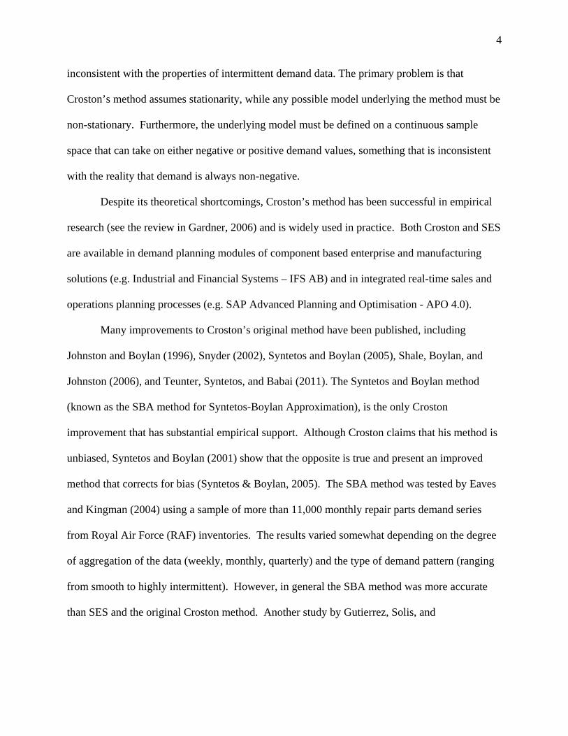
4
inconsistent with the properties of intermittent demand data The primary problem is that
Crostonrsquos method assumes stationarity while any possible model underlying the method must be
non-stationary Furthermore the underlying model must be defined on a continuous sample
space that can take on either negative or positive demand values something that is inconsistent
with the reality that demand is always non-negative
Despite its theoretical shortcomings Crostonrsquos method has been successful in empirical
research (see the review in Gardner 2006) and is widely used in practice Both Croston and SES
are available in demand planning modules of component based enterprise and manufacturing
solutions (eg Industrial and Financial Systems ndash IFS AB) and in integrated real-time sales and
operations planning processes (eg SAP Advanced Planning and Optimisation - APO 40)
Many improvements to Crostonrsquos original method have been published including
Johnston and Boylan (1996) Snyder (2002) Syntetos and Boylan (2005) Shale Boylan and
Johnston (2006) and Teunter Syntetos and Babai (2011) The Syntetos and Boylan method
(known as the SBA method for Syntetos-Boylan Approximation) is the only Croston
improvement that has substantial empirical support Although Croston claims that his method is
unbiased Syntetos and Boylan (2001) show that the opposite is true and present an improved
method that corrects for bias (Syntetos amp Boylan 2005) The SBA method was tested by Eaves
and Kingman (2004) using a sample of more than 11000 monthly repair parts demand series
from Royal Air Force (RAF) inventories The results varied somewhat depending on the degree
of aggregation of the data (weekly monthly quarterly) and the type of demand pattern (ranging
from smooth to highly intermittent) However in general the SBA method was more accurate
than SES and the original Croston method Another study by Gutierrez Solis and
5
Mukhopadhyay (2008) reaches similar conclusions In the empirical study below all three
parametric alternatives are tested SES Crostonrsquos original method and the SBA method
Given the parametric point forecasts a demand distribution is needed to set inventory
levels Both the Poisson and Bernoulli processes have been found to fit demand arrivals ie the
probability of demand occurring (Dunsmuir amp Snyder 1989 Willemain Smart Shockor amp
DeSautels 1994 Janssen 1998 Eaves 2002) Regarding the size of demand when it occurs
various suggestions have been made for distributions that are either monotonically decreasing or
unimodal positively skewed With Poisson or Bernoulli arrivals of demands and any distribution
of demand sizes the resulting distribution of total demand over a fixed lead time is compound
Poisson or compound Bernoulli respectively Compound Poisson distributions are simpler and
have empirical evidence in their support (eg Boylan amp Syntetos 2008) In this empirical
study demand is modeled with the Negative Binomial Distribution (NBD) which performed
well in the empirical study by Snyder Ord and Beaumont (2012) The NBD is a compound
distribution in which the number of demands in each period is Poisson distributed with random
demand sizes governed by a logarithmic distribution
As the data become more erratic the true demand size distribution may not conform to
any standard theoretical distribution and it may be that non-parametric approaches (that do not
rely upon any underlying distributional assumption) may improve stock control Numerous
bootstrapping methods are available to randomly sample (with or without replacement)
observations from demand history to build a histogram of the lead-time demand distribution
Alternative bootstrapping methods are found in Efron (1979) Snyder (2002) Willemain Smart
and Schwarz (2004 hereafter WSS) Porras and Dekker (2008) Teunter and Duncan (2009)
Zhou and Viswanathan (2011) and Snyder et al (2012) The most robust bootstrapping method
6
appears to be that of WSS a method patented earlier by Willemain and Smart (2001) WSS is
tested in this paper further discussion on the justification for excluding other bootstrapping
alternatives follows in the next section
In a large empirical study WSS claims significant improvements in forecasting accuracy
over both SES and Crostonrsquos estimator However Gardner and Koehler (2005) criticize this
study because the authors do not use the correct lead time demand distribution for either SES or
Crostonrsquos method and they do not consider published improvements to Crostonrsquos method such
as the SBA method (see Willemain et al 2005 for a rejoinder) These mistakes are corrected in
this empirical study
One empirical study by Teunter and Duncan (2009) is similar to the one described in
this paper Using a sample of demand series for military spare parts Teunter and Duncan
compare the inventory and service tradeoffs that result from forecasting with the same
parametric methods tested below They also test a simple bootstrapping method in which they
sample lead time demand with replacement to estimate mean and variance which are then fed
into a normal distribution to set stock levels Reliance on the normal distribution defeats the
purpose of bootstrapping which does not require a distributional assumption
13 Organization of the Paper
Section 2 explains the parametric and bootstrapping methods Section 3 discusses the
data tested performance measurement and simulation procedures Empirical results are given in
Section 4 in contrast to most previous research in intermittent demand forecasting results are
presented in terms of stock control performance rather than forecast accuracy Section 5
7
discusses implications of the results followed by conclusions and opportunities for further
research in Section 6
2 Forecasting intermittent demand
21 Parametric Forecasting
Simple exponential smoothing (SES) is written
1)1( ttt SXS (1)
where is the smoothing parameter is the observed value of both zero and nonzero demand
and is the smoothed average as well as the forecast for next period Although SES is widely
used to forecast intermittent demand the method has important limitations Exponential
smoothing weights recent data more heavily which produces forecasts that are biased high just
after a demand occurs and biased low just before a demand Replenishment quantities are likely
to be determined by forecasts made just after a demand resulting in unnecessarily high stock
levels most of the time
tX
tS
In an attempt to compensate for these problems Crostonrsquos (1972) method forecasts two
components of the time series separately the observed value of nonzero demand ( ) and the
inter-arrival time of transactions ( ) The smoothed estimates are denoted and
respectively
tD
PtQ tZ t
1)1( ttt ZDZ (2)
1 )1( ttt PQP (3)
Croston assumes that the value of the smoothing parameter is the same in both
equations The estimate of demand per unit time ie the forecast for next period ( ) is then tY
8
ttt PZY (4)
If there is no demand in a period and are unchanged Note that when demand
occurs every period the Croston method gives the same forecasts as conventional SES Thus the
same method can be used for both intermittent and non-intermittent demands
tZ tP
Syntetos and Boylan (2001) show that is biased to over-forecast Later Syntetos and
Boylan (2005) developed the SBA method (for Syntetos-Boylan Approximation) a modified
version of equation (4) that is approximately unbiased
tY
))(21( ttt PZY (5)
SES Croston and SBA are used below to forecast demand over the lead time plus review
period As recommended by Syntetos and Boylan (2006) on the grounds of simplicity the
variance of the forecast errors is estimated by the exponentially smoothed mean squared error
(MSE) over the lead time plus review period
22 Non-Parametric Forecasting
Non-parametric or bootstrapping approaches to forecasting permit a reconstruction of the
empirical distribution of the data thus making distributional assumptions redundant
Bootstrapping works by taking many random samples from a larger sample or from a population
itself These samples may be different from each other and from the population and they are
used to build up a histogram of the distribution of inventory demands during lead time
Statistics such as the mean and variance of lead-time demand are computed directly from the
histogram rather than inferred from a theoretical distribution
The WSS method is an advanced form of bootstrapping that captures the autocorrelation
between demand realizations and can produce values that have not appeared in the history The
9
method estimates transition probabilities in a two-state (zero vs non-zero) Markov model and
uses that model to generate a sequence of zero and non-zero demand occurrences The non-zero
occurrences are then assigned a positive value (demand) by using an ad-hoc method of ldquojitteringrdquo
proposed by the authors The WSS method works according to the following steps which are
found in both WSS (2004) and Willemain and Smart (2001)
1 Obtain historical demand data in chosen time buckets (eg days weeks months) 2 Estimate transition probabilities for a two-state (zero vs non-zero) Markov model 3 Conditional on last observed demand use the Markov model to generate a sequence of
zeronon-zero values over the forecast horizon (lead time) 4 Replace every non-zero state marker with a numerical value sampled at random with
replacement from the set of observed non-zero demands 5 ldquoJitterrdquo the non-zero demand values X When X is selected at random generate a
realization of a standard normal random deviate Z The jittered value is )INT(1 X Z X unless the result is less than or equal to zero in which case the
jittered value is simply X 6 Sum the forecast values over the horizon to get one predicted value of lead time demand
(LTD)
Porras and Dekker (2008) propose an empirical method based on the construction of a
histogram of demands over the lead time (L) A block of L consecutive demand observations is
sampled repeatedly with replacement Such a procedure results in capturing the potential auto-
correlation of the demand data The method is intuitively appealing and links naturally to stock
control However the method cannot extrapolate beyond previous demands (an important
advantage of WSS) making it difficult to attain realistically high service level targets
10
Preliminary results not reported here show poor performance of the Porras and Decker method
which is not considered further
Viswanathan and Zhou (2008) claim an improvement to the WSS bootstrapping
procedure The key difference is that instead of the two-state Markov chain used by WSS the
historical inter-demand interval distribution generates demand arrivals However this procedure
is heavily dependent upon lengthy demand histories that are not often available Zhou and
Viswanathan (2011) compare their procedure to parametric methods on empirical data and find
the parametric methods are more accurate They attribute the inferior performance of the
bootstrapping method to the short demand histories available and this approach is not considered
further
Finally a parametric bootstrapping method proposed by Snyder (2002) was shown to
perform well on a few SKUs However we did not consider the Snyder method due to its
constraining theoretical assumptions that defy the purpose of using bootstrapping procedures in
the first place
3 Experimental design
31 Data
Forecasting performance is tested in the data described in Tables 1 ndash 2 (all data are
available from the corresponding author) The jewelry data are one year of weekly retail
demands for an inexpensive line of costume jewelry the distribution of demand intervals is
relatively compact around a median of 44 weeks and most demands are for one or two units
Stock replenishment lead-times in the jewelry data are one week A Japanese manufacturer
supplied the electronics data which consists of four years of monthly demand histories for spare
11
parts used in European support operations The median demand interval is relatively short at 26
months but both demand intervals and sizes are skewed right due to outliers in most time series
Lead-times in the electronics data are three months which makes stock control far more difficult
than in the jewelry data
------------------------------
Insert Table 1 Here ------------------------------
------------------------------ Insert Table 2 Here
------------------------------
32 Performance Measurement
Syntetos and Boylan (2006) and Syntetos Nikolopoulos and Boylan (2010) demonstrate
that there is little relationship between traditional measures of forecast accuracy such as the
mean error and stock control performance as measured by inventory investment and customer
service (For a general discussion of the organizational and inventory implications of forecast
errors refer to Sanders amp Graman 2009) Therefore accuracy measures are bypassed in this
study and forecasting is evaluated by its direct effects on stock control Gardner (1990 2006)
recommends the use of tradeoff curves for this purpose and that example is followed here by
computing tradeoffs between total inventory investment and customer service
Another suggestion for evaluating performance is the use of average regret metrics (Sani
and Kingsman 1997) or implied stock-holdings that are based on a calculation of the exact
safety margin providing a maximum stock-out of zero (Eaves and Kingsman 2004) An
alternative formulation involves fixing a target service measure and searching for the investment
necessary to hit the target However tradeoff curves are the most realistic representation of the
12
various methodsrsquo comparative performance and the most meaningful one from a practitioner
perspective
Performance is simulated using a periodic order-up-to-level stock control system which
is widely used in practice because it requires optimization of only one parameter the order-up-
to-level The stock control system is designed to meet a target fraction of replenishment cycles
in which total demand can be delivered from stock This fraction is called the cycle service level
(CSL) (ie the probability of no stock-outs during a replenishment cycle) During out-of-sample
testing the forecasting methods are used to compute weekly or monthly order-up-to-levels that
attempt to meet four CSL targets 85 90 95 and 99 Other service measures (like the
most commonly used fill rate for example) are not considered because bootstrapping does not
allow direct calculation of such measures
For the parametric methods the order-up-to-level in each period is computed as the
inverse of the cumulative distribution function of demand over the lead time plus one review
period Replenishment decisions take place at the end of every period (week or month) so the
review period is set equal to one Demands are assumed to follow the Negative Binomial
Distribution (NBD) One difficulty with the NBD is that it requires the variance to be greater
than the mean in the few cases where the reverse was true the variance is set equal to 11 times
the mean Although this may look ad hoc Sani (1995) shows that it produces robust results
33 Model-Fitting and Forecasting
To test the parametric forecasting methods the demand history for each SKU is split into
two parts within sample (for initialization and optimization purposes) and out-of-sample (for
reporting performance) The first 12 observations are used as an initialization sample to compute
13
an average for the beginning level of demand and in the case of Crostonrsquos method the beginning
demand size and interval (expressed also as averages of the corresponding variables over the
initialization block) To make the most use of the data available the optimization block contains
the initialization block and extends it by the same number of periods That is the first 24
observations are used as an optimization sample to select the smoothing parameter over the range
005 to 030 (in steps of 001) that minimizes the mean squared error (MSE) per series (For more
details on the issue of optimization of parameters in an intermittent demand context please refer
to Petropoulos Nikolopoulos Spithourakis amp Assimakopoulos 2013) Variances are estimated
by the cumulative smoothed MSE using a fixed smoothing parameter of 025 analysis not
reported here indicates that this value performs well In Crostonrsquos original method the same
smoothing parameter updates both demand size and interval but a separate smoothing parameter
for each one is used here following Schultzrsquos (1987) advice that separate parameters lead to
better forecast accuracy For the WSS method the within sample data are used to compute an
initial value for the order-up-to-level which is then updated weekly or monthly Out-of-sample
testing starts at period 25 so there are 28 out-of-sample observations in each jewelry series and
24 in each electronics series
4 Empirical results
Three performance measures are reported for every combination of forecasting method
dataset and target CSL First total inventory investment is computed by pricing each SKU by
unit cost and summing across all SKUs Second the achieved CSL is computed as the actual
percentage of replenishment cycles in which demand is satisfied directly from stock on hand
Finally total backorders are computed by averaging backorder values over time (weeks or
14
months) for each SKU and then summing across all SKUs These measures are presented in the
form of tradeoff curves showing achieved CSL and total backorders as a function of total
investment Each curve has four plotting symbols corresponding to the four CSL targets
41 Jewelry Data
In the jewelry data Figure 1 shows tradeoff curves between investment and CSL All
forecasting methods achieve CSLs slightly larger than the 99 target (with the exception of SES
that just falls short of that) but achieved levels are significantly greater than targets of 85
90 and 95 The descriptive statistics presented in Table 2 indicate that the jewelry data are
neither particularly intermittent nor erratic the latter referring to the variability of the demand
sizes Thus the NBD provides a good fit to the empirical data and the parametric methods
produce very similar CSL tradeoff curves (with the SBA and Croston being indicated as the
lsquobestrsquo approaches) The curve for the WSS method runs above the parametric curves at targets
of 95 and 99 and gives a slightly better CSL for any level of investment greater than about
$130000 For example at an investment of $175000 WSS adds about one percentage point to
CSL compared to the other methods Inventory investment vs backorders are plotted in Figure 2
and again the parametric methods produce similar results while the WSS method yields lower
backorder values for any investment greater than $130000
------------------------------ Insert Figure 1 Here
------------------------------
------------------------------ Insert Figure 2 Here
------------------------------
15
42 Electronics Data
The electronics data are more erratic than the jewelry data and the results are
considerably different In Figure 3 all methods achieve CSLs greater than the 85 target and
all methods are close to the 90 target However at the 95 and 99 target all methods
significantly underperform For example when SES is run with a target of 99 the achieved
CSL is only 95 Outliers in the electronics data make it extremely difficult to estimate the
parameters of the demand distribution and hit the CSL targets
The Croston method consistently gives better CSL performance than the SBA method
even though SBA was designed to improve on Croston The problem is that the Croston method
is biased high which increases both customer service and inventory investment SES produces
the best CSL tradeoff curve through an investment of about euro48 million and thereafter WSS is
marginally better At an investment of euro40 million SES yields a CSL about one percentage
point better than WSS But at an investment of euro65 million WSS is about one-half percentage
point better than SES
Differences in backorder performance are more significant In Figure 4 all parametric
methods produce smaller backorders than WSS at all levels of investment For example at an
investment of euro35 million SES backorders are euro14 million compared to euro22 million for WSS
SES yields the smallest backorders though an investment of about euro50 million thereafter the
SBA method is best followed closely by Croston
------------------------------ Insert Figure 3 Here
------------------------------
------------------------------ Insert Figure 4 Here
------------------------------
16
5 Implications and practical considerations
The jewelry data are relatively well behaved with moderately intermittent demands and
short lead times all parametric methods give similar performance and the WSS bootstrapping
method is marginally better than the parametric methods The electronics data are more difficult
to forecast because they are more intermittent contain more outliers and have longer lead times
Under these conditions we might expect WSS to perform better than the parametric methods
but this did not happen In the electronics data all parametric methods give significantly better
backorder performance than WSS
Willemain et al (2004) claimed that an important advantage related to the use of
bootstrapping is its attractiveness to practitioners ldquoUsers intuitively grasp the simple
procedural explanation of how the bootstrap works Their comfort with the bootstrap approach
may derive from the concrete algorithmic nature of computational inference in contrast to the
more abstract character of traditional mathematical approaches to statistical inferencerdquo This
claim may be true for the general bootstrapping concept but the details of the WSS method such
as the use of transition probabilities and Markov models are more complicated and difficult to
understand than any of the parametric methods tested
Another consideration in evaluating the WSS procedure is that demand forecasts are
often subject to judgmental adjustments (Syntetos Nikolopoulos Boylan Fildes amp Goodwin
2009) Such adjustments can be beneficial especially when they are based on information not
available to the forecasting model However adjustments can be unnecessary or even harmful
when they are applied without an understanding of how the forecasts were produced Simple
methods should result in fewer damaging judgmental interventions
17
Although the parametric forecasting methods are simple their interactions with stock
control are not Many authors have pointed out that forecast errors may seriously distort
projections of customer service levels in an intermittent demand context The fundamental
problem is that inventory theory has been developed upon the assumptions of known moments of
the hypothesized demand distribution Although no concrete theory has been developed in this
area there is an expectation that parametric estimators will sometimes under-achieve the
specified targets A common reaction from practitioners is to incorporate some bias in the
forecasts to avoid running out of stock However such adjustments are not straightforward since
the variance of the estimates (sampling error of the mean) is also affected leading to confusion
about the effects on performance of the system
The application of bootstrapping is relatively straightforward under the CSL constraint
but such is not the case should other service measures and cost criteria be considered Parametric
theory despite its shortcomings does provide guidelines for optimization of the stock control
system under a wide range of objectives andor constraints More research is needed to extend
the capacity of bootstrapping to match parametric theory Consider for example the specification
of a fill-rate target as opposed to the CSL in a practical setting bootstrapping cannot be used
directly to meet a fill-rate target
6 Conclusions and future research
The WSS method of bootstrapping does have advantages most notably the ability to
simulate demand values that have not appeared in history However it is questionable whether
the WSS method is worth the considerable added complexity Parametric methods are simpler
18
and the simplest method of all SES performs well In the messy electronics data SES produces
fewer backorders than WSS at all levels of inventory investment
Parametric methods require less computing power which is important when demands for
very large numbers of SKUs have to be forecast Parametric methods also require less specialist
knowledge and thus are more transparent and more resistant to potentially damaging judgmental
interventions
Teunter and Duncan (2009) observed that analytical projections of customer service are
often different from empirical results in an intermittent demand context a conclusion that applies
to this study as well In the jewelry data achieved CSLs for all methods were significantly
greater than targets of 85 90 and 95 In the electronics data achieved CSLs were
significantly less than targets of 95 and 99 The difference between target and achieved
CSLs are attributed to errors in estimating the parameters of the demand distribution if these
parameters were known achieved CSLs should correspond to the targets
There are several opportunities for further research in intermittent demand forecasting
The M and M3 forecasting competitions (Makridakis Andersen Carbone Fildes Hibon
Lewandowski Newton Parzen amp Winkler 1982 and Makridakis amp Hibon 2000 respectively)
did not consider intermittent demand data Future competitions should include such data
An alternative strategy to deal with intermittent demand patterns is to aggregate demand
in lower-frequency time buckets thereby reducing the presence of zero observations Temporal
aggregation is a practice employed in many real world settings but there has been no research
apart from a few studies (Nikolopoulos Syntetos Boylan Petropoulos amp Assimakopoulos
2011 Babai Ali amp Nikolopoulos 2012 Spithourakis Petropoulos Nikolopoulos amp
Assimakopoulos 2012)
19
Another research opportunity is to consider stationary models for intermittent demand
forecasting rather than restricting attention to models based on Crostonrsquos method For example
Poisson autoregressive models have been suggested by Shenstone and Hyndman (2005) Models
based on a variety of count probability distributions coupled with dynamic specifications to
account for potential serial correlation have recently been analyzed by Snyder et al (2012)
although the authors made no attempt to evaluate stock control results Further development and
testing of such models in the context of stock control is the next step in our research
Finally we acknowledge that the bootstrapping algorithm considered in this paper is the
exclusive property of Smart Software Inc under US Patent 6205431 B1 Use in this paper was
permitted by a special licensing arrangement with Smart Software and does not imply a public
license to use the algorithm According to Smart Software ldquoThis algorithm differs in several
important ways from the commercial implementation in the SmartForecaststrade software so
conclusions about the performance of the algorithm implemented here cannot be extrapolated to
the performance of SmartForecaststrade Further Smart Software provided no oversight or
guidance in implementing the algorithmrdquo
Note At least one of the authors has read each reference in this paper We contacted
Ruud Teunter and Thomas Willemain to ensure that their work was properly summarized
References
Babai MZ Ali M amp Nikolopoulos K (2012) Impact of temporal aggregation on stock
control performance of intermittent demand estimators OMEGA international Journal of
Management Science 40(6) 713-721
20
Boylan JE amp Syntetos AA (2008) Forecasting for inventory management of service parts In
DNP Murthy amp KAH Kobbacy (Eds) Complex system maintenance handbook London
Springer Verlag 479-508
Brown RG (1959) Statistical forecasting for inventory control New York McGraw-Hill
Cattani KD Jacobs FR amp Schoenfelder J (2011) Common inventory modelling assumptions
that fall short Arborescent networks Poisson demand and single echelon approximations Journal of
Operations Management 29(5) 488-499
Croston JD (1972) Forecasting and stock control for intermittent demands Operational
Research Quarterly 23(3) 289-304
Deloitte (2011) The service revolution in global manufacturing industries New York Deloitte
Research
Dunsmuir WTM amp Snyder RD (1989) Control of inventories with intermittent demand
European Journal of Operational Research 40(1) 16-21
Eaves AHC (2002) Forecasting for the ordering and stock holding of consumable spare
parts Doctoral dissertation Lancaster University Lancaster UK
21
Eaves AHC amp Kingsman BG (2004) Forecasting for the ordering and stockholding of spare
parts Journal of the Operational Research Society 55(4) 431-437
Efron B (1979) Bootstrap methods another look at the jackknife Annals of Statistics 7(1) 1-
26
Gardner ES (1990) Evaluating forecast performance in an inventory control system
Management Science 36(4) 490-499
Gardner ES (2006) Exponential smoothing the state of the art - part II International Journal
of Forecasting 22(4) 637ndash666
Gardner ES amp Koehler AB (2005) Comments on a patented bootstrapping method for
forecasting intermittent demand International Journal of Forecasting 21(3) 617-618
Gutierrez RS Solis AO amp Mukhopadhyay S (2008) Lumpy demand forecasting using
neural networks International Journal of Production Economics 111(2) 409-420
Hinton Jr HL (1999) Defense inventory continuing challenges in managing inventories and
avoiding adverse operational effects Washington DC US General Accounting Office
22
Janssen FBSLP (1998) Inventory management systems control and information issues
Doctoral dissertation Centre for Economic Research Tilburg University Tilburg The
Netherlands
Johnston F R amp Boylan J E (1996) Forecasting for items with intermittent demand Journal
of the Operational Research Society 47(1) 113ndash121
Johnston FR Boylan JE amp Shale EA (2003) An examination of the size of orders from
customers their characterization and the implications for inventory control of slow moving
items Journal of the Operational Research Society 54(8) 833-837
Makridakis S Andersen A Carbone R Fildes R Hibon M Lewandowski R Newton J
Parzen E amp Winkler R (1982) The accuracy of extrapolation (time series) methods results of
a forecasting competition Journal of Forecasting 1(2) 111-153
Makridakis S amp Hibon M (2000) The M3-competition results conclusions and implications
International Journal of Forecasting 16(4) 451-476
Molenaers A Baets H Pintelon L amp Waeyenberg G (2010) Criticality classification of
spare parts A case study Preprints of the 16th International Working Seminar on Production
Economics Innsbruck Austria
23
Nikolopoulos K Syntetos AA Boylan JE Petropoulos F amp Assimakopoulos V (2011) An
aggregate ndash disaggregate intermittent demand approach (ADIDA) to forecasting An empirical
proposition and analysis Journal of the Operational Research Society 62(3) 544-554
Petropoulos F Nikolopoulos K Spithourakis GP amp Assimakopoulos V (2013) Empirical
heuristics for improving intermittent demand forecasting Industrial Management amp Data
Systems 113(5) 683-696
Porras EM amp Dekker R (2008) An inventory control system for spare parts at a refinery An
empirical comparison of different reorder point methods European Journal of Operational
Research 184(1) 101-132
Rao A V (1973) A comment on Forecasting and stock control for intermittent demands
Operational Research Quarterly 24(4) 639-640
Sanders NR amp Graman GA (2009) Quantifying costs of forecast errors A case study of the
warehouse environment OMEGA The International Journal of Management Science 37(1)
116-125
Sani B (1995) Periodic inventory control systems and demand forecasting methods for low
demand items Doctoral dissertation Lancaster University Lancaster UK
24
Sani B amp Kingsman BG (1997) Selecting the best periodic inventory control and demand
forecasting methods for low demand items Journal of the Operational Research Society 48 (7)
700-713
Schultz CR (1987) Forecasting and inventory control for sporadic demand under periodic
review Journal of the Operational Research Society 38(5) 453-458
Shale EA Boylan JE amp Johnston FR (2006) Forecasting for intermittent demand the
estimation of an unbiased average Journal of the Operational Research Society 57(5) 588-592
Shenstone L amp Hyndman RJ (2005) Stochastic models underlying Crostonrsquos method for
intermittent demand forecasting Journal of Forecasting 24(6) 389-402
Snyder R (2002) Forecasting sales of slow and fast moving inventories European Journal of
Operational Research 140(3) 684-699
Snyder R Ord K amp Beaumont A (2012) Forecasting the intermittent demand for slow-
moving inventories a modelling approach International Journal of Forecasting 28(2) 485-496
Spithourakis GP Petropoulos F Nikolopoulos K amp Assimakopoulos V (2012) A systemic
view of the ADIDA framework IMA Journal of Management Mathematics advance online
publication doi101093imamandps031
25
Syntetos AA amp Boylan JE (2001) On the bias of intermittent demand estimates
International Journal of Production Economics 71(1-3) 457-466
Syntetos AA amp Boylan JE (2005) The Accuracy of Intermittent Demand Estimates
International Journal of Forecasting 21(2) 303-314
Syntetos AA amp Boylan JE (2006) On the stock control performance of intermittent demand
estimators International Journal of Production Economics 103(1) 36-47
Syntetos AA Keyes M amp Babai MZ (2009) Demand categorisation in a European spare
parts logistics network International Journal of Operations and Production Management 29(3)
292-316
Syntetos AA Nikolopoulos K Boylan JE Fildes R amp Goodwin P (2009) The ffects of
integrating management judgement into intermittent demand forecasts International Journal of
Production Economics 118(1) 72-81
Syntetos AA Nikolopoulos K amp Boylan JE (2010) Judging the judges through accuracy-
implication metrics The case of inventory forecasting International Journal of Forecasting 26(1)
134-143
26
Teunter R amp Duncan L (2009) Forecasting intermittent demand A comparative study
Journal of the Operational Research Society 60(3) 321-329
Teunter R Syntetos AA amp Babai MZ (2011) Intermittent demand Linking forecasting to
inventory obsolescence European Journal of Operational Research 214(3) 606-615
Viswanathan S amp Zhou CX (2008) A new bootstrapping based method for forecasting and
safety stock determination for intermittent demand items Working paper Nanyang Business
School Nanyang Technological University Singapore
Willemain TR amp Smart CN (2001) United States Patent 6205431 B1 System and method
for forecasting intermittent demand Available at httppatftusptogov
Willemain TR Smart CN Shockor JH amp DeSautels PA (1994) Forecasting intermittent
demand in manufacturing A comparative evaluation of Crostonrsquos method International Journal
of Forecasting 10(4) 529-538
Willemain TR Smart CN amp Schwarz HF (2004) A new approach to forecasting
intermittent demand for service parts inventories International Journal of Forecasting 20(3)
375-387
27
Willemain TR Smart CN amp Schwarz HF (2005) Authorrsquos response to Koehler and
Gardner International Journal of Forecasting 21(3) 619-620
Zhou CX amp Viswanathan S (2011) Comparison of a new bootstrapping method with
parametric approaches for safety stock determination in service parts inventory systems
International Journal of Production Economics 133(1) 481-485
28
TABLES
Table 1 Jewelry data - 52 weeks of demands for 4076 SKUs
Mean Std Dev Mean Std Dev Mean Std DevMinimum 13 06 10 00 01 0325th percentile 33 26 11 03 02 04Median 44 37 12 04 03 0575th percentile 56 50 14 07 04 07Maximum 87 130 32 37 22 25
Demand interval Demand size Demand per period
Table 2 Electronics data - 48 months of demands for 3055 SKUs
Mean Std Dev Mean Std Dev Mean Std DevMinimum 10 00 10 00 00 0225th percentile 15 10 35 30 09 22Median 26 23 59 62 21 4575th percentile 47 44 121 139 60 105Maximum 240 325 53662 91493 53662 38584
Demand interval Demand size Demand per period
29
FIGURES
Figure 1 Jewelry data - investment vs CSL
88
90
92
94
96
98
100
50 100 150 200 250 300
Inventory investment (K$)
Ach
ieve
d C
SL
SES
Croston
SBA
WSS
Figure 2 Jewelry data - investment vs backorders
0
2
4
6
8
10
12
50 100 150 200 250 300
Inventory investment (K$)
Bac
kord
ers
(K$)
SES
Croston
SBA
WSS
30
Figure 3 Electronics data - investment vs CSL
84
86
88
90
92
94
96
98
30 35 40 45 50 55 60 65 70 75 80
Inventory investment (Meuro)
Ach
ieve
d C
SL
SES
Croston
SBA
WSS
Figure 4 Electronics data - investment vs backorders
00
05
10
15
20
25
30 35 40 45 50 55 60 65 70 75 80
Inventory investment (Meuro)
Bac
kord
ers
(Meuro)
SES
Croston
SBA
WSS

6
appears to be that of WSS a method patented earlier by Willemain and Smart (2001) WSS is
tested in this paper further discussion on the justification for excluding other bootstrapping
alternatives follows in the next section
In a large empirical study WSS claims significant improvements in forecasting accuracy
over both SES and Crostonrsquos estimator However Gardner and Koehler (2005) criticize this
study because the authors do not use the correct lead time demand distribution for either SES or
Crostonrsquos method and they do not consider published improvements to Crostonrsquos method such
as the SBA method (see Willemain et al 2005 for a rejoinder) These mistakes are corrected in
this empirical study
One empirical study by Teunter and Duncan (2009) is similar to the one described in
this paper Using a sample of demand series for military spare parts Teunter and Duncan
compare the inventory and service tradeoffs that result from forecasting with the same
parametric methods tested below They also test a simple bootstrapping method in which they
sample lead time demand with replacement to estimate mean and variance which are then fed
into a normal distribution to set stock levels Reliance on the normal distribution defeats the
purpose of bootstrapping which does not require a distributional assumption
13 Organization of the Paper
Section 2 explains the parametric and bootstrapping methods Section 3 discusses the
data tested performance measurement and simulation procedures Empirical results are given in
Section 4 in contrast to most previous research in intermittent demand forecasting results are
presented in terms of stock control performance rather than forecast accuracy Section 5
7
discusses implications of the results followed by conclusions and opportunities for further
research in Section 6
2 Forecasting intermittent demand
21 Parametric Forecasting
Simple exponential smoothing (SES) is written
1)1( ttt SXS (1)
where is the smoothing parameter is the observed value of both zero and nonzero demand
and is the smoothed average as well as the forecast for next period Although SES is widely
used to forecast intermittent demand the method has important limitations Exponential
smoothing weights recent data more heavily which produces forecasts that are biased high just
after a demand occurs and biased low just before a demand Replenishment quantities are likely
to be determined by forecasts made just after a demand resulting in unnecessarily high stock
levels most of the time
tX
tS
In an attempt to compensate for these problems Crostonrsquos (1972) method forecasts two
components of the time series separately the observed value of nonzero demand ( ) and the
inter-arrival time of transactions ( ) The smoothed estimates are denoted and
respectively
tD
PtQ tZ t
1)1( ttt ZDZ (2)
1 )1( ttt PQP (3)
Croston assumes that the value of the smoothing parameter is the same in both
equations The estimate of demand per unit time ie the forecast for next period ( ) is then tY
8
ttt PZY (4)
If there is no demand in a period and are unchanged Note that when demand
occurs every period the Croston method gives the same forecasts as conventional SES Thus the
same method can be used for both intermittent and non-intermittent demands
tZ tP
Syntetos and Boylan (2001) show that is biased to over-forecast Later Syntetos and
Boylan (2005) developed the SBA method (for Syntetos-Boylan Approximation) a modified
version of equation (4) that is approximately unbiased
tY
))(21( ttt PZY (5)
SES Croston and SBA are used below to forecast demand over the lead time plus review
period As recommended by Syntetos and Boylan (2006) on the grounds of simplicity the
variance of the forecast errors is estimated by the exponentially smoothed mean squared error
(MSE) over the lead time plus review period
22 Non-Parametric Forecasting
Non-parametric or bootstrapping approaches to forecasting permit a reconstruction of the
empirical distribution of the data thus making distributional assumptions redundant
Bootstrapping works by taking many random samples from a larger sample or from a population
itself These samples may be different from each other and from the population and they are
used to build up a histogram of the distribution of inventory demands during lead time
Statistics such as the mean and variance of lead-time demand are computed directly from the
histogram rather than inferred from a theoretical distribution
The WSS method is an advanced form of bootstrapping that captures the autocorrelation
between demand realizations and can produce values that have not appeared in the history The
9
method estimates transition probabilities in a two-state (zero vs non-zero) Markov model and
uses that model to generate a sequence of zero and non-zero demand occurrences The non-zero
occurrences are then assigned a positive value (demand) by using an ad-hoc method of ldquojitteringrdquo
proposed by the authors The WSS method works according to the following steps which are
found in both WSS (2004) and Willemain and Smart (2001)
1 Obtain historical demand data in chosen time buckets (eg days weeks months) 2 Estimate transition probabilities for a two-state (zero vs non-zero) Markov model 3 Conditional on last observed demand use the Markov model to generate a sequence of
zeronon-zero values over the forecast horizon (lead time) 4 Replace every non-zero state marker with a numerical value sampled at random with
replacement from the set of observed non-zero demands 5 ldquoJitterrdquo the non-zero demand values X When X is selected at random generate a
realization of a standard normal random deviate Z The jittered value is )INT(1 X Z X unless the result is less than or equal to zero in which case the
jittered value is simply X 6 Sum the forecast values over the horizon to get one predicted value of lead time demand
(LTD)
Porras and Dekker (2008) propose an empirical method based on the construction of a
histogram of demands over the lead time (L) A block of L consecutive demand observations is
sampled repeatedly with replacement Such a procedure results in capturing the potential auto-
correlation of the demand data The method is intuitively appealing and links naturally to stock
control However the method cannot extrapolate beyond previous demands (an important
advantage of WSS) making it difficult to attain realistically high service level targets
10
Preliminary results not reported here show poor performance of the Porras and Decker method
which is not considered further
Viswanathan and Zhou (2008) claim an improvement to the WSS bootstrapping
procedure The key difference is that instead of the two-state Markov chain used by WSS the
historical inter-demand interval distribution generates demand arrivals However this procedure
is heavily dependent upon lengthy demand histories that are not often available Zhou and
Viswanathan (2011) compare their procedure to parametric methods on empirical data and find
the parametric methods are more accurate They attribute the inferior performance of the
bootstrapping method to the short demand histories available and this approach is not considered
further
Finally a parametric bootstrapping method proposed by Snyder (2002) was shown to
perform well on a few SKUs However we did not consider the Snyder method due to its
constraining theoretical assumptions that defy the purpose of using bootstrapping procedures in
the first place
3 Experimental design
31 Data
Forecasting performance is tested in the data described in Tables 1 ndash 2 (all data are
available from the corresponding author) The jewelry data are one year of weekly retail
demands for an inexpensive line of costume jewelry the distribution of demand intervals is
relatively compact around a median of 44 weeks and most demands are for one or two units
Stock replenishment lead-times in the jewelry data are one week A Japanese manufacturer
supplied the electronics data which consists of four years of monthly demand histories for spare
11
parts used in European support operations The median demand interval is relatively short at 26
months but both demand intervals and sizes are skewed right due to outliers in most time series
Lead-times in the electronics data are three months which makes stock control far more difficult
than in the jewelry data
------------------------------
Insert Table 1 Here ------------------------------
------------------------------ Insert Table 2 Here
------------------------------
32 Performance Measurement
Syntetos and Boylan (2006) and Syntetos Nikolopoulos and Boylan (2010) demonstrate
that there is little relationship between traditional measures of forecast accuracy such as the
mean error and stock control performance as measured by inventory investment and customer
service (For a general discussion of the organizational and inventory implications of forecast
errors refer to Sanders amp Graman 2009) Therefore accuracy measures are bypassed in this
study and forecasting is evaluated by its direct effects on stock control Gardner (1990 2006)
recommends the use of tradeoff curves for this purpose and that example is followed here by
computing tradeoffs between total inventory investment and customer service
Another suggestion for evaluating performance is the use of average regret metrics (Sani
and Kingsman 1997) or implied stock-holdings that are based on a calculation of the exact
safety margin providing a maximum stock-out of zero (Eaves and Kingsman 2004) An
alternative formulation involves fixing a target service measure and searching for the investment
necessary to hit the target However tradeoff curves are the most realistic representation of the
12
various methodsrsquo comparative performance and the most meaningful one from a practitioner
perspective
Performance is simulated using a periodic order-up-to-level stock control system which
is widely used in practice because it requires optimization of only one parameter the order-up-
to-level The stock control system is designed to meet a target fraction of replenishment cycles
in which total demand can be delivered from stock This fraction is called the cycle service level
(CSL) (ie the probability of no stock-outs during a replenishment cycle) During out-of-sample
testing the forecasting methods are used to compute weekly or monthly order-up-to-levels that
attempt to meet four CSL targets 85 90 95 and 99 Other service measures (like the
most commonly used fill rate for example) are not considered because bootstrapping does not
allow direct calculation of such measures
For the parametric methods the order-up-to-level in each period is computed as the
inverse of the cumulative distribution function of demand over the lead time plus one review
period Replenishment decisions take place at the end of every period (week or month) so the
review period is set equal to one Demands are assumed to follow the Negative Binomial
Distribution (NBD) One difficulty with the NBD is that it requires the variance to be greater
than the mean in the few cases where the reverse was true the variance is set equal to 11 times
the mean Although this may look ad hoc Sani (1995) shows that it produces robust results
33 Model-Fitting and Forecasting
To test the parametric forecasting methods the demand history for each SKU is split into
two parts within sample (for initialization and optimization purposes) and out-of-sample (for
reporting performance) The first 12 observations are used as an initialization sample to compute
13
an average for the beginning level of demand and in the case of Crostonrsquos method the beginning
demand size and interval (expressed also as averages of the corresponding variables over the
initialization block) To make the most use of the data available the optimization block contains
the initialization block and extends it by the same number of periods That is the first 24
observations are used as an optimization sample to select the smoothing parameter over the range
005 to 030 (in steps of 001) that minimizes the mean squared error (MSE) per series (For more
details on the issue of optimization of parameters in an intermittent demand context please refer
to Petropoulos Nikolopoulos Spithourakis amp Assimakopoulos 2013) Variances are estimated
by the cumulative smoothed MSE using a fixed smoothing parameter of 025 analysis not
reported here indicates that this value performs well In Crostonrsquos original method the same
smoothing parameter updates both demand size and interval but a separate smoothing parameter
for each one is used here following Schultzrsquos (1987) advice that separate parameters lead to
better forecast accuracy For the WSS method the within sample data are used to compute an
initial value for the order-up-to-level which is then updated weekly or monthly Out-of-sample
testing starts at period 25 so there are 28 out-of-sample observations in each jewelry series and
24 in each electronics series
4 Empirical results
Three performance measures are reported for every combination of forecasting method
dataset and target CSL First total inventory investment is computed by pricing each SKU by
unit cost and summing across all SKUs Second the achieved CSL is computed as the actual
percentage of replenishment cycles in which demand is satisfied directly from stock on hand
Finally total backorders are computed by averaging backorder values over time (weeks or
14
months) for each SKU and then summing across all SKUs These measures are presented in the
form of tradeoff curves showing achieved CSL and total backorders as a function of total
investment Each curve has four plotting symbols corresponding to the four CSL targets
41 Jewelry Data
In the jewelry data Figure 1 shows tradeoff curves between investment and CSL All
forecasting methods achieve CSLs slightly larger than the 99 target (with the exception of SES
that just falls short of that) but achieved levels are significantly greater than targets of 85
90 and 95 The descriptive statistics presented in Table 2 indicate that the jewelry data are
neither particularly intermittent nor erratic the latter referring to the variability of the demand
sizes Thus the NBD provides a good fit to the empirical data and the parametric methods
produce very similar CSL tradeoff curves (with the SBA and Croston being indicated as the
lsquobestrsquo approaches) The curve for the WSS method runs above the parametric curves at targets
of 95 and 99 and gives a slightly better CSL for any level of investment greater than about
$130000 For example at an investment of $175000 WSS adds about one percentage point to
CSL compared to the other methods Inventory investment vs backorders are plotted in Figure 2
and again the parametric methods produce similar results while the WSS method yields lower
backorder values for any investment greater than $130000
------------------------------ Insert Figure 1 Here
------------------------------
------------------------------ Insert Figure 2 Here
------------------------------
15
42 Electronics Data
The electronics data are more erratic than the jewelry data and the results are
considerably different In Figure 3 all methods achieve CSLs greater than the 85 target and
all methods are close to the 90 target However at the 95 and 99 target all methods
significantly underperform For example when SES is run with a target of 99 the achieved
CSL is only 95 Outliers in the electronics data make it extremely difficult to estimate the
parameters of the demand distribution and hit the CSL targets
The Croston method consistently gives better CSL performance than the SBA method
even though SBA was designed to improve on Croston The problem is that the Croston method
is biased high which increases both customer service and inventory investment SES produces
the best CSL tradeoff curve through an investment of about euro48 million and thereafter WSS is
marginally better At an investment of euro40 million SES yields a CSL about one percentage
point better than WSS But at an investment of euro65 million WSS is about one-half percentage
point better than SES
Differences in backorder performance are more significant In Figure 4 all parametric
methods produce smaller backorders than WSS at all levels of investment For example at an
investment of euro35 million SES backorders are euro14 million compared to euro22 million for WSS
SES yields the smallest backorders though an investment of about euro50 million thereafter the
SBA method is best followed closely by Croston
------------------------------ Insert Figure 3 Here
------------------------------
------------------------------ Insert Figure 4 Here
------------------------------
16
5 Implications and practical considerations
The jewelry data are relatively well behaved with moderately intermittent demands and
short lead times all parametric methods give similar performance and the WSS bootstrapping
method is marginally better than the parametric methods The electronics data are more difficult
to forecast because they are more intermittent contain more outliers and have longer lead times
Under these conditions we might expect WSS to perform better than the parametric methods
but this did not happen In the electronics data all parametric methods give significantly better
backorder performance than WSS
Willemain et al (2004) claimed that an important advantage related to the use of
bootstrapping is its attractiveness to practitioners ldquoUsers intuitively grasp the simple
procedural explanation of how the bootstrap works Their comfort with the bootstrap approach
may derive from the concrete algorithmic nature of computational inference in contrast to the
more abstract character of traditional mathematical approaches to statistical inferencerdquo This
claim may be true for the general bootstrapping concept but the details of the WSS method such
as the use of transition probabilities and Markov models are more complicated and difficult to
understand than any of the parametric methods tested
Another consideration in evaluating the WSS procedure is that demand forecasts are
often subject to judgmental adjustments (Syntetos Nikolopoulos Boylan Fildes amp Goodwin
2009) Such adjustments can be beneficial especially when they are based on information not
available to the forecasting model However adjustments can be unnecessary or even harmful
when they are applied without an understanding of how the forecasts were produced Simple
methods should result in fewer damaging judgmental interventions
17
Although the parametric forecasting methods are simple their interactions with stock
control are not Many authors have pointed out that forecast errors may seriously distort
projections of customer service levels in an intermittent demand context The fundamental
problem is that inventory theory has been developed upon the assumptions of known moments of
the hypothesized demand distribution Although no concrete theory has been developed in this
area there is an expectation that parametric estimators will sometimes under-achieve the
specified targets A common reaction from practitioners is to incorporate some bias in the
forecasts to avoid running out of stock However such adjustments are not straightforward since
the variance of the estimates (sampling error of the mean) is also affected leading to confusion
about the effects on performance of the system
The application of bootstrapping is relatively straightforward under the CSL constraint
but such is not the case should other service measures and cost criteria be considered Parametric
theory despite its shortcomings does provide guidelines for optimization of the stock control
system under a wide range of objectives andor constraints More research is needed to extend
the capacity of bootstrapping to match parametric theory Consider for example the specification
of a fill-rate target as opposed to the CSL in a practical setting bootstrapping cannot be used
directly to meet a fill-rate target
6 Conclusions and future research
The WSS method of bootstrapping does have advantages most notably the ability to
simulate demand values that have not appeared in history However it is questionable whether
the WSS method is worth the considerable added complexity Parametric methods are simpler
18
and the simplest method of all SES performs well In the messy electronics data SES produces
fewer backorders than WSS at all levels of inventory investment
Parametric methods require less computing power which is important when demands for
very large numbers of SKUs have to be forecast Parametric methods also require less specialist
knowledge and thus are more transparent and more resistant to potentially damaging judgmental
interventions
Teunter and Duncan (2009) observed that analytical projections of customer service are
often different from empirical results in an intermittent demand context a conclusion that applies
to this study as well In the jewelry data achieved CSLs for all methods were significantly
greater than targets of 85 90 and 95 In the electronics data achieved CSLs were
significantly less than targets of 95 and 99 The difference between target and achieved
CSLs are attributed to errors in estimating the parameters of the demand distribution if these
parameters were known achieved CSLs should correspond to the targets
There are several opportunities for further research in intermittent demand forecasting
The M and M3 forecasting competitions (Makridakis Andersen Carbone Fildes Hibon
Lewandowski Newton Parzen amp Winkler 1982 and Makridakis amp Hibon 2000 respectively)
did not consider intermittent demand data Future competitions should include such data
An alternative strategy to deal with intermittent demand patterns is to aggregate demand
in lower-frequency time buckets thereby reducing the presence of zero observations Temporal
aggregation is a practice employed in many real world settings but there has been no research
apart from a few studies (Nikolopoulos Syntetos Boylan Petropoulos amp Assimakopoulos
2011 Babai Ali amp Nikolopoulos 2012 Spithourakis Petropoulos Nikolopoulos amp
Assimakopoulos 2012)
19
Another research opportunity is to consider stationary models for intermittent demand
forecasting rather than restricting attention to models based on Crostonrsquos method For example
Poisson autoregressive models have been suggested by Shenstone and Hyndman (2005) Models
based on a variety of count probability distributions coupled with dynamic specifications to
account for potential serial correlation have recently been analyzed by Snyder et al (2012)
although the authors made no attempt to evaluate stock control results Further development and
testing of such models in the context of stock control is the next step in our research
Finally we acknowledge that the bootstrapping algorithm considered in this paper is the
exclusive property of Smart Software Inc under US Patent 6205431 B1 Use in this paper was
permitted by a special licensing arrangement with Smart Software and does not imply a public
license to use the algorithm According to Smart Software ldquoThis algorithm differs in several
important ways from the commercial implementation in the SmartForecaststrade software so
conclusions about the performance of the algorithm implemented here cannot be extrapolated to
the performance of SmartForecaststrade Further Smart Software provided no oversight or
guidance in implementing the algorithmrdquo
Note At least one of the authors has read each reference in this paper We contacted
Ruud Teunter and Thomas Willemain to ensure that their work was properly summarized
References
Babai MZ Ali M amp Nikolopoulos K (2012) Impact of temporal aggregation on stock
control performance of intermittent demand estimators OMEGA international Journal of
Management Science 40(6) 713-721
20
Boylan JE amp Syntetos AA (2008) Forecasting for inventory management of service parts In
DNP Murthy amp KAH Kobbacy (Eds) Complex system maintenance handbook London
Springer Verlag 479-508
Brown RG (1959) Statistical forecasting for inventory control New York McGraw-Hill
Cattani KD Jacobs FR amp Schoenfelder J (2011) Common inventory modelling assumptions
that fall short Arborescent networks Poisson demand and single echelon approximations Journal of
Operations Management 29(5) 488-499
Croston JD (1972) Forecasting and stock control for intermittent demands Operational
Research Quarterly 23(3) 289-304
Deloitte (2011) The service revolution in global manufacturing industries New York Deloitte
Research
Dunsmuir WTM amp Snyder RD (1989) Control of inventories with intermittent demand
European Journal of Operational Research 40(1) 16-21
Eaves AHC (2002) Forecasting for the ordering and stock holding of consumable spare
parts Doctoral dissertation Lancaster University Lancaster UK
21
Eaves AHC amp Kingsman BG (2004) Forecasting for the ordering and stockholding of spare
parts Journal of the Operational Research Society 55(4) 431-437
Efron B (1979) Bootstrap methods another look at the jackknife Annals of Statistics 7(1) 1-
26
Gardner ES (1990) Evaluating forecast performance in an inventory control system
Management Science 36(4) 490-499
Gardner ES (2006) Exponential smoothing the state of the art - part II International Journal
of Forecasting 22(4) 637ndash666
Gardner ES amp Koehler AB (2005) Comments on a patented bootstrapping method for
forecasting intermittent demand International Journal of Forecasting 21(3) 617-618
Gutierrez RS Solis AO amp Mukhopadhyay S (2008) Lumpy demand forecasting using
neural networks International Journal of Production Economics 111(2) 409-420
Hinton Jr HL (1999) Defense inventory continuing challenges in managing inventories and
avoiding adverse operational effects Washington DC US General Accounting Office
22
Janssen FBSLP (1998) Inventory management systems control and information issues
Doctoral dissertation Centre for Economic Research Tilburg University Tilburg The
Netherlands
Johnston F R amp Boylan J E (1996) Forecasting for items with intermittent demand Journal
of the Operational Research Society 47(1) 113ndash121
Johnston FR Boylan JE amp Shale EA (2003) An examination of the size of orders from
customers their characterization and the implications for inventory control of slow moving
items Journal of the Operational Research Society 54(8) 833-837
Makridakis S Andersen A Carbone R Fildes R Hibon M Lewandowski R Newton J
Parzen E amp Winkler R (1982) The accuracy of extrapolation (time series) methods results of
a forecasting competition Journal of Forecasting 1(2) 111-153
Makridakis S amp Hibon M (2000) The M3-competition results conclusions and implications
International Journal of Forecasting 16(4) 451-476
Molenaers A Baets H Pintelon L amp Waeyenberg G (2010) Criticality classification of
spare parts A case study Preprints of the 16th International Working Seminar on Production
Economics Innsbruck Austria
23
Nikolopoulos K Syntetos AA Boylan JE Petropoulos F amp Assimakopoulos V (2011) An
aggregate ndash disaggregate intermittent demand approach (ADIDA) to forecasting An empirical
proposition and analysis Journal of the Operational Research Society 62(3) 544-554
Petropoulos F Nikolopoulos K Spithourakis GP amp Assimakopoulos V (2013) Empirical
heuristics for improving intermittent demand forecasting Industrial Management amp Data
Systems 113(5) 683-696
Porras EM amp Dekker R (2008) An inventory control system for spare parts at a refinery An
empirical comparison of different reorder point methods European Journal of Operational
Research 184(1) 101-132
Rao A V (1973) A comment on Forecasting and stock control for intermittent demands
Operational Research Quarterly 24(4) 639-640
Sanders NR amp Graman GA (2009) Quantifying costs of forecast errors A case study of the
warehouse environment OMEGA The International Journal of Management Science 37(1)
116-125
Sani B (1995) Periodic inventory control systems and demand forecasting methods for low
demand items Doctoral dissertation Lancaster University Lancaster UK
24
Sani B amp Kingsman BG (1997) Selecting the best periodic inventory control and demand
forecasting methods for low demand items Journal of the Operational Research Society 48 (7)
700-713
Schultz CR (1987) Forecasting and inventory control for sporadic demand under periodic
review Journal of the Operational Research Society 38(5) 453-458
Shale EA Boylan JE amp Johnston FR (2006) Forecasting for intermittent demand the
estimation of an unbiased average Journal of the Operational Research Society 57(5) 588-592
Shenstone L amp Hyndman RJ (2005) Stochastic models underlying Crostonrsquos method for
intermittent demand forecasting Journal of Forecasting 24(6) 389-402
Snyder R (2002) Forecasting sales of slow and fast moving inventories European Journal of
Operational Research 140(3) 684-699
Snyder R Ord K amp Beaumont A (2012) Forecasting the intermittent demand for slow-
moving inventories a modelling approach International Journal of Forecasting 28(2) 485-496
Spithourakis GP Petropoulos F Nikolopoulos K amp Assimakopoulos V (2012) A systemic
view of the ADIDA framework IMA Journal of Management Mathematics advance online
publication doi101093imamandps031
25
Syntetos AA amp Boylan JE (2001) On the bias of intermittent demand estimates
International Journal of Production Economics 71(1-3) 457-466
Syntetos AA amp Boylan JE (2005) The Accuracy of Intermittent Demand Estimates
International Journal of Forecasting 21(2) 303-314
Syntetos AA amp Boylan JE (2006) On the stock control performance of intermittent demand
estimators International Journal of Production Economics 103(1) 36-47
Syntetos AA Keyes M amp Babai MZ (2009) Demand categorisation in a European spare
parts logistics network International Journal of Operations and Production Management 29(3)
292-316
Syntetos AA Nikolopoulos K Boylan JE Fildes R amp Goodwin P (2009) The ffects of
integrating management judgement into intermittent demand forecasts International Journal of
Production Economics 118(1) 72-81
Syntetos AA Nikolopoulos K amp Boylan JE (2010) Judging the judges through accuracy-
implication metrics The case of inventory forecasting International Journal of Forecasting 26(1)
134-143
26
Teunter R amp Duncan L (2009) Forecasting intermittent demand A comparative study
Journal of the Operational Research Society 60(3) 321-329
Teunter R Syntetos AA amp Babai MZ (2011) Intermittent demand Linking forecasting to
inventory obsolescence European Journal of Operational Research 214(3) 606-615
Viswanathan S amp Zhou CX (2008) A new bootstrapping based method for forecasting and
safety stock determination for intermittent demand items Working paper Nanyang Business
School Nanyang Technological University Singapore
Willemain TR amp Smart CN (2001) United States Patent 6205431 B1 System and method
for forecasting intermittent demand Available at httppatftusptogov
Willemain TR Smart CN Shockor JH amp DeSautels PA (1994) Forecasting intermittent
demand in manufacturing A comparative evaluation of Crostonrsquos method International Journal
of Forecasting 10(4) 529-538
Willemain TR Smart CN amp Schwarz HF (2004) A new approach to forecasting
intermittent demand for service parts inventories International Journal of Forecasting 20(3)
375-387
27
Willemain TR Smart CN amp Schwarz HF (2005) Authorrsquos response to Koehler and
Gardner International Journal of Forecasting 21(3) 619-620
Zhou CX amp Viswanathan S (2011) Comparison of a new bootstrapping method with
parametric approaches for safety stock determination in service parts inventory systems
International Journal of Production Economics 133(1) 481-485
28
TABLES
Table 1 Jewelry data - 52 weeks of demands for 4076 SKUs
Mean Std Dev Mean Std Dev Mean Std DevMinimum 13 06 10 00 01 0325th percentile 33 26 11 03 02 04Median 44 37 12 04 03 0575th percentile 56 50 14 07 04 07Maximum 87 130 32 37 22 25
Demand interval Demand size Demand per period
Table 2 Electronics data - 48 months of demands for 3055 SKUs
Mean Std Dev Mean Std Dev Mean Std DevMinimum 10 00 10 00 00 0225th percentile 15 10 35 30 09 22Median 26 23 59 62 21 4575th percentile 47 44 121 139 60 105Maximum 240 325 53662 91493 53662 38584
Demand interval Demand size Demand per period
29
FIGURES
Figure 1 Jewelry data - investment vs CSL
88
90
92
94
96
98
100
50 100 150 200 250 300
Inventory investment (K$)
Ach
ieve
d C
SL
SES
Croston
SBA
WSS
Figure 2 Jewelry data - investment vs backorders
0
2
4
6
8
10
12
50 100 150 200 250 300
Inventory investment (K$)
Bac
kord
ers
(K$)
SES
Croston
SBA
WSS
30
Figure 3 Electronics data - investment vs CSL
84
86
88
90
92
94
96
98
30 35 40 45 50 55 60 65 70 75 80
Inventory investment (Meuro)
Ach
ieve
d C
SL
SES
Croston
SBA
WSS
Figure 4 Electronics data - investment vs backorders
00
05
10
15
20
25
30 35 40 45 50 55 60 65 70 75 80
Inventory investment (Meuro)
Bac
kord
ers
(Meuro)
SES
Croston
SBA
WSS
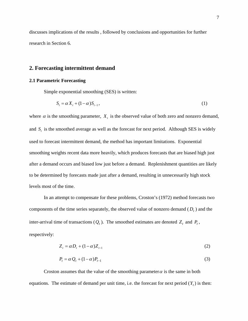

8
ttt PZY (4)
If there is no demand in a period and are unchanged Note that when demand
occurs every period the Croston method gives the same forecasts as conventional SES Thus the
same method can be used for both intermittent and non-intermittent demands
tZ tP
Syntetos and Boylan (2001) show that is biased to over-forecast Later Syntetos and
Boylan (2005) developed the SBA method (for Syntetos-Boylan Approximation) a modified
version of equation (4) that is approximately unbiased
tY
))(21( ttt PZY (5)
SES Croston and SBA are used below to forecast demand over the lead time plus review
period As recommended by Syntetos and Boylan (2006) on the grounds of simplicity the
variance of the forecast errors is estimated by the exponentially smoothed mean squared error
(MSE) over the lead time plus review period
22 Non-Parametric Forecasting
Non-parametric or bootstrapping approaches to forecasting permit a reconstruction of the
empirical distribution of the data thus making distributional assumptions redundant
Bootstrapping works by taking many random samples from a larger sample or from a population
itself These samples may be different from each other and from the population and they are
used to build up a histogram of the distribution of inventory demands during lead time
Statistics such as the mean and variance of lead-time demand are computed directly from the
histogram rather than inferred from a theoretical distribution
The WSS method is an advanced form of bootstrapping that captures the autocorrelation
between demand realizations and can produce values that have not appeared in the history The
9
method estimates transition probabilities in a two-state (zero vs non-zero) Markov model and
uses that model to generate a sequence of zero and non-zero demand occurrences The non-zero
occurrences are then assigned a positive value (demand) by using an ad-hoc method of ldquojitteringrdquo
proposed by the authors The WSS method works according to the following steps which are
found in both WSS (2004) and Willemain and Smart (2001)
1 Obtain historical demand data in chosen time buckets (eg days weeks months) 2 Estimate transition probabilities for a two-state (zero vs non-zero) Markov model 3 Conditional on last observed demand use the Markov model to generate a sequence of
zeronon-zero values over the forecast horizon (lead time) 4 Replace every non-zero state marker with a numerical value sampled at random with
replacement from the set of observed non-zero demands 5 ldquoJitterrdquo the non-zero demand values X When X is selected at random generate a
realization of a standard normal random deviate Z The jittered value is )INT(1 X Z X unless the result is less than or equal to zero in which case the
jittered value is simply X 6 Sum the forecast values over the horizon to get one predicted value of lead time demand
(LTD)
Porras and Dekker (2008) propose an empirical method based on the construction of a
histogram of demands over the lead time (L) A block of L consecutive demand observations is
sampled repeatedly with replacement Such a procedure results in capturing the potential auto-
correlation of the demand data The method is intuitively appealing and links naturally to stock
control However the method cannot extrapolate beyond previous demands (an important
advantage of WSS) making it difficult to attain realistically high service level targets
10
Preliminary results not reported here show poor performance of the Porras and Decker method
which is not considered further
Viswanathan and Zhou (2008) claim an improvement to the WSS bootstrapping
procedure The key difference is that instead of the two-state Markov chain used by WSS the
historical inter-demand interval distribution generates demand arrivals However this procedure
is heavily dependent upon lengthy demand histories that are not often available Zhou and
Viswanathan (2011) compare their procedure to parametric methods on empirical data and find
the parametric methods are more accurate They attribute the inferior performance of the
bootstrapping method to the short demand histories available and this approach is not considered
further
Finally a parametric bootstrapping method proposed by Snyder (2002) was shown to
perform well on a few SKUs However we did not consider the Snyder method due to its
constraining theoretical assumptions that defy the purpose of using bootstrapping procedures in
the first place
3 Experimental design
31 Data
Forecasting performance is tested in the data described in Tables 1 ndash 2 (all data are
available from the corresponding author) The jewelry data are one year of weekly retail
demands for an inexpensive line of costume jewelry the distribution of demand intervals is
relatively compact around a median of 44 weeks and most demands are for one or two units
Stock replenishment lead-times in the jewelry data are one week A Japanese manufacturer
supplied the electronics data which consists of four years of monthly demand histories for spare
11
parts used in European support operations The median demand interval is relatively short at 26
months but both demand intervals and sizes are skewed right due to outliers in most time series
Lead-times in the electronics data are three months which makes stock control far more difficult
than in the jewelry data
------------------------------
Insert Table 1 Here ------------------------------
------------------------------ Insert Table 2 Here
------------------------------
32 Performance Measurement
Syntetos and Boylan (2006) and Syntetos Nikolopoulos and Boylan (2010) demonstrate
that there is little relationship between traditional measures of forecast accuracy such as the
mean error and stock control performance as measured by inventory investment and customer
service (For a general discussion of the organizational and inventory implications of forecast
errors refer to Sanders amp Graman 2009) Therefore accuracy measures are bypassed in this
study and forecasting is evaluated by its direct effects on stock control Gardner (1990 2006)
recommends the use of tradeoff curves for this purpose and that example is followed here by
computing tradeoffs between total inventory investment and customer service
Another suggestion for evaluating performance is the use of average regret metrics (Sani
and Kingsman 1997) or implied stock-holdings that are based on a calculation of the exact
safety margin providing a maximum stock-out of zero (Eaves and Kingsman 2004) An
alternative formulation involves fixing a target service measure and searching for the investment
necessary to hit the target However tradeoff curves are the most realistic representation of the
12
various methodsrsquo comparative performance and the most meaningful one from a practitioner
perspective
Performance is simulated using a periodic order-up-to-level stock control system which
is widely used in practice because it requires optimization of only one parameter the order-up-
to-level The stock control system is designed to meet a target fraction of replenishment cycles
in which total demand can be delivered from stock This fraction is called the cycle service level
(CSL) (ie the probability of no stock-outs during a replenishment cycle) During out-of-sample
testing the forecasting methods are used to compute weekly or monthly order-up-to-levels that
attempt to meet four CSL targets 85 90 95 and 99 Other service measures (like the
most commonly used fill rate for example) are not considered because bootstrapping does not
allow direct calculation of such measures
For the parametric methods the order-up-to-level in each period is computed as the
inverse of the cumulative distribution function of demand over the lead time plus one review
period Replenishment decisions take place at the end of every period (week or month) so the
review period is set equal to one Demands are assumed to follow the Negative Binomial
Distribution (NBD) One difficulty with the NBD is that it requires the variance to be greater
than the mean in the few cases where the reverse was true the variance is set equal to 11 times
the mean Although this may look ad hoc Sani (1995) shows that it produces robust results
33 Model-Fitting and Forecasting
To test the parametric forecasting methods the demand history for each SKU is split into
two parts within sample (for initialization and optimization purposes) and out-of-sample (for
reporting performance) The first 12 observations are used as an initialization sample to compute
13
an average for the beginning level of demand and in the case of Crostonrsquos method the beginning
demand size and interval (expressed also as averages of the corresponding variables over the
initialization block) To make the most use of the data available the optimization block contains
the initialization block and extends it by the same number of periods That is the first 24
observations are used as an optimization sample to select the smoothing parameter over the range
005 to 030 (in steps of 001) that minimizes the mean squared error (MSE) per series (For more
details on the issue of optimization of parameters in an intermittent demand context please refer
to Petropoulos Nikolopoulos Spithourakis amp Assimakopoulos 2013) Variances are estimated
by the cumulative smoothed MSE using a fixed smoothing parameter of 025 analysis not
reported here indicates that this value performs well In Crostonrsquos original method the same
smoothing parameter updates both demand size and interval but a separate smoothing parameter
for each one is used here following Schultzrsquos (1987) advice that separate parameters lead to
better forecast accuracy For the WSS method the within sample data are used to compute an
initial value for the order-up-to-level which is then updated weekly or monthly Out-of-sample
testing starts at period 25 so there are 28 out-of-sample observations in each jewelry series and
24 in each electronics series
4 Empirical results
Three performance measures are reported for every combination of forecasting method
dataset and target CSL First total inventory investment is computed by pricing each SKU by
unit cost and summing across all SKUs Second the achieved CSL is computed as the actual
percentage of replenishment cycles in which demand is satisfied directly from stock on hand
Finally total backorders are computed by averaging backorder values over time (weeks or
14
months) for each SKU and then summing across all SKUs These measures are presented in the
form of tradeoff curves showing achieved CSL and total backorders as a function of total
investment Each curve has four plotting symbols corresponding to the four CSL targets
41 Jewelry Data
In the jewelry data Figure 1 shows tradeoff curves between investment and CSL All
forecasting methods achieve CSLs slightly larger than the 99 target (with the exception of SES
that just falls short of that) but achieved levels are significantly greater than targets of 85
90 and 95 The descriptive statistics presented in Table 2 indicate that the jewelry data are
neither particularly intermittent nor erratic the latter referring to the variability of the demand
sizes Thus the NBD provides a good fit to the empirical data and the parametric methods
produce very similar CSL tradeoff curves (with the SBA and Croston being indicated as the
lsquobestrsquo approaches) The curve for the WSS method runs above the parametric curves at targets
of 95 and 99 and gives a slightly better CSL for any level of investment greater than about
$130000 For example at an investment of $175000 WSS adds about one percentage point to
CSL compared to the other methods Inventory investment vs backorders are plotted in Figure 2
and again the parametric methods produce similar results while the WSS method yields lower
backorder values for any investment greater than $130000
------------------------------ Insert Figure 1 Here
------------------------------
------------------------------ Insert Figure 2 Here
------------------------------
15
42 Electronics Data
The electronics data are more erratic than the jewelry data and the results are
considerably different In Figure 3 all methods achieve CSLs greater than the 85 target and
all methods are close to the 90 target However at the 95 and 99 target all methods
significantly underperform For example when SES is run with a target of 99 the achieved
CSL is only 95 Outliers in the electronics data make it extremely difficult to estimate the
parameters of the demand distribution and hit the CSL targets
The Croston method consistently gives better CSL performance than the SBA method
even though SBA was designed to improve on Croston The problem is that the Croston method
is biased high which increases both customer service and inventory investment SES produces
the best CSL tradeoff curve through an investment of about euro48 million and thereafter WSS is
marginally better At an investment of euro40 million SES yields a CSL about one percentage
point better than WSS But at an investment of euro65 million WSS is about one-half percentage
point better than SES
Differences in backorder performance are more significant In Figure 4 all parametric
methods produce smaller backorders than WSS at all levels of investment For example at an
investment of euro35 million SES backorders are euro14 million compared to euro22 million for WSS
SES yields the smallest backorders though an investment of about euro50 million thereafter the
SBA method is best followed closely by Croston
------------------------------ Insert Figure 3 Here
------------------------------
------------------------------ Insert Figure 4 Here
------------------------------
16
5 Implications and practical considerations
The jewelry data are relatively well behaved with moderately intermittent demands and
short lead times all parametric methods give similar performance and the WSS bootstrapping
method is marginally better than the parametric methods The electronics data are more difficult
to forecast because they are more intermittent contain more outliers and have longer lead times
Under these conditions we might expect WSS to perform better than the parametric methods
but this did not happen In the electronics data all parametric methods give significantly better
backorder performance than WSS
Willemain et al (2004) claimed that an important advantage related to the use of
bootstrapping is its attractiveness to practitioners ldquoUsers intuitively grasp the simple
procedural explanation of how the bootstrap works Their comfort with the bootstrap approach
may derive from the concrete algorithmic nature of computational inference in contrast to the
more abstract character of traditional mathematical approaches to statistical inferencerdquo This
claim may be true for the general bootstrapping concept but the details of the WSS method such
as the use of transition probabilities and Markov models are more complicated and difficult to
understand than any of the parametric methods tested
Another consideration in evaluating the WSS procedure is that demand forecasts are
often subject to judgmental adjustments (Syntetos Nikolopoulos Boylan Fildes amp Goodwin
2009) Such adjustments can be beneficial especially when they are based on information not
available to the forecasting model However adjustments can be unnecessary or even harmful
when they are applied without an understanding of how the forecasts were produced Simple
methods should result in fewer damaging judgmental interventions
17
Although the parametric forecasting methods are simple their interactions with stock
control are not Many authors have pointed out that forecast errors may seriously distort
projections of customer service levels in an intermittent demand context The fundamental
problem is that inventory theory has been developed upon the assumptions of known moments of
the hypothesized demand distribution Although no concrete theory has been developed in this
area there is an expectation that parametric estimators will sometimes under-achieve the
specified targets A common reaction from practitioners is to incorporate some bias in the
forecasts to avoid running out of stock However such adjustments are not straightforward since
the variance of the estimates (sampling error of the mean) is also affected leading to confusion
about the effects on performance of the system
The application of bootstrapping is relatively straightforward under the CSL constraint
but such is not the case should other service measures and cost criteria be considered Parametric
theory despite its shortcomings does provide guidelines for optimization of the stock control
system under a wide range of objectives andor constraints More research is needed to extend
the capacity of bootstrapping to match parametric theory Consider for example the specification
of a fill-rate target as opposed to the CSL in a practical setting bootstrapping cannot be used
directly to meet a fill-rate target
6 Conclusions and future research
The WSS method of bootstrapping does have advantages most notably the ability to
simulate demand values that have not appeared in history However it is questionable whether
the WSS method is worth the considerable added complexity Parametric methods are simpler
18
and the simplest method of all SES performs well In the messy electronics data SES produces
fewer backorders than WSS at all levels of inventory investment
Parametric methods require less computing power which is important when demands for
very large numbers of SKUs have to be forecast Parametric methods also require less specialist
knowledge and thus are more transparent and more resistant to potentially damaging judgmental
interventions
Teunter and Duncan (2009) observed that analytical projections of customer service are
often different from empirical results in an intermittent demand context a conclusion that applies
to this study as well In the jewelry data achieved CSLs for all methods were significantly
greater than targets of 85 90 and 95 In the electronics data achieved CSLs were
significantly less than targets of 95 and 99 The difference between target and achieved
CSLs are attributed to errors in estimating the parameters of the demand distribution if these
parameters were known achieved CSLs should correspond to the targets
There are several opportunities for further research in intermittent demand forecasting
The M and M3 forecasting competitions (Makridakis Andersen Carbone Fildes Hibon
Lewandowski Newton Parzen amp Winkler 1982 and Makridakis amp Hibon 2000 respectively)
did not consider intermittent demand data Future competitions should include such data
An alternative strategy to deal with intermittent demand patterns is to aggregate demand
in lower-frequency time buckets thereby reducing the presence of zero observations Temporal
aggregation is a practice employed in many real world settings but there has been no research
apart from a few studies (Nikolopoulos Syntetos Boylan Petropoulos amp Assimakopoulos
2011 Babai Ali amp Nikolopoulos 2012 Spithourakis Petropoulos Nikolopoulos amp
Assimakopoulos 2012)
19
Another research opportunity is to consider stationary models for intermittent demand
forecasting rather than restricting attention to models based on Crostonrsquos method For example
Poisson autoregressive models have been suggested by Shenstone and Hyndman (2005) Models
based on a variety of count probability distributions coupled with dynamic specifications to
account for potential serial correlation have recently been analyzed by Snyder et al (2012)
although the authors made no attempt to evaluate stock control results Further development and
testing of such models in the context of stock control is the next step in our research
Finally we acknowledge that the bootstrapping algorithm considered in this paper is the
exclusive property of Smart Software Inc under US Patent 6205431 B1 Use in this paper was
permitted by a special licensing arrangement with Smart Software and does not imply a public
license to use the algorithm According to Smart Software ldquoThis algorithm differs in several
important ways from the commercial implementation in the SmartForecaststrade software so
conclusions about the performance of the algorithm implemented here cannot be extrapolated to
the performance of SmartForecaststrade Further Smart Software provided no oversight or
guidance in implementing the algorithmrdquo
Note At least one of the authors has read each reference in this paper We contacted
Ruud Teunter and Thomas Willemain to ensure that their work was properly summarized
References
Babai MZ Ali M amp Nikolopoulos K (2012) Impact of temporal aggregation on stock
control performance of intermittent demand estimators OMEGA international Journal of
Management Science 40(6) 713-721
20
Boylan JE amp Syntetos AA (2008) Forecasting for inventory management of service parts In
DNP Murthy amp KAH Kobbacy (Eds) Complex system maintenance handbook London
Springer Verlag 479-508
Brown RG (1959) Statistical forecasting for inventory control New York McGraw-Hill
Cattani KD Jacobs FR amp Schoenfelder J (2011) Common inventory modelling assumptions
that fall short Arborescent networks Poisson demand and single echelon approximations Journal of
Operations Management 29(5) 488-499
Croston JD (1972) Forecasting and stock control for intermittent demands Operational
Research Quarterly 23(3) 289-304
Deloitte (2011) The service revolution in global manufacturing industries New York Deloitte
Research
Dunsmuir WTM amp Snyder RD (1989) Control of inventories with intermittent demand
European Journal of Operational Research 40(1) 16-21
Eaves AHC (2002) Forecasting for the ordering and stock holding of consumable spare
parts Doctoral dissertation Lancaster University Lancaster UK
21
Eaves AHC amp Kingsman BG (2004) Forecasting for the ordering and stockholding of spare
parts Journal of the Operational Research Society 55(4) 431-437
Efron B (1979) Bootstrap methods another look at the jackknife Annals of Statistics 7(1) 1-
26
Gardner ES (1990) Evaluating forecast performance in an inventory control system
Management Science 36(4) 490-499
Gardner ES (2006) Exponential smoothing the state of the art - part II International Journal
of Forecasting 22(4) 637ndash666
Gardner ES amp Koehler AB (2005) Comments on a patented bootstrapping method for
forecasting intermittent demand International Journal of Forecasting 21(3) 617-618
Gutierrez RS Solis AO amp Mukhopadhyay S (2008) Lumpy demand forecasting using
neural networks International Journal of Production Economics 111(2) 409-420
Hinton Jr HL (1999) Defense inventory continuing challenges in managing inventories and
avoiding adverse operational effects Washington DC US General Accounting Office
22
Janssen FBSLP (1998) Inventory management systems control and information issues
Doctoral dissertation Centre for Economic Research Tilburg University Tilburg The
Netherlands
Johnston F R amp Boylan J E (1996) Forecasting for items with intermittent demand Journal
of the Operational Research Society 47(1) 113ndash121
Johnston FR Boylan JE amp Shale EA (2003) An examination of the size of orders from
customers their characterization and the implications for inventory control of slow moving
items Journal of the Operational Research Society 54(8) 833-837
Makridakis S Andersen A Carbone R Fildes R Hibon M Lewandowski R Newton J
Parzen E amp Winkler R (1982) The accuracy of extrapolation (time series) methods results of
a forecasting competition Journal of Forecasting 1(2) 111-153
Makridakis S amp Hibon M (2000) The M3-competition results conclusions and implications
International Journal of Forecasting 16(4) 451-476
Molenaers A Baets H Pintelon L amp Waeyenberg G (2010) Criticality classification of
spare parts A case study Preprints of the 16th International Working Seminar on Production
Economics Innsbruck Austria
23
Nikolopoulos K Syntetos AA Boylan JE Petropoulos F amp Assimakopoulos V (2011) An
aggregate ndash disaggregate intermittent demand approach (ADIDA) to forecasting An empirical
proposition and analysis Journal of the Operational Research Society 62(3) 544-554
Petropoulos F Nikolopoulos K Spithourakis GP amp Assimakopoulos V (2013) Empirical
heuristics for improving intermittent demand forecasting Industrial Management amp Data
Systems 113(5) 683-696
Porras EM amp Dekker R (2008) An inventory control system for spare parts at a refinery An
empirical comparison of different reorder point methods European Journal of Operational
Research 184(1) 101-132
Rao A V (1973) A comment on Forecasting and stock control for intermittent demands
Operational Research Quarterly 24(4) 639-640
Sanders NR amp Graman GA (2009) Quantifying costs of forecast errors A case study of the
warehouse environment OMEGA The International Journal of Management Science 37(1)
116-125
Sani B (1995) Periodic inventory control systems and demand forecasting methods for low
demand items Doctoral dissertation Lancaster University Lancaster UK
24
Sani B amp Kingsman BG (1997) Selecting the best periodic inventory control and demand
forecasting methods for low demand items Journal of the Operational Research Society 48 (7)
700-713
Schultz CR (1987) Forecasting and inventory control for sporadic demand under periodic
review Journal of the Operational Research Society 38(5) 453-458
Shale EA Boylan JE amp Johnston FR (2006) Forecasting for intermittent demand the
estimation of an unbiased average Journal of the Operational Research Society 57(5) 588-592
Shenstone L amp Hyndman RJ (2005) Stochastic models underlying Crostonrsquos method for
intermittent demand forecasting Journal of Forecasting 24(6) 389-402
Snyder R (2002) Forecasting sales of slow and fast moving inventories European Journal of
Operational Research 140(3) 684-699
Snyder R Ord K amp Beaumont A (2012) Forecasting the intermittent demand for slow-
moving inventories a modelling approach International Journal of Forecasting 28(2) 485-496
Spithourakis GP Petropoulos F Nikolopoulos K amp Assimakopoulos V (2012) A systemic
view of the ADIDA framework IMA Journal of Management Mathematics advance online
publication doi101093imamandps031
25
Syntetos AA amp Boylan JE (2001) On the bias of intermittent demand estimates
International Journal of Production Economics 71(1-3) 457-466
Syntetos AA amp Boylan JE (2005) The Accuracy of Intermittent Demand Estimates
International Journal of Forecasting 21(2) 303-314
Syntetos AA amp Boylan JE (2006) On the stock control performance of intermittent demand
estimators International Journal of Production Economics 103(1) 36-47
Syntetos AA Keyes M amp Babai MZ (2009) Demand categorisation in a European spare
parts logistics network International Journal of Operations and Production Management 29(3)
292-316
Syntetos AA Nikolopoulos K Boylan JE Fildes R amp Goodwin P (2009) The ffects of
integrating management judgement into intermittent demand forecasts International Journal of
Production Economics 118(1) 72-81
Syntetos AA Nikolopoulos K amp Boylan JE (2010) Judging the judges through accuracy-
implication metrics The case of inventory forecasting International Journal of Forecasting 26(1)
134-143
26
Teunter R amp Duncan L (2009) Forecasting intermittent demand A comparative study
Journal of the Operational Research Society 60(3) 321-329
Teunter R Syntetos AA amp Babai MZ (2011) Intermittent demand Linking forecasting to
inventory obsolescence European Journal of Operational Research 214(3) 606-615
Viswanathan S amp Zhou CX (2008) A new bootstrapping based method for forecasting and
safety stock determination for intermittent demand items Working paper Nanyang Business
School Nanyang Technological University Singapore
Willemain TR amp Smart CN (2001) United States Patent 6205431 B1 System and method
for forecasting intermittent demand Available at httppatftusptogov
Willemain TR Smart CN Shockor JH amp DeSautels PA (1994) Forecasting intermittent
demand in manufacturing A comparative evaluation of Crostonrsquos method International Journal
of Forecasting 10(4) 529-538
Willemain TR Smart CN amp Schwarz HF (2004) A new approach to forecasting
intermittent demand for service parts inventories International Journal of Forecasting 20(3)
375-387
27
Willemain TR Smart CN amp Schwarz HF (2005) Authorrsquos response to Koehler and
Gardner International Journal of Forecasting 21(3) 619-620
Zhou CX amp Viswanathan S (2011) Comparison of a new bootstrapping method with
parametric approaches for safety stock determination in service parts inventory systems
International Journal of Production Economics 133(1) 481-485
28
TABLES
Table 1 Jewelry data - 52 weeks of demands for 4076 SKUs
Mean Std Dev Mean Std Dev Mean Std DevMinimum 13 06 10 00 01 0325th percentile 33 26 11 03 02 04Median 44 37 12 04 03 0575th percentile 56 50 14 07 04 07Maximum 87 130 32 37 22 25
Demand interval Demand size Demand per period
Table 2 Electronics data - 48 months of demands for 3055 SKUs
Mean Std Dev Mean Std Dev Mean Std DevMinimum 10 00 10 00 00 0225th percentile 15 10 35 30 09 22Median 26 23 59 62 21 4575th percentile 47 44 121 139 60 105Maximum 240 325 53662 91493 53662 38584
Demand interval Demand size Demand per period
29
FIGURES
Figure 1 Jewelry data - investment vs CSL
88
90
92
94
96
98
100
50 100 150 200 250 300
Inventory investment (K$)
Ach
ieve
d C
SL
SES
Croston
SBA
WSS
Figure 2 Jewelry data - investment vs backorders
0
2
4
6
8
10
12
50 100 150 200 250 300
Inventory investment (K$)
Bac
kord
ers
(K$)
SES
Croston
SBA
WSS
30
Figure 3 Electronics data - investment vs CSL
84
86
88
90
92
94
96
98
30 35 40 45 50 55 60 65 70 75 80
Inventory investment (Meuro)
Ach
ieve
d C
SL
SES
Croston
SBA
WSS
Figure 4 Electronics data - investment vs backorders
00
05
10
15
20
25
30 35 40 45 50 55 60 65 70 75 80
Inventory investment (Meuro)
Bac
kord
ers
(Meuro)
SES
Croston
SBA
WSS
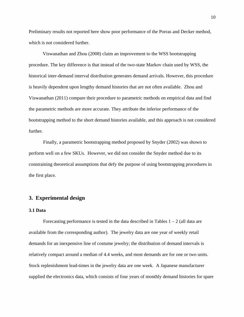
10
Preliminary results not reported here show poor performance of the Porras and Decker method
which is not considered further
Viswanathan and Zhou (2008) claim an improvement to the WSS bootstrapping
procedure The key difference is that instead of the two-state Markov chain used by WSS the
historical inter-demand interval distribution generates demand arrivals However this procedure
is heavily dependent upon lengthy demand histories that are not often available Zhou and
Viswanathan (2011) compare their procedure to parametric methods on empirical data and find
the parametric methods are more accurate They attribute the inferior performance of the
bootstrapping method to the short demand histories available and this approach is not considered
further
Finally a parametric bootstrapping method proposed by Snyder (2002) was shown to
perform well on a few SKUs However we did not consider the Snyder method due to its
constraining theoretical assumptions that defy the purpose of using bootstrapping procedures in
the first place
3 Experimental design
31 Data
Forecasting performance is tested in the data described in Tables 1 ndash 2 (all data are
available from the corresponding author) The jewelry data are one year of weekly retail
demands for an inexpensive line of costume jewelry the distribution of demand intervals is
relatively compact around a median of 44 weeks and most demands are for one or two units
Stock replenishment lead-times in the jewelry data are one week A Japanese manufacturer
supplied the electronics data which consists of four years of monthly demand histories for spare
11
parts used in European support operations The median demand interval is relatively short at 26
months but both demand intervals and sizes are skewed right due to outliers in most time series
Lead-times in the electronics data are three months which makes stock control far more difficult
than in the jewelry data
------------------------------
Insert Table 1 Here ------------------------------
------------------------------ Insert Table 2 Here
------------------------------
32 Performance Measurement
Syntetos and Boylan (2006) and Syntetos Nikolopoulos and Boylan (2010) demonstrate
that there is little relationship between traditional measures of forecast accuracy such as the
mean error and stock control performance as measured by inventory investment and customer
service (For a general discussion of the organizational and inventory implications of forecast
errors refer to Sanders amp Graman 2009) Therefore accuracy measures are bypassed in this
study and forecasting is evaluated by its direct effects on stock control Gardner (1990 2006)
recommends the use of tradeoff curves for this purpose and that example is followed here by
computing tradeoffs between total inventory investment and customer service
Another suggestion for evaluating performance is the use of average regret metrics (Sani
and Kingsman 1997) or implied stock-holdings that are based on a calculation of the exact
safety margin providing a maximum stock-out of zero (Eaves and Kingsman 2004) An
alternative formulation involves fixing a target service measure and searching for the investment
necessary to hit the target However tradeoff curves are the most realistic representation of the
12
various methodsrsquo comparative performance and the most meaningful one from a practitioner
perspective
Performance is simulated using a periodic order-up-to-level stock control system which
is widely used in practice because it requires optimization of only one parameter the order-up-
to-level The stock control system is designed to meet a target fraction of replenishment cycles
in which total demand can be delivered from stock This fraction is called the cycle service level
(CSL) (ie the probability of no stock-outs during a replenishment cycle) During out-of-sample
testing the forecasting methods are used to compute weekly or monthly order-up-to-levels that
attempt to meet four CSL targets 85 90 95 and 99 Other service measures (like the
most commonly used fill rate for example) are not considered because bootstrapping does not
allow direct calculation of such measures
For the parametric methods the order-up-to-level in each period is computed as the
inverse of the cumulative distribution function of demand over the lead time plus one review
period Replenishment decisions take place at the end of every period (week or month) so the
review period is set equal to one Demands are assumed to follow the Negative Binomial
Distribution (NBD) One difficulty with the NBD is that it requires the variance to be greater
than the mean in the few cases where the reverse was true the variance is set equal to 11 times
the mean Although this may look ad hoc Sani (1995) shows that it produces robust results
33 Model-Fitting and Forecasting
To test the parametric forecasting methods the demand history for each SKU is split into
two parts within sample (for initialization and optimization purposes) and out-of-sample (for
reporting performance) The first 12 observations are used as an initialization sample to compute
13
an average for the beginning level of demand and in the case of Crostonrsquos method the beginning
demand size and interval (expressed also as averages of the corresponding variables over the
initialization block) To make the most use of the data available the optimization block contains
the initialization block and extends it by the same number of periods That is the first 24
observations are used as an optimization sample to select the smoothing parameter over the range
005 to 030 (in steps of 001) that minimizes the mean squared error (MSE) per series (For more
details on the issue of optimization of parameters in an intermittent demand context please refer
to Petropoulos Nikolopoulos Spithourakis amp Assimakopoulos 2013) Variances are estimated
by the cumulative smoothed MSE using a fixed smoothing parameter of 025 analysis not
reported here indicates that this value performs well In Crostonrsquos original method the same
smoothing parameter updates both demand size and interval but a separate smoothing parameter
for each one is used here following Schultzrsquos (1987) advice that separate parameters lead to
better forecast accuracy For the WSS method the within sample data are used to compute an
initial value for the order-up-to-level which is then updated weekly or monthly Out-of-sample
testing starts at period 25 so there are 28 out-of-sample observations in each jewelry series and
24 in each electronics series
4 Empirical results
Three performance measures are reported for every combination of forecasting method
dataset and target CSL First total inventory investment is computed by pricing each SKU by
unit cost and summing across all SKUs Second the achieved CSL is computed as the actual
percentage of replenishment cycles in which demand is satisfied directly from stock on hand
Finally total backorders are computed by averaging backorder values over time (weeks or
14
months) for each SKU and then summing across all SKUs These measures are presented in the
form of tradeoff curves showing achieved CSL and total backorders as a function of total
investment Each curve has four plotting symbols corresponding to the four CSL targets
41 Jewelry Data
In the jewelry data Figure 1 shows tradeoff curves between investment and CSL All
forecasting methods achieve CSLs slightly larger than the 99 target (with the exception of SES
that just falls short of that) but achieved levels are significantly greater than targets of 85
90 and 95 The descriptive statistics presented in Table 2 indicate that the jewelry data are
neither particularly intermittent nor erratic the latter referring to the variability of the demand
sizes Thus the NBD provides a good fit to the empirical data and the parametric methods
produce very similar CSL tradeoff curves (with the SBA and Croston being indicated as the
lsquobestrsquo approaches) The curve for the WSS method runs above the parametric curves at targets
of 95 and 99 and gives a slightly better CSL for any level of investment greater than about
$130000 For example at an investment of $175000 WSS adds about one percentage point to
CSL compared to the other methods Inventory investment vs backorders are plotted in Figure 2
and again the parametric methods produce similar results while the WSS method yields lower
backorder values for any investment greater than $130000
------------------------------ Insert Figure 1 Here
------------------------------
------------------------------ Insert Figure 2 Here
------------------------------
15
42 Electronics Data
The electronics data are more erratic than the jewelry data and the results are
considerably different In Figure 3 all methods achieve CSLs greater than the 85 target and
all methods are close to the 90 target However at the 95 and 99 target all methods
significantly underperform For example when SES is run with a target of 99 the achieved
CSL is only 95 Outliers in the electronics data make it extremely difficult to estimate the
parameters of the demand distribution and hit the CSL targets
The Croston method consistently gives better CSL performance than the SBA method
even though SBA was designed to improve on Croston The problem is that the Croston method
is biased high which increases both customer service and inventory investment SES produces
the best CSL tradeoff curve through an investment of about euro48 million and thereafter WSS is
marginally better At an investment of euro40 million SES yields a CSL about one percentage
point better than WSS But at an investment of euro65 million WSS is about one-half percentage
point better than SES
Differences in backorder performance are more significant In Figure 4 all parametric
methods produce smaller backorders than WSS at all levels of investment For example at an
investment of euro35 million SES backorders are euro14 million compared to euro22 million for WSS
SES yields the smallest backorders though an investment of about euro50 million thereafter the
SBA method is best followed closely by Croston
------------------------------ Insert Figure 3 Here
------------------------------
------------------------------ Insert Figure 4 Here
------------------------------
16
5 Implications and practical considerations
The jewelry data are relatively well behaved with moderately intermittent demands and
short lead times all parametric methods give similar performance and the WSS bootstrapping
method is marginally better than the parametric methods The electronics data are more difficult
to forecast because they are more intermittent contain more outliers and have longer lead times
Under these conditions we might expect WSS to perform better than the parametric methods
but this did not happen In the electronics data all parametric methods give significantly better
backorder performance than WSS
Willemain et al (2004) claimed that an important advantage related to the use of
bootstrapping is its attractiveness to practitioners ldquoUsers intuitively grasp the simple
procedural explanation of how the bootstrap works Their comfort with the bootstrap approach
may derive from the concrete algorithmic nature of computational inference in contrast to the
more abstract character of traditional mathematical approaches to statistical inferencerdquo This
claim may be true for the general bootstrapping concept but the details of the WSS method such
as the use of transition probabilities and Markov models are more complicated and difficult to
understand than any of the parametric methods tested
Another consideration in evaluating the WSS procedure is that demand forecasts are
often subject to judgmental adjustments (Syntetos Nikolopoulos Boylan Fildes amp Goodwin
2009) Such adjustments can be beneficial especially when they are based on information not
available to the forecasting model However adjustments can be unnecessary or even harmful
when they are applied without an understanding of how the forecasts were produced Simple
methods should result in fewer damaging judgmental interventions
17
Although the parametric forecasting methods are simple their interactions with stock
control are not Many authors have pointed out that forecast errors may seriously distort
projections of customer service levels in an intermittent demand context The fundamental
problem is that inventory theory has been developed upon the assumptions of known moments of
the hypothesized demand distribution Although no concrete theory has been developed in this
area there is an expectation that parametric estimators will sometimes under-achieve the
specified targets A common reaction from practitioners is to incorporate some bias in the
forecasts to avoid running out of stock However such adjustments are not straightforward since
the variance of the estimates (sampling error of the mean) is also affected leading to confusion
about the effects on performance of the system
The application of bootstrapping is relatively straightforward under the CSL constraint
but such is not the case should other service measures and cost criteria be considered Parametric
theory despite its shortcomings does provide guidelines for optimization of the stock control
system under a wide range of objectives andor constraints More research is needed to extend
the capacity of bootstrapping to match parametric theory Consider for example the specification
of a fill-rate target as opposed to the CSL in a practical setting bootstrapping cannot be used
directly to meet a fill-rate target
6 Conclusions and future research
The WSS method of bootstrapping does have advantages most notably the ability to
simulate demand values that have not appeared in history However it is questionable whether
the WSS method is worth the considerable added complexity Parametric methods are simpler
18
and the simplest method of all SES performs well In the messy electronics data SES produces
fewer backorders than WSS at all levels of inventory investment
Parametric methods require less computing power which is important when demands for
very large numbers of SKUs have to be forecast Parametric methods also require less specialist
knowledge and thus are more transparent and more resistant to potentially damaging judgmental
interventions
Teunter and Duncan (2009) observed that analytical projections of customer service are
often different from empirical results in an intermittent demand context a conclusion that applies
to this study as well In the jewelry data achieved CSLs for all methods were significantly
greater than targets of 85 90 and 95 In the electronics data achieved CSLs were
significantly less than targets of 95 and 99 The difference between target and achieved
CSLs are attributed to errors in estimating the parameters of the demand distribution if these
parameters were known achieved CSLs should correspond to the targets
There are several opportunities for further research in intermittent demand forecasting
The M and M3 forecasting competitions (Makridakis Andersen Carbone Fildes Hibon
Lewandowski Newton Parzen amp Winkler 1982 and Makridakis amp Hibon 2000 respectively)
did not consider intermittent demand data Future competitions should include such data
An alternative strategy to deal with intermittent demand patterns is to aggregate demand
in lower-frequency time buckets thereby reducing the presence of zero observations Temporal
aggregation is a practice employed in many real world settings but there has been no research
apart from a few studies (Nikolopoulos Syntetos Boylan Petropoulos amp Assimakopoulos
2011 Babai Ali amp Nikolopoulos 2012 Spithourakis Petropoulos Nikolopoulos amp
Assimakopoulos 2012)
19
Another research opportunity is to consider stationary models for intermittent demand
forecasting rather than restricting attention to models based on Crostonrsquos method For example
Poisson autoregressive models have been suggested by Shenstone and Hyndman (2005) Models
based on a variety of count probability distributions coupled with dynamic specifications to
account for potential serial correlation have recently been analyzed by Snyder et al (2012)
although the authors made no attempt to evaluate stock control results Further development and
testing of such models in the context of stock control is the next step in our research
Finally we acknowledge that the bootstrapping algorithm considered in this paper is the
exclusive property of Smart Software Inc under US Patent 6205431 B1 Use in this paper was
permitted by a special licensing arrangement with Smart Software and does not imply a public
license to use the algorithm According to Smart Software ldquoThis algorithm differs in several
important ways from the commercial implementation in the SmartForecaststrade software so
conclusions about the performance of the algorithm implemented here cannot be extrapolated to
the performance of SmartForecaststrade Further Smart Software provided no oversight or
guidance in implementing the algorithmrdquo
Note At least one of the authors has read each reference in this paper We contacted
Ruud Teunter and Thomas Willemain to ensure that their work was properly summarized
References
Babai MZ Ali M amp Nikolopoulos K (2012) Impact of temporal aggregation on stock
control performance of intermittent demand estimators OMEGA international Journal of
Management Science 40(6) 713-721
20
Boylan JE amp Syntetos AA (2008) Forecasting for inventory management of service parts In
DNP Murthy amp KAH Kobbacy (Eds) Complex system maintenance handbook London
Springer Verlag 479-508
Brown RG (1959) Statistical forecasting for inventory control New York McGraw-Hill
Cattani KD Jacobs FR amp Schoenfelder J (2011) Common inventory modelling assumptions
that fall short Arborescent networks Poisson demand and single echelon approximations Journal of
Operations Management 29(5) 488-499
Croston JD (1972) Forecasting and stock control for intermittent demands Operational
Research Quarterly 23(3) 289-304
Deloitte (2011) The service revolution in global manufacturing industries New York Deloitte
Research
Dunsmuir WTM amp Snyder RD (1989) Control of inventories with intermittent demand
European Journal of Operational Research 40(1) 16-21
Eaves AHC (2002) Forecasting for the ordering and stock holding of consumable spare
parts Doctoral dissertation Lancaster University Lancaster UK
21
Eaves AHC amp Kingsman BG (2004) Forecasting for the ordering and stockholding of spare
parts Journal of the Operational Research Society 55(4) 431-437
Efron B (1979) Bootstrap methods another look at the jackknife Annals of Statistics 7(1) 1-
26
Gardner ES (1990) Evaluating forecast performance in an inventory control system
Management Science 36(4) 490-499
Gardner ES (2006) Exponential smoothing the state of the art - part II International Journal
of Forecasting 22(4) 637ndash666
Gardner ES amp Koehler AB (2005) Comments on a patented bootstrapping method for
forecasting intermittent demand International Journal of Forecasting 21(3) 617-618
Gutierrez RS Solis AO amp Mukhopadhyay S (2008) Lumpy demand forecasting using
neural networks International Journal of Production Economics 111(2) 409-420
Hinton Jr HL (1999) Defense inventory continuing challenges in managing inventories and
avoiding adverse operational effects Washington DC US General Accounting Office
22
Janssen FBSLP (1998) Inventory management systems control and information issues
Doctoral dissertation Centre for Economic Research Tilburg University Tilburg The
Netherlands
Johnston F R amp Boylan J E (1996) Forecasting for items with intermittent demand Journal
of the Operational Research Society 47(1) 113ndash121
Johnston FR Boylan JE amp Shale EA (2003) An examination of the size of orders from
customers their characterization and the implications for inventory control of slow moving
items Journal of the Operational Research Society 54(8) 833-837
Makridakis S Andersen A Carbone R Fildes R Hibon M Lewandowski R Newton J
Parzen E amp Winkler R (1982) The accuracy of extrapolation (time series) methods results of
a forecasting competition Journal of Forecasting 1(2) 111-153
Makridakis S amp Hibon M (2000) The M3-competition results conclusions and implications
International Journal of Forecasting 16(4) 451-476
Molenaers A Baets H Pintelon L amp Waeyenberg G (2010) Criticality classification of
spare parts A case study Preprints of the 16th International Working Seminar on Production
Economics Innsbruck Austria
23
Nikolopoulos K Syntetos AA Boylan JE Petropoulos F amp Assimakopoulos V (2011) An
aggregate ndash disaggregate intermittent demand approach (ADIDA) to forecasting An empirical
proposition and analysis Journal of the Operational Research Society 62(3) 544-554
Petropoulos F Nikolopoulos K Spithourakis GP amp Assimakopoulos V (2013) Empirical
heuristics for improving intermittent demand forecasting Industrial Management amp Data
Systems 113(5) 683-696
Porras EM amp Dekker R (2008) An inventory control system for spare parts at a refinery An
empirical comparison of different reorder point methods European Journal of Operational
Research 184(1) 101-132
Rao A V (1973) A comment on Forecasting and stock control for intermittent demands
Operational Research Quarterly 24(4) 639-640
Sanders NR amp Graman GA (2009) Quantifying costs of forecast errors A case study of the
warehouse environment OMEGA The International Journal of Management Science 37(1)
116-125
Sani B (1995) Periodic inventory control systems and demand forecasting methods for low
demand items Doctoral dissertation Lancaster University Lancaster UK
24
Sani B amp Kingsman BG (1997) Selecting the best periodic inventory control and demand
forecasting methods for low demand items Journal of the Operational Research Society 48 (7)
700-713
Schultz CR (1987) Forecasting and inventory control for sporadic demand under periodic
review Journal of the Operational Research Society 38(5) 453-458
Shale EA Boylan JE amp Johnston FR (2006) Forecasting for intermittent demand the
estimation of an unbiased average Journal of the Operational Research Society 57(5) 588-592
Shenstone L amp Hyndman RJ (2005) Stochastic models underlying Crostonrsquos method for
intermittent demand forecasting Journal of Forecasting 24(6) 389-402
Snyder R (2002) Forecasting sales of slow and fast moving inventories European Journal of
Operational Research 140(3) 684-699
Snyder R Ord K amp Beaumont A (2012) Forecasting the intermittent demand for slow-
moving inventories a modelling approach International Journal of Forecasting 28(2) 485-496
Spithourakis GP Petropoulos F Nikolopoulos K amp Assimakopoulos V (2012) A systemic
view of the ADIDA framework IMA Journal of Management Mathematics advance online
publication doi101093imamandps031
25
Syntetos AA amp Boylan JE (2001) On the bias of intermittent demand estimates
International Journal of Production Economics 71(1-3) 457-466
Syntetos AA amp Boylan JE (2005) The Accuracy of Intermittent Demand Estimates
International Journal of Forecasting 21(2) 303-314
Syntetos AA amp Boylan JE (2006) On the stock control performance of intermittent demand
estimators International Journal of Production Economics 103(1) 36-47
Syntetos AA Keyes M amp Babai MZ (2009) Demand categorisation in a European spare
parts logistics network International Journal of Operations and Production Management 29(3)
292-316
Syntetos AA Nikolopoulos K Boylan JE Fildes R amp Goodwin P (2009) The ffects of
integrating management judgement into intermittent demand forecasts International Journal of
Production Economics 118(1) 72-81
Syntetos AA Nikolopoulos K amp Boylan JE (2010) Judging the judges through accuracy-
implication metrics The case of inventory forecasting International Journal of Forecasting 26(1)
134-143
26
Teunter R amp Duncan L (2009) Forecasting intermittent demand A comparative study
Journal of the Operational Research Society 60(3) 321-329
Teunter R Syntetos AA amp Babai MZ (2011) Intermittent demand Linking forecasting to
inventory obsolescence European Journal of Operational Research 214(3) 606-615
Viswanathan S amp Zhou CX (2008) A new bootstrapping based method for forecasting and
safety stock determination for intermittent demand items Working paper Nanyang Business
School Nanyang Technological University Singapore
Willemain TR amp Smart CN (2001) United States Patent 6205431 B1 System and method
for forecasting intermittent demand Available at httppatftusptogov
Willemain TR Smart CN Shockor JH amp DeSautels PA (1994) Forecasting intermittent
demand in manufacturing A comparative evaluation of Crostonrsquos method International Journal
of Forecasting 10(4) 529-538
Willemain TR Smart CN amp Schwarz HF (2004) A new approach to forecasting
intermittent demand for service parts inventories International Journal of Forecasting 20(3)
375-387
27
Willemain TR Smart CN amp Schwarz HF (2005) Authorrsquos response to Koehler and
Gardner International Journal of Forecasting 21(3) 619-620
Zhou CX amp Viswanathan S (2011) Comparison of a new bootstrapping method with
parametric approaches for safety stock determination in service parts inventory systems
International Journal of Production Economics 133(1) 481-485
28
TABLES
Table 1 Jewelry data - 52 weeks of demands for 4076 SKUs
Mean Std Dev Mean Std Dev Mean Std DevMinimum 13 06 10 00 01 0325th percentile 33 26 11 03 02 04Median 44 37 12 04 03 0575th percentile 56 50 14 07 04 07Maximum 87 130 32 37 22 25
Demand interval Demand size Demand per period
Table 2 Electronics data - 48 months of demands for 3055 SKUs
Mean Std Dev Mean Std Dev Mean Std DevMinimum 10 00 10 00 00 0225th percentile 15 10 35 30 09 22Median 26 23 59 62 21 4575th percentile 47 44 121 139 60 105Maximum 240 325 53662 91493 53662 38584
Demand interval Demand size Demand per period
29
FIGURES
Figure 1 Jewelry data - investment vs CSL
88
90
92
94
96
98
100
50 100 150 200 250 300
Inventory investment (K$)
Ach
ieve
d C
SL
SES
Croston
SBA
WSS
Figure 2 Jewelry data - investment vs backorders
0
2
4
6
8
10
12
50 100 150 200 250 300
Inventory investment (K$)
Bac
kord
ers
(K$)
SES
Croston
SBA
WSS
30
Figure 3 Electronics data - investment vs CSL
84
86
88
90
92
94
96
98
30 35 40 45 50 55 60 65 70 75 80
Inventory investment (Meuro)
Ach
ieve
d C
SL
SES
Croston
SBA
WSS
Figure 4 Electronics data - investment vs backorders
00
05
10
15
20
25
30 35 40 45 50 55 60 65 70 75 80
Inventory investment (Meuro)
Bac
kord
ers
(Meuro)
SES
Croston
SBA
WSS
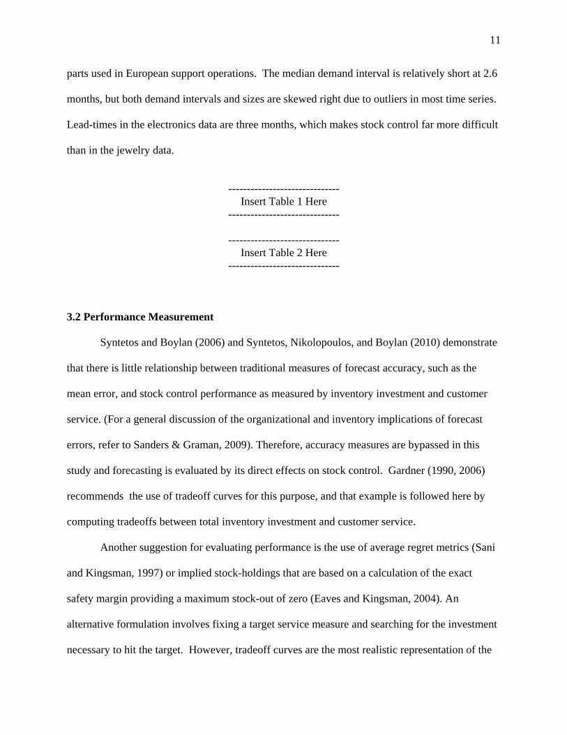

12
various methodsrsquo comparative performance and the most meaningful one from a practitioner
perspective
Performance is simulated using a periodic order-up-to-level stock control system which
is widely used in practice because it requires optimization of only one parameter the order-up-
to-level The stock control system is designed to meet a target fraction of replenishment cycles
in which total demand can be delivered from stock This fraction is called the cycle service level
(CSL) (ie the probability of no stock-outs during a replenishment cycle) During out-of-sample
testing the forecasting methods are used to compute weekly or monthly order-up-to-levels that
attempt to meet four CSL targets 85 90 95 and 99 Other service measures (like the
most commonly used fill rate for example) are not considered because bootstrapping does not
allow direct calculation of such measures
For the parametric methods the order-up-to-level in each period is computed as the
inverse of the cumulative distribution function of demand over the lead time plus one review
period Replenishment decisions take place at the end of every period (week or month) so the
review period is set equal to one Demands are assumed to follow the Negative Binomial
Distribution (NBD) One difficulty with the NBD is that it requires the variance to be greater
than the mean in the few cases where the reverse was true the variance is set equal to 11 times
the mean Although this may look ad hoc Sani (1995) shows that it produces robust results
33 Model-Fitting and Forecasting
To test the parametric forecasting methods the demand history for each SKU is split into
two parts within sample (for initialization and optimization purposes) and out-of-sample (for
reporting performance) The first 12 observations are used as an initialization sample to compute
13
an average for the beginning level of demand and in the case of Crostonrsquos method the beginning
demand size and interval (expressed also as averages of the corresponding variables over the
initialization block) To make the most use of the data available the optimization block contains
the initialization block and extends it by the same number of periods That is the first 24
observations are used as an optimization sample to select the smoothing parameter over the range
005 to 030 (in steps of 001) that minimizes the mean squared error (MSE) per series (For more
details on the issue of optimization of parameters in an intermittent demand context please refer
to Petropoulos Nikolopoulos Spithourakis amp Assimakopoulos 2013) Variances are estimated
by the cumulative smoothed MSE using a fixed smoothing parameter of 025 analysis not
reported here indicates that this value performs well In Crostonrsquos original method the same
smoothing parameter updates both demand size and interval but a separate smoothing parameter
for each one is used here following Schultzrsquos (1987) advice that separate parameters lead to
better forecast accuracy For the WSS method the within sample data are used to compute an
initial value for the order-up-to-level which is then updated weekly or monthly Out-of-sample
testing starts at period 25 so there are 28 out-of-sample observations in each jewelry series and
24 in each electronics series
4 Empirical results
Three performance measures are reported for every combination of forecasting method
dataset and target CSL First total inventory investment is computed by pricing each SKU by
unit cost and summing across all SKUs Second the achieved CSL is computed as the actual
percentage of replenishment cycles in which demand is satisfied directly from stock on hand
Finally total backorders are computed by averaging backorder values over time (weeks or
14
months) for each SKU and then summing across all SKUs These measures are presented in the
form of tradeoff curves showing achieved CSL and total backorders as a function of total
investment Each curve has four plotting symbols corresponding to the four CSL targets
41 Jewelry Data
In the jewelry data Figure 1 shows tradeoff curves between investment and CSL All
forecasting methods achieve CSLs slightly larger than the 99 target (with the exception of SES
that just falls short of that) but achieved levels are significantly greater than targets of 85
90 and 95 The descriptive statistics presented in Table 2 indicate that the jewelry data are
neither particularly intermittent nor erratic the latter referring to the variability of the demand
sizes Thus the NBD provides a good fit to the empirical data and the parametric methods
produce very similar CSL tradeoff curves (with the SBA and Croston being indicated as the
lsquobestrsquo approaches) The curve for the WSS method runs above the parametric curves at targets
of 95 and 99 and gives a slightly better CSL for any level of investment greater than about
$130000 For example at an investment of $175000 WSS adds about one percentage point to
CSL compared to the other methods Inventory investment vs backorders are plotted in Figure 2
and again the parametric methods produce similar results while the WSS method yields lower
backorder values for any investment greater than $130000
------------------------------ Insert Figure 1 Here
------------------------------
------------------------------ Insert Figure 2 Here
------------------------------
15
42 Electronics Data
The electronics data are more erratic than the jewelry data and the results are
considerably different In Figure 3 all methods achieve CSLs greater than the 85 target and
all methods are close to the 90 target However at the 95 and 99 target all methods
significantly underperform For example when SES is run with a target of 99 the achieved
CSL is only 95 Outliers in the electronics data make it extremely difficult to estimate the
parameters of the demand distribution and hit the CSL targets
The Croston method consistently gives better CSL performance than the SBA method
even though SBA was designed to improve on Croston The problem is that the Croston method
is biased high which increases both customer service and inventory investment SES produces
the best CSL tradeoff curve through an investment of about euro48 million and thereafter WSS is
marginally better At an investment of euro40 million SES yields a CSL about one percentage
point better than WSS But at an investment of euro65 million WSS is about one-half percentage
point better than SES
Differences in backorder performance are more significant In Figure 4 all parametric
methods produce smaller backorders than WSS at all levels of investment For example at an
investment of euro35 million SES backorders are euro14 million compared to euro22 million for WSS
SES yields the smallest backorders though an investment of about euro50 million thereafter the
SBA method is best followed closely by Croston
------------------------------ Insert Figure 3 Here
------------------------------
------------------------------ Insert Figure 4 Here
------------------------------
16
5 Implications and practical considerations
The jewelry data are relatively well behaved with moderately intermittent demands and
short lead times all parametric methods give similar performance and the WSS bootstrapping
method is marginally better than the parametric methods The electronics data are more difficult
to forecast because they are more intermittent contain more outliers and have longer lead times
Under these conditions we might expect WSS to perform better than the parametric methods
but this did not happen In the electronics data all parametric methods give significantly better
backorder performance than WSS
Willemain et al (2004) claimed that an important advantage related to the use of
bootstrapping is its attractiveness to practitioners ldquoUsers intuitively grasp the simple
procedural explanation of how the bootstrap works Their comfort with the bootstrap approach
may derive from the concrete algorithmic nature of computational inference in contrast to the
more abstract character of traditional mathematical approaches to statistical inferencerdquo This
claim may be true for the general bootstrapping concept but the details of the WSS method such
as the use of transition probabilities and Markov models are more complicated and difficult to
understand than any of the parametric methods tested
Another consideration in evaluating the WSS procedure is that demand forecasts are
often subject to judgmental adjustments (Syntetos Nikolopoulos Boylan Fildes amp Goodwin
2009) Such adjustments can be beneficial especially when they are based on information not
available to the forecasting model However adjustments can be unnecessary or even harmful
when they are applied without an understanding of how the forecasts were produced Simple
methods should result in fewer damaging judgmental interventions
17
Although the parametric forecasting methods are simple their interactions with stock
control are not Many authors have pointed out that forecast errors may seriously distort
projections of customer service levels in an intermittent demand context The fundamental
problem is that inventory theory has been developed upon the assumptions of known moments of
the hypothesized demand distribution Although no concrete theory has been developed in this
area there is an expectation that parametric estimators will sometimes under-achieve the
specified targets A common reaction from practitioners is to incorporate some bias in the
forecasts to avoid running out of stock However such adjustments are not straightforward since
the variance of the estimates (sampling error of the mean) is also affected leading to confusion
about the effects on performance of the system
The application of bootstrapping is relatively straightforward under the CSL constraint
but such is not the case should other service measures and cost criteria be considered Parametric
theory despite its shortcomings does provide guidelines for optimization of the stock control
system under a wide range of objectives andor constraints More research is needed to extend
the capacity of bootstrapping to match parametric theory Consider for example the specification
of a fill-rate target as opposed to the CSL in a practical setting bootstrapping cannot be used
directly to meet a fill-rate target
6 Conclusions and future research
The WSS method of bootstrapping does have advantages most notably the ability to
simulate demand values that have not appeared in history However it is questionable whether
the WSS method is worth the considerable added complexity Parametric methods are simpler
18
and the simplest method of all SES performs well In the messy electronics data SES produces
fewer backorders than WSS at all levels of inventory investment
Parametric methods require less computing power which is important when demands for
very large numbers of SKUs have to be forecast Parametric methods also require less specialist
knowledge and thus are more transparent and more resistant to potentially damaging judgmental
interventions
Teunter and Duncan (2009) observed that analytical projections of customer service are
often different from empirical results in an intermittent demand context a conclusion that applies
to this study as well In the jewelry data achieved CSLs for all methods were significantly
greater than targets of 85 90 and 95 In the electronics data achieved CSLs were
significantly less than targets of 95 and 99 The difference between target and achieved
CSLs are attributed to errors in estimating the parameters of the demand distribution if these
parameters were known achieved CSLs should correspond to the targets
There are several opportunities for further research in intermittent demand forecasting
The M and M3 forecasting competitions (Makridakis Andersen Carbone Fildes Hibon
Lewandowski Newton Parzen amp Winkler 1982 and Makridakis amp Hibon 2000 respectively)
did not consider intermittent demand data Future competitions should include such data
An alternative strategy to deal with intermittent demand patterns is to aggregate demand
in lower-frequency time buckets thereby reducing the presence of zero observations Temporal
aggregation is a practice employed in many real world settings but there has been no research
apart from a few studies (Nikolopoulos Syntetos Boylan Petropoulos amp Assimakopoulos
2011 Babai Ali amp Nikolopoulos 2012 Spithourakis Petropoulos Nikolopoulos amp
Assimakopoulos 2012)
19
Another research opportunity is to consider stationary models for intermittent demand
forecasting rather than restricting attention to models based on Crostonrsquos method For example
Poisson autoregressive models have been suggested by Shenstone and Hyndman (2005) Models
based on a variety of count probability distributions coupled with dynamic specifications to
account for potential serial correlation have recently been analyzed by Snyder et al (2012)
although the authors made no attempt to evaluate stock control results Further development and
testing of such models in the context of stock control is the next step in our research
Finally we acknowledge that the bootstrapping algorithm considered in this paper is the
exclusive property of Smart Software Inc under US Patent 6205431 B1 Use in this paper was
permitted by a special licensing arrangement with Smart Software and does not imply a public
license to use the algorithm According to Smart Software ldquoThis algorithm differs in several
important ways from the commercial implementation in the SmartForecaststrade software so
conclusions about the performance of the algorithm implemented here cannot be extrapolated to
the performance of SmartForecaststrade Further Smart Software provided no oversight or
guidance in implementing the algorithmrdquo
Note At least one of the authors has read each reference in this paper We contacted
Ruud Teunter and Thomas Willemain to ensure that their work was properly summarized
References
Babai MZ Ali M amp Nikolopoulos K (2012) Impact of temporal aggregation on stock
control performance of intermittent demand estimators OMEGA international Journal of
Management Science 40(6) 713-721
20
Boylan JE amp Syntetos AA (2008) Forecasting for inventory management of service parts In
DNP Murthy amp KAH Kobbacy (Eds) Complex system maintenance handbook London
Springer Verlag 479-508
Brown RG (1959) Statistical forecasting for inventory control New York McGraw-Hill
Cattani KD Jacobs FR amp Schoenfelder J (2011) Common inventory modelling assumptions
that fall short Arborescent networks Poisson demand and single echelon approximations Journal of
Operations Management 29(5) 488-499
Croston JD (1972) Forecasting and stock control for intermittent demands Operational
Research Quarterly 23(3) 289-304
Deloitte (2011) The service revolution in global manufacturing industries New York Deloitte
Research
Dunsmuir WTM amp Snyder RD (1989) Control of inventories with intermittent demand
European Journal of Operational Research 40(1) 16-21
Eaves AHC (2002) Forecasting for the ordering and stock holding of consumable spare
parts Doctoral dissertation Lancaster University Lancaster UK
21
Eaves AHC amp Kingsman BG (2004) Forecasting for the ordering and stockholding of spare
parts Journal of the Operational Research Society 55(4) 431-437
Efron B (1979) Bootstrap methods another look at the jackknife Annals of Statistics 7(1) 1-
26
Gardner ES (1990) Evaluating forecast performance in an inventory control system
Management Science 36(4) 490-499
Gardner ES (2006) Exponential smoothing the state of the art - part II International Journal
of Forecasting 22(4) 637ndash666
Gardner ES amp Koehler AB (2005) Comments on a patented bootstrapping method for
forecasting intermittent demand International Journal of Forecasting 21(3) 617-618
Gutierrez RS Solis AO amp Mukhopadhyay S (2008) Lumpy demand forecasting using
neural networks International Journal of Production Economics 111(2) 409-420
Hinton Jr HL (1999) Defense inventory continuing challenges in managing inventories and
avoiding adverse operational effects Washington DC US General Accounting Office
22
Janssen FBSLP (1998) Inventory management systems control and information issues
Doctoral dissertation Centre for Economic Research Tilburg University Tilburg The
Netherlands
Johnston F R amp Boylan J E (1996) Forecasting for items with intermittent demand Journal
of the Operational Research Society 47(1) 113ndash121
Johnston FR Boylan JE amp Shale EA (2003) An examination of the size of orders from
customers their characterization and the implications for inventory control of slow moving
items Journal of the Operational Research Society 54(8) 833-837
Makridakis S Andersen A Carbone R Fildes R Hibon M Lewandowski R Newton J
Parzen E amp Winkler R (1982) The accuracy of extrapolation (time series) methods results of
a forecasting competition Journal of Forecasting 1(2) 111-153
Makridakis S amp Hibon M (2000) The M3-competition results conclusions and implications
International Journal of Forecasting 16(4) 451-476
Molenaers A Baets H Pintelon L amp Waeyenberg G (2010) Criticality classification of
spare parts A case study Preprints of the 16th International Working Seminar on Production
Economics Innsbruck Austria
23
Nikolopoulos K Syntetos AA Boylan JE Petropoulos F amp Assimakopoulos V (2011) An
aggregate ndash disaggregate intermittent demand approach (ADIDA) to forecasting An empirical
proposition and analysis Journal of the Operational Research Society 62(3) 544-554
Petropoulos F Nikolopoulos K Spithourakis GP amp Assimakopoulos V (2013) Empirical
heuristics for improving intermittent demand forecasting Industrial Management amp Data
Systems 113(5) 683-696
Porras EM amp Dekker R (2008) An inventory control system for spare parts at a refinery An
empirical comparison of different reorder point methods European Journal of Operational
Research 184(1) 101-132
Rao A V (1973) A comment on Forecasting and stock control for intermittent demands
Operational Research Quarterly 24(4) 639-640
Sanders NR amp Graman GA (2009) Quantifying costs of forecast errors A case study of the
warehouse environment OMEGA The International Journal of Management Science 37(1)
116-125
Sani B (1995) Periodic inventory control systems and demand forecasting methods for low
demand items Doctoral dissertation Lancaster University Lancaster UK
24
Sani B amp Kingsman BG (1997) Selecting the best periodic inventory control and demand
forecasting methods for low demand items Journal of the Operational Research Society 48 (7)
700-713
Schultz CR (1987) Forecasting and inventory control for sporadic demand under periodic
review Journal of the Operational Research Society 38(5) 453-458
Shale EA Boylan JE amp Johnston FR (2006) Forecasting for intermittent demand the
estimation of an unbiased average Journal of the Operational Research Society 57(5) 588-592
Shenstone L amp Hyndman RJ (2005) Stochastic models underlying Crostonrsquos method for
intermittent demand forecasting Journal of Forecasting 24(6) 389-402
Snyder R (2002) Forecasting sales of slow and fast moving inventories European Journal of
Operational Research 140(3) 684-699
Snyder R Ord K amp Beaumont A (2012) Forecasting the intermittent demand for slow-
moving inventories a modelling approach International Journal of Forecasting 28(2) 485-496
Spithourakis GP Petropoulos F Nikolopoulos K amp Assimakopoulos V (2012) A systemic
view of the ADIDA framework IMA Journal of Management Mathematics advance online
publication doi101093imamandps031
25
Syntetos AA amp Boylan JE (2001) On the bias of intermittent demand estimates
International Journal of Production Economics 71(1-3) 457-466
Syntetos AA amp Boylan JE (2005) The Accuracy of Intermittent Demand Estimates
International Journal of Forecasting 21(2) 303-314
Syntetos AA amp Boylan JE (2006) On the stock control performance of intermittent demand
estimators International Journal of Production Economics 103(1) 36-47
Syntetos AA Keyes M amp Babai MZ (2009) Demand categorisation in a European spare
parts logistics network International Journal of Operations and Production Management 29(3)
292-316
Syntetos AA Nikolopoulos K Boylan JE Fildes R amp Goodwin P (2009) The ffects of
integrating management judgement into intermittent demand forecasts International Journal of
Production Economics 118(1) 72-81
Syntetos AA Nikolopoulos K amp Boylan JE (2010) Judging the judges through accuracy-
implication metrics The case of inventory forecasting International Journal of Forecasting 26(1)
134-143
26
Teunter R amp Duncan L (2009) Forecasting intermittent demand A comparative study
Journal of the Operational Research Society 60(3) 321-329
Teunter R Syntetos AA amp Babai MZ (2011) Intermittent demand Linking forecasting to
inventory obsolescence European Journal of Operational Research 214(3) 606-615
Viswanathan S amp Zhou CX (2008) A new bootstrapping based method for forecasting and
safety stock determination for intermittent demand items Working paper Nanyang Business
School Nanyang Technological University Singapore
Willemain TR amp Smart CN (2001) United States Patent 6205431 B1 System and method
for forecasting intermittent demand Available at httppatftusptogov
Willemain TR Smart CN Shockor JH amp DeSautels PA (1994) Forecasting intermittent
demand in manufacturing A comparative evaluation of Crostonrsquos method International Journal
of Forecasting 10(4) 529-538
Willemain TR Smart CN amp Schwarz HF (2004) A new approach to forecasting
intermittent demand for service parts inventories International Journal of Forecasting 20(3)
375-387
27
Willemain TR Smart CN amp Schwarz HF (2005) Authorrsquos response to Koehler and
Gardner International Journal of Forecasting 21(3) 619-620
Zhou CX amp Viswanathan S (2011) Comparison of a new bootstrapping method with
parametric approaches for safety stock determination in service parts inventory systems
International Journal of Production Economics 133(1) 481-485
28
TABLES
Table 1 Jewelry data - 52 weeks of demands for 4076 SKUs
Mean Std Dev Mean Std Dev Mean Std DevMinimum 13 06 10 00 01 0325th percentile 33 26 11 03 02 04Median 44 37 12 04 03 0575th percentile 56 50 14 07 04 07Maximum 87 130 32 37 22 25
Demand interval Demand size Demand per period
Table 2 Electronics data - 48 months of demands for 3055 SKUs
Mean Std Dev Mean Std Dev Mean Std DevMinimum 10 00 10 00 00 0225th percentile 15 10 35 30 09 22Median 26 23 59 62 21 4575th percentile 47 44 121 139 60 105Maximum 240 325 53662 91493 53662 38584
Demand interval Demand size Demand per period
29
FIGURES
Figure 1 Jewelry data - investment vs CSL
88
90
92
94
96
98
100
50 100 150 200 250 300
Inventory investment (K$)
Ach
ieve
d C
SL
SES
Croston
SBA
WSS
Figure 2 Jewelry data - investment vs backorders
0
2
4
6
8
10
12
50 100 150 200 250 300
Inventory investment (K$)
Bac
kord
ers
(K$)
SES
Croston
SBA
WSS
30
Figure 3 Electronics data - investment vs CSL
84
86
88
90
92
94
96
98
30 35 40 45 50 55 60 65 70 75 80
Inventory investment (Meuro)
Ach
ieve
d C
SL
SES
Croston
SBA
WSS
Figure 4 Electronics data - investment vs backorders
00
05
10
15
20
25
30 35 40 45 50 55 60 65 70 75 80
Inventory investment (Meuro)
Bac
kord
ers
(Meuro)
SES
Croston
SBA
WSS
15
42 Electronics Data
The electronics data are more erratic than the jewelry data and the results are
considerably different In Figure 3 all methods achieve CSLs greater than the 85 target and
all methods are close to the 90 target However at the 95 and 99 target all methods
significantly underperform For example when SES is run with a target of 99 the achieved
CSL is only 95 Outliers in the electronics data make it extremely difficult to estimate the
parameters of the demand distribution and hit the CSL targets
The Croston method consistently gives better CSL performance than the SBA method
even though SBA was designed to improve on Croston The problem is that the Croston method
is biased high which increases both customer service and inventory investment SES produces
the best CSL tradeoff curve through an investment of about euro48 million and thereafter WSS is
marginally better At an investment of euro40 million SES yields a CSL about one percentage
point better than WSS But at an investment of euro65 million WSS is about one-half percentage
point better than SES
Differences in backorder performance are more significant In Figure 4 all parametric
methods produce smaller backorders than WSS at all levels of investment For example at an
investment of euro35 million SES backorders are euro14 million compared to euro22 million for WSS
SES yields the smallest backorders though an investment of about euro50 million thereafter the
SBA method is best followed closely by Croston
------------------------------ Insert Figure 3 Here
------------------------------
------------------------------ Insert Figure 4 Here
------------------------------
16
5 Implications and practical considerations
The jewelry data are relatively well behaved with moderately intermittent demands and
short lead times all parametric methods give similar performance and the WSS bootstrapping
method is marginally better than the parametric methods The electronics data are more difficult
to forecast because they are more intermittent contain more outliers and have longer lead times
Under these conditions we might expect WSS to perform better than the parametric methods
but this did not happen In the electronics data all parametric methods give significantly better
backorder performance than WSS
Willemain et al (2004) claimed that an important advantage related to the use of
bootstrapping is its attractiveness to practitioners ldquoUsers intuitively grasp the simple
procedural explanation of how the bootstrap works Their comfort with the bootstrap approach
may derive from the concrete algorithmic nature of computational inference in contrast to the
more abstract character of traditional mathematical approaches to statistical inferencerdquo This
claim may be true for the general bootstrapping concept but the details of the WSS method such
as the use of transition probabilities and Markov models are more complicated and difficult to
understand than any of the parametric methods tested
Another consideration in evaluating the WSS procedure is that demand forecasts are
often subject to judgmental adjustments (Syntetos Nikolopoulos Boylan Fildes amp Goodwin
2009) Such adjustments can be beneficial especially when they are based on information not
available to the forecasting model However adjustments can be unnecessary or even harmful
when they are applied without an understanding of how the forecasts were produced Simple
methods should result in fewer damaging judgmental interventions
17
Although the parametric forecasting methods are simple their interactions with stock
control are not Many authors have pointed out that forecast errors may seriously distort
projections of customer service levels in an intermittent demand context The fundamental
problem is that inventory theory has been developed upon the assumptions of known moments of
the hypothesized demand distribution Although no concrete theory has been developed in this
area there is an expectation that parametric estimators will sometimes under-achieve the
specified targets A common reaction from practitioners is to incorporate some bias in the
forecasts to avoid running out of stock However such adjustments are not straightforward since
the variance of the estimates (sampling error of the mean) is also affected leading to confusion
about the effects on performance of the system
The application of bootstrapping is relatively straightforward under the CSL constraint
but such is not the case should other service measures and cost criteria be considered Parametric
theory despite its shortcomings does provide guidelines for optimization of the stock control
system under a wide range of objectives andor constraints More research is needed to extend
the capacity of bootstrapping to match parametric theory Consider for example the specification
of a fill-rate target as opposed to the CSL in a practical setting bootstrapping cannot be used
directly to meet a fill-rate target
6 Conclusions and future research
The WSS method of bootstrapping does have advantages most notably the ability to
simulate demand values that have not appeared in history However it is questionable whether
the WSS method is worth the considerable added complexity Parametric methods are simpler
18
and the simplest method of all SES performs well In the messy electronics data SES produces
fewer backorders than WSS at all levels of inventory investment
Parametric methods require less computing power which is important when demands for
very large numbers of SKUs have to be forecast Parametric methods also require less specialist
knowledge and thus are more transparent and more resistant to potentially damaging judgmental
interventions
Teunter and Duncan (2009) observed that analytical projections of customer service are
often different from empirical results in an intermittent demand context a conclusion that applies
to this study as well In the jewelry data achieved CSLs for all methods were significantly
greater than targets of 85 90 and 95 In the electronics data achieved CSLs were
significantly less than targets of 95 and 99 The difference between target and achieved
CSLs are attributed to errors in estimating the parameters of the demand distribution if these
parameters were known achieved CSLs should correspond to the targets
There are several opportunities for further research in intermittent demand forecasting
The M and M3 forecasting competitions (Makridakis Andersen Carbone Fildes Hibon
Lewandowski Newton Parzen amp Winkler 1982 and Makridakis amp Hibon 2000 respectively)
did not consider intermittent demand data Future competitions should include such data
An alternative strategy to deal with intermittent demand patterns is to aggregate demand
in lower-frequency time buckets thereby reducing the presence of zero observations Temporal
aggregation is a practice employed in many real world settings but there has been no research
apart from a few studies (Nikolopoulos Syntetos Boylan Petropoulos amp Assimakopoulos
2011 Babai Ali amp Nikolopoulos 2012 Spithourakis Petropoulos Nikolopoulos amp
Assimakopoulos 2012)
19
Another research opportunity is to consider stationary models for intermittent demand
forecasting rather than restricting attention to models based on Crostonrsquos method For example
Poisson autoregressive models have been suggested by Shenstone and Hyndman (2005) Models
based on a variety of count probability distributions coupled with dynamic specifications to
account for potential serial correlation have recently been analyzed by Snyder et al (2012)
although the authors made no attempt to evaluate stock control results Further development and
testing of such models in the context of stock control is the next step in our research
Finally we acknowledge that the bootstrapping algorithm considered in this paper is the
exclusive property of Smart Software Inc under US Patent 6205431 B1 Use in this paper was
permitted by a special licensing arrangement with Smart Software and does not imply a public
license to use the algorithm According to Smart Software ldquoThis algorithm differs in several
important ways from the commercial implementation in the SmartForecaststrade software so
conclusions about the performance of the algorithm implemented here cannot be extrapolated to
the performance of SmartForecaststrade Further Smart Software provided no oversight or
guidance in implementing the algorithmrdquo
Note At least one of the authors has read each reference in this paper We contacted
Ruud Teunter and Thomas Willemain to ensure that their work was properly summarized
References
Babai MZ Ali M amp Nikolopoulos K (2012) Impact of temporal aggregation on stock
control performance of intermittent demand estimators OMEGA international Journal of
Management Science 40(6) 713-721
20
Boylan JE amp Syntetos AA (2008) Forecasting for inventory management of service parts In
DNP Murthy amp KAH Kobbacy (Eds) Complex system maintenance handbook London
Springer Verlag 479-508
Brown RG (1959) Statistical forecasting for inventory control New York McGraw-Hill
Cattani KD Jacobs FR amp Schoenfelder J (2011) Common inventory modelling assumptions
that fall short Arborescent networks Poisson demand and single echelon approximations Journal of
Operations Management 29(5) 488-499
Croston JD (1972) Forecasting and stock control for intermittent demands Operational
Research Quarterly 23(3) 289-304
Deloitte (2011) The service revolution in global manufacturing industries New York Deloitte
Research
Dunsmuir WTM amp Snyder RD (1989) Control of inventories with intermittent demand
European Journal of Operational Research 40(1) 16-21
Eaves AHC (2002) Forecasting for the ordering and stock holding of consumable spare
parts Doctoral dissertation Lancaster University Lancaster UK
21
Eaves AHC amp Kingsman BG (2004) Forecasting for the ordering and stockholding of spare
parts Journal of the Operational Research Society 55(4) 431-437
Efron B (1979) Bootstrap methods another look at the jackknife Annals of Statistics 7(1) 1-
26
Gardner ES (1990) Evaluating forecast performance in an inventory control system
Management Science 36(4) 490-499
Gardner ES (2006) Exponential smoothing the state of the art - part II International Journal
of Forecasting 22(4) 637ndash666
Gardner ES amp Koehler AB (2005) Comments on a patented bootstrapping method for
forecasting intermittent demand International Journal of Forecasting 21(3) 617-618
Gutierrez RS Solis AO amp Mukhopadhyay S (2008) Lumpy demand forecasting using
neural networks International Journal of Production Economics 111(2) 409-420
Hinton Jr HL (1999) Defense inventory continuing challenges in managing inventories and
avoiding adverse operational effects Washington DC US General Accounting Office
22
Janssen FBSLP (1998) Inventory management systems control and information issues
Doctoral dissertation Centre for Economic Research Tilburg University Tilburg The
Netherlands
Johnston F R amp Boylan J E (1996) Forecasting for items with intermittent demand Journal
of the Operational Research Society 47(1) 113ndash121
Johnston FR Boylan JE amp Shale EA (2003) An examination of the size of orders from
customers their characterization and the implications for inventory control of slow moving
items Journal of the Operational Research Society 54(8) 833-837
Makridakis S Andersen A Carbone R Fildes R Hibon M Lewandowski R Newton J
Parzen E amp Winkler R (1982) The accuracy of extrapolation (time series) methods results of
a forecasting competition Journal of Forecasting 1(2) 111-153
Makridakis S amp Hibon M (2000) The M3-competition results conclusions and implications
International Journal of Forecasting 16(4) 451-476
Molenaers A Baets H Pintelon L amp Waeyenberg G (2010) Criticality classification of
spare parts A case study Preprints of the 16th International Working Seminar on Production
Economics Innsbruck Austria
23
Nikolopoulos K Syntetos AA Boylan JE Petropoulos F amp Assimakopoulos V (2011) An
aggregate ndash disaggregate intermittent demand approach (ADIDA) to forecasting An empirical
proposition and analysis Journal of the Operational Research Society 62(3) 544-554
Petropoulos F Nikolopoulos K Spithourakis GP amp Assimakopoulos V (2013) Empirical
heuristics for improving intermittent demand forecasting Industrial Management amp Data
Systems 113(5) 683-696
Porras EM amp Dekker R (2008) An inventory control system for spare parts at a refinery An
empirical comparison of different reorder point methods European Journal of Operational
Research 184(1) 101-132
Rao A V (1973) A comment on Forecasting and stock control for intermittent demands
Operational Research Quarterly 24(4) 639-640
Sanders NR amp Graman GA (2009) Quantifying costs of forecast errors A case study of the
warehouse environment OMEGA The International Journal of Management Science 37(1)
116-125
Sani B (1995) Periodic inventory control systems and demand forecasting methods for low
demand items Doctoral dissertation Lancaster University Lancaster UK
24
Sani B amp Kingsman BG (1997) Selecting the best periodic inventory control and demand
forecasting methods for low demand items Journal of the Operational Research Society 48 (7)
700-713
Schultz CR (1987) Forecasting and inventory control for sporadic demand under periodic
review Journal of the Operational Research Society 38(5) 453-458
Shale EA Boylan JE amp Johnston FR (2006) Forecasting for intermittent demand the
estimation of an unbiased average Journal of the Operational Research Society 57(5) 588-592
Shenstone L amp Hyndman RJ (2005) Stochastic models underlying Crostonrsquos method for
intermittent demand forecasting Journal of Forecasting 24(6) 389-402
Snyder R (2002) Forecasting sales of slow and fast moving inventories European Journal of
Operational Research 140(3) 684-699
Snyder R Ord K amp Beaumont A (2012) Forecasting the intermittent demand for slow-
moving inventories a modelling approach International Journal of Forecasting 28(2) 485-496
Spithourakis GP Petropoulos F Nikolopoulos K amp Assimakopoulos V (2012) A systemic
view of the ADIDA framework IMA Journal of Management Mathematics advance online
publication doi101093imamandps031
25
Syntetos AA amp Boylan JE (2001) On the bias of intermittent demand estimates
International Journal of Production Economics 71(1-3) 457-466
Syntetos AA amp Boylan JE (2005) The Accuracy of Intermittent Demand Estimates
International Journal of Forecasting 21(2) 303-314
Syntetos AA amp Boylan JE (2006) On the stock control performance of intermittent demand
estimators International Journal of Production Economics 103(1) 36-47
Syntetos AA Keyes M amp Babai MZ (2009) Demand categorisation in a European spare
parts logistics network International Journal of Operations and Production Management 29(3)
292-316
Syntetos AA Nikolopoulos K Boylan JE Fildes R amp Goodwin P (2009) The ffects of
integrating management judgement into intermittent demand forecasts International Journal of
Production Economics 118(1) 72-81
Syntetos AA Nikolopoulos K amp Boylan JE (2010) Judging the judges through accuracy-
implication metrics The case of inventory forecasting International Journal of Forecasting 26(1)
134-143
26
Teunter R amp Duncan L (2009) Forecasting intermittent demand A comparative study
Journal of the Operational Research Society 60(3) 321-329
Teunter R Syntetos AA amp Babai MZ (2011) Intermittent demand Linking forecasting to
inventory obsolescence European Journal of Operational Research 214(3) 606-615
Viswanathan S amp Zhou CX (2008) A new bootstrapping based method for forecasting and
safety stock determination for intermittent demand items Working paper Nanyang Business
School Nanyang Technological University Singapore
Willemain TR amp Smart CN (2001) United States Patent 6205431 B1 System and method
for forecasting intermittent demand Available at httppatftusptogov
Willemain TR Smart CN Shockor JH amp DeSautels PA (1994) Forecasting intermittent
demand in manufacturing A comparative evaluation of Crostonrsquos method International Journal
of Forecasting 10(4) 529-538
Willemain TR Smart CN amp Schwarz HF (2004) A new approach to forecasting
intermittent demand for service parts inventories International Journal of Forecasting 20(3)
375-387
27
Willemain TR Smart CN amp Schwarz HF (2005) Authorrsquos response to Koehler and
Gardner International Journal of Forecasting 21(3) 619-620
Zhou CX amp Viswanathan S (2011) Comparison of a new bootstrapping method with
parametric approaches for safety stock determination in service parts inventory systems
International Journal of Production Economics 133(1) 481-485
28
TABLES
Table 1 Jewelry data - 52 weeks of demands for 4076 SKUs
Mean Std Dev Mean Std Dev Mean Std DevMinimum 13 06 10 00 01 0325th percentile 33 26 11 03 02 04Median 44 37 12 04 03 0575th percentile 56 50 14 07 04 07Maximum 87 130 32 37 22 25
Demand interval Demand size Demand per period
Table 2 Electronics data - 48 months of demands for 3055 SKUs
Mean Std Dev Mean Std Dev Mean Std DevMinimum 10 00 10 00 00 0225th percentile 15 10 35 30 09 22Median 26 23 59 62 21 4575th percentile 47 44 121 139 60 105Maximum 240 325 53662 91493 53662 38584
Demand interval Demand size Demand per period
29
FIGURES
Figure 1 Jewelry data - investment vs CSL
88
90
92
94
96
98
100
50 100 150 200 250 300
Inventory investment (K$)
Ach
ieve
d C
SL
SES
Croston
SBA
WSS
Figure 2 Jewelry data - investment vs backorders
0
2
4
6
8
10
12
50 100 150 200 250 300
Inventory investment (K$)
Bac
kord
ers
(K$)
SES
Croston
SBA
WSS
30
Figure 3 Electronics data - investment vs CSL
84
86
88
90
92
94
96
98
30 35 40 45 50 55 60 65 70 75 80
Inventory investment (Meuro)
Ach
ieve
d C
SL
SES
Croston
SBA
WSS
Figure 4 Electronics data - investment vs backorders
00
05
10
15
20
25
30 35 40 45 50 55 60 65 70 75 80
Inventory investment (Meuro)
Bac
kord
ers
(Meuro)
SES
Croston
SBA
WSS

20
Boylan JE amp Syntetos AA (2008) Forecasting for inventory management of service parts In
DNP Murthy amp KAH Kobbacy (Eds) Complex system maintenance handbook London
Springer Verlag 479-508
Brown RG (1959) Statistical forecasting for inventory control New York McGraw-Hill
Cattani KD Jacobs FR amp Schoenfelder J (2011) Common inventory modelling assumptions
that fall short Arborescent networks Poisson demand and single echelon approximations Journal of
Operations Management 29(5) 488-499
Croston JD (1972) Forecasting and stock control for intermittent demands Operational
Research Quarterly 23(3) 289-304
Deloitte (2011) The service revolution in global manufacturing industries New York Deloitte
Research
Dunsmuir WTM amp Snyder RD (1989) Control of inventories with intermittent demand
European Journal of Operational Research 40(1) 16-21
Eaves AHC (2002) Forecasting for the ordering and stock holding of consumable spare
parts Doctoral dissertation Lancaster University Lancaster UK
21
Eaves AHC amp Kingsman BG (2004) Forecasting for the ordering and stockholding of spare
parts Journal of the Operational Research Society 55(4) 431-437
Efron B (1979) Bootstrap methods another look at the jackknife Annals of Statistics 7(1) 1-
26
Gardner ES (1990) Evaluating forecast performance in an inventory control system
Management Science 36(4) 490-499
Gardner ES (2006) Exponential smoothing the state of the art - part II International Journal
of Forecasting 22(4) 637ndash666
Gardner ES amp Koehler AB (2005) Comments on a patented bootstrapping method for
forecasting intermittent demand International Journal of Forecasting 21(3) 617-618
Gutierrez RS Solis AO amp Mukhopadhyay S (2008) Lumpy demand forecasting using
neural networks International Journal of Production Economics 111(2) 409-420
Hinton Jr HL (1999) Defense inventory continuing challenges in managing inventories and
avoiding adverse operational effects Washington DC US General Accounting Office
22
Janssen FBSLP (1998) Inventory management systems control and information issues
Doctoral dissertation Centre for Economic Research Tilburg University Tilburg The
Netherlands
Johnston F R amp Boylan J E (1996) Forecasting for items with intermittent demand Journal
of the Operational Research Society 47(1) 113ndash121
Johnston FR Boylan JE amp Shale EA (2003) An examination of the size of orders from
customers their characterization and the implications for inventory control of slow moving
items Journal of the Operational Research Society 54(8) 833-837
Makridakis S Andersen A Carbone R Fildes R Hibon M Lewandowski R Newton J
Parzen E amp Winkler R (1982) The accuracy of extrapolation (time series) methods results of
a forecasting competition Journal of Forecasting 1(2) 111-153
Makridakis S amp Hibon M (2000) The M3-competition results conclusions and implications
International Journal of Forecasting 16(4) 451-476
Molenaers A Baets H Pintelon L amp Waeyenberg G (2010) Criticality classification of
spare parts A case study Preprints of the 16th International Working Seminar on Production
Economics Innsbruck Austria
23
Nikolopoulos K Syntetos AA Boylan JE Petropoulos F amp Assimakopoulos V (2011) An
aggregate ndash disaggregate intermittent demand approach (ADIDA) to forecasting An empirical
proposition and analysis Journal of the Operational Research Society 62(3) 544-554
Petropoulos F Nikolopoulos K Spithourakis GP amp Assimakopoulos V (2013) Empirical
heuristics for improving intermittent demand forecasting Industrial Management amp Data
Systems 113(5) 683-696
Porras EM amp Dekker R (2008) An inventory control system for spare parts at a refinery An
empirical comparison of different reorder point methods European Journal of Operational
Research 184(1) 101-132
Rao A V (1973) A comment on Forecasting and stock control for intermittent demands
Operational Research Quarterly 24(4) 639-640
Sanders NR amp Graman GA (2009) Quantifying costs of forecast errors A case study of the
warehouse environment OMEGA The International Journal of Management Science 37(1)
116-125
Sani B (1995) Periodic inventory control systems and demand forecasting methods for low
demand items Doctoral dissertation Lancaster University Lancaster UK
24
Sani B amp Kingsman BG (1997) Selecting the best periodic inventory control and demand
forecasting methods for low demand items Journal of the Operational Research Society 48 (7)
700-713
Schultz CR (1987) Forecasting and inventory control for sporadic demand under periodic
review Journal of the Operational Research Society 38(5) 453-458
Shale EA Boylan JE amp Johnston FR (2006) Forecasting for intermittent demand the
estimation of an unbiased average Journal of the Operational Research Society 57(5) 588-592
Shenstone L amp Hyndman RJ (2005) Stochastic models underlying Crostonrsquos method for
intermittent demand forecasting Journal of Forecasting 24(6) 389-402
Snyder R (2002) Forecasting sales of slow and fast moving inventories European Journal of
Operational Research 140(3) 684-699
Snyder R Ord K amp Beaumont A (2012) Forecasting the intermittent demand for slow-
moving inventories a modelling approach International Journal of Forecasting 28(2) 485-496
Spithourakis GP Petropoulos F Nikolopoulos K amp Assimakopoulos V (2012) A systemic
view of the ADIDA framework IMA Journal of Management Mathematics advance online
publication doi101093imamandps031
25
Syntetos AA amp Boylan JE (2001) On the bias of intermittent demand estimates
International Journal of Production Economics 71(1-3) 457-466
Syntetos AA amp Boylan JE (2005) The Accuracy of Intermittent Demand Estimates
International Journal of Forecasting 21(2) 303-314
Syntetos AA amp Boylan JE (2006) On the stock control performance of intermittent demand
estimators International Journal of Production Economics 103(1) 36-47
Syntetos AA Keyes M amp Babai MZ (2009) Demand categorisation in a European spare
parts logistics network International Journal of Operations and Production Management 29(3)
292-316
Syntetos AA Nikolopoulos K Boylan JE Fildes R amp Goodwin P (2009) The ffects of
integrating management judgement into intermittent demand forecasts International Journal of
Production Economics 118(1) 72-81
Syntetos AA Nikolopoulos K amp Boylan JE (2010) Judging the judges through accuracy-
implication metrics The case of inventory forecasting International Journal of Forecasting 26(1)
134-143
26
Teunter R amp Duncan L (2009) Forecasting intermittent demand A comparative study
Journal of the Operational Research Society 60(3) 321-329
Teunter R Syntetos AA amp Babai MZ (2011) Intermittent demand Linking forecasting to
inventory obsolescence European Journal of Operational Research 214(3) 606-615
Viswanathan S amp Zhou CX (2008) A new bootstrapping based method for forecasting and
safety stock determination for intermittent demand items Working paper Nanyang Business
School Nanyang Technological University Singapore
Willemain TR amp Smart CN (2001) United States Patent 6205431 B1 System and method
for forecasting intermittent demand Available at httppatftusptogov
Willemain TR Smart CN Shockor JH amp DeSautels PA (1994) Forecasting intermittent
demand in manufacturing A comparative evaluation of Crostonrsquos method International Journal
of Forecasting 10(4) 529-538
Willemain TR Smart CN amp Schwarz HF (2004) A new approach to forecasting
intermittent demand for service parts inventories International Journal of Forecasting 20(3)
375-387
27
Willemain TR Smart CN amp Schwarz HF (2005) Authorrsquos response to Koehler and
Gardner International Journal of Forecasting 21(3) 619-620
Zhou CX amp Viswanathan S (2011) Comparison of a new bootstrapping method with
parametric approaches for safety stock determination in service parts inventory systems
International Journal of Production Economics 133(1) 481-485
28
TABLES
Table 1 Jewelry data - 52 weeks of demands for 4076 SKUs
Mean Std Dev Mean Std Dev Mean Std DevMinimum 13 06 10 00 01 0325th percentile 33 26 11 03 02 04Median 44 37 12 04 03 0575th percentile 56 50 14 07 04 07Maximum 87 130 32 37 22 25
Demand interval Demand size Demand per period
Table 2 Electronics data - 48 months of demands for 3055 SKUs
Mean Std Dev Mean Std Dev Mean Std DevMinimum 10 00 10 00 00 0225th percentile 15 10 35 30 09 22Median 26 23 59 62 21 4575th percentile 47 44 121 139 60 105Maximum 240 325 53662 91493 53662 38584
Demand interval Demand size Demand per period
29
FIGURES
Figure 1 Jewelry data - investment vs CSL
88
90
92
94
96
98
100
50 100 150 200 250 300
Inventory investment (K$)
Ach
ieve
d C
SL
SES
Croston
SBA
WSS
Figure 2 Jewelry data - investment vs backorders
0
2
4
6
8
10
12
50 100 150 200 250 300
Inventory investment (K$)
Bac
kord
ers
(K$)
SES
Croston
SBA
WSS
30
Figure 3 Electronics data - investment vs CSL
84
86
88
90
92
94
96
98
30 35 40 45 50 55 60 65 70 75 80
Inventory investment (Meuro)
Ach
ieve
d C
SL
SES
Croston
SBA
WSS
Figure 4 Electronics data - investment vs backorders
00
05
10
15
20
25
30 35 40 45 50 55 60 65 70 75 80
Inventory investment (Meuro)
Bac
kord
ers
(Meuro)
SES
Croston
SBA
WSS

25
Syntetos AA amp Boylan JE (2001) On the bias of intermittent demand estimates
International Journal of Production Economics 71(1-3) 457-466
Syntetos AA amp Boylan JE (2005) The Accuracy of Intermittent Demand Estimates
International Journal of Forecasting 21(2) 303-314
Syntetos AA amp Boylan JE (2006) On the stock control performance of intermittent demand
estimators International Journal of Production Economics 103(1) 36-47
Syntetos AA Keyes M amp Babai MZ (2009) Demand categorisation in a European spare
parts logistics network International Journal of Operations and Production Management 29(3)
292-316
Syntetos AA Nikolopoulos K Boylan JE Fildes R amp Goodwin P (2009) The ffects of
integrating management judgement into intermittent demand forecasts International Journal of
Production Economics 118(1) 72-81
Syntetos AA Nikolopoulos K amp Boylan JE (2010) Judging the judges through accuracy-
implication metrics The case of inventory forecasting International Journal of Forecasting 26(1)
134-143
26
Teunter R amp Duncan L (2009) Forecasting intermittent demand A comparative study
Journal of the Operational Research Society 60(3) 321-329
Teunter R Syntetos AA amp Babai MZ (2011) Intermittent demand Linking forecasting to
inventory obsolescence European Journal of Operational Research 214(3) 606-615
Viswanathan S amp Zhou CX (2008) A new bootstrapping based method for forecasting and
safety stock determination for intermittent demand items Working paper Nanyang Business
School Nanyang Technological University Singapore
Willemain TR amp Smart CN (2001) United States Patent 6205431 B1 System and method
for forecasting intermittent demand Available at httppatftusptogov
Willemain TR Smart CN Shockor JH amp DeSautels PA (1994) Forecasting intermittent
demand in manufacturing A comparative evaluation of Crostonrsquos method International Journal
of Forecasting 10(4) 529-538
Willemain TR Smart CN amp Schwarz HF (2004) A new approach to forecasting
intermittent demand for service parts inventories International Journal of Forecasting 20(3)
375-387
27
Willemain TR Smart CN amp Schwarz HF (2005) Authorrsquos response to Koehler and
Gardner International Journal of Forecasting 21(3) 619-620
Zhou CX amp Viswanathan S (2011) Comparison of a new bootstrapping method with
parametric approaches for safety stock determination in service parts inventory systems
International Journal of Production Economics 133(1) 481-485
28
TABLES
Table 1 Jewelry data - 52 weeks of demands for 4076 SKUs
Mean Std Dev Mean Std Dev Mean Std DevMinimum 13 06 10 00 01 0325th percentile 33 26 11 03 02 04Median 44 37 12 04 03 0575th percentile 56 50 14 07 04 07Maximum 87 130 32 37 22 25
Demand interval Demand size Demand per period
Table 2 Electronics data - 48 months of demands for 3055 SKUs
Mean Std Dev Mean Std Dev Mean Std DevMinimum 10 00 10 00 00 0225th percentile 15 10 35 30 09 22Median 26 23 59 62 21 4575th percentile 47 44 121 139 60 105Maximum 240 325 53662 91493 53662 38584
Demand interval Demand size Demand per period
29
FIGURES
Figure 1 Jewelry data - investment vs CSL
88
90
92
94
96
98
100
50 100 150 200 250 300
Inventory investment (K$)
Ach
ieve
d C
SL
SES
Croston
SBA
WSS
Figure 2 Jewelry data - investment vs backorders
0
2
4
6
8
10
12
50 100 150 200 250 300
Inventory investment (K$)
Bac
kord
ers
(K$)
SES
Croston
SBA
WSS
30
Figure 3 Electronics data - investment vs CSL
84
86
88
90
92
94
96
98
30 35 40 45 50 55 60 65 70 75 80
Inventory investment (Meuro)
Ach
ieve
d C
SL
SES
Croston
SBA
WSS
Figure 4 Electronics data - investment vs backorders
00
05
10
15
20
25
30 35 40 45 50 55 60 65 70 75 80
Inventory investment (Meuro)
Bac
kord
ers
(Meuro)
SES
Croston
SBA
WSS