Embed Size (px)
Citation preview

INTERIOR RECONSTRUCTION USING THE 3D HOUGH TRANSFORM
R.-C. Dumitru, D. Borrmann, and A. Nuchter
Automation Group, School of Engineering and Science
Jacobs University Bremen, Germany
Commission WG V/4
KEY WORDS: interior reconstruction, 3D modeling, plane detection, opening classification, occlusion reconstruction
ABSTRACT:
Laser scanners are often used to create accurate 3D models of buildings for civil engineering purposes, but the process of manually
vectorizing a 3D point cloud is time consuming and error-prone (Adan and Huber, 2011). Therefore, the need to characterize and
quantify complex environments in an automatic fashion arises, posing challenges for data analysis. This paper presents a system for
3D modeling by detecting planes in 3D point clouds, based on which the scene is reconstructed at a high architectural level through
removing automatically clutter and foreground data. The implemented software detects openings, such as windows and doors and
completes the 3D model by inpainting.
1 INTRODUCTION
Recently, 3D point cloud processing has become popular, e.g., in
the context of 3D object recognition by the researchers at Willow
Garage and Open Perception using their famous robot, the PR2,
and their Point Cloud Library (Willow Garage, 2012) for 3D scan
or Kinect-like data. This paper proposes an automatic analysis of
3D point cloud data on a larger scale. It focuses on interior recon-
struction from 3D point cloud data. The main tool of achieving
this goal will be the 3D Hough transform aiding in the efficient
extraction of planes. The proposed software is added to the 3DTK
– The 3D Toolkit (Lingemann and Nuchter, 2012) which already
contains efficient variants of the 3D Hough transform for plane
extraction (Borrmann et al., 2011). Furthermore, Adan and Hu-
ber (2011) state that there have been attempts to automate interior
and exterior reconstruction, but most of these attempts have tried
to create realistic looking models, instead of trying to achieve a
geometrically accurate one. Now that 3D point cloud acquisi-
tion technology has progressed, researchers apply it to realisti-
cally scaled real-world environments. This research proposes to
extend the work of Borrmann et al. (2011) and that of Adan et
al. (2011); Adan and Huber (2011) by combining the approach
of plane extraction and the approach of 3D reconstruction of in-
teriors under occlusion and clutter, to automatically reconstruct a
scene at a high architectural level.
Throughout the paper, we will demonstrate the algorithms us-
ing 3D data acquired with a Riegl VZ-400 3D laser scanner in
a basement room (cf. Figure 1). After presenting related work,
we describe our fast plane detection which is extended to reli-
ably model walls. Afterwards, we describe our implementations
of occlusion labeling and opening detection before we finally re-
construct the occluded part of the point cloud using inpainting.
2 RELATEDWORK
There is a large body of research done in this field, mainly focus-
ing on creating an aesthetically accurate model, rather than a geo-
metrically accurate one (Adan and Huber, 2011). Papers that ap-
proach the issue from such a point of view are Fruh et al. (2005);
Hahnel et al. (2003); Stamos et al. (2006); Thrun et al. (2004).
Since architectural shapes of environments follow standard con-
ventions arising from tradition or utility (Fisher, 2002) one can
exploit knowledge for reconstruction of indoor environments. An
interesting approach is presented in Budroni and Bohm (2005)
where sweeping planes are used to extract initial planes and a ge-
ometric model is computed by intersecting these planes. In out-
door scenarios precise facade reconstruction is popular including
an interpretation step using grammars (Bohm, 2008; Bohm et al.,
2007; Pu and Vosselman, 2009; Ripperda and Brenner, 2009).
In previous work we have focused on interpreting 3D plane mod-
els using a semantic net and on correcting sensor data of a custom-
made 3D scanner for mobile robots (Nuchter et al., 2003). In this
paper, we focus on precisely reconstructing a “room” model from
a 3D geometric perspective.
3 PLANE DETECTION
The basis of the plane detection algorithm is the patent published
by Paul Hough in 1962 (Hough, 1962). The common represen-
tation for a plane is the signed distance ρ to the origin of the
coordinate system, and the slopes mx and my in direction of
the x- and y-axis. All in all, we parametrize a plane as z =
Figure 1: Example environment in a basement used throughout
this paper.
International Archives of the Photogrammetry, Remote Sensing and Spatial Information Sciences, Volume XL-5/W1, 20133D-ARCH 2013 - 3D Virtual Reconstruction and Visualization of Complex Architectures, 25 – 26 February 2013, Trento, Italy

Figure 2: Plane detection in the fragmented basement room. Top: Detected planes. Bottom: Planes and 3D points.
mx ·x+my · y + ρ. To avoid problems caused by infinite slopes
during the representation of vertical planes, the Hesse Normal
Form is used, a method based on normal vectors. The plane is
thereby given by a point p on the plane, the normal vector n that
is perpendicular to the plane, and the distance ρ to the origin.
Therefore, the parametrization of the plane becomes:
ρ = p · n = pxnx + pyny + pznz. (1)
Considering the angles between the normal vector and the coor-
dinate system, the coordinates of n are factorized to
px · cos θ · sin ϕ + py · sin ϕ · sin θ + pz · cos ϕ = ρ, (2)
with θ the angle of the normal vector on the xy-plane and ϕ the
angle between the xy-plane and the normal vector in z direc-
tion. To find planes in a point set, we transform each point into
the Hough Space (θ, ϕ, ρ). Given a point p in Cartesian coordi-
nates, we must determine all the planes the point lies on. Mark-
ing these planes in the Hough Space will lead to a 3D sinusoid
curve. The intersections of two curves in Hough Space denote the
set of all possible planes rotated around the lines defined by two
points. Consequently, the intersection of three curves in Hough
Space will correspond to the polar coordinates defining the plane
spanned by the three points. For practical applications the Hough
Space is typically discretized. Each cell in the so-called accumu-
lator corresponds to one plane and a counter is increased for each
point that lies on this plane. Among all Hough variants the Ran-
domized Hough Transform (Xu et al., 1990) is the one of most
interest to us as Borrmann et al. (2011) concludes that it has “ex-
ceptional performance as far as runtime is concerned”. Xu et al.
(1990) describe the Randomized Hough Transform (RHT) that
decreases the number of cells touched by exploiting the fact that
a curve with n parameters is defined by n points. For detect-
ing planes, three points from the input space are mapped onto
one point in the Hough Space. This point is the one correspond-
ing to the plane spanned by the three points. In each step the
procedure randomly picks three points p1, p2 and p3 from the
point cloud. The plane spanned by the three points is calculated
as ρ = n · p1 = ((p3 − p2)× (p1 − p2)) · p1. ϕ and θ are
calculated from the normal vectors and the corresponding cell
A(ρ,ϕ, θ) is accumulated. If the point cloud contains a plane
with ρ, ϕ, θ, after a certain number of iterations there will be a
high score at A(ρ,ϕ, θ).
When a plane is represented by a large number of points, it is
more likely that three points from this plane are randomly se-
lected. Eventually the cells corresponding to actual planes receive
more votes and are distinguishable from the other cells. If points
are very far apart, they most likely do not belong to one plane. To
take care of this and to diminish errors from sensor noise a dis-
tance criterion is introduced: distmax(p1,p2,p3) ≤ distmax,
i.e., the maximum point-to-point distance between p1, p2 and
p3 is below a fixed threshold; for minimum distance, analogous.
The basic algorithm is structured as described in Algorithm 1.
Algorithm 1 Randomized Hough Transform (RHT)
1: while still enough points in point set P do
2: randomly pick points p1,p2,p3 from the set of points P3: if p1,p2,p3 fulfill the distance criterion then
4: calculate plane (θ, ϕ, ρ) spanned by p1, p2,p3
5: increment cell A(θ, ϕ, ρ) in the accumulator space
6: if the counter |A(θ, ϕ, ρ)| equals the threshold t then7: (θ, ϕ, ρ) parametrize the detected plane
8: delete all points close to (θ, ϕ, ρ) from P9: reset the accumulator
10: end if
11: else
12: continue
13: end if
14: end while
The RHT has several main advantages. Not all points have to be
processed, and for those points considered no complete Hough
Transform is necessary. Instead, the intersection of three Hough
Transform curves is marked in the accumulator to detect the curves
one by one. Once there are three points whose plane leads to an
accumulation value above a certain threshold t, all points lying
International Archives of the Photogrammetry, Remote Sensing and Spatial Information Sciences, Volume XL-5/W1, 20133D-ARCH 2013 - 3D Virtual Reconstruction and Visualization of Complex Architectures, 25 – 26 February 2013, Trento, Italy

on that plane are removed from the input and hereby the detec-
tion efficiency is increased.
Since the algorithm does not calculate the complete Hough Trans-
form for all points, it is likely that not the entire Hough Space
needs to be touched. There will be many planes on which no in-
put point lies. This calls for space saving storage procedures that
only store the cells actually touched by the Hough Transform.
Figure 2 gives an example of the implemented plane detection.
4 WALL DETECTION
Starting from the Hough Transform this component returns a col-
lection of planes which are separated into vertical and horizontal
surfaces using a predefined epsilon value as part of the initial con-
figuration. All planes that do not fit into this category are simply
discarded. We continue with deciding which planes represent the
walls, the ceiling and the floor. The ceiling and the floor can
easily be extracted from the given information by looking for the
lowest and highest horizontal planes. On the other hand, selecting
walls from the vertical planes requires additional computation.
The implementation of the Hough Transform returns connected
planar patches. The center of gravity of the points contained in
the hull of a plane corresponds to the application point of the nor-
mal in the Hesse normal form. Projecting the points onto a hori-
zontal plane and extracting the concave hull gives a vague notion
of the shape of the surface. As opposed to the convex hull the
concave hull is not clearly defined. However, its usage enables
one to detect the walls of concave rooms.
For each planar patch the concave hull of the points projected
onto it is calculated. To determine the actual walls similar planes
are grouped and the parameters of all wall candidates represent-
ing the same wall are averaged. The resulting wall candidates and
the highest and lowest horizontal plane are used to compute the
corners of the room by computing the intersection of each wall
candidate with the ceiling and the floor. As a result, we now have
a set of points representing the corners of the room. Again, we
use these points to compute new planar patches, including their
Figure 3: Detected walls in the basement scan.
hulls, which are now the final walls, ceiling and floor of the room.
See Figure 3 for an example of detected and intersected walls.
5 OCCLUSION LABELING
This component of the pipeline is based on approaches borrowed
from computer graphics: Octrees (Elseberg et al., 2013), Bresen-
ham’s line algorithm and ray tracing (Bresenham, 1965). An oc-
tree is a data structure to efficiently store and access spatial point
data. The entire space is iteratively divided into voxels of de-
creasing size. Efficiency is achieved by only further subdividing
those voxels that contain data. For occlusion labeling we em-
ploy the voxels that intersect with a surface. Each voxel of a
surface is assigned one of three possible labels: occupied, empty
or occluded. The labeling takes place based on the position of
the scanner The decision between empty or occupied is done by
checking whether a surface was detected at that location or not,
i.e., whether a point was recorded in that area. Distinguishing
between an empty or occluded voxel is not possible at this point.
This problem is addressed by performing ray tracing to explicitly
decide between occluded or empty. Merging data from several
scanning positions can help to improve the results by considering
the sight of the surface at hand and merging the labels into one
unified representation.
This component of the pipeline yields to images for each surface,
namely a labels image and a depth image. The labels image will
later help us to determine 3 of the 14 features for the Support Vec-
tor Machine (SVM) used to classify openings. The depth image
will be used to detect lines and construct opening candidates for
the SVM. Many features for this component of the pipeline im-
plement ideas from Adan and Huber (2011). The surfaces with
openings are of most interest. Figure 4 presents an example of
the labels image and the depth image.
6 OPENING DETECTION
For this component of our processing pipeline we continue to
base our approach on ideas from Adan and Huber (2011). We
need to differentiate between actual openings on the surfaces and
occluded regions which are basically missing information that
needs to be filled in. We make use of the labels and depth im-
ages computed in the previous section. A Support Vector Ma-
chine (SVM) is used to classify opening candidates and k-means
clustering is used to determine which candidates belong together.
Figure 4: Top: Labels (red occupied, blue occluded, green
empty). Bottom: Corresponding depth image.
International Archives of the Photogrammetry, Remote Sensing and Spatial Information Sciences, Volume XL-5/W1, 20133D-ARCH 2013 - 3D Virtual Reconstruction and Visualization of Complex Architectures, 25 – 26 February 2013, Trento, Italy
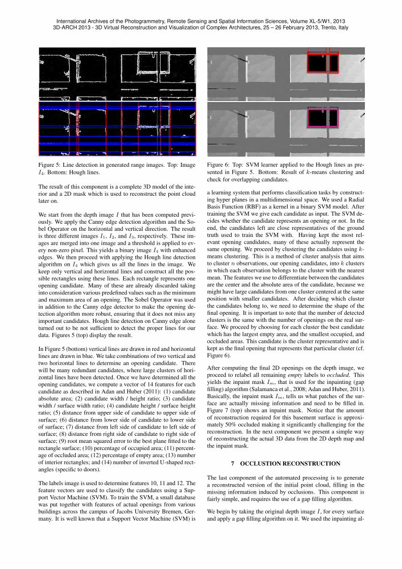
Figure 5: Line detection in generated range images. Top: Image
I4. Bottom: Hough lines.
The result of this component is a complete 3D model of the inte-
rior and a 2D mask which is used to reconstruct the point cloud
later on.
We start from the depth image I that has been computed previ-
ously. We apply the Canny edge detection algorithm and the So-
bel Operator on the horizontal and vertical direction. The result
is three different images I1, I2, and I3, respectively. These im-
ages are merged into one image and a threshold is applied to ev-
ery non-zero pixel. This yields a binary image I4 with enhanced
edges. We then proceed with applying the Hough line detection
algorithm on I4 which gives us all the lines in the image. We
keep only vertical and horizontal lines and construct all the pos-
sible rectangles using these lines. Each rectangle represents one
opening candidate. Many of these are already discarded taking
into consideration various predefined values such as the minimum
and maximum area of an opening. The Sobel Operator was used
in addition to the Canny edge detector to make the opening de-
tection algorithm more robust, ensuring that it does not miss any
important candidates. Hough line detection on Canny edge alone
turned out to be not sufficient to detect the proper lines for our
data. Figures 5 (top) display the result.
In Figure 5 (bottom) vertical lines are drawn in red and horizontal
lines are drawn in blue. We take combinations of two vertical and
two horizontal lines to determine an opening candidate. There
will be many redundant candidates, where large clusters of hori-
zontal lines have been detected. Once we have determined all the
opening candidates, we compute a vector of 14 features for each
candidate as described in Adan and Huber (2011): (1) candidate
absolute area; (2) candidate width / height ratio; (3) candidate
width / surface width ratio; (4) candidate height / surface height
ratio; (5) distance from upper side of candidate to upper side of
surface; (6) distance from lower side of candidate to lower side
of surface; (7) distance from left side of candidate to left side of
surface; (8) distance from right side of candidate to right side of
surface; (9) root mean squared error to the best plane fitted to the
rectangle surface; (10) percentage of occupied area; (11) percent-
age of occluded area; (12) percentage of empty area; (13) number
of interior rectangles; and (14) number of inverted U-shaped rect-
angles (specific to doors).
The labels image is used to determine features 10, 11 and 12. The
feature vectors are used to classify the candidates using a Sup-
port Vector Machine (SVM). To train the SVM, a small database
was put together with features of actual openings from various
buildings across the campus of Jacobs University Bremen, Ger-
many. It is well known that a Support Vector Machine (SVM) is
Figure 6: Top: SVM learner applied to the Hough lines as pre-
sented in Figure 5. Bottom: Result of k-means clustering and
check for overlapping candidates.
a learning system that performs classification tasks by construct-
ing hyper planes in a multidimensional space. We used a Radial
Basis Function (RBF) as a kernel in a binary SVM model. After
training the SVM we give each candidate as input. The SVM de-
cides whether the candidate represents an opening or not. In the
end, the candidates left are close representatives of the ground
truth used to train the SVM with. Having kept the most rel-
evant opening candidates, many of these actually represent the
same opening. We proceed by clustering the candidates using k-means clustering. This is a method of cluster analysis that aims
to cluster n observations, our opening candidates, into k clusters
in which each observation belongs to the cluster with the nearest
mean. The features we use to differentiate between the candidates
are the center and the absolute area of the candidate, because we
might have large candidates from one cluster centered at the same
position with smaller candidates. After deciding which cluster
the candidates belong to, we need to determine the shape of the
final opening. It is important to note that the number of detected
clusters is the same with the number of openings on the real sur-
face. We proceed by choosing for each cluster the best candidate
which has the largest empty area, and the smallest occupied, and
occluded areas. This candidate is the cluster representative and is
kept as the final opening that represents that particular cluster (cf.
Figure 6).
After computing the final 2D openings on the depth image, we
proceed to relabel all remaining empty labels to occluded. This
yields the inpaint mask Im, that is used for the inpainting (gap
filling) algorithm (Salamanca et al., 2008; Adan and Huber, 2011).
Basically, the inpaint mask Im, tells us what patches of the sur-
face are actually missing information and need to be filled in.
Figure 7 (top) shows an inpaint mask. Notice that the amount
of reconstruction required for this basement surface is approxi-
mately 50% occluded making it significantly challenging for the
reconstruction. In the next component we present a simple way
of reconstructing the actual 3D data from the 2D depth map and
the inpaint mask.
7 OCCLUSTION RECONSTRUCTION
The last component of the automated processing is to generate
a reconstructed version of the initial point cloud, filling in the
missing information induced by occlusions. This component is
fairly simple, and requires the use of a gap filling algorithm.
We begin by taking the original depth image I , for every surface
and apply a gap filling algorithm on it. We used the inpainting al-
International Archives of the Photogrammetry, Remote Sensing and Spatial Information Sciences, Volume XL-5/W1, 20133D-ARCH 2013 - 3D Virtual Reconstruction and Visualization of Complex Architectures, 25 – 26 February 2013, Trento, Italy

Figure 8: Views of the reconstructed 3D point cloud. The light red points have been added through the inpaint process.
Figure 7: Top: Inpaint mask. Bottom: Final 2D opening.
Figure 9: Reconstructed depth image.
gorithm provided in OpenCV, namely the Navier-stokes method (Bertalmio
et al., 2001). We use the inpaint mask computed in the previous
component Im. The result of this process is a reconstructed 2D
depth image Ir, having all the missing information filled in. We
then proceed to computing the mean and standard deviation of
the original depth image, in the depth axis, and add Gaussian
noise with the same mean and standard deviation to the newly
reconstructed image, thus yielding the final reconstructed depth
image of the surface If . Adding Gaussian noise to the recon-
structed depth image produces a more natural look and feel of the
inpainted parts.
After computing the reconstructed depth image and adding noise,
we proceed by projecting If back into 3D. This yields the recon-
structed surface point cloud. Figure 9 shows the reconstructed
depth image, from which the 3D point cloud is extrapolated( cf.
Figure 8.
8 EXPERIMENTS AND RESULTS
The interior modeling software is implemented in C/C++ and is
part of the Open Source software 3DTK - The 3D Toolkit. The
input were 3D point clouds acquired by a Riegl VZ-400 terrestrial
laser scanner. The point clouds were reduced to approximately 5
million points per 3D scan by applying an octree based reduction
down to one point per cubic centimeter.
Throughout the text we have visualized the results of all inter-
mediate steps of our pipeline using a data set acquired in the
basement of the Research I building at Jacobs University Bre-
men, Germany. The basement data is very good for testing our
pipeline. Even though it was very fragmented for plane detection,
the pipeline was able to accurately determine the six surfaces of
Figure 10: Seminar room.
International Archives of the Photogrammetry, Remote Sensing and Spatial Information Sciences, Volume XL-5/W1, 20133D-ARCH 2013 - 3D Virtual Reconstruction and Visualization of Complex Architectures, 25 – 26 February 2013, Trento, Italy

the interior. It was ideal for the surface labeling, since it contained
large areas of all three labels, mainly occluded areas, due to nu-
merous pipes running from one side of the room to the other. For
opening detection, the only opening on the surface is occluded by
a vertical pipe, which challenges the SVM in properly choosing
candidates. In the case of windows with thick frames or window
mounted fans, the algorithm is able to avoid detecting multiple
smaller windows, because it checks for overlapping candidates,
in the end keeping the best candidate with the largest empty area,
which is always the whole window.
Furthermore, we want to report the results on a second data set,
which we acquired in a typical seminar room at our university
(cf. Figure 10). It features two windows and the walls are less
occluded.
For the seminar room data the task for the SVM is simplified
since the openings on the surface do not feature any obstructions.
Almost all the opening candidates marked in red overlap very
closely with the real opening. Clustering is again trivial, as there
are clearly two easily distinguishable clusters among the opening
candidates. As before, the best candidate from each cluster is
chosen as a final opening. We again inpaint the range image and
reconstruct the 3D point cloud as shown in Figure 12.
9 CONCLUSIONS AND OUTLOOK
This paper presents a complete and Open Source system for ar-
chitectural 3D interior reconstruction from 3D point clouds. It
consists of fast 3D plane detection, geometry computation by ef-
ficiently calculating intersection of merged planes, semantic la-
beling in terms of occupied, occluded and empty parts, opening
detection using machine learning, and finally 3D point cloud in-
painting to recover occluded parts. The implementation is based
on OpenCV and the 3DTK – The 3D Toolkit and is available on
Sourceforge (Lingemann and Nuchter, 2012).
Identifying and restoring hidden areas behind furniture and clut-
tered objects in indoor scenes is challenging. In this research we
approached this task by dividing it into four components, each
one relying on the outcome of the previous component. The wall
detection and labeling components are highly-reliable, however,
for the opening detection and the reconstruction scene specific
fine tuning was needed. One reason is that the opening detec-
tion vastly depends on the data used to train the Support Vector
Machine. This is one of the drawbacks when using supervised
learning methods. Moreover, we considered windows to be of
rectangular shape. Although, this is a valid assumption, attempt-
ing to detect windows of various shapes would severely increase
the difficulty of the task. For the reconstruction component, de-
spite the fact that we are being provided a reliable inpaint mask
from the previous component, it is difficult to assume what is
actually in the occluded areas. 2D inpainting is one approach
in approximating what the surface would look like. We have to
state, that the best solution to reducing occlusion is to take multi-
ple scans. Thus, future work will incorporate multiple scans and
address the next-best-view planning problem.
So far we have presented a pipeline based on four major compo-
nents. This modularity offers many advantages as each compo-
nent is replaceable by any other approach. In the future, other
components will be added and we will allow for any combination
of these components to be used. One potential improvement for
the opening detection component would be the use of reflectance
images. This would greatly increase the robustness of this com-
ponent. We would be able to generate fewer, more appropriate
opening candidates, instead of generating all the possible ones
from the extracted lines. This can be achieved by exploiting the
intensity information contained in the reflectance image.
Needless to say a lot of work remains to be done. The current
purpose of our software is to simplify and automate the gener-
ation of building models. Our next step will be to extend the
pipeline with an additional component that will put together mul-
tiple scans of interiors and generate the model and reconstructed
point cloud of an entire building. Another way of extending the
pipeline is to add a component that would combine geometrical
analysis of point clouds and semantic rules to detect 3D building
objects. An approach would be to apply a classification of related
knowledge as definition, and to use partial knowledge and am-
biguous knowledge to facilitate the understanding and the design
of a building (Duan et al., 2010).
References
Adan, A. and Huber, D., 2011. 3D reconstruction of interior wall surfacesunder occlusion and clutter. In: Proceedings of 3D Imaging, Modeling,Processing, Visualization and Transmission (3DIMPVT).
Adan, A., Xiong, X., Akinci, B. and Huber, D., 2011. Automatic creationof semantically rich 3D building models from laser scanner data. In:Proceedings of the International Symposium on Automation and Roboticsin Construction (ISARC).
Bertalmio, M., Bertozzi, A. and Sapiro, G., 2001. Navier-stokes, fluiddynamics, and image and video inpainting. In: Proceedings of the IEEEConference on Computer Vision and Pattern Recognition (CVPR 01).,pp. 355–362.
Bohm, J., 2008. Facade detail from incomplete range data. In: Proceed-ings of the ISPRS Congress, Beijing, China.
Bohm, J., Becker, S. and Haala, N., 2007. Model refinement by integratedprocessing of laser scanning and photogrammetry. In: Proceedings of 3DVirtual Reconstruction and Visualization of Complex Architectures (3D-Arch), Zurich, Switzerland.
Borrmann, D., Elseberg, J., Lingemann, K. and Nuchter, A., 2011. The3D Hough Transform for plane detection in point clouds: A review and anew accumulator design. 3D Research.
Bresenham, J. E., 1965. Algorithm for computer control of a digital plot-ter. IBM Systems Journal 4 4(1), pp. 25–30.
Budroni, A. and Bohm, J., 2005. Toward automatic reconstruction of in-teriors from laser data. In: Proceedings of 3D-Arch, Zurich, Switzerland.
Duan, Y., Cruz, C. and Nicolle, C., 2010. Architectural reconstructionof 3D building objects through semantic knowledge management. In:ACIS International Conference on Software Engineering, Artificial Intel-ligence, Networking and Parallel/Distributed Computing.
Elseberg, J., Borrmann, D. and Nuchter, A., 2013. One billion points inthe cloud — an octree for efficient processing of 3d laser scans. JournalPotogrammetry and Remote Sensing.
Fisher, R. B., 2002. Applying knowledge to reverse engeniering prob-lems. In: Proceedings of the International Conference. Geometric Mod-eling and Processing (GMP ’02), Riken, Japan, pp. 149 – 155.
Fruh, C., Jain, S. and Zakhor, A., 2005. Data processing algorithmsfor generating textured 3D building facade meshes from laser scans andcamera images. International Journal of Computer Vision (IJCV) 61(2),pp. 159–184.
Hahnel, D., Burgard, W. and Thrun, S., 2003. Learning compact 3Dmodels of indoor and outdoor environments with a mobile robot. Roboticsand Autonomous Systems 44(1), pp. 15–27.
Hough, P., 1962. Method and means for recognizing complex patterns.US Patent 3069654.
Lingemann, K. and Nuchter, A., 2012. The 3D Toolkit.http://threedtk.de.
International Archives of the Photogrammetry, Remote Sensing and Spatial Information Sciences, Volume XL-5/W1, 20133D-ARCH 2013 - 3D Virtual Reconstruction and Visualization of Complex Architectures, 25 – 26 February 2013, Trento, Italy

Figure 11: Top row: Detected planes in a seminar room. Second row: Detected planes as overlay to the 3D point cloud. Third row:
Image I4 and the Hough lines. Forth row: Opening candidates and the result of the k-means clustering. Fifth row: Inpaint mask and
final 2D openings. Bottom: Reconstructed depth image.
International Archives of the Photogrammetry, Remote Sensing and Spatial Information Sciences, Volume XL-5/W1, 20133D-ARCH 2013 - 3D Virtual Reconstruction and Visualization of Complex Architectures, 25 – 26 February 2013, Trento, Italy

Figure 12: Reconstructed 3D point clouds in the seminar room.
Nuchter, A., Surmann, H., Lingemann, K. and Hertzberg, J., 2003. Se-mantic Scene Analysis of Scanned 3D Indoor Environments. In: Pro-ceedings of the of the 8th International Fall Workshop Vision, Modeling,and Visualization (VMV ’03), Munich, Germany, pp. 215–222.
Pu, S. and Vosselman, G., 2009. Knowledge based reconstruction ofbuilding models from terrestrial laser scanning data. Journal of Pho-togrammetry and Remote Sensing 64(6), pp. 575–584.
Ripperda, N. and Brenner, C., 2009. Application of a formal grammar tofacade reconstruction in semiautomatic and automatic environments. In:Proceedings of AGILE Conference on Geographic Information Science,Hannover, Germany.
Salamanca, S., Merchan, P., Perez, E., Adan, A. and Cerrada, C., 2008.Filling holes in 3D meshes using image restoration algorithms. In: Pro-ceedings of the Symposium on 3D Data Processing, Visualization, andTransmission (3DPVT), Atlanta, Georgia, United States of America.
Stamos, I., Yu, G., Wolberg, G. and Zokai, S., 2006. Application of aformal grammar to facade reconstruction in semiautomatic and automaticenvironments. In: Proceedings of 3D Data Processing, Visualization, andTransmission (3DPVT), pp. 599–606.
Thrun, S., Martin, C., Liu, Y., Hahnel, D., Montemerlo, R. E.,Chakrabarti, D. and Burgard, W., 2004. A real-time expectation max-imization algorithm for acquiring multi-planar maps of indoor environ-ments with mobile robots. IEEETransactions on Robotics 20(3), pp. 433–443.
Willow Garage, 2012. Point cloud library.http://pointclouds.org/.
Xu, L., Oja, E. and Kultanen, P., 1990. A new curve detectionmethod:Randomized Hough Transform (RHT). Pattern Recognition Letters 11,pp. 331–338.
International Archives of the Photogrammetry, Remote Sensing and Spatial Information Sciences, Volume XL-5/W1, 20133D-ARCH 2013 - 3D Virtual Reconstruction and Visualization of Complex Architectures, 25 – 26 February 2013, Trento, Italy


![Locating An IRIS From Image Using Canny And Hough Transform · 2017-11-15 · Hough transform" after the related 1962 patent of Paul Hough.‖[5] In Hough Transform, input image is](https://img.pdfslide.us/doc/110x75/5ebebfab13dd9e6bb364610f/locating-an-iris-from-image-using-canny-and-hough-transform-2017-11-15-hough-transform.jpg)