Interior point algorithm for the optimization of a space ...bonnans/ fileJulien Laurent-Varin Interior point algorithm for the optimization of a space shuttle re-entry trajectory

Julien Laurent-Varin

Interior point algorithm for the optimizationof a space shuttle re-entry trajectory

.

Julien Laurent-Varin, CNES-INRIA-ONERA

Common work with

J. F. Bonnans INRIA, N. Bérend ONERA,

M. Haddou U. Orléans, C. Talbot CNES

[email protected]

http://www-rocq.inria.fr/sydoco/

Introduction

● Context

● Ultimate aims of this work

● Survey

Discretization

Order conditions

Interior Point algorithms

Mesh Refinement

Space Shuttle reentry

Multiarc problems

Julien Laurent-Varin 7th French-Latin American Congress on Applied Mathematics - 2

Introduction


Introduction

● Context


● Survey

Discretization

Order conditions


Mesh Refinement


Multiarc problems


Context

■ A typical mission

Orbiter et Boosteron ground

Booster separation

Retour booster

Rendez-vous with stationOrbital station

End of mission

■ A challenge for optimal control software


Introduction

● Context


● Survey

Discretization

Order conditions


Mesh Refinement


Multiarc problems


Ultimate aims of this work

■ Efficient method for solving optimal controlproblems with path constraints

■ Compute the ascent trajectory of classical launcher■ Compute reentry trajectory of an orbitor■ Compute the whole trajectory of a future space

launcher (with possible rendez-vous)


Introduction

● Context


● Survey

Discretization

Order conditions


Mesh Refinement


Multiarc problems


Survey

[1] J.T. Betts. Survey of numerical methods fortrajectory optimization. AIAA J. of Guidance,Control and Dynamics, 21:193–207, 1998.

[2] J.T. Betts. Practical methods for optimal controlusing nonlinear programming. Society forIndustrial and Applied Mathematics (SIAM),Philadelphia, PA, 2001.


Introduction

Discretization

● Problem descrition (P)

● Discretized Problem (DP)

● Optimal conditions of (DP)

● Optimal conditions of (P)

● Commutative diagram

● Summary

Order conditions


Mesh Refinement


Multiarc problems


Discretization


Introduction

Discretization






● Summary

Order conditions


Mesh Refinement


Multiarc problems


Problem descrition (P)

Consider the optimal control problem (P) :

Min Φ(y(T ));

y(t) = f(u(t), y(t)), t ∈ [0, T ];

y(0) = y0.

(P )

Discretize dynamic with Runge-Kutta method


Introduction

Discretization






● Summary

Order conditions


Mesh Refinement


Multiarc problems


Discretized Problem (DP)

Min Φ(yN );

yk+1 = yk + hk

∑si=1 bif(uki, yki),

yki = yk + hk

∑sj=1 aijf(ukj , ykj),

y0 = y0.

(DP )

[1] W. Hager. Runge-Kutta methods in optimalcontrol and the transformed adjoint system.Numer. Math., 87(2):247–282, 2000.


Introduction

Discretization






● Summary

Order conditions


Mesh Refinement


Multiarc problems


Optimal conditions of (DP)

yk+1 = yk + hk

∑si=1 bif(uki, yki),

yki = yk + hk

∑sj=1 aijf(ukj, ykj),

pk+1 = pk + hk

∑si=1 bify(yki, uki)

T pki,

pki = pk + hk

∑sj=1 aijfy(ykj, ukj)

Tpkj ,

0 = fu(yk, uk)Tpk,

0 = fu(yki, uki)Tpki,

y0 = y0, pN = Φ′(yN ).

(DOC)

Where : b = b and aij =bibj − bjaij

bifor all i, j.

Partitioned RK methods


Introduction

Discretization






● Summary

Order conditions


Mesh Refinement


Multiarc problems


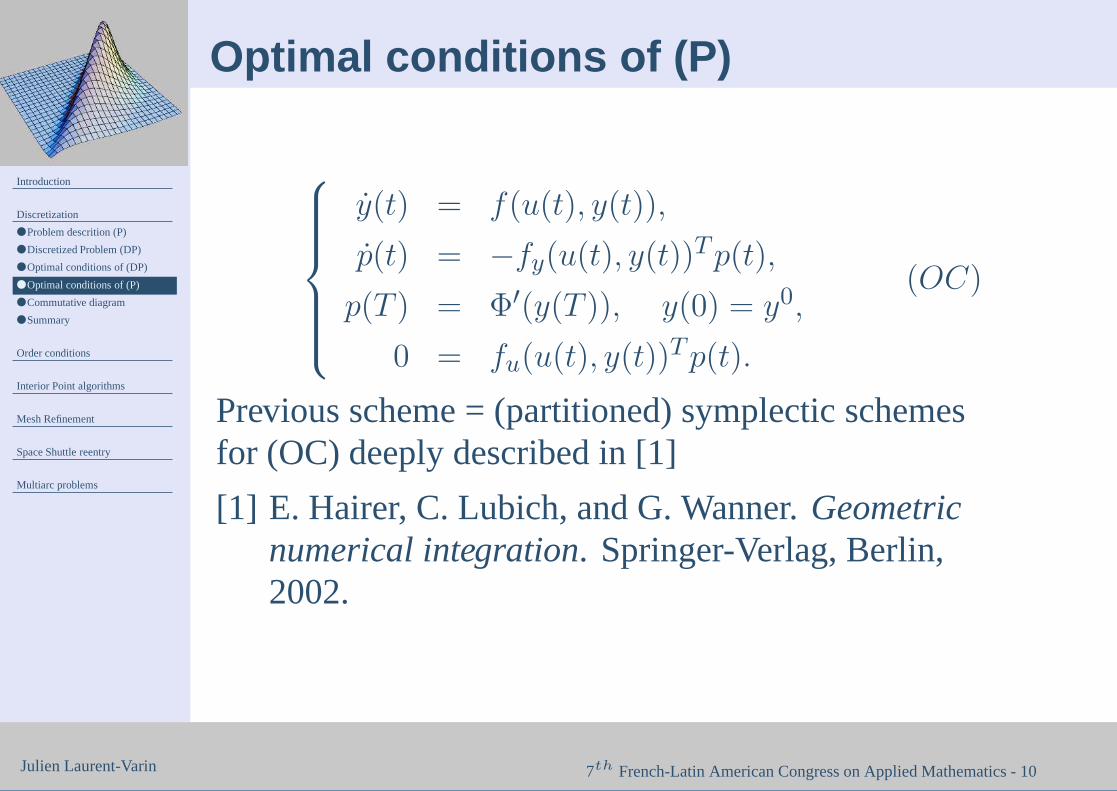
Optimal conditions of (P)

y(t) = f(u(t), y(t)),

p(t) = −fy(u(t), y(t))Tp(t),

p(T ) = Φ′(y(T )), y(0) = y0,

0 = fu(u(t), y(t))Tp(t).

(OC)

Previous scheme = (partitioned) symplectic schemesfor (OC) deeply described in [1]

[1] E. Hairer, C. Lubich, and G. Wanner. Geometricnumerical integration. Springer-Verlag, Berlin,2002.


Introduction

Discretization






● Summary

Order conditions


Mesh Refinement


Multiarc problems


Commutative diagram

(P )discretization−−−−−−−−−−→ (DP )

optimality

conditions

y

optimality

conditions

y

(OC)discretization−−−−−−−−−−→ (DOC)

(D)


Introduction

Discretization






● Summary

Order conditions


Mesh Refinement


Multiarc problems


Summary

Complete error analysis for :■ unconstrained problems■ with strongly convex Hamiltonians

Existing theory for :■ control constraint■ order one state constraints

(Dontchev, Hager)

Open problems :■ Singular arcs■ high order state constraints


Introduction

Discretization

Order conditions

● Order conditions - I

● Order conditions - II

● Order conditions - III

● Symplectic schemes - order 4



Mesh Refinement


Multiarc problems


Order conditions


Introduction

Discretization

Order conditions







Mesh Refinement


Multiarc problems


Order conditions - I

For partitionned Runge-Kutta Schemes, we haveorder conditions based on bi-colored rooted tree. Forexample :

Bi-coloured tree t

i

j

k l

φ(t) = 1/γ(t)s

∑

i,j,k,l=1

biaijajkajl =1

12


Introduction

Discretization

Order conditions







Mesh Refinement


Multiarc problems


Order conditions - II

But our partitionned schemes is particular and havethe following propertise :

bi = bi ∀i = 1, . . . , s

aij = bj −bjbiaji ∀i = 1, . . . , s ∀j = 1, . . . , s

(1)

This propertise leads to computation that can beinterpreted in term of graph computation.


Introduction

Discretization

Order conditions







Mesh Refinement


Multiarc problems


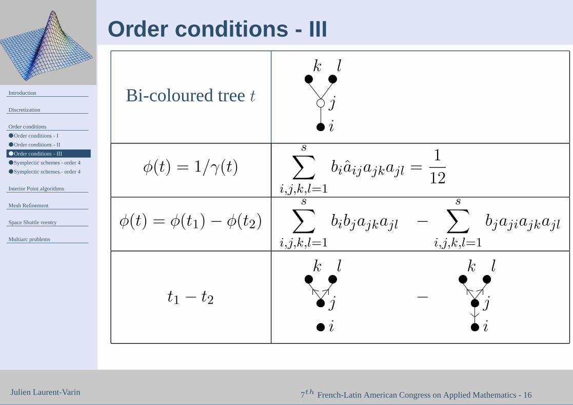
Order conditions - III

Bi-coloured tree t

i

j

k l

φ(t) = 1/γ(t)s

∑

i,j,k,l=1

biaijajkajl =1

12

φ(t) = φ(t1) − φ(t2)

s∑

i,j,k,l=1

bibjajkajl −s

∑

i,j,k,l=1

bjajiajkajl

t1 − t2

i

j

k l

−i

j

k l


Introduction

Discretization

Order conditions







Mesh Refinement


Multiarc problems


Symplectic schemes - order 4

Graph Condition Graph Condition∑ 1

bkalkdkdl =

1

8

∑

ajkdjck =1

24

∑ bibkaikcidk =

5

24

∑

biaijcicj =1

8

∑

c2jdj =1

12

∑

bic3i =

1

4

∑ 1

bkckd

2k =

1

12

∑ 1

b2ld3

l =1

4


Introduction

Discretization

Order conditions







Mesh Refinement


Multiarc problems


Symplectic schemes - order 4

In the previous table, we use the usual notations

dj =∑

i

biaij

andci =

∑

j

aij

.


Introduction

Discretization

Order conditions


● History

● Basic idea

● For our problem

● For our problem

● Combination with mesh

refinement

● Sparsity structure

Mesh Refinement


Multiarc problems




Introduction

Discretization

Order conditions


● History

● Basic idea

● For our problem

● For our problem


refinement


Mesh Refinement


Multiarc problems


History

[1] A.V. Fiacco and G.P. McCormick. Nonlinearprogramming. John Wiley and Sons, Inc., NewYork-London-Sydney, 1968.

[2] L. G. Hacijan. A polynomial algorithm in linearprogramming. Dokl. Akad. Nauk SSSR,244(5):1093–1096, 1979.

[3] N. Karmarkar. A new polynomial-time algorithmfor linear programming. Combinatorica,4(4):373–395, 1984.


Introduction

Discretization

Order conditions


● History

● Basic idea

● For our problem

● For our problem


refinement


Mesh Refinement


Multiarc problems


Basic idea

Transformation of constrained problem (forgetequality constraints in order to simplify presentation)

Min f(x); g(x) ≥ 0 (P )

Logarithmic penalty

Min f(x) − ε ln g(x) (Pε)

Unconstrained problem solved by Newton steps onoptimality conditions, with basic safeguards


Introduction

Discretization

Order conditions


● History

● Basic idea

● For our problem

● For our problem


refinement


Mesh Refinement


Multiarc problems


For our problem

Min

∫ T

0`(u(t), y(t), up, t)dt+ `f (y(T ), up, T );

y(t) = f(u(t), y(t), up, t), t ∈ [0, T ];

yi(0) = y0i ∀i ∈ I0, yi(T ) = yT

i ∀i ∈ IT

a ≤ g(u(t), y(t), up, t) ≤ b, t ∈ [0, T ].

(P )


Introduction

Discretization

Order conditions


● History

● Basic idea

● For our problem

● For our problem


refinement


Mesh Refinement


Multiarc problems


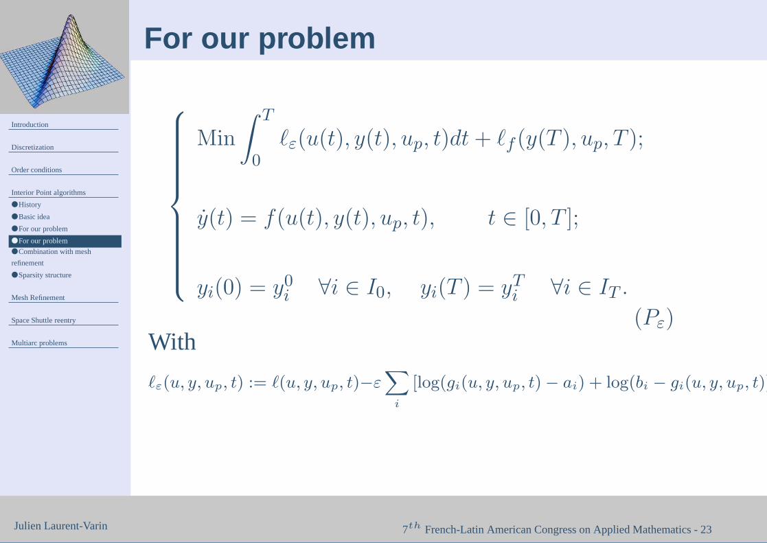
For our problem

Min

∫ T

0`ε(u(t), y(t), up, t)dt+ `f (y(T ), up, T );

y(t) = f(u(t), y(t), up, t), t ∈ [0, T ];

yi(0) = y0i ∀i ∈ I0, yi(T ) = yT

i ∀i ∈ IT .

(Pε)With

`ε(u, y, up, t) := `(u, y, up, t)−εX

i

[log(gi(u, y, up, t) − ai) + log(bi − gi(u, y, up, t))]


Introduction

Discretization

Order conditions


● History

● Basic idea

● For our problem

● For our problem


refinement


Mesh Refinement


Multiarc problems


Combination with mesh refinement

We must have ε ↓ 0 (IP parameter) and E ↓ 0

(Integration error)

Good News : Both can be reduced simultaneously :interpolate values at additional points. Our(somewhat arbitrary) choice :For a fixed ε, we refine mesh until

E ≤ cε; c = 1/10 in our tests.


Introduction

Discretization

Order conditions


● History

● Basic idea

● For our problem

● For our problem


refinement


Mesh Refinement


Multiarc problems


Sparsity structure

A B

C D

■ Band matrix: distributed variables, band QRavailable

■ Full pieces: static parameters■ Solve by elimination of distributed variables


Introduction

Discretization

Order conditions


Mesh Refinement

● Modelisation of error

● Optimal refinement problem

● Maximal gain index

● Resolution of (ORP)


Multiarc problems


Mesh Refinement


Introduction

Discretization

Order conditions


Mesh Refinement






Multiarc problems


Modelisation of error

■ k : index of time step■ ek = Ckh

p+1k : error model (valid for hk small)

estimated by variable order (symplectic) schemes.Adding (qk − 1) points in kth step ⇒ estimate of errorbecomes :

ekqpk


Introduction

Discretization

Order conditions


Mesh Refinement






Multiarc problems


Optimal refinement problem

Reach a specific error estimationMinimise the number of added pointsInteger programming problem with a single nonlinearconstraints

Minq∈NN

N∑

k=1

qk;N

∑

k=1

ekqpk

≤ E (ORP )


Introduction

Discretization

Order conditions


Mesh Refinement






Multiarc problems


Maximal gain index

Definition 1. Maximal marginal gain g and maximal gainindex kg for which the maximum error reduction is obtainedby adding only one point :

g(q) := maxk

ek(

1/qpk − 1/(qk + 1)p)

(2)

kg := argmaxk

ek(

1/qpk − 1/(qk + 1)p)

(3)


Introduction

Discretization

Order conditions


Mesh Refinement






Multiarc problems


Resolution of (ORP)

Algorithm 1. AORP

For k = 1, . . . , N do qk := 1. End for

While∑N

k=1 ek/qpk > E do

Compute kg, the maximal gain index.qkg

:= qkg+ 1.

End While

This algorithm solves (ORP) inO(((E0/E)p + 1)N logN) operations


Introduction

Discretization

Order conditions


Mesh Refinement


● Control variables

● State variables

● Dynamic I

● Dynamic II

● Cost

● Constraints● Result without heating

constraints

● Result (control)

● Discretization

● Result with heating constraints


● Result (state)

● Result (constraint:heating)

● 3D view: no heating constraints

● 3D view: heating constraints

Multiarc problems




Introduction

Discretization

Order conditions


Mesh Refinement



● State variables

● Dynamic I

● Dynamic II

● Cost


constraints


● Discretization



● Result (state)




Multiarc problems


Control variables

µ

γ

α

~V

Bank angle µ Flightpath angle (γ)

Angle of attack (α)


Introduction

Discretization

Order conditions


Mesh Refinement



● State variables

● Dynamic I

● Dynamic II

● Cost


constraints


● Discretization



● Result (state)




Multiarc problems


State variables

z altitude V velocity

λ longitude γ flightpath angle

φ latitude ψ azimuth


Introduction

Discretization

Order conditions


Mesh Refinement



● State variables

● Dynamic I

● Dynamic II

● Cost


constraints


● Discretization



● Result (state)




Multiarc problems


Dynamic I

z = V sin γ

λ =V cos γ sinψ

(z +Re) cosφ

φ =V cos γ cosψ

z +Re


Introduction

Discretization

Order conditions


Mesh Refinement



● State variables

● Dynamic I

● Dynamic II

● Cost


constraints


● Discretization



● Result (state)




Multiarc problems


Dynamic II

V = −Dm

− g sin γ

γ =L cosµ

mV+

(

V 2

z +Re− g

)

cos γ

V

ψ =L sinµ

mV cos γ+

V

z +Recos γ sinψ tanφ


Introduction

Discretization

Order conditions


Mesh Refinement



● State variables

● Dynamic I

● Dynamic II

● Cost


constraints


● Discretization



● Result (state)




Multiarc problems


Cost

Max crossrange (final latitude)

J := φ(T )


Introduction

Discretization

Order conditions


Mesh Refinement



● State variables

● Dynamic I

● Dynamic II

● Cost


constraints


● Discretization



● Result (state)




Multiarc problems


Constraints

Control constraints :{

0◦ ≤ α ≤ 50◦

−90◦ ≤ µ ≤ 0◦

Mixed control-state contraint (Heating flux) :

q(α)√ρV 3.07 ≤ Qmax

withq(α) = c0 + c1α+ c2α

2 + c3α3


Introduction

Discretization

Order conditions


Mesh Refinement



● State variables

● Dynamic I

● Dynamic II

● Cost


constraints


● Discretization



● Result (state)




Multiarc problems


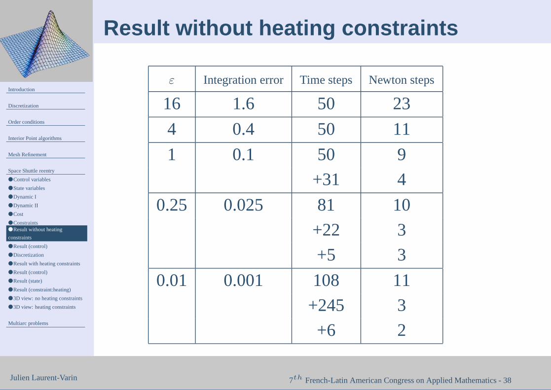
Result without heating constraints

ε Integration error Time steps Newton steps

16 1.6 50 23

4 0.4 50 11

1 0.1 50 9

+31 4

0.25 0.025 81 10

+22 3

+5 3

0.01 0.001 108 11

+245 3

+6 2


Introduction

Discretization

Order conditions


Mesh Refinement



● State variables

● Dynamic I

● Dynamic II

● Cost


constraints


● Discretization



● Result (state)




Multiarc problems


Result (control)

0 400 800 1200 1600 2000 240016

18

20

22

24

26

28Angle of attack (deg)

0 400 800 1200 1600 2000 2400-80

-70

-60

-50

-40

-30

-20

-10

0Bank angle (deg)


Introduction

Discretization

Order conditions


Mesh Refinement



● State variables

● Dynamic I

● Dynamic II

● Cost


constraints


● Discretization



● Result (state)




Multiarc problems


Discretization

0 200 400 600 800 1000 1200 1400 1600 1800 20000.0000

0.0001

0.0002

0.0003

0.0004

0.0005

0.0006

0.0007

0.0008

0.0009


Introduction

Discretization

Order conditions


Mesh Refinement



● State variables

● Dynamic I

● Dynamic II

● Cost


constraints


● Discretization



● Result (state)




Multiarc problems


Result with heating constraints

We add the constraint of heating and we compare theresults


Introduction

Discretization

Order conditions


Mesh Refinement



● State variables

● Dynamic I

● Dynamic II

● Cost


constraints


● Discretization



● Result (state)




Multiarc problems


Result (control)

0 400 800 1200 1600 2000 240016

18

20

22

24

26

28

30Angle of attack (deg)

0 400 800 1200 1600 2000 2400-80

-70

-60

-50

-40

-30

-20

-10

0Bank angle (deg)


Introduction

Discretization

Order conditions


Mesh Refinement



● State variables

● Dynamic I

● Dynamic II

● Cost


constraints


● Discretization



● Result (state)




Multiarc problems


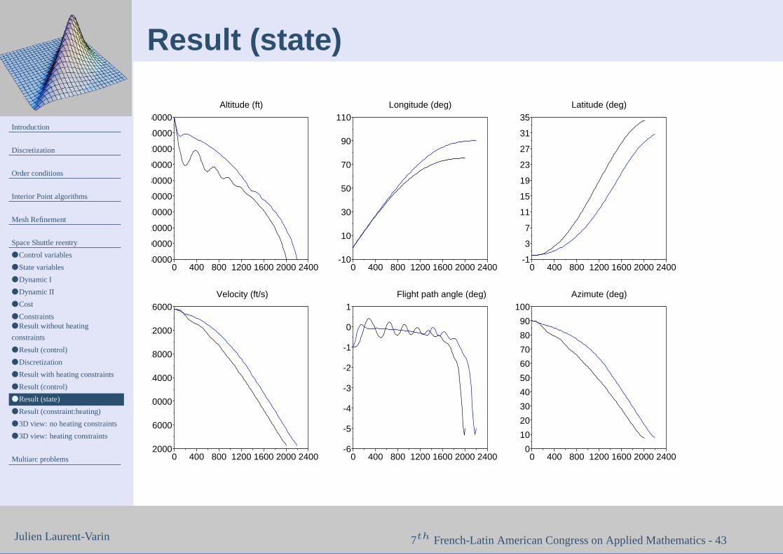
Result (state)

0 400 800 1200 1600 2000 240080000

100000

120000

140000

160000

180000

200000

220000

240000

260000Altitude (ft)

0 400 800 1200 1600 2000 2400-10

10

30

50

70

90

110Longitude (deg)

0 400 800 1200 1600 2000 2400-1

3

7

11

15

19

23

27

31

35Latitude (deg)

0 400 800 1200 1600 2000 24002000

6000

10000

14000

18000

22000

26000Velocity (ft/s)

0 400 800 1200 1600 2000 2400-6

-5

-4

-3

-2

-1

0

1Flight path angle (deg)

0 400 800 1200 1600 2000 24000

10

20

30

40

50

60

70

80

90

100Azimute (deg)


Introduction

Discretization

Order conditions


Mesh Refinement



● State variables

● Dynamic I

● Dynamic II

● Cost


constraints


● Discretization



● Result (state)




Multiarc problems


Result (constraint:heating)

0 400 800 1200 1600 2000 24000

20

40

60

80

100

120

140

160

180

Heating


Introduction

Discretization

Order conditions


Mesh Refinement



● State variables

● Dynamic I

● Dynamic II

● Cost


constraints


● Discretization



● Result (state)




Multiarc problems


3D view: no heating constraints

8

11

14

17

20

23

26

h/10^4

-10

0

10

20

30

40

50

60

70

80

phi-1 3 7 11 15 19 23 27 31 35theta


Introduction

Discretization

Order conditions


Mesh Refinement



● State variables

● Dynamic I

● Dynamic II

● Cost


constraints


● Discretization



● Result (state)




Multiarc problems


3D view: heating constraints

8

11

14

17

20

23

26

h/10^4

0

10

20

30

40

50

60

70

80

90

100

phi-1 3 7 11 15 19 23 27 31theta


Introduction

Discretization

Order conditions


Mesh Refinement


Multiarc problems

● Scenario graph

● Edges: variables

● A view after discretization

● Edges: cost and constraints

● Vertices: variables

● Vertices: cost and constraints

● Cost of factorization and solve

● Perspectives

● Some references


Multiarc problems


Introduction

Discretization

Order conditions


Mesh Refinement


Multiarc problems

● Scenario graph







● Perspectives

● Some references


Scenario graph

1

42

5

3

6

■ V set of vertices■ E set of edges■ Edges: Distributed in time cost and constraints■ Vertices: Junction conditions, cost and constraints


Introduction

Discretization

Order conditions


Mesh Refinement


Multiarc problems

● Scenario graph







● Perspectives

● Some references


Edges: variables

■ Edge E 3 e = (i, j)

■ y(t) ∈ IRne: state■ u(t) ∈ IRme: control■ π ∈ IRre: “static” optimization parameters


Introduction

Discretization

Order conditions


Mesh Refinement


Multiarc problems

● Scenario graph







● Perspectives

● Some references


A view after discretization


Introduction

Discretization

Order conditions


Mesh Refinement


Multiarc problems

● Scenario graph







● Perspectives

● Some references


Edges: cost and constraints

■ `e(t, y(t), u(t), π): Distributed cost■ y(t) = fe(t, y(t), u(t), π): Dynamics■ ge(t, y(t), u(t), π) ≤ 0: Distributed

constraints

■ The value function over arc = integral of costfunction.

■ Feasibility = dynamics are satisfied and distributedconstraints hold.


Introduction

Discretization

Order conditions


Mesh Refinement


Multiarc problems

● Scenario graph







● Perspectives

● Some references


Vertices: variables

■ Vertice j ∈ V

■ Variables zj ∈ IRnj

■ Includes copy of boundary (initial of final) state yBeand parameters πe of connected edges

■ Possibility of other variables


Introduction

Discretization

Order conditions


Mesh Refinement


Multiarc problems

● Scenario graph







● Perspectives

● Some references


Vertices: cost and constraints

■ `i(z): Cost■ yB

e = ze: Copy constraints■ gi(z)) = 0: Equality constraints■ gi(z)) ≤ 0: Inequality constraints


Introduction

Discretization

Order conditions


Mesh Refinement


Multiarc problems

● Scenario graph







● Perspectives

● Some references


Cost of factorization and solve

■ Arcs: O(n2NT )

- n number of state variables- NT average number of time steps per arc

■ Vertices (junctions): O(n) size linear systems- Recursive elimination, starting from leaves- O(n3) operations for each (elimination of) vertex

■ Total number of operations:

n2O(|E|NT + n|V |)

Seems to be the least possible number !


Introduction

Discretization

Order conditions


Mesh Refinement


Multiarc problems

● Scenario graph







● Perspectives

● Some references


Perspectives

■ Implementation of multi-arc methodology■ Test on various examples■ Analysis of convergence (difficult)

- Vanishing parameter ε- Mesh refinement


Introduction

Discretization

Order conditions


Mesh Refinement


Multiarc problems

● Scenario graph







● Perspectives

● Some references


Some references

[1] J. Laurent-Varin, N. Bérend, F. Bonnans,M. Haddou, and C. Talbot. On the refinement ofdiscretization for optimal control problems. 16th

IFAC SYMPOSIUM Automatic Control inAerospace, 14-18 june, St. Petersburg, Russia.

[2] J Laurent-Varin and F Bonnans. Computation oforder conditions for symplectic partitionedRunge-Kutta schemes with application to optimalcontrol. Technical Report RR 5398, INRIA,2004.


56-1

Documents

Interior point algorithm for the optimization of a space ...bonnans/ fileJulien Laurent-Varin Interior point algorithm for the optimization of a space shuttle re-entry trajectory