A SPECIALIZED INTERIOR-POINT ALGORITHM FOR MULTICOMMODITY

A SPECIALIZED INTERIOR-POINT ALGORITHM FORMULTICOMMODITY NETWORK FLOWS∗

JORDI CASTRO†

SIAM J. OPTIM. c© 2000 Society for Industrial and Applied MathematicsVol. 10, No. 3, pp. 852–877

Abstract. Despite the efficiency shown by interior-point methods in large-scale linear pro-gramming, they usually perform poorly when applied to multicommodity flow problems. The newspecialized interior-point algorithm presented here overcomes this drawback. This specialization usesboth a preconditioned conjugate gradient solver and a sparse Cholesky factorization to solve a linearsystem of equations at each iteration of the algorithm. The ad hoc preconditioner developed byexploiting the structure of the problem is instrumental in ensuring the efficiency of the method. Animplementation of the algorithm is compared to state-of-the-art packages for multicommodity flows.The computational experiments were carried out using an extensive set of test problems, with sizes ofup to 700,000 variables and 150,000 constraints. The results show the effectiveness of the algorithm.

Key words. interior-point methods, linear programming, multicommodity flows, network pro-gramming

AMS subject classifications. 90C05, 90C06, 90C35

PII. S1052623498341879

1. Introduction. Multicommodity problems usually have many variables andconstraints, which makes it difficult for them to be solved by general procedures. Thishas led to the formulation of specialized methods. However, some of the largest andmost difficult multicommodity problems are still challenging even for these special-izations. The algorithm presented in this paper has three main features. First, it hasproven to be computationally efficient and robust in the solution of a wide range ofproblems, not just for some specific kind of multicommodity instances. Second, itis a specialized primal-dual interior-point algorithm, so it globally converges to theoptimum in polynomial time, unlike other methods that provide an ε-approximatesolution (e.g., [17]). And finally, it has been able to efficiently solve large instancesof Patient Distribution System (PDS) problems [7]. This class of problems is com-monly used as a de facto standard for testing the performance of multicommoditycodes. With our algorithm we solved the PDS90 and PDS100 instances in a relativelyreasonable amount of time. (In [17] an approximate solution is provided at most forPDS80.)

Most of the specialized methods attempt to exploit in some way the block struc-ture of the multicommodity problem. Among the earlier approaches, we find primalpartitioning and the price and resource directive decompositions (see [2, Chap. 17]and [21] for details). Of these three methods, the first two were regarded as the mostsuccessful in [3]. Despite this, no implementation of primal partitioning has been ableto solve large problems significantly faster than the state-of-the-art simplex codes.For instance, the recent primal partitioning package PPRN [6] was, on average, nomore than an order of magnitude faster than the primal simplex code of MINOS 5.3.In some cases, accurate implementations of the dual simplex—preceded by a warm

∗Received by the editors July 13, 1998; accepted for publication (in revised form) October 6,1999; published electronically May 2, 2000. This work was partially supported by Iberdrola S.A.grant 95-005 and by CICYT project TAP96-1044-J02-93.

http://www.siam.org/journals/siopt/10-3/34187.html†Statistics and Operations Research Department, Universitat Politecnica de Catalunya, Campus

Sud, Pau Gargallo 5, 08028 Barcelona, Spain ([email protected]).

852

INTERIOR-POINT ALGORITHM FOR MULTICOMMODITY FLOWS 853

start based on solving minimum-cost network problems for each commodity—caneven outperform primal partitioning multicommodity specializations (see [13] for acomparison of PPRN and the network+dual solver of CPLEX 3.0). In this paper, weshow that our algorithm, in general, outperforms both PPRN and CPLEX 4.0 and,in some cases, by more than an order of magnitude.

The other method regarded as successful in [3], the price directive or Dantzig–Wolfe decomposition, belongs to the class of cost decomposition approaches for multi-commodity flows (see [13], [15], and [33] for recent variants based on bundle methods,analytic centers, and smooth penalty functions, respectively). A recent computationalstudy [13] showed that these are promising approaches for solving a wide variety ofproblems. However, for some classes of instances—typically difficult problems withlarge networks and not many commodities such as the PDS ones—our interior-pointapproach seems to give considerably better performance. Furthermore, Frangioni [12]noted that the particular cost decomposition method of [13] might sometimes requirethe algorithmic parameters to be tuned if performances are to be the best possible,whereas our algorithm works well with default values.

Interior-point methods have also been applied in the past. For the single-commodity case, efficient specializations were developed by Resende and others [26,28, 29, 30]. These specializations relied on the use of preconditioned conjugate gradi-ent (PCG) solvers. The preconditioners developed, though efficient, were appropriateonly for single-commodity problems. The first reported attempt at solving multi-commodity problems by an interior-point method was probably that described in [1].However, the general implementation of Karmarkar’s projective algorithm used therewas outperformed by a simplex specialized algorithm in the solution of small-size mul-ticommodity instances. Alternative and more efficient approaches were developed inthe following years. In fact, the best complexity bound known for multicommodityproblems is provided by the two interior-point algorithms described in [19] and [20],though none of these papers provided computational results. In [18], Kamath et al.applied a variant of Karmarkar’s projective algorithm using a PCG solver. However,their preconditioner did not take advantage of the multicommodity structure. Anattempt to exploit this structure was made in [9] by Choi and Goldfarb. Thoughthe decomposition scheme they presented is similar to the one in this paper, thesolution procedure differs substantially. Choi and Goldfarb suggest solving a fairlydense matrix positive definite linear system that appears during the decompositionstage by means of parallel and vector processing, whereas we apply a PCG method,which enables large problems to be solved efficiently using a midsize workstation. Adifferent interior-point approach was developed in [31], using a barrier function todecompose the problem. This strategy provided approximate solutions for some ofthe large PDS problems (up to PDS70). However, as will be shown, our methodgives more accurate solutions. Finally, Portugal et al. introduced in [27] a specializedinterior-point algorithm based solely on a PCG, unlike our method, which combinesPCG with direct factorizations. The proposed preconditioner was an extension of thatdeveloped in [26] by the same authors for single-commodity flows. No computationalresults were reported in [27] for the solution of multicommodity problems using thispreconditioner.

This paper is organized as follows. Section 2 presents the formulation of theproblem to be solved. Section 3 outlines the primal-dual algorithm, and in section 4we develop the specialization for multicommodity problems. Section 5 describes someimplementation details of this specialization. Finally, section 6 gives computationalresults that show the efficiency of the algorithm.

854 JORDI CASTRO

2. Problem formulation. Let G = (N ,A) be a directed graph, where N is aset of m + 1 nodes and A is a set of n arcs, and let K be a set of k commoditiesto be routed through the network represented by G. We shall also consider that thearcs of the network have a capacity for all the commodities, which will be known asthe mutual capacity. So, the multicommodity network flow (MCNF) problem can beformulated as follows:

minx(1),...,x(k)

k∑

i=1

c(i)T

x(i)(1)

subject to ANx(i) = b(i), i = 1, . . . , k,(2)k∑

i=1

x(i) ≤ bmc,(3)

0 ≤ x(i) ≤ x(i), i = 1, . . . , k.(4)

Vectors x(i) ∈ Rn and c(i) ∈ Rn are the flow and cost arrays for each commodity i,i = 1, . . . , k. AN ∈ Rm×n is the node-arc incidence matrix, where each column isrelated to an arc a ∈ A, and has only nonzero coefficients in those rows associatedwith the origin and destination nodes of a (with coefficients 1 and −1, respectively).We shall assume that AN is a full row-rank matrix. This can always be guaranteedby removing any of the (redundant) node balance constraints. b(i) ∈ Rm is the vectorof supplies and demands for commodity i at the nodes of the network. Equation(3) represents the mutual capacity constraints, where bmc ∈ Rn. Constraints (4) aresimple bounds on the flows, x(i) ∈ Rn, i = 1, . . . , k, being the upper bounds. Theseupper bounds represent individual capacities of the arcs for each commodity.

Introducing the slacks smc for the mutual capacity constraints, (3) can be rewrit-ten as

k∑

i=1

x(i) + smc = bmc.(5)

We can consider that the slacks smc are upper bounded by bmc, since all the vectorsx(i) in (5) have nonzero components. This gives

0 ≤ smc ≤ bmc.(6)

The MCNF problem can then be recast as

min (1) subject to (2), (4), (5), and (6).(7)

3. Outline of the primal-dual interior-point algorithm. Let us considerthe linear programming problem

min cT x

subject to Ax = b,

x ≥ x ≥ 0,

(8)

where x ∈ Rn, x ∈ Rn are the upper bounds, c ∈ Rn, b ∈ Rm, and A ∈ Rm×n is a fullrow-rank matrix. The dual of (8) is

max bT y − xT w

subject to AT y + z − w = c,

z ≥ 0, w ≥ 0,

(9)


where y ∈ Rm are the dual variables and z ∈ Rn and w ∈ Rn are the dual slacks.Note that the MCNF problem, as defined in (7), fits the formulation of (8), wheren = (k + 1)n and m = km + n.

Replacing the inequalities in (8) by a logarithmic barrier in the objective function,with parameter µ, and considering the slacks f = x− x, it can be seen that the KKTfirst order optimality conditions of (8) and (9) are equivalent to the following systemof nonlinear equations (see [32] for a comprehensive description):

bxz ≡ µen −XZen = 0,

bfw ≡ µen − FWen = 0,

bb ≡ b−Ax = 0,(10)

bc ≡ c− (AT y + z − w) = 0,

(x, z, w) ≥ 0, x ≥ x,

where en is the n-dimensional vector of 1’s; X, Z, F , and W are diagonal matricesdefined as M ∈ Rn×n = diag(m1, . . . , mn); and the vectors b∗ define the left-hand-sideterms of (10). Note that we did not include the slacks equation x + f = x in (10).Instead we replaced the slacks f by x − x, reducing by n the number of equationsand variables. This forces the primal variables x of the iterates obtained during thesolution of (10) to always be interior in relation to their upper bounds.

The solutions of system (10)—considering inequalities as strict inequalities—fordifferent µ values gives rise to an arc of strictly feasible points known as the centralpath. As µ tends to 0, the solutions of (10) converge to those of the original primaland dual problems. A path-following algorithm attempts to follow the central path,computing (10)—in long-step methods—through a damped Newton’s method togetherwith the reduction of the barrier parameter µ at each iteration of the algorithm. Thepath-following algorithm considered for the specialization uses the reduction formulaµ = 0.1(xT z+fT w)/2n. It can be seen [32] that obtaining Newton’s direction amountsto finding dy and then computing dx, dw, dz, in

(AΘAT )dy = bb + AΘr,

dx = Θ(AT dy − r),(11)

dw = F−1(bfw + Wdx),

dz = bc + dw −AT dy,

where

r = F−1bfw + bc −X−1bxz, r ∈ Rn,(12)

Θ = FX(ZF + XW )−1, Θ ∈ Rn×n.(13)

Note that Θ is a positive definite diagonal matrix, since it is nothing but a productof positive definite diagonal matrices. Since A is a full row-rank matrix, AΘAT isalso positive definite. It is quite clear that the main computational burden of thealgorithm is the repeated solution of the linear system

(AΘAT )dy = b,(14)

where b denotes bb + AΘr in (11). The performance of any primal-dual multicom-modity specialization relies on the efficient solution of (14).

856 JORDI CASTRO

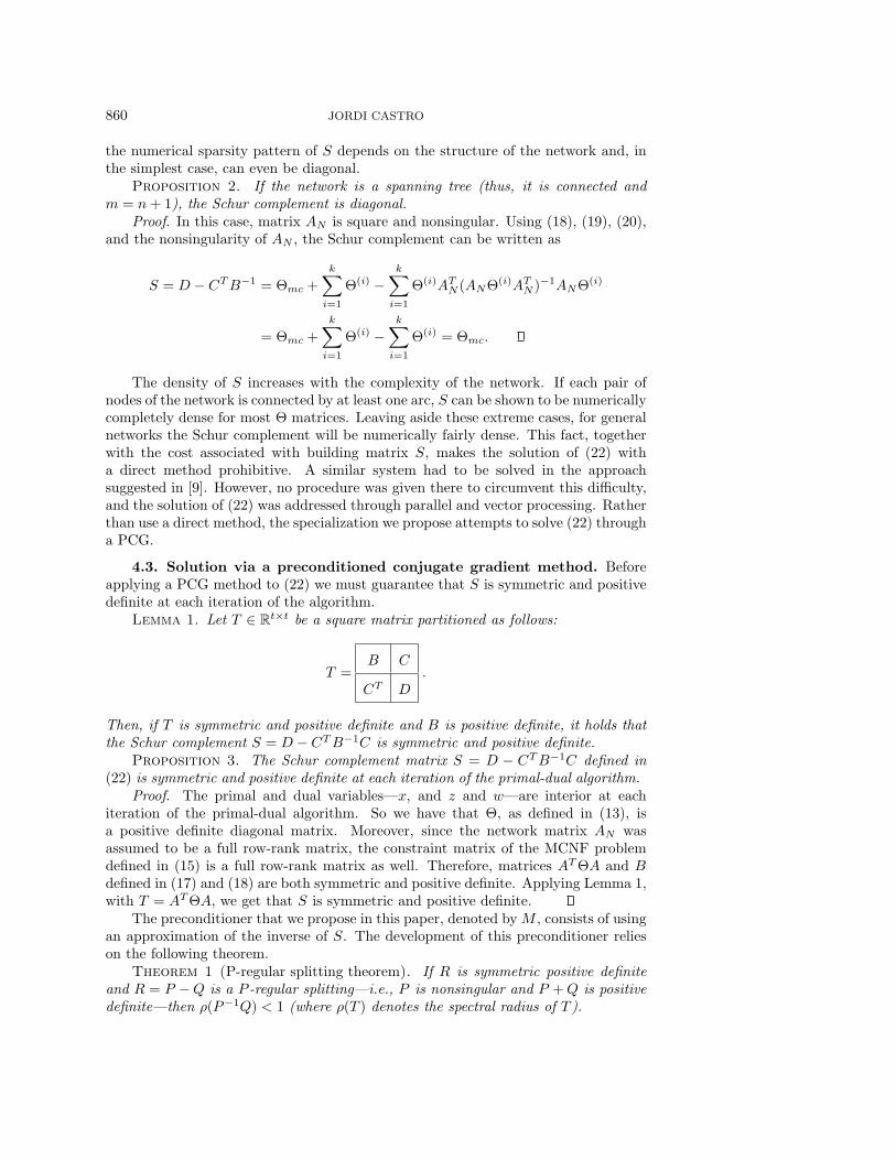
(a) (b)

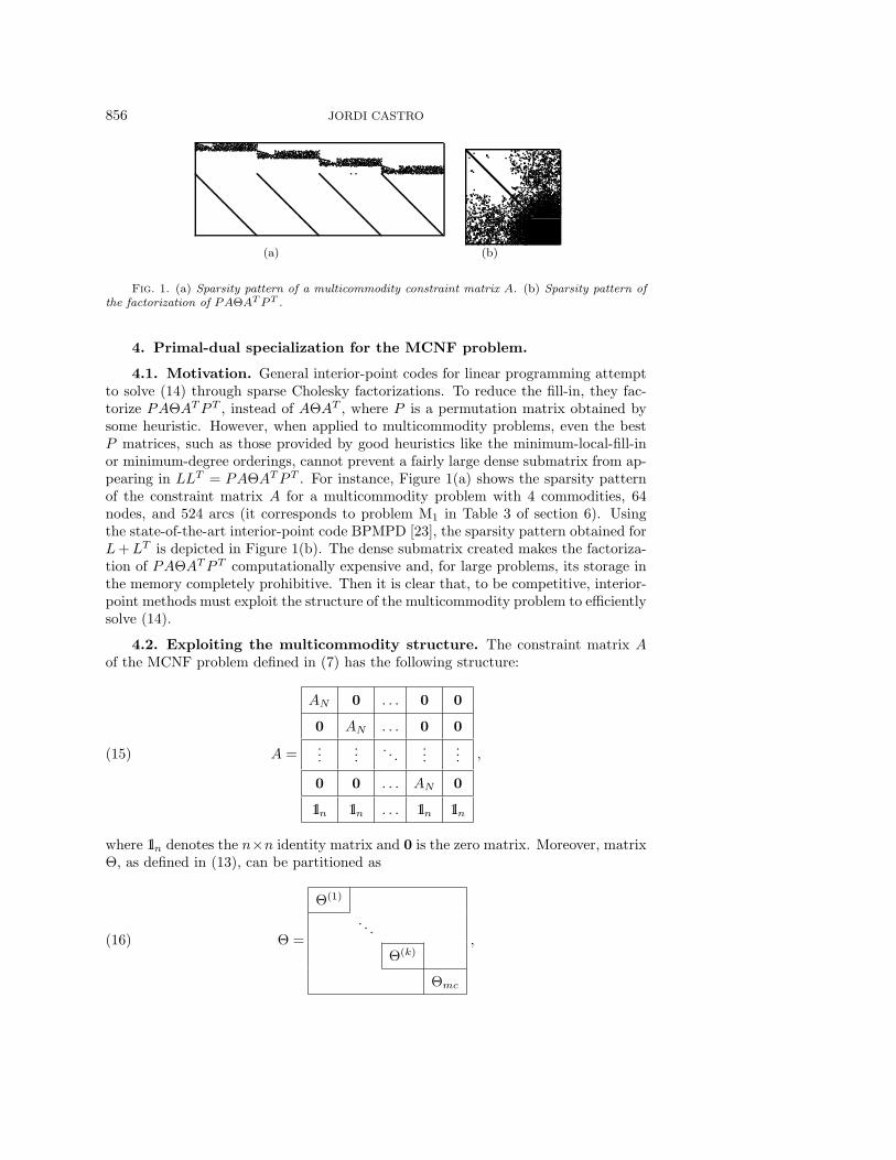
Fig. 1. (a) Sparsity pattern of a multicommodity constraint matrix A. (b) Sparsity pattern ofthe factorization of PAΘAT P T .

4. Primal-dual specialization for the MCNF problem.

4.1. Motivation. General interior-point codes for linear programming attemptto solve (14) through sparse Cholesky factorizations. To reduce the fill-in, they fac-torize PAΘAT PT , instead of AΘAT , where P is a permutation matrix obtained bysome heuristic. However, when applied to multicommodity problems, even the bestP matrices, such as those provided by good heuristics like the minimum-local-fill-inor minimum-degree orderings, cannot prevent a fairly large dense submatrix from ap-pearing in LLT = PAΘAT PT . For instance, Figure 1(a) shows the sparsity patternof the constraint matrix A for a multicommodity problem with 4 commodities, 64nodes, and 524 arcs (it corresponds to problem M1 in Table 3 of section 6). Usingthe state-of-the-art interior-point code BPMPD [23], the sparsity pattern obtained forL + LT is depicted in Figure 1(b). The dense submatrix created makes the factoriza-tion of PAΘAT PT computationally expensive and, for large problems, its storage inthe memory completely prohibitive. Then it is clear that, to be competitive, interior-point methods must exploit the structure of the multicommodity problem to efficientlysolve (14).

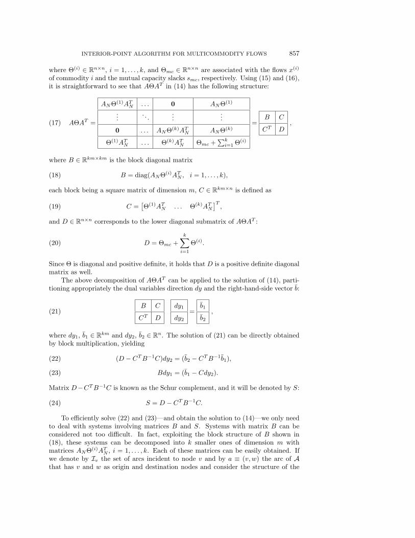
4.2. Exploiting the multicommodity structure. The constraint matrix Aof the MCNF problem defined in (7) has the following structure:

A =

AN 0 . . . 0 0

0 AN . . . 0 0...

.... . .

......

0 0 . . . AN 0

1ln 1ln . . . 1ln 1ln

,(15)

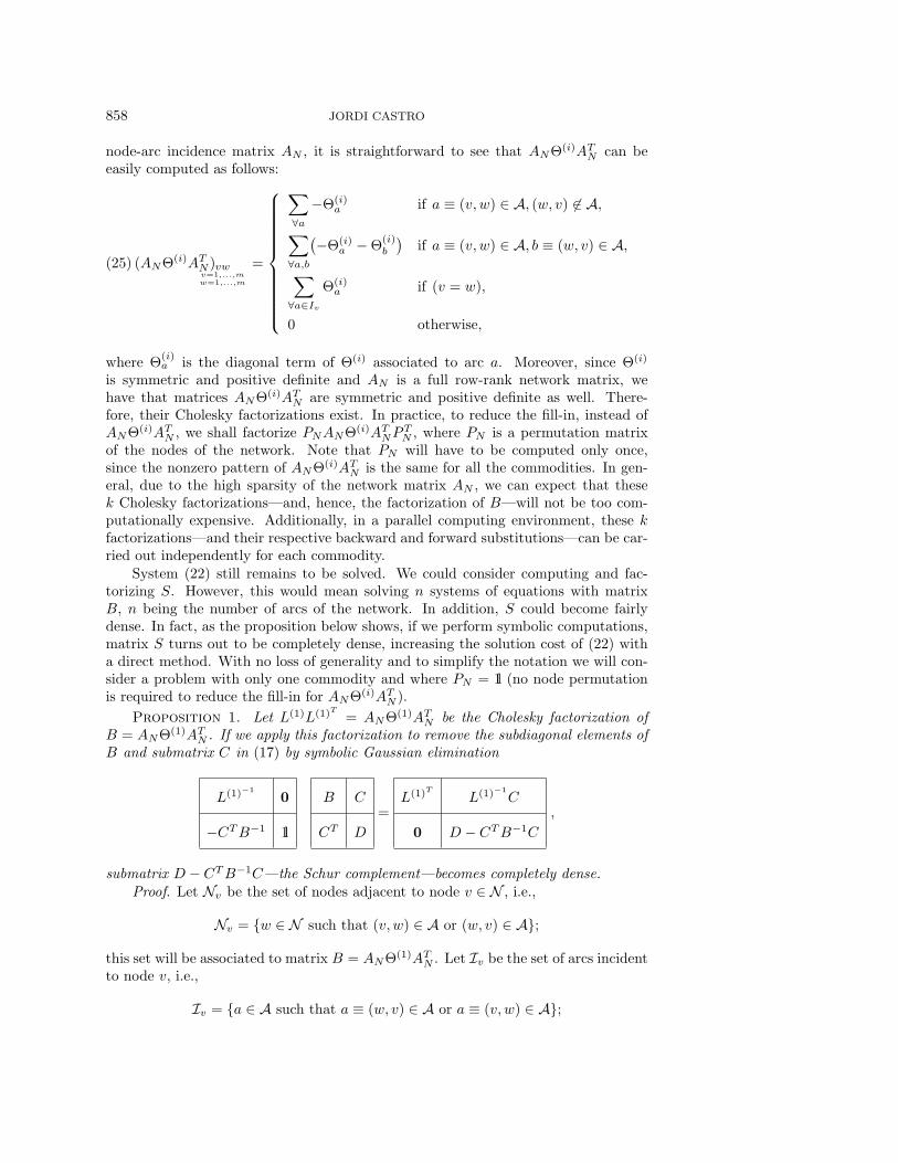
where 1ln denotes the n×n identity matrix and 0 is the zero matrix. Moreover, matrixΘ, as defined in (13), can be partitioned as

Θ =

Θ(1)

. . .

Θ(k)

Θmc

,(16)


where Θ(i) ∈ Rn×n, i = 1, . . . , k, and Θmc ∈ Rn×n are associated with the flows x(i)

of commodity i and the mutual capacity slacks smc, respectively. Using (15) and (16),it is straightforward to see that AΘAT in (14) has the following structure:

AΘAT =

ANΘ(1)ATN . . . 0 ANΘ(1)

.... . .

......

0 . . . ANΘ(k)ATN ANΘ(k)

Θ(1)ATN . . . Θ(k)AT

N Θmc +∑k

i=1 Θ(i)

=B C

CT D,(17)

where B ∈ Rkm×km is the block diagonal matrix

B = diag(ANΘ(i)ATN , i = 1, . . . , k),(18)

each block being a square matrix of dimension m, C ∈ Rkm×n is defined as

C =[Θ(1)AT

N . . . Θ(k)ATN

]T,(19)

and D ∈ Rn×n corresponds to the lower diagonal submatrix of AΘAT :

D = Θmc +k∑

i=1

Θ(i).(20)

Since Θ is diagonal and positive definite, it holds that D is a positive definite diagonalmatrix as well.

The above decomposition of AΘAT can be applied to the solution of (14), parti-tioning appropriately the dual variables direction dy and the right-hand-side vector b:

B C

CT D

dy1

dy2

=b1

b2

,(21)

where dy1, b1 ∈ Rkm and dy2, b2 ∈ Rn. The solution of (21) can be directly obtainedby block multiplication, yielding

(D − CT B−1C)dy2 = (b2 − CT B−1b1),(22)

Bdy1 = (b1 − Cdy2).(23)

Matrix D−CT B−1C is known as the Schur complement, and it will be denoted by S:

S = D − CT B−1C.(24)

To efficiently solve (22) and (23)—and obtain the solution to (14)—we only needto deal with systems involving matrices B and S. Systems with matrix B can beconsidered not too difficult. In fact, exploiting the block structure of B shown in(18), these systems can be decomposed into k smaller ones of dimension m withmatrices ANΘ(i)AT

N , i = 1, . . . , k. Each of these matrices can be easily obtained. Ifwe denote by Iv the set of arcs incident to node v and by a ≡ (v, w) the arc of Athat has v and w as origin and destination nodes and consider the structure of the

858 JORDI CASTRO

node-arc incidence matrix AN , it is straightforward to see that ANΘ(i)ATN can be

easily computed as follows:

(ANΘ(i)ATN )vwv=1,...,mw=1,...,m

=

∑

∀a

−Θ(i)a if a ≡ (v, w) ∈ A, (w, v) 6∈ A,

∑

∀a,b

(−Θ(i)a −Θ(i)

b

)if a ≡ (v, w) ∈ A, b ≡ (w, v) ∈ A,

∑

∀a∈Iv

Θ(i)a if (v = w),

0 otherwise,

(25)

where Θ(i)a is the diagonal term of Θ(i) associated to arc a. Moreover, since Θ(i)

is symmetric and positive definite and AN is a full row-rank network matrix, wehave that matrices ANΘ(i)AT

N are symmetric and positive definite as well. There-fore, their Cholesky factorizations exist. In practice, to reduce the fill-in, instead ofANΘ(i)AT

N , we shall factorize PNANΘ(i)ATNPT

N , where PN is a permutation matrixof the nodes of the network. Note that PN will have to be computed only once,since the nonzero pattern of ANΘ(i)AT

N is the same for all the commodities. In gen-eral, due to the high sparsity of the network matrix AN , we can expect that thesek Cholesky factorizations—and, hence, the factorization of B—will not be too com-putationally expensive. Additionally, in a parallel computing environment, these kfactorizations—and their respective backward and forward substitutions—can be car-ried out independently for each commodity.

System (22) still remains to be solved. We could consider computing and fac-torizing S. However, this would mean solving n systems of equations with matrixB, n being the number of arcs of the network. In addition, S could become fairlydense. In fact, as the proposition below shows, if we perform symbolic computations,matrix S turns out to be completely dense, increasing the solution cost of (22) witha direct method. With no loss of generality and to simplify the notation we will con-sider a problem with only one commodity and where PN = 1l (no node permutationis required to reduce the fill-in for ANΘ(i)AT

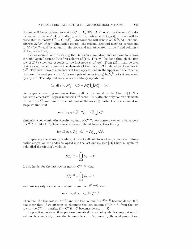
N ).Proposition 1. Let L(1)L(1)T

= ANΘ(1)ATN be the Cholesky factorization of

B = ANΘ(1)ATN . If we apply this factorization to remove the subdiagonal elements of

B and submatrix C in (17) by symbolic Gaussian elimination

L(1)−10

−CT B−1 1l

B C

CT D

=L(1)T

L(1)−1C

0 D − CT B−1C

,

submatrix D − CT B−1C—the Schur complement—becomes completely dense.Proof. Let Nv be the set of nodes adjacent to node v ∈ N , i.e.,

Nv = {w ∈ N such that (v, w) ∈ A or (w, v) ∈ A};

this set will be associated to matrix B = ANΘ(1)ATN . Let Iv be the set of arcs incident

to node v, i.e.,

Iv = {a ∈ A such that a ≡ (w, v) ∈ A or a ≡ (v, w) ∈ A};


this set will be associated to matrix C = ANΘ(1). And let Ca be the set of nodesconnected to arc a ∈ A (initially Ca = {v, w}, where a ≡ (v, w)); this set will beassociated to matrix CT = Θ(1)AT

N . Moreover we will denote as M j)/Mj) the ma-trix/set M/M after j elimination stages—the original sets and matrices correspondto M0)/M0)—and by vi and aj the node and arc associated to row i and column jof AN , respectively.

Let us assume we are starting the Gaussian elimination and we have to removethe subdiagonal terms of the first column of (17). This will be done through the firstrow of B0) (which corresponds to the first node v1 of AN ). From (25) it can be seenthat we shall have to remove the elements of the rows of B0) related to the nodes inN 0)

v1 . Two new nonzero elements will then appear, one in the upper and the other inthe lower diagonal parts of B1), for each pair of nodes (vi, vj) in N 0)

v1 not yet connectedby any arc. The adjacent node sets are suitably updated as

for all vi ∈ N 0)v1

N 1)vi

= N 0)vi

⋃N 0)

v1− {v1}.

(A comprehensive explanation of this result can be found in [14, Chap. 5].) Newnonzero elements will appear in matrix C1) as well. Initially, the only nonzero elementsin row i of C0) are found in the columns of the arcs I0)

vi . After the first eliminationstage we find that

for all vi ∈ N 0)v1

I1)vi

= I0)vi

⋃I0)

v1.

Similarly, when eliminating the first column of CT0), new nonzero elements will appearin CT1). Unlike C1), these new entries are related to arcs, thus having

for all aj ∈ I0)v1

C1)aj

= C0)aj

⋃N 0)

v1.

Repeating the above procedure, it is not difficult to see that, after m − 1 elimi-nation stages, all the nodes collapsed into the last one vm (see [14, Chap. 5] again fora detailed description), yielding

Nm−1)vm

=m⋃

i=1

Nvi = V.

It also holds, for the last row in matrix Cm−1), that

Im−1)vm

=m⋃

i=1

Ivi = A

and, analogously for the last column in matrix CTm−1), that

for all aj ∈ A vm ∈ Cm−1)aj

.

Therefore, the last row in Cm−1) and the last column in CTm−1) become dense. It isnow clear that, if we attempt to eliminate the last column of CTm−1) from the lastrow in the Cm−1) matrix, D − CT B−1C becomes dense.

In practice, however, if we perform numerical instead of symbolic computations, Swill not be completely dense due to cancellations. As shown by the next proposition,

860 JORDI CASTRO

the numerical sparsity pattern of S depends on the structure of the network and, inthe simplest case, can even be diagonal.

Proposition 2. If the network is a spanning tree (thus, it is connected andm = n + 1), the Schur complement is diagonal.

Proof. In this case, matrix AN is square and nonsingular. Using (18), (19), (20),and the nonsingularity of AN , the Schur complement can be written as

S = D − CT B−1 = Θmc +k∑

i=1

Θ(i) −k∑

i=1

Θ(i)ATN (ANΘ(i)AT

N )−1ANΘ(i)

= Θmc +k∑

i=1

Θ(i) −k∑

i=1

Θ(i) = Θmc.

The density of S increases with the complexity of the network. If each pair ofnodes of the network is connected by at least one arc, S can be shown to be numericallycompletely dense for most Θ matrices. Leaving aside these extreme cases, for generalnetworks the Schur complement will be numerically fairly dense. This fact, togetherwith the cost associated with building matrix S, makes the solution of (22) witha direct method prohibitive. A similar system had to be solved in the approachsuggested in [9]. However, no procedure was given there to circumvent this difficulty,and the solution of (22) was addressed through parallel and vector processing. Ratherthan use a direct method, the specialization we propose attempts to solve (22) througha PCG.

4.3. Solution via a preconditioned conjugate gradient method. Beforeapplying a PCG method to (22) we must guarantee that S is symmetric and positivedefinite at each iteration of the algorithm.

Lemma 1. Let T ∈ Rt×t be a square matrix partitioned as follows:

T =B C

CT D.

Then, if T is symmetric and positive definite and B is positive definite, it holds thatthe Schur complement S = D − CT B−1C is symmetric and positive definite.

Proposition 3. The Schur complement matrix S = D − CT B−1C defined in(22) is symmetric and positive definite at each iteration of the primal-dual algorithm.

Proof. The primal and dual variables—x, and z and w—are interior at eachiteration of the primal-dual algorithm. So we have that Θ, as defined in (13), isa positive definite diagonal matrix. Moreover, since the network matrix AN wasassumed to be a full row-rank matrix, the constraint matrix of the MCNF problemdefined in (15) is a full row-rank matrix as well. Therefore, matrices AT ΘA and Bdefined in (17) and (18) are both symmetric and positive definite. Applying Lemma 1,with T = AT ΘA, we get that S is symmetric and positive definite.

The preconditioner that we propose in this paper, denoted by M , consists of usingan approximation of the inverse of S. The development of this preconditioner relieson the following theorem.

Theorem 1 (P-regular splitting theorem). If R is symmetric positive definiteand R = P −Q is a P -regular splitting—i.e., P is nonsingular and P + Q is positivedefinite—then ρ(P−1Q) < 1 (where ρ(T ) denotes the spectral radius of T ).


Proof. See [25, pp. 254–255].Proposition 4. The inverse of S = D − CT B−1C can be computed as

S−1 =

( ∞∑

i=0

(P−1Q)i

)P−1,(26)

where

P = D, Q = CT B−1C.(27)

Proof. Premultiplying S by S−1 as defined in (26) we get

S−1S =

(( ∞∑

i=0

(P−1Q)i

)P−1

)(P −Q)

=∞∑

i=0

(P−1Q)i −∞∑

i=1

(P−1Q)i.(28)

Since P = D is a diagonal positive definite matrix, it is nonsingular. P + Q =D + CT B−1C is positive definite as well because both D and B are positive definite.Thus, P−Q is a regular splitting of S. Moreover, S is symmetric and positive definite,as stated by Proposition 3. By Theorem 1, we have that ρ(P−1Q) < 1, and then thegeometric power series of (28) converge, obtaining the desired result:

S−1S = (P−1Q)0 +∞∑

i=1

(P−1Q)i −∞∑

i=1

(P−1Q)i = 1l.

The preconditioner is then obtained by truncating the infinite geometric powerseries (26) at some term φ ≥ 0, which will be referred to as the order of the precon-ditioner:

M−1 = (1l + (P−1Q) + (P−1Q)2 + · · ·+ (P−1Q)φ)P−1,(29)

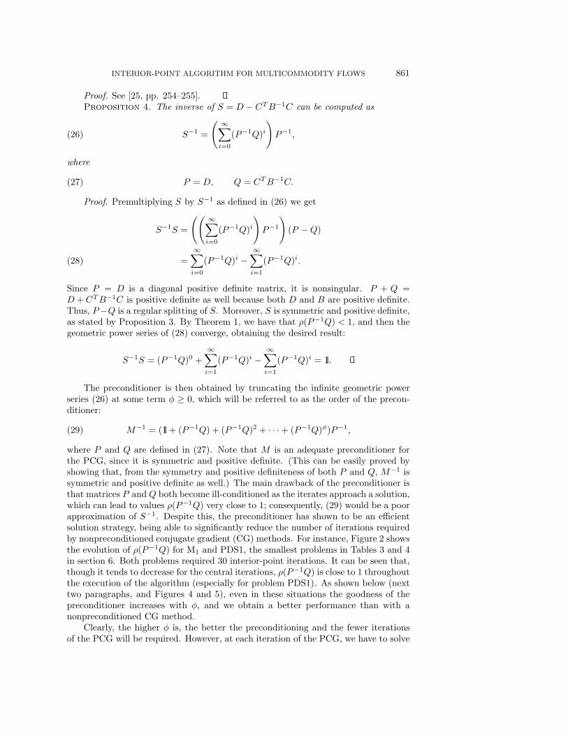
where P and Q are defined in (27). Note that M is an adequate preconditioner forthe PCG, since it is symmetric and positive definite. (This can be easily proved byshowing that, from the symmetry and positive definiteness of both P and Q, M−1 issymmetric and positive definite as well.) The main drawback of the preconditioner isthat matrices P and Q both become ill-conditioned as the iterates approach a solution,which can lead to values ρ(P−1Q) very close to 1; consequently, (29) would be a poorapproximation of S−1. Despite this, the preconditioner has shown to be an efficientsolution strategy, being able to significantly reduce the number of iterations requiredby nonpreconditioned conjugate gradient (CG) methods. For instance, Figure 2 showsthe evolution of ρ(P−1Q) for M1 and PDS1, the smallest problems in Tables 3 and 4in section 6. Both problems required 30 interior-point iterations. It can be seen that,though it tends to decrease for the central iterations, ρ(P−1Q) is close to 1 throughoutthe execution of the algorithm (especially for problem PDS1). As shown below (nexttwo paragraphs, and Figures 4 and 5), even in these situations the goodness of thepreconditioner increases with φ, and we obtain a better performance than with anonpreconditioned CG method.

Clearly, the higher φ is, the better the preconditioning and the fewer iterationsof the PCG will be required. However, at each iteration of the PCG, we have to solve

862 JORDI CASTRO

MPDS1

1

ρ (P

Q

)-1

0.88

0.9

0.92

0.94

0.96

0.98

1

0 5 10 15 20 25 30Iteration number

Fig. 2. Evolution of ρ(P−1Q) for the M1 and PDS1 problems.

Procedure MZ=r (P,Q, r, z, φ)

v := P−1r

z0 := v

for j=1 to φ do

zj := P−1Qzj−1 + v

end doz := zφ

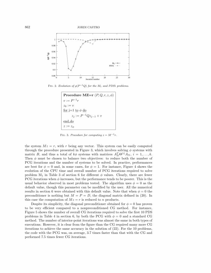
Fig. 3. Procedure for computing z = M−1r.

the system Mz = r, with r being any vector. This system can be easily computedthrough the procedure presented in Figure 3, which involves solving φ systems withmatrix B, and thus a total of kφ systems with matrices AT

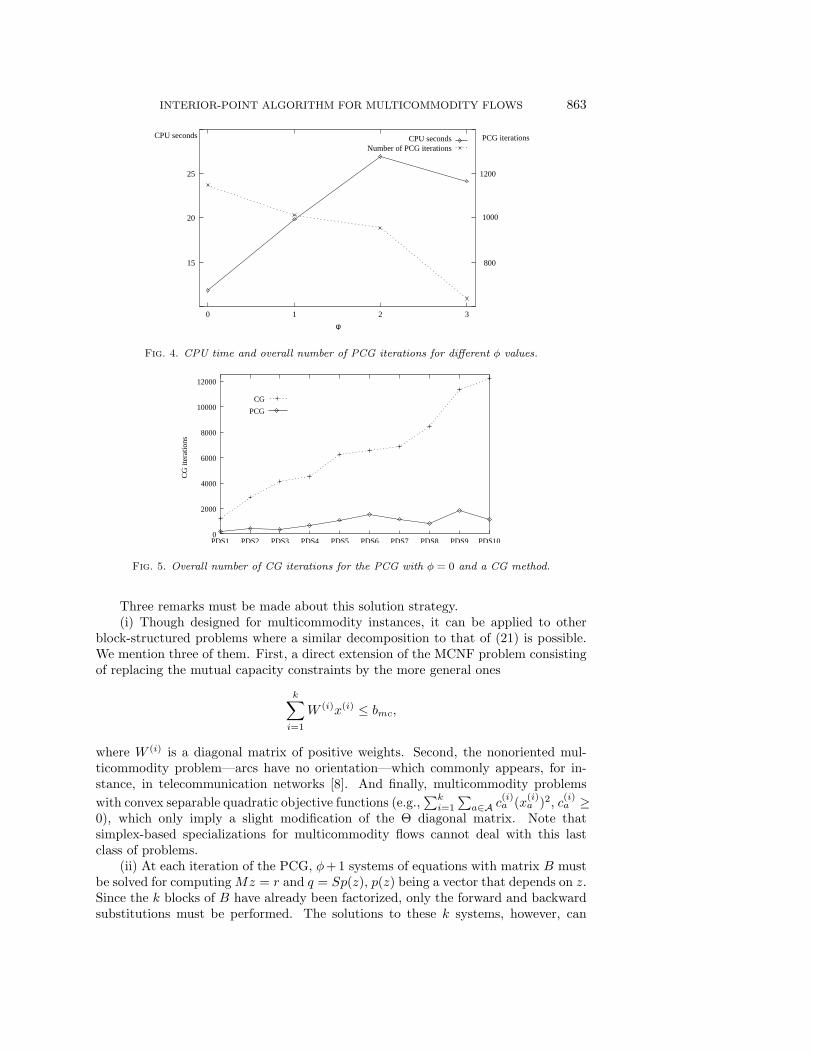
NΘ(i)AN , i = 1, . . . , k.Then φ must be chosen to balance two objectives: to reduce both the number ofPCG iterations and the number of systems to be solved. In practice, performancesare best for φ = 0 and, in some cases, for φ = 1. For instance, Figure 4 shows theevolution of the CPU time and overall number of PCG iterations required to solveproblem M1 in Table 3 of section 6 for different φ values. Clearly, there are fewerPCG iterations when φ increases, but the performance tends to be poorer. This is theusual behavior observed in most problems tested. The algorithm uses φ = 0 as thedefault value, though this parameter can be modified by the user. All the numericalresults in section 6 were obtained with this default value. Note that when φ = 0 thepreconditioner is nothing but M = P = D, the diagonal matrix defined in (20). Inthis case the computation of Mz = r is reduced to n products.

Despite its simplicity, the diagonal preconditioner obtained for φ = 0 has provento be very efficient compared to a nonpreconditioned CG method. For instance,Figure 5 shows the number of overall CG iterations required to solve the first 10 PDSproblems in Table 4 in section 6, by both the PCG with φ = 0 and a standard CGmethod. The number of interior-point iterations was almost the same in both types ofexecutions. However, it is clear from the figure than the CG required many more CGiterations to achieve the same accuracy in the solution of (22). For the 10 problems,the code with the PCG was, on average, 3.7 times faster than that with the CG andperformed 7.5 times fewer CG iterations.


15

20

25

0 1 3

Number of PCG iterationsCPU seconds

2

800

1200

1000

CPU seconds

φ

PCG iterations

Fig. 4. CPU time and overall number of PCG iterations for different φ values.

PCG

CG

0

2000

4000

6000

8000

10000

12000

PDS3 PDS6

CG

iter

atio

ns

PDS2 PDS4 PDS5 PDS7 PDS8 PDS9 PDS10PDS1

Fig. 5. Overall number of CG iterations for the PCG with φ = 0 and a CG method.

Three remarks must be made about this solution strategy.(i) Though designed for multicommodity instances, it can be applied to other

block-structured problems where a similar decomposition to that of (21) is possible.We mention three of them. First, a direct extension of the MCNF problem consistingof replacing the mutual capacity constraints by the more general ones

k∑

i=1

W (i)x(i) ≤ bmc,

where W (i) is a diagonal matrix of positive weights. Second, the nonoriented mul-ticommodity problem—arcs have no orientation—which commonly appears, for in-stance, in telecommunication networks [8]. And finally, multicommodity problemswith convex separable quadratic objective functions (e.g.,

∑ki=1

∑a∈A c

(i)a (x(i)

a )2, c(i)a ≥

0), which only imply a slight modification of the Θ diagonal matrix. Note thatsimplex-based specializations for multicommodity flows cannot deal with this lastclass of problems.

(ii) At each iteration of the PCG, φ+1 systems of equations with matrix B mustbe solved for computing Mz = r and q = Sp(z), p(z) being a vector that depends on z.Since the k blocks of B have already been factorized, only the forward and backwardsubstitutions must be performed. The solutions to these k systems, however, can

864 JORDI CASTRO

0.1

1

10

0 100 200 300 400 500 600

Number of variables (*1000)

CPU time ratioCG iterations ratioIP iterations ratio

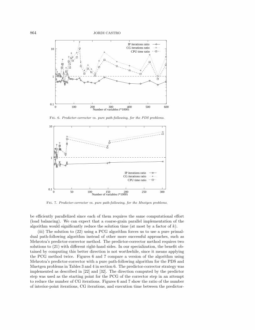
Fig. 6. Predictor-corrector vs. pure path-following, for the PDS problems.

CPU time ratioCG iterations ratioIP iterations ratio

0.1

1

10

0 50 100 150 200 250 300Number of variables (*1000)

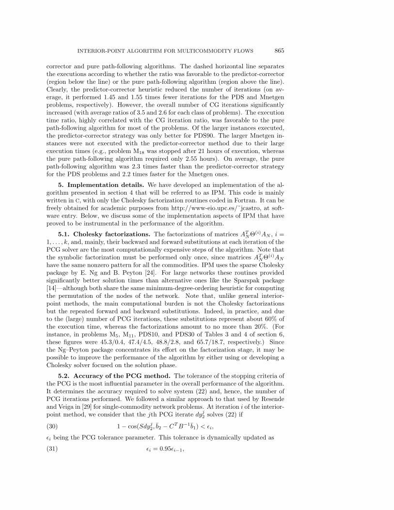
Fig. 7. Predictor-corrector vs. pure path-following, for the Mnetgen problems.

be efficiently parallelized since each of them requires the same computational effort(load balancing). We can expect that a coarse-grain parallel implementation of thealgorithm would significantly reduce the solution time (at most by a factor of k).

(iii) The solution to (22) using a PCG algorithm forces us to use a pure primal-dual path-following algorithm instead of other more successful approaches, such asMehrotra’s predictor-corrector method. The predictor-corrector method requires twosolutions to (21) with different right-hand sides. In our specialization, the benefit ob-tained by computing this better direction is not worthwhile, since it means applyingthe PCG method twice. Figures 6 and 7 compare a version of the algorithm usingMehrotra’s predictor-corrector with a pure path-following algorithm for the PDS andMnetgen problems in Tables 3 and 4 in section 6. The predictor-corrector strategy wasimplemented as described in [22] and [32]. The direction computed by the predictorstep was used as the starting point for the PCG of the corrector step in an attemptto reduce the number of CG iterations. Figures 6 and 7 show the ratio of the numberof interior-point iterations, CG iterations, and execution time between the predictor-


corrector and pure path-following algorithms. The dashed horizontal line separatesthe executions according to whether the ratio was favorable to the predictor-corrector(region below the line) or the pure path-following algorithm (region above the line).Clearly, the predictor-corrector heuristic reduced the number of iterations (on av-erage, it performed 1.45 and 1.55 times fewer iterations for the PDS and Mnetgenproblems, respectively). However, the overall number of CG iterations significantlyincreased (with average ratios of 3.5 and 2.6 for each class of problems). The executiontime ratio, highly correlated with the CG iteration ratio, was favorable to the purepath-following algorithm for most of the problems. Of the larger instances executed,the predictor-corrector strategy was only better for PDS90. The larger Mnetgen in-stances were not executed with the predictor-corrector method due to their largeexecution times (e.g., problem M18 was stopped after 21 hours of execution, whereasthe pure path-following algorithm required only 2.55 hours). On average, the purepath-following algorithm was 2.3 times faster than the predictor-corrector strategyfor the PDS problems and 2.2 times faster for the Mnetgen ones.

5. Implementation details. We have developed an implementation of the al-gorithm presented in section 4 that will be referred to as IPM. This code is mainlywritten in C, with only the Cholesky factorization routines coded in Fortran. It can befreely obtained for academic purposes from http://www-eio.upc.es/˜jcastro, at soft-ware entry. Below, we discuss some of the implementation aspects of IPM that haveproved to be instrumental in the performance of the algorithm.

5.1. Cholesky factorizations. The factorizations of matrices ATNΘ(i)AN , i =

1, . . . , k, and, mainly, their backward and forward substitutions at each iteration of thePCG solver are the most computationally expensive steps of the algorithm. Note thatthe symbolic factorization must be performed only once, since matrices AT

NΘ(i)AN

have the same nonzero pattern for all the commodities. IPM uses the sparse Choleskypackage by E. Ng and B. Peyton [24]. For large networks these routines providedsignificantly better solution times than alternative ones like the Sparspak package[14]—although both share the same minimum-degree-ordering heuristic for computingthe permutation of the nodes of the network. Note that, unlike general interior-point methods, the main computational burden is not the Cholesky factorizationsbut the repeated forward and backward substitutions. Indeed, in practice, and dueto the (large) number of PCG iterations, these substitutions represent about 60% ofthe execution time, whereas the factorizations amount to no more than 20%. (Forinstance, in problems M5, M11, PDS10, and PDS30 of Tables 3 and 4 of section 6,these figures were 45.3/0.4, 47.4/4.5, 48.8/2.8, and 65.7/18.7, respectively.) Sincethe Ng–Peyton package concentrates its effort on the factorization stage, it may bepossible to improve the performance of the algorithm by either using or developing aCholesky solver focused on the solution phase.

5.2. Accuracy of the PCG method. The tolerance of the stopping criteria ofthe PCG is the most influential parameter in the overall performance of the algorithm.It determines the accuracy required to solve system (22) and, hence, the number ofPCG iterations performed. We followed a similar approach to that used by Resendeand Veiga in [29] for single-commodity network problems. At iteration i of the interior-point method, we consider that the jth PCG iterate dyj

2 solves (22) if

1− cos(Sdyj2, b2 − CT B−1b1) < εi,(30)

εi being the PCG tolerance parameter. This tolerance is dynamically updated as

εi = 0.95εi−1,(31)

866 JORDI CASTRO

0.5

1

1.5

2

2.5

1.0e-2 1.0e-3 1.0e-4 1.0e-5 1.0e-6ε0

Number of iterationsCPU time

Number of PCG iterations

rela

tive

valu

es to

bas

e ca

se 1

.0e-

2

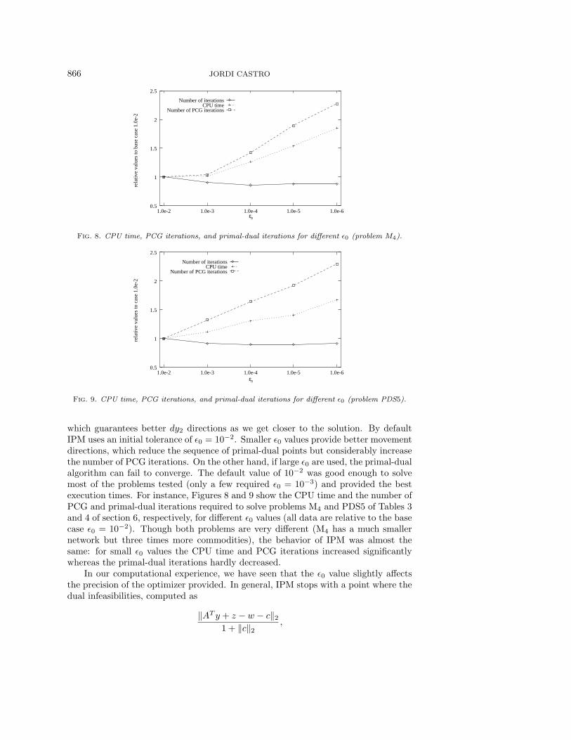
Fig. 8. CPU time, PCG iterations, and primal-dual iterations for different ε0 (problem M4).

ε0

0.5

1

1.5

2

2.5

1.0e-2 1.0e-3 1.0e-4 1.0e-5 1.0e-6

rela

tive

valu

es to

cas

e 1.

0e-2

Number of iterationsCPU time

Number of PCG iterations

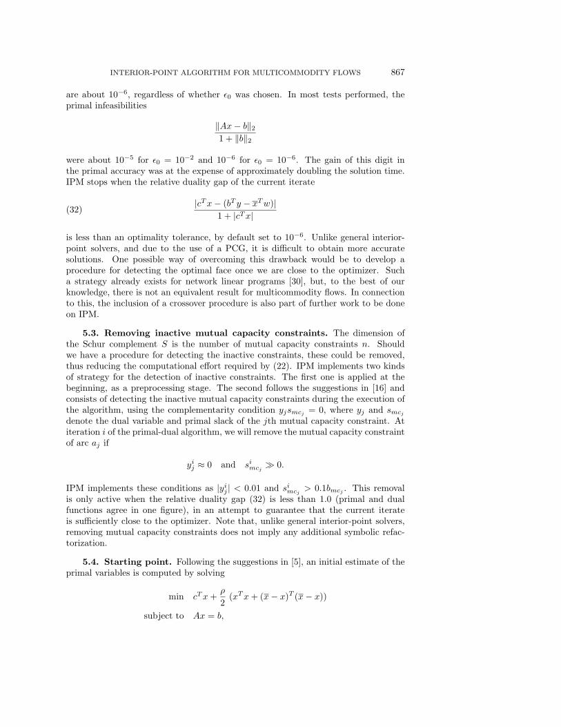
Fig. 9. CPU time, PCG iterations, and primal-dual iterations for different ε0 (problem PDS5).

which guarantees better dy2 directions as we get closer to the solution. By defaultIPM uses an initial tolerance of ε0 = 10−2. Smaller ε0 values provide better movementdirections, which reduce the sequence of primal-dual points but considerably increasethe number of PCG iterations. On the other hand, if large ε0 are used, the primal-dualalgorithm can fail to converge. The default value of 10−2 was good enough to solvemost of the problems tested (only a few required ε0 = 10−3) and provided the bestexecution times. For instance, Figures 8 and 9 show the CPU time and the number ofPCG and primal-dual iterations required to solve problems M4 and PDS5 of Tables 3and 4 of section 6, respectively, for different ε0 values (all data are relative to the basecase ε0 = 10−2). Though both problems are very different (M4 has a much smallernetwork but three times more commodities), the behavior of IPM was almost thesame: for small ε0 values the CPU time and PCG iterations increased significantlywhereas the primal-dual iterations hardly decreased.

In our computational experience, we have seen that the ε0 value slightly affectsthe precision of the optimizer provided. In general, IPM stops with a point where thedual infeasibilities, computed as

‖AT y + z − w − c‖21 + ‖c‖2 ,


are about 10−6, regardless of whether ε0 was chosen. In most tests performed, theprimal infeasibilities

‖Ax− b‖21 + ‖b‖2

were about 10−5 for ε0 = 10−2 and 10−6 for ε0 = 10−6. The gain of this digit inthe primal accuracy was at the expense of approximately doubling the solution time.IPM stops when the relative duality gap of the current iterate

|cT x− (bT y − xT w)|1 + |cT x|(32)

is less than an optimality tolerance, by default set to 10−6. Unlike general interior-point solvers, and due to the use of a PCG, it is difficult to obtain more accuratesolutions. One possible way of overcoming this drawback would be to develop aprocedure for detecting the optimal face once we are close to the optimizer. Sucha strategy already exists for network linear programs [30], but, to the best of ourknowledge, there is not an equivalent result for multicommodity flows. In connectionto this, the inclusion of a crossover procedure is also part of further work to be doneon IPM.

5.3. Removing inactive mutual capacity constraints. The dimension ofthe Schur complement S is the number of mutual capacity constraints n. Shouldwe have a procedure for detecting the inactive constraints, these could be removed,thus reducing the computational effort required by (22). IPM implements two kindsof strategy for the detection of inactive constraints. The first one is applied at thebeginning, as a preprocessing stage. The second follows the suggestions in [16] andconsists of detecting the inactive mutual capacity constraints during the execution ofthe algorithm, using the complementarity condition yjsmcj = 0, where yj and smcj

denote the dual variable and primal slack of the jth mutual capacity constraint. Atiteration i of the primal-dual algorithm, we will remove the mutual capacity constraintof arc aj if

yij ≈ 0 and si

mcjÀ 0.

IPM implements these conditions as |yij | < 0.01 and si

mcj> 0.1bmcj . This removal

is only active when the relative duality gap (32) is less than 1.0 (primal and dualfunctions agree in one figure), in an attempt to guarantee that the current iterateis sufficiently close to the optimizer. Note that, unlike general interior-point solvers,removing mutual capacity constraints does not imply any additional symbolic refac-torization.

5.4. Starting point. Following the suggestions in [5], an initial estimate of theprimal variables is computed by solving

min cT x +ρ

2(xT x + (x− x)T (x− x))

subject to Ax = b,

868 JORDI CASTRO

with |ρ| = 100, yielding

λ = (AAT )−1

(b

2ρ+ A

(c− x

ρ

)),

x =12

(x +

AT λ− c

ρ

).

Thereafter, the components xi out of bounds are replaced by min{xi/2, 100}.Dual estimators are obtained from the dual feasibility and complementarity slack-

ness conditions

(AT y)i + zi − wi = ci,

xizi = µ0,(33)

(xi − xi)wi = µ0,

where µ0 is set to a large value (e.g., 100). Dual variables are initialized as y = 0.Dual slacks are computed from (33), yielding

zi =µ0

xi+

ci

2+

√µ2

0

x2i

+c2i

4,

wi =µ0zi

xizi − µ0.

Note that for µ0 > 0 the above equations provide strictly positive values for w and z.

6. Computational results. To test the performance of the algorithm, IPM hasbeen compared with the NetOpt routine of CPLEX 4.0 [10] (which uses the solutionto k minimum-cost network problems, one for each commodity, as a warm start ofa dual simplex solver), and with PPRN [6], a primal partitioning code for linearand nonlinear multicommodity flows. For all the three codes, we used the defaulttolerances. All runs were carried out on a Sun/Ultra2 2200 workstation with 200MHz clock, 256 Mbytes of main memory, ≈68 Mflops Linpack, 14.7 Specfp95, and 7.8Specint95.

For the comparison, we considered three kinds of problem. The first one was ob-tained from the meta-generator Dimacs2pprn (see [6]). This meta-generator requires aprevious minimum-cost network flow problem that is converted to a multicommodityone. It can be obtained from ftp://ftp-eio.upc.es/pub/onl/codes/pprn/tests (an en-hanced version is described in [13]). We used four minimum-cost network generatorsfrom the DIMACS suite [11]: Rmfgen (D. Goldfarb and M. Grigoriadis), Grid-on-Torus (A. V. Goldberg), Gridgraph (M. G. C. Resende), and Gridgen (Y. Lee andJ. Orlin). They are freely distributed and can be obtained via anonymous ftp fromdimacs.rutgers.edu at directory /pub/netflow. We generated two kinds of problem foreach generator: with few commodities (small problems) and with many commodities(large problems). The small problems are represented by Si

k, where i = 1, . . . , 4 de-notes the DIMACS generator used (1 = Rmfgen, 2 = Grid-on-Torus, 3 = Gridgraph,4 = Gridgen) and k ∈ {1, 4, 8, 16, 50, 100, 150, 200} is the number of commodities con-sidered. The large problems are called Li

k, where i and k have the same meaning as


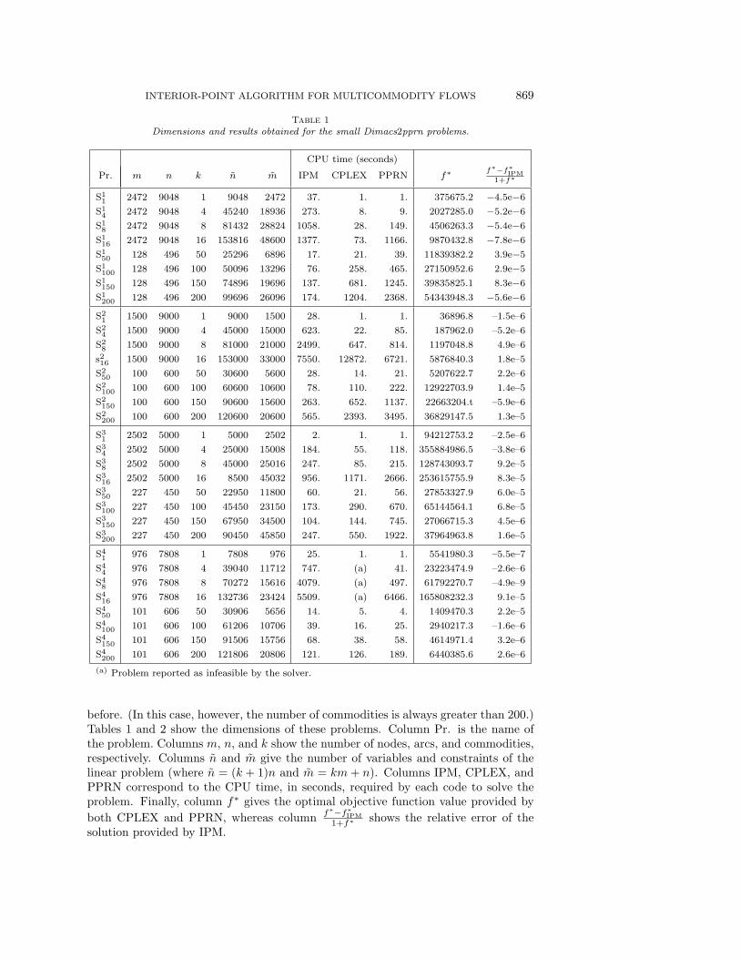
Table 1Dimensions and results obtained for the small Dimacs2pprn problems.

CPU time (seconds)

Pr. m n k n m IPM CPLEX PPRN f∗ f∗−f∗IPM1+f∗

S11 2472 9048 1 9048 2472 37. 1. 1. 375675.2 −4.5e−6

S14 2472 9048 4 45240 18936 273. 8. 9. 2027285.0 −5.2e−6

S18 2472 9048 8 81432 28824 1058. 28. 149. 4506263.3 −5.4e−6

S116 2472 9048 16 153816 48600 1377. 73. 1166. 9870432.8 −7.8e−6

S150 128 496 50 25296 6896 17. 21. 39. 11839382.2 3.9e−5

S1100 128 496 100 50096 13296 76. 258. 465. 27150952.6 2.9e−5

S1150 128 496 150 74896 19696 137. 681. 1245. 39835825.1 8.3e−6

S1200 128 496 200 99696 26096 174. 1204. 2368. 54343948.3 −5.6e−6

S21 1500 9000 1 9000 1500 28. 1. 1. 36896.8 –1.5e–6

S24 1500 9000 4 45000 15000 623. 22. 85. 187962.0 –5.2e–6

S28 1500 9000 8 81000 21000 2499. 647. 814. 1197048.8 4.9e–6

s216 1500 9000 16 153000 33000 7550. 12872. 6721. 5876840.3 1.8e–5

S250 100 600 50 30600 5600 28. 14. 21. 5207622.7 2.2e–6

S2100 100 600 100 60600 10600 78. 110. 222. 12922703.9 1.4e–5

S2150 100 600 150 90600 15600 263. 652. 1137. 22663204.t –5.9e–6

S2200 100 600 200 120600 20600 565. 2393. 3495. 36829147.5 1.3e–5

S31 2502 5000 1 5000 2502 2. 1. 1. 94212753.2 –2.5e–6

S34 2502 5000 4 25000 15008 184. 55. 118. 355884986.5 –3.8e–6

S38 2502 5000 8 45000 25016 247. 85. 215. 128743093.7 9.2e–5

S316 2502 5000 16 8500 45032 956. 1171. 2666. 253615755.9 8.3e–5

S350 227 450 50 22950 11800 60. 21. 56. 27853327.9 6.0e–5

S3100 227 450 100 45450 23150 173. 290. 670. 65144564.1 6.8e–5

S3150 227 450 150 67950 34500 104. 144. 745. 27066715.3 4.5e–6

S3200 227 450 200 90450 45850 247. 550. 1922. 37964963.8 1.6e–5

S41 976 7808 1 7808 976 25. 1. 1. 5541980.3 –5.5e–7

S44 976 7808 4 39040 11712 747. (a) 41. 23223474.9 –2.6e–6

S48 976 7808 8 70272 15616 4079. (a) 497. 61792270.7 –4.9e–9

S416 976 7808 16 132736 23424 5509. (a) 6466. 165808232.3 9.1e–5

S450 101 606 50 30906 5656 14. 5. 4. 1409470.3 2.2e–5

S4100 101 606 100 61206 10706 39. 16. 25. 2940217.3 –1.6e–6

S4150 101 606 150 91506 15756 68. 38. 58. 4614971.4 3.2e–6

S4200 101 606 200 121806 20806 121. 126. 189. 6440385.6 2.6e–6

(a) Problem reported as infeasible by the solver.

before. (In this case, however, the number of commodities is always greater than 200.)Tables 1 and 2 show the dimensions of these problems. Column Pr. is the name ofthe problem. Columns m, n, and k show the number of nodes, arcs, and commodities,respectively. Columns n and m give the number of variables and constraints of thelinear problem (where n = (k + 1)n and m = km + n). Columns IPM, CPLEX, andPPRN correspond to the CPU time, in seconds, required by each code to solve theproblem. Finally, column f∗ gives the optimal objective function value provided byboth CPLEX and PPRN, whereas column f∗−f∗IPM

1+f∗ shows the relative error of thesolution provided by IPM.

870 JORDI CASTRO

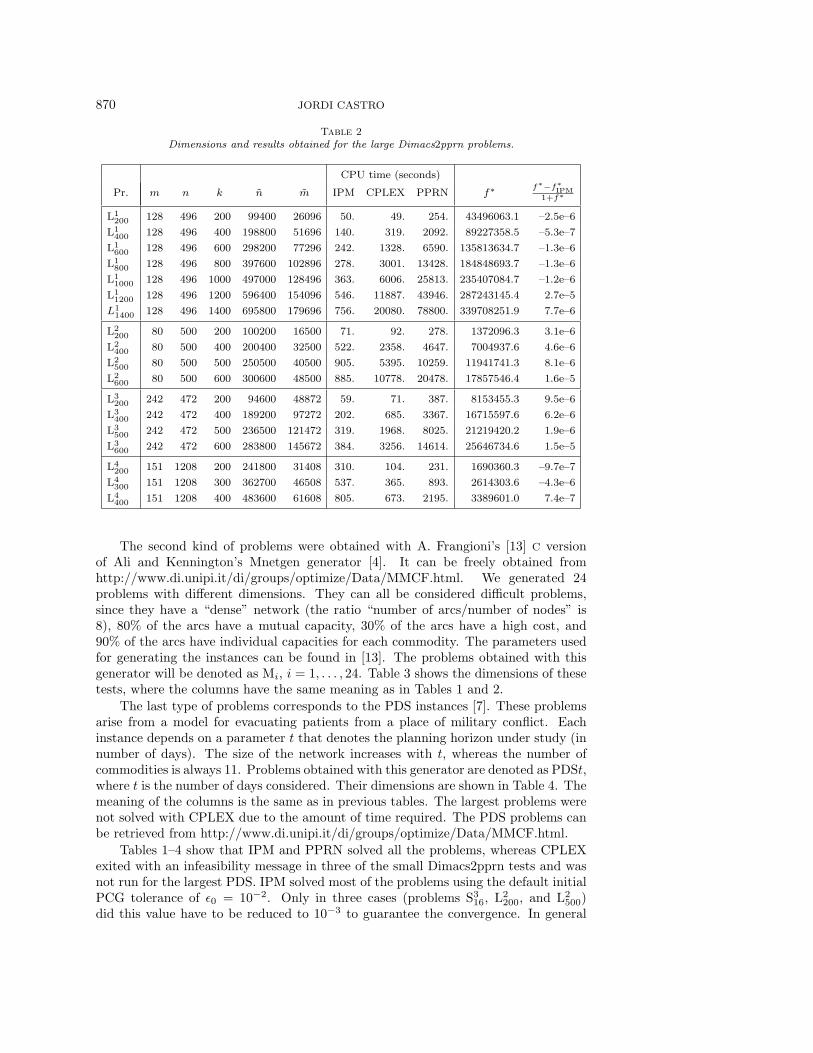
Table 2Dimensions and results obtained for the large Dimacs2pprn problems.

CPU time (seconds)


L1200 128 496 200 99400 26096 50. 49. 254. 43496063.1 –2.5e–6

L1400 128 496 400 198800 51696 140. 319. 2092. 89227358.5 –5.3e–7

L1600 128 496 600 298200 77296 242. 1328. 6590. 135813634.7 –1.3e–6

L1800 128 496 800 397600 102896 278. 3001. 13428. 184848693.7 –1.3e–6

L11000 128 496 1000 497000 128496 363. 6006. 25813. 235407084.7 –1.2e–6

L11200 128 496 1200 596400 154096 546. 11887. 43946. 287243145.4 2.7e–5

L11400 128 496 1400 695800 179696 756. 20080. 78800. 339708251.9 7.7e–6

L2200 80 500 200 100200 16500 71. 92. 278. 1372096.3 3.1e–6

L2400 80 500 400 200400 32500 522. 2358. 4647. 7004937.6 4.6e–6

L2500 80 500 500 250500 40500 905. 5395. 10259. 11941741.3 8.1e–6

L2600 80 500 600 300600 48500 885. 10778. 20478. 17857546.4 1.6e–5

L3200 242 472 200 94600 48872 59. 71. 387. 8153455.3 9.5e–6

L3400 242 472 400 189200 97272 202. 685. 3367. 16715597.6 6.2e–6

L3500 242 472 500 236500 121472 319. 1968. 8025. 21219420.2 1.9e–6

L3600 242 472 600 283800 145672 384. 3256. 14614. 25646734.6 1.5e–5

L4200 151 1208 200 241800 31408 310. 104. 231. 1690360.3 –9.7e–7

L4300 151 1208 300 362700 46508 537. 365. 893. 2614303.6 –4.3e–6

L4400 151 1208 400 483600 61608 805. 673. 2195. 3389601.0 7.4e–7

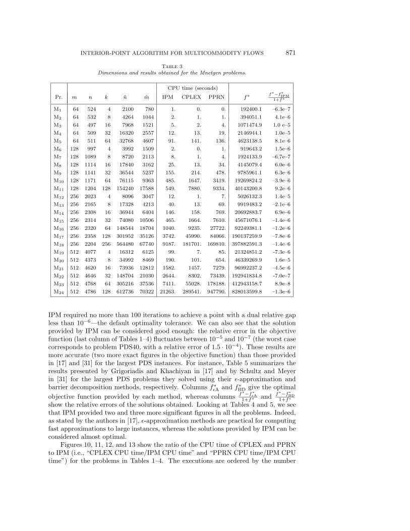
The second kind of problems were obtained with A. Frangioni’s [13] C versionof Ali and Kennington’s Mnetgen generator [4]. It can be freely obtained fromhttp://www.di.unipi.it/di/groups/optimize/Data/MMCF.html. We generated 24problems with different dimensions. They can all be considered difficult problems,since they have a “dense” network (the ratio “number of arcs/number of nodes” is8), 80% of the arcs have a mutual capacity, 30% of the arcs have a high cost, and90% of the arcs have individual capacities for each commodity. The parameters usedfor generating the instances can be found in [13]. The problems obtained with thisgenerator will be denoted as Mi, i = 1, . . . , 24. Table 3 shows the dimensions of thesetests, where the columns have the same meaning as in Tables 1 and 2.

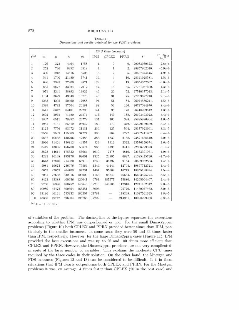
The last type of problems corresponds to the PDS instances [7]. These problemsarise from a model for evacuating patients from a place of military conflict. Eachinstance depends on a parameter t that denotes the planning horizon under study (innumber of days). The size of the network increases with t, whereas the number ofcommodities is always 11. Problems obtained with this generator are denoted as PDSt,where t is the number of days considered. Their dimensions are shown in Table 4. Themeaning of the columns is the same as in previous tables. The largest problems werenot solved with CPLEX due to the amount of time required. The PDS problems canbe retrieved from http://www.di.unipi.it/di/groups/optimize/Data/MMCF.html.

Tables 1–4 show that IPM and PPRN solved all the problems, whereas CPLEXexited with an infeasibility message in three of the small Dimacs2pprn tests and wasnot run for the largest PDS. IPM solved most of the problems using the default initialPCG tolerance of ε0 = 10−2. Only in three cases (problems S3

16, L2200, and L2

500)did this value have to be reduced to 10−3 to guarantee the convergence. In general


Table 3Dimensions and results obtained for the Mnetgen problems.

CPU time (seconds)


M1 64 524 4 2100 780 1. 0. 0. 192400.1 –6.3e–7

M2 64 532 8 4264 1044 2. 1. 1. 394051.1 4.1e–6

M3 64 497 16 7968 1521 5. 2. 4. 1071474.9 1.0 e–5

M4 64 509 32 16320 2557 12. 13. 19. 2146944.1 1.0e–5

M5 64 511 64 32768 4607 91. 141. 136. 4623138.5 8.1e–6

M6 128 997 4 3992 1509 2. 0. 1. 919643.2 1.5e–6

M7 128 1089 8 8720 2113 8. 1. 4. 1924133.9 –6.7e–7

M8 128 1114 16 17840 3162 25. 13. 34. 4145079.4 6.0e–6

M9 128 1141 32 36544 5237 155. 214. 478. 9785961.1 6.3e–6

M10 128 1171 64 76115 9363 485. 1647. 3419. 19269824.2 –3.9e–6

M11 128 1204 128 154240 17588 549. 7880. 9334. 40143200.8 9.2e–6

M12 256 2023 4 8096 3047 12. 1. 7. 5026132.3 1.4e–5

M13 256 2165 8 17328 4213 40. 13. 69. 9919483.2 –2.1e–6

M14 256 2308 16 36944 6404 146. 158. 769. 20692883.7 6.9e–6

M15 256 2314 32 74080 10506 465. 1664. 7610. 45671076.1 –1.4e–6

M16 256 2320 64 148544 18704 1040. 9235. 27722. 92249381.1 –1.2e–6

M17 256 2358 128 301952 35126 3742. 45990. 84066. 190137259.9 –7.8e–6

M18 256 2204 256 564480 67740 9187. 181701. 169810. 397882591.3 –1.4e–6

M19 512 4077 4 16312 6125 99. 7. 85. 21324851.2 -7.3e–6

M20 512 4373 8 34992 8469 190. 101. 654. 46339269.9 1.6e–5

M21 512 4620 16 73936 12812 1582. 1457. 7279. 96992237.2 –4.5e–6

M22 512 4646 32 148704 21030 2644. 8302. 73439. 192941834.8 -7.0e–7

M23 512 4768 64 305216 37536 7411. 55028. 178188. 412943158.7 8.9e–8

M24 512 4786 128 612736 70322 21263. 289541. 947790. 828013599.8 –1.3e–6

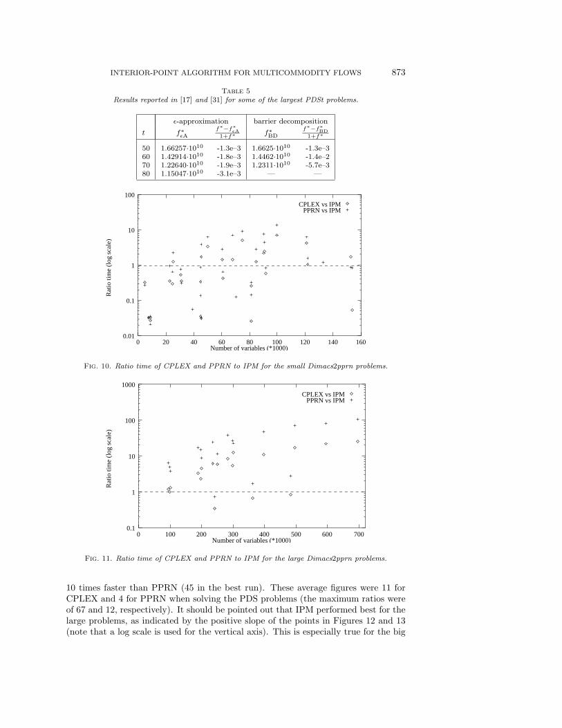
IPM required no more than 100 iterations to achieve a point with a dual relative gapless than 10−6—the default optimality tolerance. We can also see that the solutionprovided by IPM can be considered good enough: the relative error in the objectivefunction (last column of Tables 1–4) fluctuates between 10−5 and 10−7 (the worst casecorresponds to problem PDS40, with a relative error of 1.5 · 10−4). These results aremore accurate (two more exact figures in the objective function) than those providedin [17] and [31] for the largest PDS instances. For instance, Table 5 summarizes theresults presented by Grigoriadis and Khachiyan in [17] and by Schultz and Meyerin [31] for the largest PDS problems they solved using their ε-approximation andbarrier decomposition methods, respectively. Columns f∗εA and f∗BD give the optimalobjective function provided by each method, whereas columns f∗−f∗εA

1+f∗ and f∗−f∗BD1+f∗

show the relative errors of the solutions obtained. Looking at Tables 4 and 5, we seethat IPM provided two and three more significant figures in all the problems. Indeed,as stated by the authors in [17], ε-approximation methods are practical for computingfast approximations to large instances, whereas the solutions provided by IPM can beconsidered almost optimal.

Figures 10, 11, 12, and 13 show the ratio of the CPU time of CPLEX and PPRNto IPM (i.e., “CPLEX CPU time/IPM CPU time” and “PPRN CPU time/IPM CPUtime”) for the problems in Tables 1–4. The executions are ordered by the number

872 JORDI CASTRO

Table 4Dimensions and results obtained for the PDSt problems.

CPU time (seconds)

t(a) m n n m IPM CPLEX PPRN f∗ f∗−f∗IPM1+f∗

1 126 372 4464 1758 1. 0. 0. 29083930523. 2.8e–6

2 252 746 8952 3518 4. 1. 2. 28857862010. –5.9e–6

3 390 1218 14616 5508 8. 2. 5. 28597374145. –4.9e–6

4 541 1790 21480 7741 16. 4. 10. 28341928581. –1.5e–6

5 686 2325 27900 9871 29. 8. 19. 28054052607. –6.6e–6

6 835 2827 33924 12012 47. 13. 35. 27761037600. 1.3e–5

7 971 3241 38892 13922 46. 20. 52. 27510377013. 2.1e–5

8 1104 3629 43548 15773 45. 31. 75. 27239627210. 2.1e–5

9 1253 4205 50460 17988 94. 51. 84. 26974586241. 1.5e–5

10 1399 4792 57504 20181 88. 56. 136. 26727094976. 8.4e–6

11 1541 5342 64101 22293 144. 98. 178. 26418289612. 1.3e–5

12 1692 5965 71580 24577 113. 143. 188. 26103493922. 7.4e–5

13 1837 6571 78852 26778 137. 160. 328. 25825886804. 4.6e–5

14 1981 7151 85812 28942 180. 270. 342. 25529159469. 3.4e–5

15 2125 7756 93072 31131 236. 425. 564. 25177923601. 3.3e–5

18 2558 9589 115068 37727 396. 864. 1227. 24332411902. 6.4e–6

20 2857 10858 130296 42285 386. 1830. 2138. 23821658640. 7.0e–5

21 2996 11401 136812 44357 529. 1912. 2322. 23576150674. 2.6e–5

24 3419 13065 156780 50674 963. 4393. 3411. 22856729593. 5.1e–7

27 3823 14611 175332 56664 1010. 7178. 4810. 22133391961. 1.9e–5

30 4223 16148 193776 62601 1325. 24905. 6827. 21385445736. –1.7e–6

33 4643 17840 214080 68913 1750. 35397. 9154. 20589962883. 1.4e–5

36 5081 19673 236076 75564 1346. 44144. 12704. 19857712721. 4.4e–5

40 5652 22059 264708 84231 1494. 95064. 16779. 18855198824. 1.5e–4

50 7031 27668 332016 105009 4166. 85840. 46664. 16603525724. 3.5e–5

60 8423 33388 400656 126041 6761. 387577. 75880. 14265904407. 2.4e–6

70 9750 38396 460752 145646 12210. 540606. 112310. 12241162812. 2.0e–5

80 10989 42472 509664 163351 13005. — 125770. 11469077462. 3.0e–5

90 12186 46161 553932 180207 21781. — 178248. 11087561635. 1.8e–5

100 13366 49742 596904 196768 17222. — 214961. 10928229968. 8.8e–5

(a) k = 11 for all t.

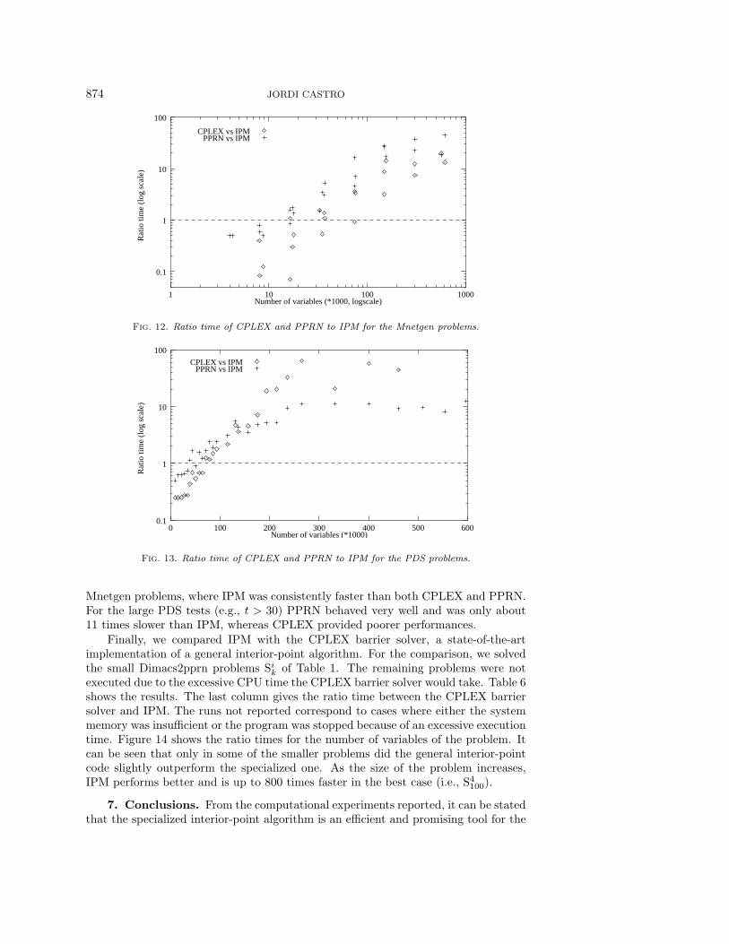
of variables of the problem. The dashed line of the figures separates the executionsaccording to whether IPM was outperformed or not. For the small Dimacs2pprnproblems (Figure 10) both CPLEX and PPRN provided better times than IPM, par-ticularly in the smaller instances. In some cases they were 50 and 33 times fasterthan IPM, respectively. However, for the large Dimacs2pprn cases (Figure 11), IPMprovided the best executions and was up to 26 and 100 times more efficient thanCPLEX and PPRN. However, the Dimacs2pprn problems are not very complicated,in spite of the large number of variables. This explains the moderate CPU timesrequired by the three codes in their solution. On the other hand, the Mnetgen andPDS instances (Figures 12 and 13) can be considered to be difficult. It is in thesesituations that IPM clearly outperforms both CPLEX and PPRN. For the Mnetgenproblems it was, on average, 4 times faster than CPLEX (20 in the best case) and


Table 5Results reported in [17] and [31] for some of the largest PDSt problems.

ε-approximation barrier decomposition

t f∗εAf∗−f∗εA1+f∗ f∗BD

f∗−f∗BD1+f∗

50 1.66257·1010 -1.3e–3 1.6625·1010 -1.3e–360 1.42914·1010 -1.8e–3 1.4462·1010 -1.4e–270 1.22640·1010 -1.9e–3 1.2311·1010 -5.7e–380 1.15047·1010 -3.1e–3 — —

0.01

0.1

1

10

100

0 20 40 60 80 100 120 140 160

Rat

io ti

me

(log

sca

le)


PPRN vs IPMCPLEX vs IPM

Fig. 10. Ratio time of CPLEX and PPRN to IPM for the small Dimacs2pprn problems.

0.1

1

10

100

1000

0 100 200 300 400 500 600 700Number of variables (*1000)

PPRN vs IPM

Rat

io ti

me

(log

sca

le)

CPLEX vs IPM

Fig. 11. Ratio time of CPLEX and PPRN to IPM for the large Dimacs2pprn problems.

10 times faster than PPRN (45 in the best run). These average figures were 11 forCPLEX and 4 for PPRN when solving the PDS problems (the maximum ratios wereof 67 and 12, respectively). It should be pointed out that IPM performed best for thelarge problems, as indicated by the positive slope of the points in Figures 12 and 13(note that a log scale is used for the vertical axis). This is especially true for the big

874 JORDI CASTRO

0.1

1

10

100

1 10 100 1000

Rat

io ti

me

(log

sca

le)

Number of variables (*1000, logscale)

PPRN vs IPMCPLEX vs IPM

Fig. 12. Ratio time of CPLEX and PPRN to IPM for the Mnetgen problems.

0.1

1

10

100

0 100 200 300 400 500 600

Rat

io ti

me

(log

sca

le)


CPLEX vs IPMPPRN vs IPM

Fig. 13. Ratio time of CPLEX and PPRN to IPM for the PDS problems.

Mnetgen problems, where IPM was consistently faster than both CPLEX and PPRN.For the large PDS tests (e.g., t > 30) PPRN behaved very well and was only about11 times slower than IPM, whereas CPLEX provided poorer performances.

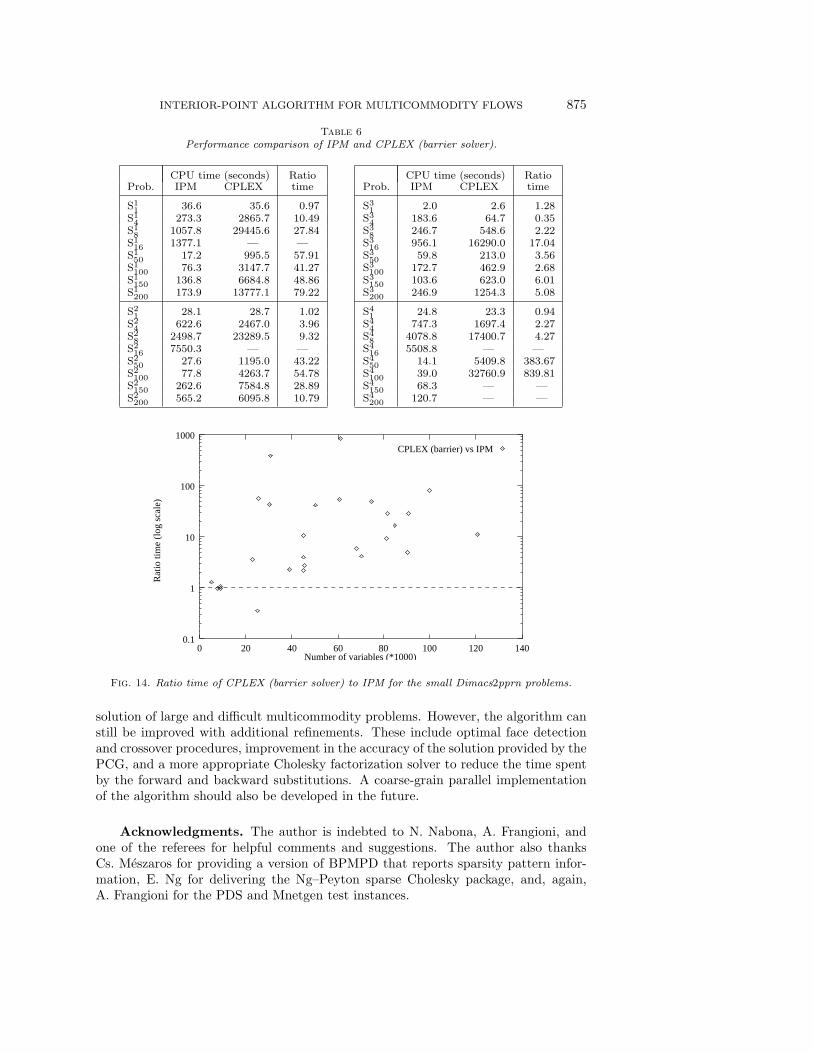
Finally, we compared IPM with the CPLEX barrier solver, a state-of-the-artimplementation of a general interior-point algorithm. For the comparison, we solvedthe small Dimacs2pprn problems Si

k of Table 1. The remaining problems were notexecuted due to the excessive CPU time the CPLEX barrier solver would take. Table 6shows the results. The last column gives the ratio time between the CPLEX barriersolver and IPM. The runs not reported correspond to cases where either the systemmemory was insufficient or the program was stopped because of an excessive executiontime. Figure 14 shows the ratio times for the number of variables of the problem. Itcan be seen that only in some of the smaller problems did the general interior-pointcode slightly outperform the specialized one. As the size of the problem increases,IPM performs better and is up to 800 times faster in the best case (i.e., S4

100).

7. Conclusions. From the computational experiments reported, it can be statedthat the specialized interior-point algorithm is an efficient and promising tool for the


Table 6Performance comparison of IPM and CPLEX (barrier solver).

CPU time (seconds) RatioProb. IPM CPLEX time

S11 36.6 35.6 0.97

S14 273.3 2865.7 10.49

S18 1057.8 29445.6 27.84

S116 1377.1 — —

S150 17.2 995.5 57.91

S1100 76.3 3147.7 41.27

S1150 136.8 6684.8 48.86

S1200 173.9 13777.1 79.22

S21 28.1 28.7 1.02

S24 622.6 2467.0 3.96

S28 2498.7 23289.5 9.32

S216 7550.3 — —

S250 27.6 1195.0 43.22

S2100 77.8 4263.7 54.78

S2150 262.6 7584.8 28.89

S2200 565.2 6095.8 10.79

CPU time (seconds) RatioProb. IPM CPLEX time

S31 2.0 2.6 1.28

S34 183.6 64.7 0.35

S38 246.7 548.6 2.22

S316 956.1 16290.0 17.04

S350 59.8 213.0 3.56

S3100 172.7 462.9 2.68

S3150 103.6 623.0 6.01

S3200 246.9 1254.3 5.08

S41 24.8 23.3 0.94

S44 747.3 1697.4 2.27

S48 4078.8 17400.7 4.27

S416 5508.8 — —

S450 14.1 5409.8 383.67

S4100 39.0 32760.9 839.81

S4150 68.3 — —

S4200 120.7 — —

0.1

1

10

100

1000

0 20 40 60 80 100 120 140

Rat

io ti

me

(log

sca

le)


CPLEX (barrier) vs IPM

Fig. 14. Ratio time of CPLEX (barrier solver) to IPM for the small Dimacs2pprn problems.

solution of large and difficult multicommodity problems. However, the algorithm canstill be improved with additional refinements. These include optimal face detectionand crossover procedures, improvement in the accuracy of the solution provided by thePCG, and a more appropriate Cholesky factorization solver to reduce the time spentby the forward and backward substitutions. A coarse-grain parallel implementationof the algorithm should also be developed in the future.

Acknowledgments. The author is indebted to N. Nabona, A. Frangioni, andone of the referees for helpful comments and suggestions. The author also thanksCs. Meszaros for providing a version of BPMPD that reports sparsity pattern infor-mation, E. Ng for delivering the Ng–Peyton sparse Cholesky package, and, again,A. Frangioni for the PDS and Mnetgen test instances.

876 JORDI CASTRO

REFERENCES

[1] I. Adler, M.G.C. Resende, and G. Veiga, An implementation of Karmarkar’s algorithm forlinear programming, Math. Programming, 44 (1989), pp. 297–335.

[2] R.K. Ahuja, T.L. Magnanti, and J.B. Orlin, Network Flows, Prentice-Hall, EnglewoodCliffs, NJ, 1993.

[3] A. Ali, R.V. Helgason, J.L. Kennington, and H. Lall, Computational comparison amongthree multicommodity network flow algorithms, Oper. Res., 28 (1980), pp. 995–1000.

[4] A. Ali and J.L. Kennington, Mnetgen Program Documentation, Technical Report 77003,Department of Industrial Engineering and Operations Research, Southern Methodist Uni-versity, Dallas, TX, 1977.

[5] E.D. Andersen, J. Gondzio, C. Meszaros, and X. Xu, Implementation of interior pointmethods for large scale linear programming, in Interior Point Methods in MathematicalProgramming, T. Terlaky, ed., Kluwer Academic Publishers, Dordrecht, The Netherlands,1996, pp. 189–252.

[6] J. Castro and N. Nabona, An implementation of linear and nonlinear multicommodity net-work flows, European J. Oper. Res., 92 (1996), pp. 37–53.

[7] W.J. Carolan, J.E. Hill, J.L. Kennington, S. Niemi, and S.J. Wichmann, An empiricalevaluation of the KORBX algorithms for military airlift applications, Oper. Res., 38 (1990),pp. 240–248.

[8] P. Chardaire and A. Lisser, Simplex and interior point specialized algorithms for solvingnon-oriented multicommodity flow problems, Oper. Res., accepted subject to revision.

[9] I.C. Choi and D. Goldfarb, Solving multicommodity network flow problems by an interiorpoint method, in Large-Scale Numerical Optimization, T.F. Coleman and Y. Li, eds., SIAM,Philadelphia, PA, 1990, pp. 58–69.

[10] CPLEX Optimization Inc., Using the CPLEX Callable Library, Incline Village, NV, 1995.[11] DIMACS, The First DIMACS International Algorithm Implementation Challenge: The

Benchmark Experiments, Technical Report, DIMACS, New Brunswick, NJ, 1991.[12] A. Frangioni, personal communication, Department of Computer Science, Universita di Pisa,

Pisa, Italy, 1998.[13] A. Frangioni and G. Gallo, A bundle type dual-ascent approach to linear multicommodity

min cost flow problems, INFORMS J. Comput., 11 (1999), pp. 370–393.[14] J.A. George and J.W. Liu, Computer Solution of Large Sparse Positive Definite Systems,

Prentice-Hall, Englewood Cliffs, NJ, 1981.[15] J.-L. Goffin, J. Gondzio, R. Sarkissian, and J.-P. Vial, Solving nonlinear multicommodity

flow problems by the analytic center cutting plane method, Math. Programming, 76 (1996),pp. 131–154.

[16] J. Gondzio and M. Makowski, Solving a class of LP problems with a primal-dual logarithmicbarrier method, European J. Oper. Res., 80 (1995), pp. 184–192.

[17] M.D. Grigoriadis and L.G. Khachiyan, An exponential-function reduction method for block-angular convex programs, Networks, 26 (1995), pp. 59–68.

[18] A.P. Kamath, N.K. Karmarkar, and K.G. Ramakrishnan, Computational and ComplexityResults for an Interior Point Algorithm on Multicommodity Flow Problems, TechnicalReport TR-21/93, Dip. di Informatica, Univ. di Pisa, Italy, 1993, pp. 116–122.

[19] A.P. Kamath and O. Palmon, Improved Interior Point Algorithms for Exact and Approxi-mate Solutions of Multicommodity Flow Problems, Technical Report, Dept. of ComputerSciences, Stanford University, Stanford, CA, 1994.

[20] S. Kapoor and P.M. Vaidya, Speeding up Karmarkar’s algorithm for multicommodity flows,Math. Programming, 73 (1996), pp. 111–127.

[21] J.L. Kennington and R.V. Helgason, Algorithms for Network Programming, Wiley, NewYork, 1980.

[22] I.J. Lustig, R.E. Marsten, and D.F. Shanno, On implementing Mehrotra’s predictor-corrector interior-point method for linear programming, SIAM J. Optim., 2 (1992), pp. 435–449.

[23] Cs. Meszaros, The Efficient Implementation of Interior Point Methods for Linear Program-ming and Their Applications, Ph.D. Thesis, Eotvos Lorand University of Sciences, Bu-dapest, Hungary, 1996.

[24] E. Ng and B.W. Peyton, Block sparse Cholesky algorithms on advanced uniprocessor com-puters, SIAM J. Sci. Comput., 14 (1993), pp. 1034–1056.

[25] J.M. Ortega, Introduction to Parallel and Vector Solution of Linear Systems, Plenum Press,New York, 1988.

[26] L. Portugal, M.G.C. Resende, G. Veiga, G., and J. Judice, A truncated primal-infeasible


dual-feasible network interior point method, Networks, 35 (2000), pp. 91–108.[27] L. Portugal, M.G.C. Resende, G. Veiga, G., and J. Judice, A truncated interior-point

method for the solution of minimum cost flow problems on an undirected multicommodityflow network, in Proceedings of the First Portuguese National Telecommunications Con-ference, Aveiro, Portugal, 1997, pp. 381–384 (in Portuguese).

[28] M.G.C. Resende and P. Pardalos, Interior point algorithms for network flow problems, inAdvances in Linear and Integer Programming, J.E. Beasley, ed., Oxford University Press,New York, 1996, pp. 149–189.

[29] M.G.C. Resende and G. Veiga, An implementation of the dual affine scaling algorithmfor minimum-cost flow on bipartite uncapacitated networks, SIAM J. Optim., 3 (1993),pp. 516–537.

[30] M.G.C. Resende, T. Tsuchiya, and G. Veiga, Identifying the optimal face of a network linearprogram with a globally convergent interior point method, in Large Scale Optimization:State of the Art, W. Hager, D. Hearn, and P. Pardalos, eds., Kluwer Academic Publishers,Dordrecht, The Netherlands, 1994, pp. 362–387.

[31] G.L. Schultz and R.R. Meyer, An interior point method for block angular optimization,SIAM J. Optim., 1 (1991), pp. 583–602.

[32] S.J. Wright, Primal-Dual Interior-Point Methods, SIAM, Philadelphia, PA, 1996.[33] S. Zenios, A smooth penalty function algorithm for network-structured problems, European J.

Oper. Res., 83 (1995), pp. 220–236.

Documents

A SPECIALIZED INTERIOR-POINT ALGORITHM FOR MULTICOMMODITY