MASTER THESIS: ECONOMETRICS & MANAGEMENT SCIENCESPECIALISATION: ECONOMETRICS

INTERGENERATIONAL TRANSMISSIONOF SKILLS AND OCCUPATIONAL

CHOICE USING STRUCTURALEQUATION MODELLING

August 2, 2021

ERASMUS UNIVERSITEIT ROTTERDAMErasmus School of Economics

Author: Aarthi S.IyerStudent ID number: 523320Supervisor: dr. AJ Koning

Second assessor: dr. O Kleen

Abstract

Development of skills by the youth can help address the issues of employment,entrepreneurship, improve economic, equitable and sustainable growth. Skills can becategorised into cognitive, non-cognitive and technical skills. This paper seeks to an-swer whether the occupation choice of an individual is influenced by the transmissionof skills from their parents or their occupation. Since these skills are unobserved vari-ables, the methodology used for answering the research question is Structural EquationModelling(SEM) which makes use of latent and observed variables. The results foundindicate that positive intergenerational transmission of cognitive skills which impactthe occupational choice of an individual. However, for non-cognitive skills, no evidenceof intergenerational transmission of skills from mother is found, but positive evidenceof influence of parental investment, self-productivity and cross-productivity is foundwhich impacts the occupational choice of an individual.

The content of this thesis is the sole responsibility of the author and does not reflect theview of the supervisor, Erasmus School of Economics or Erasmus University.

Contents

1 Introduction 4

2 Methodology 92.1 Measurement Model . . . . . . . . . . . . . . . . . . . . . . . . . . . . . . . 10

2.1.1 Confirmatory factor analysis . . . . . . . . . . . . . . . . . . . . . . . 112.2 Structural Model . . . . . . . . . . . . . . . . . . . . . . . . . . . . . . . . . 122.3 LISREL Illustrated Example . . . . . . . . . . . . . . . . . . . . . . . . . . . 12

3 Model 143.1 Part I: Measurement Model . . . . . . . . . . . . . . . . . . . . . . . . . . . 143.2 Part II: Structural Model . . . . . . . . . . . . . . . . . . . . . . . . . . . . . 153.3 Part III: Impact of skills on occupational choice . . . . . . . . . . . . . . . . 153.4 Identification of factor loadings . . . . . . . . . . . . . . . . . . . . . . . . . 15

4 Estimation 184.1 Estimation of measurement models . . . . . . . . . . . . . . . . . . . . . . . 184.2 Estimation of structural regression model . . . . . . . . . . . . . . . . . . . . 19

4.2.1 Bias Corrected factor score regression . . . . . . . . . . . . . . . . . . 204.3 Reliability of factors . . . . . . . . . . . . . . . . . . . . . . . . . . . . . . . 214.4 Goodness-of-fit indices . . . . . . . . . . . . . . . . . . . . . . . . . . . . . . 22

5 Data 25

6 Results 276.1 Summary Statistics . . . . . . . . . . . . . . . . . . . . . . . . . . . . . . . . 276.2 Part I: Measurement Model . . . . . . . . . . . . . . . . . . . . . . . . . . . 31

6.2.1 Reliability of factors . . . . . . . . . . . . . . . . . . . . . . . . . . . 376.2.2 Goodness-of-fit indices . . . . . . . . . . . . . . . . . . . . . . . . . . 38

6.3 Part II: Structural Model . . . . . . . . . . . . . . . . . . . . . . . . . . . . . 396.4 Part III: Estimation of occupational choice . . . . . . . . . . . . . . . . . . . 40

7 Discussion & Conclusion 41

References 43

8 Appendix 47

1 Introduction

In the labor market, workers are often classified as "White Collar" or "Blue Collar" workerswhich helps in understanding the social standing of the person, approach to life, life choicesamong others. This classification also tells about the kind of skill the individual possesswhich in turn determine their success in the labor market. The heterogeneity in the labormarket can be classified into two types, namely, labor services defined in terms of differ-ent knowledge, tasks, output or equipment, and in terms of individuals who supply laborin the market. Economic theory recognises that individual exhibit differences in both theirproductive capabilities and their preference for varieties of utility and disutility associatedwith supply of labor. Because of which individuals are not expected to suit each role andthese differences contribute to determinants of individual’s occupational outcomes, therebychoosing varied labor market roles (Ham et al., 2009b). One of the important factors con-tributing to the country’s economic growth and positive outlook is when it achieves increasedemployability along with labor productivity which can be attained if a worker achieves pro-ductivity by working towards their full working potential. With global changing trends suchas technological advancements, climate change and urbanization, the skills needed are evolv-ing continuously and rapidly. In this ever changing environment, the skills in high demandare cognitive skills such as critical thinking and problem solving, and socio-economic skillssuch as leadership, teamwork and grit along with relevant technical skills. Due to the pres-ence of heterogeneity in the labor market, breaking down the job roles into the requiredskill set can allow employers to understand viable job transition pathways and at the sametime also allow the employers to make decisions regarding reskilling or upskilling requiredfor such transitions (World Economic Forum, 2021). However, the labor market especiallyin developing countries workers are not able to reach their full working potential due to lowskills levels which is partly due to low education levels or due to skill mismatch. Such alack of skilled workers has limited the innovation that stems for employers and also affectsa country’s economic growth. Reskilling of workers or matching their skill with respectiveoccupation can help in alleviating the problem of skill mismatch highlighting the problem ofoccupational choice of an individual.

There are multiple sources of heterogeneity affecting the labor market, one of them identi-fied is human capital between individuals. Becker (2009) argues that there are diverse arrayof factors such as education level, on the job skill training, and experience which can beseen as investments in human capital increasing the productivity of an individual, thoughthe effects of education may have non-linear effects over the years (Heckman et al., 2003).

4

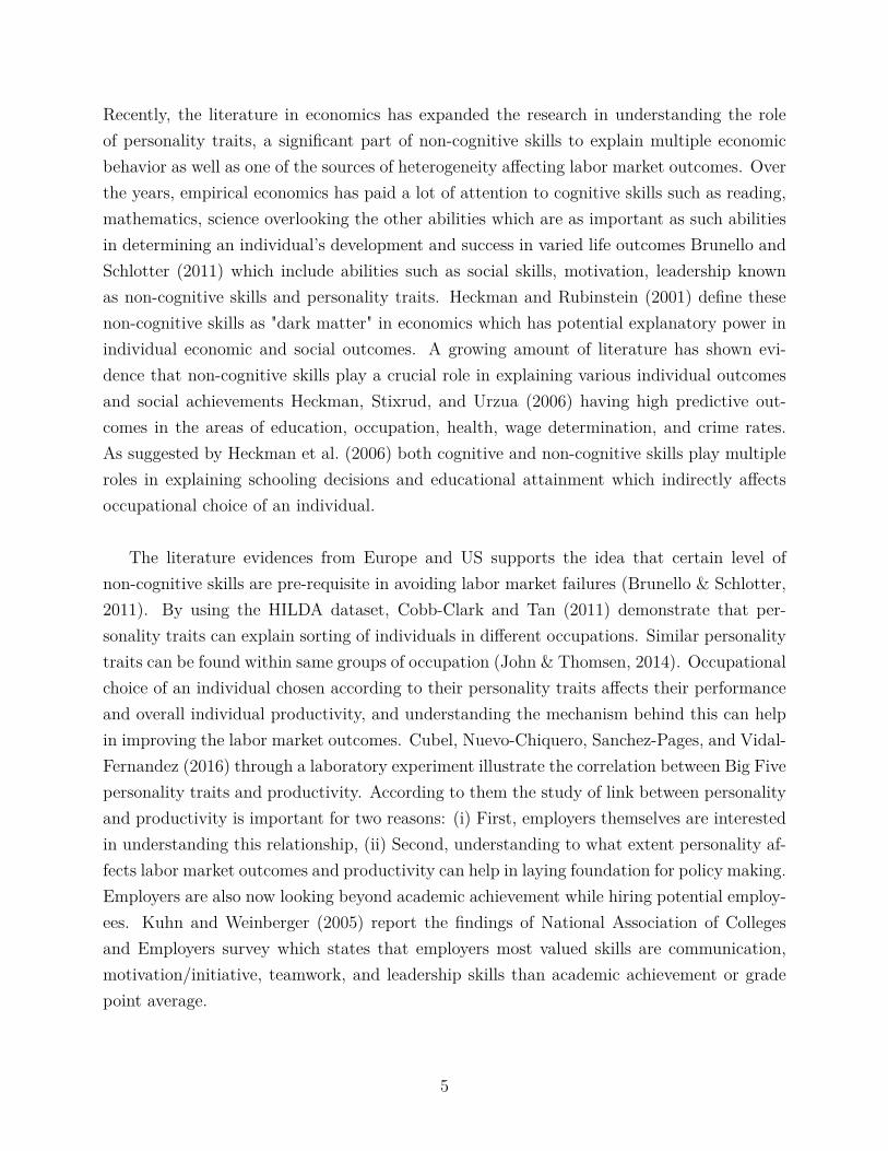
Recently, the literature in economics has expanded the research in understanding the roleof personality traits, a significant part of non-cognitive skills to explain multiple economicbehavior as well as one of the sources of heterogeneity affecting labor market outcomes. Overthe years, empirical economics has paid a lot of attention to cognitive skills such as reading,mathematics, science overlooking the other abilities which are as important as such abilitiesin determining an individual’s development and success in varied life outcomes Brunello andSchlotter (2011) which include abilities such as social skills, motivation, leadership knownas non-cognitive skills and personality traits. Heckman and Rubinstein (2001) define thesenon-cognitive skills as "dark matter" in economics which has potential explanatory power inindividual economic and social outcomes. A growing amount of literature has shown evi-dence that non-cognitive skills play a crucial role in explaining various individual outcomesand social achievements Heckman, Stixrud, and Urzua (2006) having high predictive out-comes in the areas of education, occupation, health, wage determination, and crime rates.As suggested by Heckman et al. (2006) both cognitive and non-cognitive skills play multipleroles in explaining schooling decisions and educational attainment which indirectly affectsoccupational choice of an individual.

The literature evidences from Europe and US supports the idea that certain level ofnon-cognitive skills are pre-requisite in avoiding labor market failures (Brunello & Schlotter,2011). By using the HILDA dataset, Cobb-Clark and Tan (2011) demonstrate that per-sonality traits can explain sorting of individuals in different occupations. Similar personalitytraits can be found within same groups of occupation (John & Thomsen, 2014). Occupationalchoice of an individual chosen according to their personality traits affects their performanceand overall individual productivity, and understanding the mechanism behind this can helpin improving the labor market outcomes. Cubel, Nuevo-Chiquero, Sanchez-Pages, and Vidal-Fernandez (2016) through a laboratory experiment illustrate the correlation between Big Fivepersonality traits and productivity. According to them the study of link between personalityand productivity is important for two reasons: (i) First, employers themselves are interestedin understanding this relationship, (ii) Second, understanding to what extent personality af-fects labor market outcomes and productivity can help in laying foundation for policy making.Employers are also now looking beyond academic achievement while hiring potential employ-ees. Kuhn and Weinberger (2005) report the findings of National Association of Collegesand Employers survey which states that employers most valued skills are communication,motivation/initiative, teamwork, and leadership skills than academic achievement or gradepoint average.

5

A widely accepted taxonomy in the empirical economics literature to measure personalitytraits is the Big Five Model which includes the factors : agreeableness, conscientiousness,openness, extraversion and neuroticism. Agreeableness is defined as the tendency to act in anunselfish, cooperative manner. Conscientiousness is when an individual acts in an organised,responsible and hardworking manner. Openness is the tendency of an individual to be opento new culture, experience, and aesthetic. Extraversion associates with individuals who havea preference for human contacts, empathy, and assertiveness. Individual with extraversionprefer more outer world people and things rather than inner world of subjective things. Theyare sociable and have positive effect. Neuroticism refers to an individual has emotional in-stability (Todd & Zhang, 2020). By using the Big Five Model as a measure of personalitytraits, John and Thomsen (2014) provide evidence that occupational sorting is influencedby non-cognitive skills and that there is an inter-dependency of personality, occupation andwages, underlying the importance of occupation specific evaluation of returns. Ham et al.(2009b) use the HILDA survey to study the effects on the probability of being in a whitecollar occupation and find that along with human capital, parental status and personalitytraits have significant effects on occupational outcomes, and that effect of conscientiousnessis larger. Ham, Junankar, and Wells (2009a) find that human capital has non-linear effectson occupational choice, and that parental status has minimal effect whereas the Big FiveModel has a significant, persistent effect over occupational outcomes. Using the HILDA sur-vey data, they find are that managers are less agreeable and more antagonistic; labourersare less conscientiousness; and sales people are more extraverted. Similar kind of evidence isalso found by Nieken and Störmer (2010) using the German Socio-Economic Panel(GSOEP)data set providing the evidence of individuals with different personality traits associated withdifferent occupations.

Apart from human capital and personality traits, another source of heterogeneity con-tributing to varied occupations in labor market is the role of parents. The influence of parentson occupational choice can be considered via two channels : firstly, the effect of status ofindividual’s parents within the society which is referred as "dynasty hysteresis", and sec-ondly through intergenerational transmission skills. In the first way of influence, dynastyhysteresis can be defined as an individual’s parents achievements, abilities, and skills caninfluence an individual’s occupational choice and due to such a transfer mechanism, parentsand offspring’s are often found in the same occupation. Existing literatures provide evidencesof dynasty hysteresis which can be caused due to different reasons, such as human capitaltransfer, religion and its associated characteristics, social groups, and preferences (Ham etal., 2009a). Regardless of different causes, dynasty is an important phenomenon which has a

6

huge potential to influence an individual’s decisions regarding occupational choice. Constantand Zimmermann (2003) examine the effects of parental social status and find that it hassignificant effect on an individual’s occupational choice. They find that family backgroundaffects occupational choice through genetic endowment, social connections, wealth, and in-directly through education. Though, evidences of causes and presence of dynasty hysteresishas been documented in literatures, the mechanism is still under debate.

In the second way of influence an individual’s occupational choice is can be seen throughintergenerational transmission of skills from parents which can be both cognitive and non-cognitive skills. There are two main channels of transmission of cognitive and non-cognitiveskills between generations posited. It can be transmitted through inheritance of genes(nature)and through productivity effect of parental skills (nurture) (Anger, 2012). Cognitive skillsare based on past learning and are more strongly transmitted when related to innate abilityhighlighting the importance of parental investments in children’s cognitive outcomes (Anger& Heineck, 2010). Cunha and Heckman (2008) find evidence that parental input affects theformation of both cognitive and non-cognitive and that parental inputs affect the forma-tion of cognitive skills more strongly at earlier ages. Chevalier et al. (2002) conclude thatoccupational choices of UK graduates are same as that of their father after 6-11 years ofgraduation and that their decision is mainly based on their father’s education and occupa-tion. An individual’s skill level changes with time from childhood into adulthood as a resultof education, work experience and training. de Coulon et al. (2011) conduct a research tostudy how strong is parent’s adult skill levels help in predicting their children’s cognitive andnon-cognitive skills and their results indicate that parent’s with high numeracy and literacyskills have children with higher cognitive and non-cognitive skills.

The literature review highlights that in the labor market occupational choice of an individ-ual to a great extent influence their productivity levels. It also highlights that occupationalchoice of a personal can be influenced through multiple factors such as cognitive skills, non-cognitive skills, occupation of parents among others. With this, the objective of the thesis isto understand the intergenerational transmission of both cognitive and non-cognitive skillsfrom parent to child and its role in influencing the occupational choice of the individual andamong these two skills which is more influential in impacting the occupational choice of anindividual?

The outline of rest of the thesis follows in this way: In section 2, LISREL methodologyis described in detail following which in section 2.3, an example is illustrated to elucidate

7

the methodology. In section 3, an overview of the model is described consisting of threeparts, namely, measurement model, structural model, and occupational choice model alongwith identification of factor loadings. Section 4 discusses the estimation techniques for themeasurement model and structural model. It also discusses the reliability of factors and var-ious measures of goodness-of-fit indices. Section 5 presents the data along with the differentsets of variables considered which is followed by results of the estimated model in section6. Finally, in section 7 conclusion along with discussion is presented with further scope ofresearch.

8

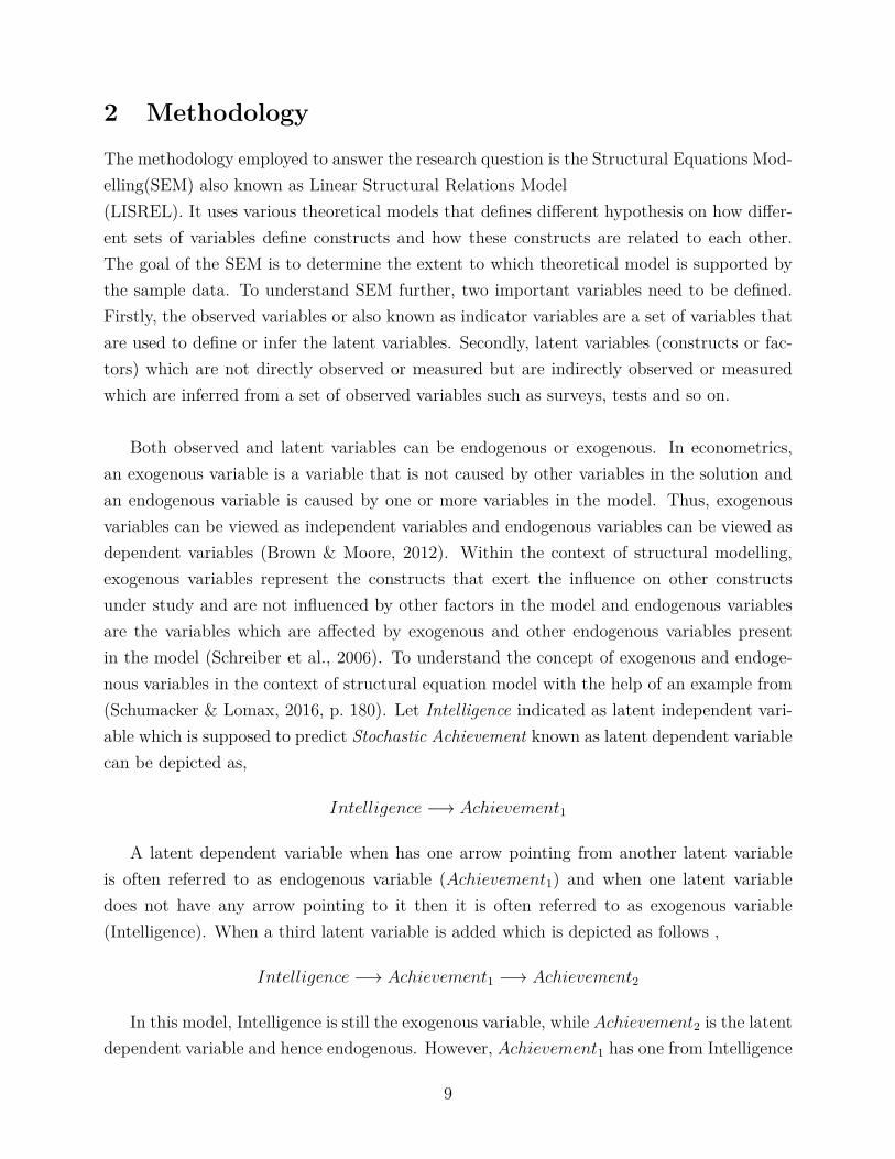
2 Methodology

The methodology employed to answer the research question is the Structural Equations Mod-elling(SEM) also known as Linear Structural Relations Model(LISREL). It uses various theoretical models that defines different hypothesis on how differ-ent sets of variables define constructs and how these constructs are related to each other.The goal of the SEM is to determine the extent to which theoretical model is supported bythe sample data. To understand SEM further, two important variables need to be defined.Firstly, the observed variables or also known as indicator variables are a set of variables thatare used to define or infer the latent variables. Secondly, latent variables (constructs or fac-tors) which are not directly observed or measured but are indirectly observed or measuredwhich are inferred from a set of observed variables such as surveys, tests and so on.

Both observed and latent variables can be endogenous or exogenous. In econometrics,an exogenous variable is a variable that is not caused by other variables in the solution andan endogenous variable is caused by one or more variables in the model. Thus, exogenousvariables can be viewed as independent variables and endogenous variables can be viewed asdependent variables (Brown & Moore, 2012). Within the context of structural modelling,exogenous variables represent the constructs that exert the influence on other constructsunder study and are not influenced by other factors in the model and endogenous variablesare the variables which are affected by exogenous and other endogenous variables presentin the model (Schreiber et al., 2006). To understand the concept of exogenous and endoge-nous variables in the context of structural equation model with the help of an example from(Schumacker & Lomax, 2016, p. 180). Let Intelligence indicated as latent independent vari-able which is supposed to predict Stochastic Achievement known as latent dependent variablecan be depicted as,

Intelligence −→ Achievement1

A latent dependent variable when has one arrow pointing from another latent variableis often referred to as endogenous variable (Achievement1) and when one latent variabledoes not have any arrow pointing to it then it is often referred to as exogenous variable(Intelligence). When a third latent variable is added which is depicted as follows ,

Intelligence −→ Achievement1 −→ Achievement2

In this model, Intelligence is still the exogenous variable, while Achievement2 is the latentdependent variable and hence endogenous. However, Achievement1 has one from Intelligence

9

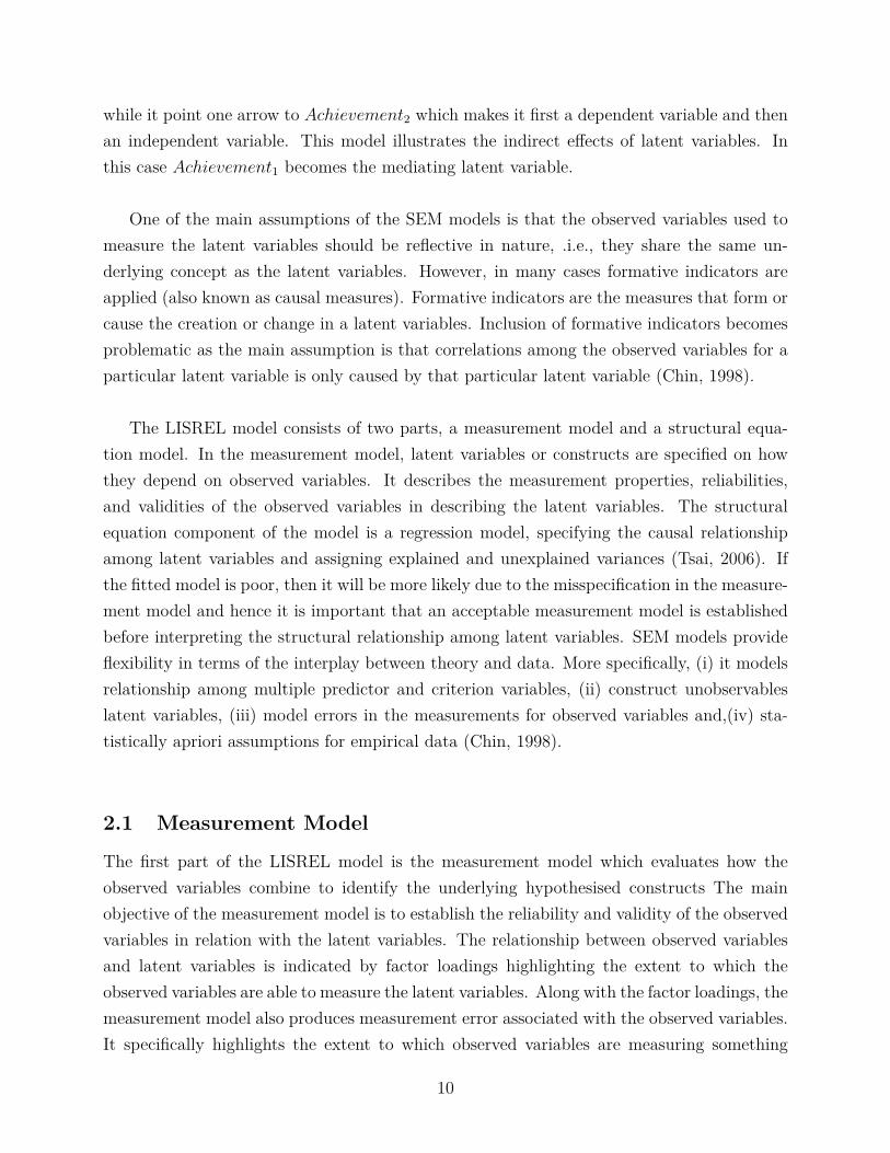
while it point one arrow to Achievement2 which makes it first a dependent variable and thenan independent variable. This model illustrates the indirect effects of latent variables. Inthis case Achievement1 becomes the mediating latent variable.

One of the main assumptions of the SEM models is that the observed variables used tomeasure the latent variables should be reflective in nature, .i.e., they share the same un-derlying concept as the latent variables. However, in many cases formative indicators areapplied (also known as causal measures). Formative indicators are the measures that form orcause the creation or change in a latent variables. Inclusion of formative indicators becomesproblematic as the main assumption is that correlations among the observed variables for aparticular latent variable is only caused by that particular latent variable (Chin, 1998).

The LISREL model consists of two parts, a measurement model and a structural equa-tion model. In the measurement model, latent variables or constructs are specified on howthey depend on observed variables. It describes the measurement properties, reliabilities,and validities of the observed variables in describing the latent variables. The structuralequation component of the model is a regression model, specifying the causal relationshipamong latent variables and assigning explained and unexplained variances (Tsai, 2006). Ifthe fitted model is poor, then it will be more likely due to the misspecification in the measure-ment model and hence it is important that an acceptable measurement model is establishedbefore interpreting the structural relationship among latent variables. SEM models provideflexibility in terms of the interplay between theory and data. More specifically, (i) it modelsrelationship among multiple predictor and criterion variables, (ii) construct unobservableslatent variables, (iii) model errors in the measurements for observed variables and,(iv) sta-tistically apriori assumptions for empirical data (Chin, 1998).

2.1 Measurement Model

The first part of the LISREL model is the measurement model which evaluates how theobserved variables combine to identify the underlying hypothesised constructs The mainobjective of the measurement model is to establish the reliability and validity of the observedvariables in relation with the latent variables. The relationship between observed variablesand latent variables is indicated by factor loadings highlighting the extent to which theobserved variables are able to measure the latent variables. Along with the factor loadings, themeasurement model also produces measurement error associated with the observed variables.It specifically highlights the extent to which observed variables are measuring something

10

other than the proposed latent variable (Shanmugam & Marsh, 2015). While generating themeasurement model defining the latent variables the following questions needs to addressed:To what extent are the observed variables actually measuring the latent variables? Whichof the observed variables are the best predictors of the latent variables? Are the observedvariables measuring something other than latent variables?

2.1.1 Confirmatory factor analysis

The measurement model uses confirmatory factor analysis (CFA) model to confirm that ahypothesised latent variable can be inferred from observed variables. In CFA, one can findout the extent to which the items used to measure a latent variable are related to one anotherbut also the latent variable can be determined by examining the loadings of the observedvariables. CFA is an effect indicator model. The use of CFA goes beyond rejecting or con-firming a factor model, where one can also revise, refine and retest the model using a welldefined set of criteria (Phakiti, 2018). It specifies the number of factor loadings to reflectthat only certain factors can influence certain factor indicators by fixing many or all crossloadings equal to zero. And by incorporating the prior knowledge in the form of restrictions,the definition of latent variables is more subjective and also leads to a parsimonious mod-els. However, fixing many or all cross loadings equal to zero may lead to a parsimoniousmodel than suitable to the data which then leads to multiple respecification Asparouhov andMuthén (2009). In the confirmatory factor model, the relationship between observed andlatent variables is explained. Each factor indicates gives the information to what extent anobserved variable is able to measure the latent variable. To avoid misspecification in themodel, one has to define latent variable accurately so that the measures defined are stronglycorrelated with each. If weakly correlated, then the constructs will be poorly defined andlead to model misspecification (Weston & Gore Jr, 2006).

In the CFA model, there are three types of parameters specified, namely, free, fixed, orconstrained. A free parameter is unknown which has to be estimated by minimizing thedifferences between the observed and predicted variance-covariance matrices. A fixed param-eter is pre-specified to a specific value mostly equalling to 1 or 0. A constrained parameteris unknown, however the parameter is not free to be any value, some restrictions are placedon the value it may assume. One of the most common constraints is the equality constraintsin which some of the parameters in CFA solutions is restricted to be equal in value (Brown& Moore, 2012).

CFA is confined to the analysis of variance-covariance structures and the analysis of the

11

covariance structures is based on the assumption that indicators are measured as deviationfrom the means (Brown & Moore, 2012). While conducting CFA, the researcher uses ahypothesised model to estimate a population covariance matrix which is then compared withthe observed covariance matrix. The main goal is to minimise the difference between theestimated and observed matrices(Schreiber et al., 2006).

2.2 Structural Model

The second part of the LISREL model is the structural model which is similar to the regressionmodel explaining the causal relationship between independent and dependent variables asspecified in the measurement model. The structural model explains how the latent variablesare related among each other. After specifying the hypothesised structural model, it can betested to determine the extent to which these priories are supported by the sample variance-covariance data. Each structural equation contains a prediction error which explains theportion of variance that is not explained by the latent variables (Schumacker & Lomax,2016, p. 187).

2.3 LISREL Illustrated Example

In this section two examples have been illustrated in figure 1 and 2 to explain the LISRELmodel combining the measurement and structural part of the model. The example in figure1 is a properly specified structural equation some parameters are fixed while some are freewhich needs to be estimated and figure 2 explains a simple form of a MIMIC model.

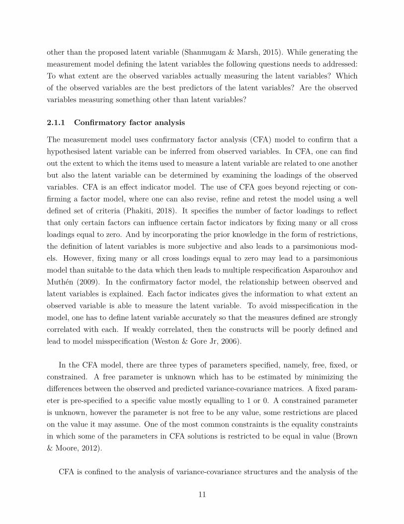
Figure 1: Example of a simple LISREL model from (Lei & Wu, 2007)

Figure 1 shows a model that predicts reading(READ) and mathematics(MATH) latentability variables from two observed scores of intelligence namely, verbal comprehension(VC)and perpetual organisation(PO). The latent variable READ is indicated by basic word read-ing(BW) and reading comprehension(RC) scores, while the latent variable MATH is indicated

12

by calculation(CL) and reasoning(RE) scores. The paths denoted by directional arrow fromVC and PO to READ and MATH, from READ to BW and RC, and from MATH to CLand RE along with curved arrows between VC and PO, and between residuals of READ andMATH are the free parameters to be estimated in the model as well as the residuals of theendogenous and exogenous variables. The remaining paths which are not shown will not beestimated and are fixed to zero. The scale of the latent variable can be standardised by fixingits variance to 1 or the latent variable can take the scale of one of its indicator variables byfixing the first factor loading of one indicator to 1. When the parameter value of a path isfixed to a constant, the parameter will not be estimated from the data.

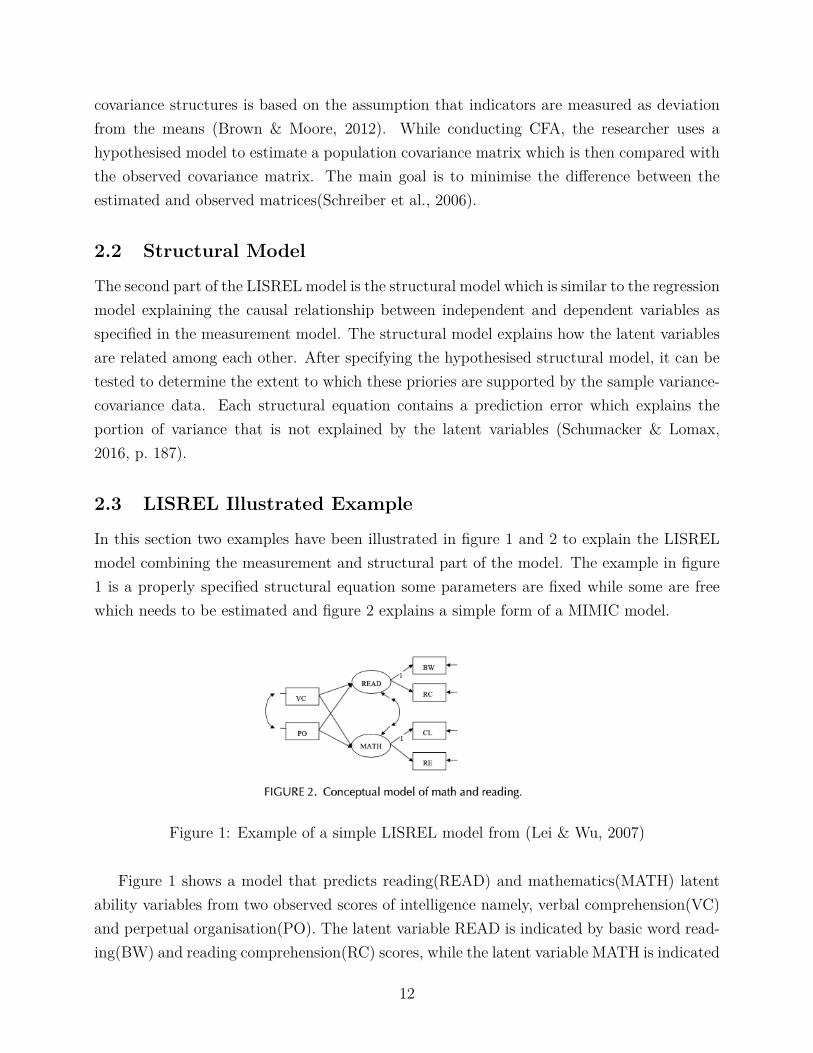
Figure 2: Example of a MIMIC model from (Schumacker & Lomax, 2016, p. 294)

MIMIC model is a special case of SEM models known as multiple indicators and multiplecauses model which involves using latent variables predicted by the observed variables. Figure2 is a representation of a simple MIMIC model in which latent variable social participationis defined by observed variables church attendance, memberships, and friends. Further thelatent variable social participation is predicted by observed variables income, occupation andeducation. In the above MIMIC model, social which is a latent variable has arrows pointingout to three observed variables(church, member,and friends) along with their respective mea-surement error for each. This part is the measurement part of the model. Now, the latentvariable social also has arrows pointed towards it from three observed predictor variableswhich are correlations among them. This is the structural part of the model which usesobserved variables to predict latent variables (Schumacker & Lomax, 2016).

13

3 Model

The model used to answer the research objective combines multiple indicator multiple cause(MIMIC) and LISREL model helping in the process of identification of restrictions of crossequations. MIMIC is a special case of the SEM models which permits the specification ofone or more latent variables with one or more observed variables as predictors of latent vari-ables (Schumacker & Lomax, 2016, p. 293). It incorporates additional variables which areassumed to influence the latent factors. The MIMIC model introduces the causes of latentfactors. As proposed by Jöreskog and Goldberger (1975) , in the MIMIC model, one observesmultiple indicators and multiple causes of a single latent variable. The observed variablesresult from the latent factors and the latent factors themselves are caused by other exogenousvariables. Thus, there is a measurement equation and a causal relationship (Krishnakumar& Nagar, 2008). The model comprises of three parts, the first part is the measurement modelusing confirmatory factor model, second part is the structural model which uses factor scoreregression and the third part is a factor score regression to understand the influence of inter-generational transmission of skills from parents and occupation of parents in the individual’schoice of occupation.

3.1 Part I: Measurement Model

The first part of the model is a measurement model for which a confirmatory factor model isfitted to understand the extent to which the underlying indicators measure the latent variable.The CFA model was fitted for individual and mother’s cognitive, non-cognitive skills alongwith parental investments. The measurement model to account for the individual’s cognitiveand non-cognitive skills is given by,

Xki,t−1 = Λk

0i,t−1 + Λk1i,t−1θ

kt−1 + εk1i,t−1 (1)

Xki,t = Λk

0i,t + Λk2i,tθ

kt + εk2i,t (2)

with k ∈ (C,N, I, PC, PI). X represents the observed measures of latent variables wherei = 1, ...mk denoting different indicators of specific latent variable. Here C is the cognitiveskills of the individual, N is the non-cognitive skills of the individual, PC is the mother’snon-cognitive skills, PN is the mother’s non-cognitive skills and I is the parental investment.θ is the factor for the latent variable and Λi,t is the respective factor loading.

14

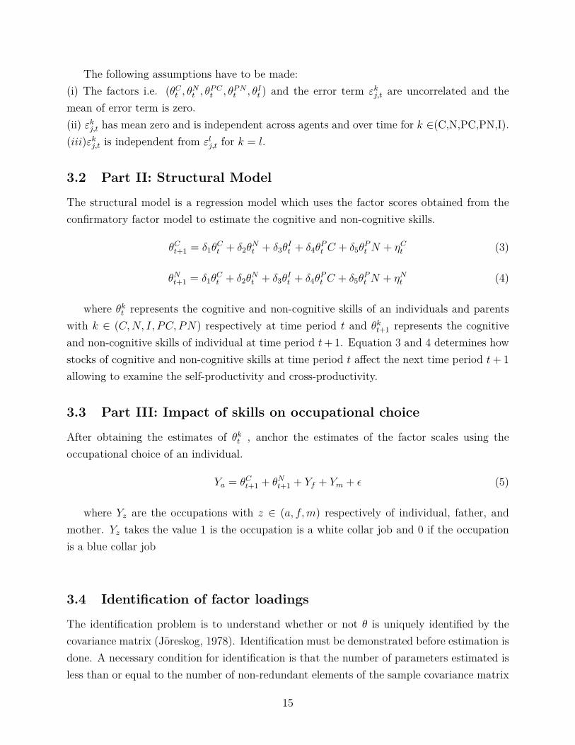
The following assumptions have to be made:(i) The factors i.e. (θCt , θ

Nt , θ

PCt , θPN

t , θIt ) and the error term εkj,t are uncorrelated and themean of error term is zero.(ii) εkj,t has mean zero and is independent across agents and over time for k ∈(C,N,PC,PN,I).(iii)εkj,t is independent from εlj,t for k = l.

3.2 Part II: Structural Model

The structural model is a regression model which uses the factor scores obtained from theconfirmatory factor model to estimate the cognitive and non-cognitive skills.

θCt+1 = δ1θCt + δ2θ

Nt + δ3θ

It + δ4θ

Pt C + δ5θ

Pt N + ηCt (3)

θNt+1 = δ1θCt + δ2θ

Nt + δ3θ

It + δ4θ

Pt C + δ5θ

Pt N + ηNt (4)

where θkt represents the cognitive and non-cognitive skills of an individuals and parentswith k ∈ (C,N, I, PC, PN) respectively at time period t and θkt+1 represents the cognitiveand non-cognitive skills of individual at time period t+1. Equation 3 and 4 determines howstocks of cognitive and non-cognitive skills at time period t affect the next time period t+ 1

allowing to examine the self-productivity and cross-productivity.

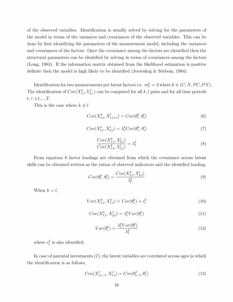
3.3 Part III: Impact of skills on occupational choice

After obtaining the estimates of θkt , anchor the estimates of the factor scales using theoccupational choice of an individual.

Ya = θCt+1 + θNt+1 + Yf + Ym + ϵ (5)

where Yz are the occupations with z ∈ (a, f,m) respectively of individual, father, andmother. Yz takes the value 1 is the occupation is a white collar job and 0 if the occupationis a blue collar job

3.4 Identification of factor loadings

The identification problem is to understand whether or not θ is uniquely identified by thecovariance matrix (Jöreskog, 1978). Identification must be demonstrated before estimation isdone. A necessary condition for identification is that the number of parameters estimated isless than or equal to the number of non-redundant elements of the sample covariance matrix

15

of the observed variables. Identification is usually solved by solving for the parameters ofthe model in terms of the variances and covariances of the observed variables. This can bedone by first identifying the parameters of the measurement model, including the variancesand covariances of the factors. Once the covariance among the factors are identified then thestructural parameters can be identified by solving in terms of covariances among the factors(Long, 1983). If the information matrix obtained from the likelihood estimation is positivedefinite then the model is high likely to be identified (Joereskog & Sörbom, 1984).

Identification for two measurements per latent factors i.e. mkt = 2 where k ∈ (C,N, PC, PN).

The identification of Cov(Xk1,t, Y

l2,τ ) can be computed for all k, l pairs and for all time periods

t, τ ∈1,...,T.

This is the case where k = l

Cov(Xk1,t, X

l1,t+1) = Cov(θkt , θ

lt) (6)

Cov(Xk1,t, X

l2,t) = λk

tCov(θkt , θlt) (7)

Cov(Xk1,t, X

l2,t)

Cov(Xk1,t, X

l1,t)

= λkt (8)

From equation 8 factor loadings are obtained from which the covariance across latentskills can be obtained written as the ration of observed indicators and the identified loading,

Cov(θkt , θlt) =

Cov(Xk1,t, X

l2,t)

λkt

(9)

When k = l,

V ar(Xk1,t, X

k1,t) = V ar(θkt ) + ϵkt (10)

Cov(Xk1,t, X

l2,t) = λk

t V ar(θkt ) (11)

V ar(θkt ) =λkt V ar(θkt )

λkt

(12)

where ϵkt is also identified.

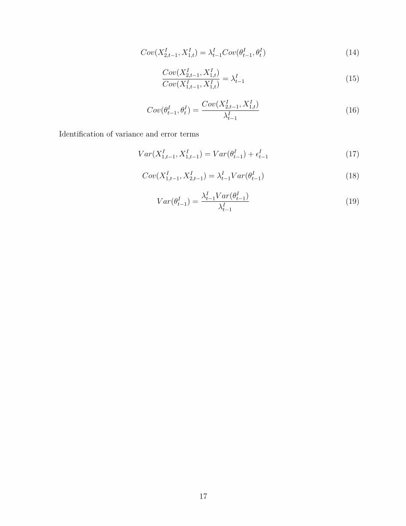
In case of parental investments (I), the latent variables are correlated across ages in whichthe identification is as follows,

Cov(XI1,t−1, X

I1,t) = Cov(θIt−1, θ

It ) (13)

16

Cov(XI2,t−1, X

I1,t) = λI

t−1Cov(θIt−1, θIt ) (14)

Cov(XI2,t−1, X

I1,t)

Cov(XI1,t−1, X

I1,t)

= λIt−1 (15)

Cov(θIt−1, θIt ) =

Cov(XI2,t−1, X

I1,t)

λIt−1

(16)

Identification of variance and error terms

V ar(XI1,t−1, X

I1,t−1) = V ar(θIt−1) + ϵIt−1 (17)

Cov(XI1,t−1, X

I2,t−1) = λI

t−1V ar(θIt−1) (18)

V ar(θIt−1) =λIt−1V ar(θIt−1)

λIt−1

(19)

17

4 Estimation

4.1 Estimation of measurement models

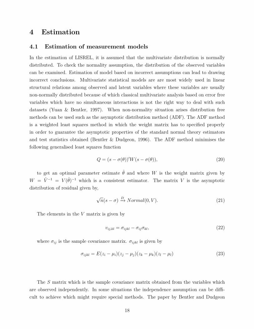
In the estimation of LISREL, it is assumed that the multivariate distribution is normallydistributed. To check the normality assumption, the distribution of the observed variablescan be examined. Estimation of model based on incorrect assumptions can lead to drawingincorrect conclusions. Multivariate statistical models are are most widely used in linearstructural relations among observed and latent variables where these variables are usuallynon-normally distributed because of which classical multivariate analysis based on error freevariables which have no simultaneous interactions is not the right way to deal with suchdatasets (Yuan & Bentler, 1997). When non-normality situation arises distribution freemethods can be used such as the asymptotic distribution method (ADF). The ADF methodis a weighted least squares method in which the weight matrix has to specified properlyin order to guarantee the asymptotic properties of the standard normal theory estimatorsand test statistics obtained (Bentler & Dudgeon, 1996). The ADF method minimises thefollowing generalised least squares function

Q = (s− σ(θ))′W (s− σ(θ)), (20)

to get an optimal parameter estimate θ and where W is the weight matrix given byW = V −1 = V (θ)−1 which is a consistent estimator. The matrix V is the asymptoticdistribution of residual given by,

√n(s− σ)

D−→ Normal(0, V ). (21)

The elements in the V matrix is given by

vij,kl = σijkl − σijσkl, (22)

where σij is the sample covariance matrix. σijkl is given by

σijkl = E(zi − µi)(zj − µj)(zk − µk)(zl − µl) (23)

The S matrix which is the sample covariance matrix obtained from the variables whichare observed independently. In some situations the independence assumption can be diffi-cult to achieve which might require special methods. The paper by Bentler and Dudgeon

18

(1996) the argument is that the values of the parameters can be estimated from the samplecovariance matrix S and can be tested for the fit of the model in the population covariancematrix Σ(θ) by minimizing some scalar function F = F [S,Σ(θ)]. The scalar function F

indicates the discrepancy between S and Σ(θ). The discrepancy function F has the followingproperties: (i) the value of F will be greater than or equal to zero ,(ii) F will only be equalto zero if S = Σ(θ), and (iii) F must be twice differentiable with respect to both S and Σ(θ).Some of the examples of the discrepancy function are ML and GLS. In case of a distributionfree deployed, the results obtained will always be optimal as the discrepancy function wouldalways be correctly specified which was introduced by Browne (1982) and minimum distancemethod by (Chamberlain, 1982).

A study by Benson and Fleishman (1994) compared the robustness of both ML andADF methods using Monte Carlo simulation to investigate the combined effects of samplesize, magnitude of correlation among observed indicators, number of indicators, magnitudeof skewness and kurtosis. Their results indicated a little bias in the factor loadings in bothML and ADF estimation under all conditions studied. The bias was seen more in ADFthan ML as the number of indicators increased. Increase in skewness and kurtosis showedunderestimation of standard errors with ML standard errors being more biased than ADFunder non-normality conditions, and ML chi-square was also inflated. A comparison studybetween pseudo-likelihood (p-ML) and ADF by Molenaar and Nesselroade (1998) shows thatboth the methods tend to give consistent parameter estimates, but the standard errors andchi-square statistics appears to be more consistent in the ADF method.

The model fit is of the CFA is found to be inadequate, can be improved by using themodification indices in which certain parameters are added or deleted. The value given bythe modification indices is the minimum amount that the chi-square value is expected todecrease if the corresponding parameters is fixed. A parameter is freed to improve the fit ofthe model and this process continues until an adequate fit is obtained.

4.2 Estimation of structural regression model

The classic approach of modelling structural equation models is by using one-step approachwhere both measurement and structural part are estimated simultaneously. However, simul-taneous estimation of both parts can suffer from interpretational confounding which getsreflected in the parameter coefficients of the estimates. Interpretational confounding "occursas the assignment of empirical meaning of unobserved variable which is other than meaningof assigned to it by an individual which is other than meaning assigned to it by an indi-

19

vidual a priori to estimating unknown parameters" (Burt, 1976, p. 4). It can be explainedas the changes in the coefficients when alternate structural models are estimated. But theinterpretational confounding can be minimized by prior separate estimation of the measure-ment model to put no constraints on the structural parameters. A two-step approach focuseson the tradeoff between goodness of fit and strength of the causal inference. And sepa-rate assessment of measurement and structural model preclude having good fit of one modelcompensate for poor fit for other (Anderson & Gerbing, 1988). According to Bollen (1996)misspecification errors in one part of the equation can spillover to other parts of the equationwhen simultaneously estimated. The first part consists of measurement equation model inthe two-step procedure factor analysis is performed using CFA through which factor scoresare calculated, where the factor scores are estimated for the true latent variables. The factorscores are usually predicted using either regression predictor or Bartlett predictor. In thesecond part, the factor scores are used in linear regression considering them to be true latentvariable scores. However, the use of factor scores directly leads to a bias in the estimatesobtained. The bias is due to the covariance matrix of the factor scores and the true latentvariables being different.

4.2.1 Bias Corrected factor score regression

According to Skrondal and Laake (2001), the performance of conventional factor score re-gression is quite bad. To avoid bias, their methodology of revised factor score comprisedof using regression factor scores for the explanatory latent variables and for the responselatent variables Bartlett scores were used to provide consistent estimators for all parameters.This method however fails when there are correlations between independent variables. Onthe other hand, Croon (2002) corrects bias. According to him, there is a difference betweenvariances and covariances of the factor scores and the latent variables and hence uses anestimation of variances and covariances of true latent variable instead of the factor scores toestimate the regression parameters. This method can be used any estimator and predictor.Devlieger and Rosseel (2017) summarise the method of Croon,

1. Perform factor analysis for all the latent variables separately and obtain the respectivefactor scores.

2. Calculate the variance-covariance matrix of factor scores.

3. Estimate the true variance and covariances for all the elements in this variance-covariancematrix.

20

4. Perform regression using the estimated variance-covariance matrix as the input for thecovariance in the model.

The bias corrected formula proposed by Croon for the variance and covariance is givenas follows,

var(ξ) =var(Fξ)− AξΘδA

′ξ

AξΛxΛ′xA

′ξ

, (24)

cov(ξ, η) =cov(Fξ, Fη)

AξΛxΛ′yA

′η

. (25)

where, Λx and Λy are the factor loadings, Aξ and Aη are the factor score matrices, andΘδ is the variance-covariance matrix of the unique factor scores of δ. Equation 25 show thatcorrected covariance can be obtained by dividing the covariance among factor scores andproducts of the factor scores and loading matrices. One of the key insights of equation 25is that matrix multiplication in the denominator gives the product of construct reliabilities,i.e., each matrix multiplication of the individual factor score and loading matrices producesempirical estimates of construct reliabilities on the basis of measurement models. To correctthe variances, we can set each term of the latent variable to one on the diagonal of thecovariance matrix.

4.3 Reliability of factors

The reliability part in the measurement model is the part containing no random error. Interms of SEM models, the reliability of an indicator is defines as the variance of the indicatorthat is not accounted by the measurement error, represented by squared multiple correlationcoefficient ranging from 0 to 1 (Raines-Eudy, 2000). Measurement is an important aspectin the structural equation modelling and presence of measurement error can produce biasedestimates among the constructs. The most commonly used reliability measure is the alpha,where the the measurement model is assumed to be tau equivalence which i.e., true scoreequivalent where the factor loadings are equal. This has found to be quite misleading due toit being restricted and hence unrealistic. An alternative is the coefficient omega by McDonald(1999) in which the reliability estimates are calculated from the parameter estimates of thefactor models which are specified to represent associations between the items and constructs.Here the measurement model is assumed to be congeneric model in which the items areaffected by a single factor but with varying degrees termed as one factor confirmatory factormodel. As the model expands, consisting of more than one factor, it can be termed as multiple

21

regression equation with each xj regressed on multiple factors (Viladrich, Angulo-Brunet, &Doval, 2017). The coefficient omega is given as follows,

ωu =(∑J

j=1 λj)2

σX2 , (26)

ωh =(∑J

j=1 λjg)2

σX2 (27)

The factor loading is the strength of the association between the items and factors, mean-ing the extent to which a set of items reliably measures the factors and hence the reliabilitycan be estimated from the parameter estimates fitted to the item scores. Equation 26 isreliability of the one factor model where the numerator represents amount of total varianceexplained by the common factor as a function of estimated factor loadings, while the de-nominator represents the estimated variance of the observed total score. On the other hand,equation 27 represents the reliability of a two factor model where λjg is the factor loading ofxj on a general factor g. The total score variance represented by σX

2 can be calculated fromthe model implied variance of X.

Raykov (1998) proposed a method to obtain standard errors and confidence intervals in astructural equation modelling framework for estimating the reliability of congeneric measuresusing bootstrap method. In this approach he takes repeated samples from a given sampleto estimate reliability. The advantages of this method is that firstly, it is applicable to anyset of measures assessing a common latent variable which basically means that it should bea one factor confirmatory model. Secondly, it is applicable to non-normal observed variabledistributions. Thirdly, this method can be applied to weighted and unweighted scales.

4.4 Goodness-of-fit indices

Goodness-of-fit and its assessment is a key in the measurement model so as to one can under-stand how well the model fit is. There are various ways to assess the model fit of the modelwhich determines to which extent the observed (S) and model implied (Σ) variance-covariancematrix differs. The most commonly used measures of model fit chi-square (χ2), goodness-of-fit index(GFI), adjusted goodness-of-fit index(AGFI) and root-mean-square residual in-dex(RMR). A significant χ2 value indicates that the observed and implied covariance ma-trices differ. Usually, one is interested in obtaining a non-significant χ2 value so that thedifference between observed and implied covariance matrix. However, the χ2 value is verysensitive to sample size and when the observed variables do not follow multivariate normality

22

because of which it can lead to erroneous conclusions. Given the sensitivity of χ2 to sam-ple size, other measures of goodness-of-fit model are proposed which are some function ofchi-square and degrees of freedom. GFI is based on the ratio of sum of squared differencesbetween the observed and model implied covariance matrix to observed variance. The GFImeasures the amount of variance and covariance in S that is predicted by the Σ. To assesshow well the given model approximates the true model, Root Mean Square Error of Approx-imation(RMSEA) was introduced. If the approximation is good, then RMSEA should besmall where an acceptable value should be below 0.05. Another measure is the Root MeanSquare Residual (RMR) which is square root of the mean-squared differences between thematrix elements in S and Σ. An acceptable level of RMR is usually 0.05 and most oftenstandardised RMR are reported.

Several studies such as (Anderson and Gerbing (1984);Bearden et al. (1982)) suggeststhat parameter estimates are not affected by sample size or model characteristics, but thegoodness of fit indices have been affected, especially the chi square statistic, and GFI, RMR.Assumptions of chi-square tests violated by excessive kurtosis, moderate sample sizes, un-known statistical distributions, confidence intervals, little knowledge about the distributionand behaviour of fit indices for misspecified models are some of the reasons. The underlyingdistribution of test statistic is unknown in many instances and is often mathematically in-tractable. Bootstrapping is a general procedure for determining the sampling distribution ofa parameter estimate whose theoretical sampling distribution is unknown. Previous studieshave found that goodness of fit indices such as chi square statistics, root mean square errorare affected by model characteristics and as well sample size.

Bootstrap technique can be used to evaluate the goodness of fit indices of a confirma-tory factor model. A bias may be introduced if the bootstrapping sampling distribution isnon-normal and in such cases confidence interval estimated by percentile method i.e., biascorrected percentile method can be introduced (Bone et al., 1989). The general bootstrappingmethod can be described where there is a random sample X1, X2, ..., XN of size N with eachXi being drawn independently from the same population having a cumulative distributionG with parameter θ. We want to know the sampling distribution of the estimator θ. For thegiven random variables, there is a sample x1, x2, ..., xN . The bootstrap method samples fromthe population distribution defined by GN to estimate the sampling distribution of θ. Webootstrap sample, X∗

1 , X∗2 , ..., X

∗N by taking N draws with replacement from x1, x2, ..., xN .

The bootstrap estimate θ∗ is computed using the bootstrap sample. Repeating the processB times gives θ∗(1), θ∗(2), ..., θ∗(B). With these bootstrap replicates, mean and variance of

23

the θ can be obtained (Bollen & Stine, 1992). The general bootstrapping procedure worksin many cases, it can however fail as well.

The naive bootstrapping (completely non-parametric resampling from the original dis-tribution) is inaccurate as the distribution of the bootstrapped model test statistics followsa noncentral chi-square distribution instead of central chi-square distribution. (Bollen &Stine, 1992) formulated a transformation on the original data to adjust for this inaccuracywhich forces the resampling space to satisfy the null hypothesis (i.e., making the model-implied covariance matrix the true underlying covariance matrix in the population). Thetransformation is given by

Z = Y S−1/2Σ−1/2, (28)

where Y is the original data matrix from the parent sample. Analytically TML valuesfrom bootstrap samples drawn from transformed data matrix Z have an expectation equalto the model df . They also proposed a method to adjust for the p-value associated withTML. The bootstrap adjusted p-value is calculated as the proportion of bootstrap model teststatistics that exceed the value of TML obtained from the original parent sample.

24

5 Data

There are two different datasets used for this analysis, one for the parents and the secondfor the individual. Due to the limited availability of data, the dataset obtained is for theindividual with their respective mothers. For the mother, National Longitudinal Survey ofYouth 1979 (NLSY79) from where their cognitive skills, non-cognitive skills and occupationsvariables have been collected. While for the individual NLSY79 Child and Young Adultcohort(NLCY79) is used to obtain their cognitive skills, non-cognitive skills and occupationskeeping only those observations which match with mother’s ID. The NLSY79 is a longitudi-nal survey of men and women born during 1957-1964 in the United States when the surveybegan. Data collected in this survey provides information about the participants choices re-garding schooling, decisions regarding education and training, labor market, family life andexpectations about their retirement. NLCY79 is the longitudinal project which follows thebiological mothers from the NLSY79. The survey starts in 1986 where the mothers wereinterviewed every two years. The assessment include home environment, PIAT math andreading , Peabody Picture Vocabulary Test, the Digit Span scale of the Wechsler along withdetailed health information. Then starting in 1994, children aged 15 and older were inter-viewed based on the modified questionnaire of NLSY79 designing it according to the currentgeneration. Both these datasets were chosen due to its richness in the availability of vari-ables and its range covering wide topics. For the purpose of this analysis individuals bornto NLSY79 mothers after 1985 was only used which was 5722 observations, but for actualestimation only 3754 observations was only available due to the presence of missing values.

Mother’s cognitive ability is measured by the SAT and ACT scores in both mathemat-ics and verbal. Both these test scores were chosen to capture the mother’s cognitive abilitythrough their performance in standardised tests. Individual’s cognitive skills are measured byPeabody Individual Achievement Test(PIAT) for mathematics, reading comprehension andreading recognition. PIAT is a wide range measuring academic achievement for children agedfive and older, and the test if of high reliability and validity for the assessment of academicachievement. PIAT Math measures the child’s attainment in mathematics taught in main-stream education. PIAT Reading Recognition measures word recognition and pronunciationability while PIAT Reading Comprehension measures the child’s ability to derive meaningsfrom sentences. The items used to measure parental investments is the relationship of the in-dividual with biological parents, time parents spend with the individual on various occasions.

To measure the non-cognitive ability of mother, Rotter Locus of Control and Big Five

25

personality traits are used. Rotter Locus of Control measures the extent to which believethey have control over their lives either through self-motivation and self-determination de-fined as internal control as opposed to external control that conducts their life such as fate,luck. The higher the score, the individual will be more external. The Big Five personalitytraits measures the Big Five personality trait. For the individual,to measure non-cognitiveskills along with an additional measure Pearlin Mastery Scale and Big Five personality traits.Pearlin Mastery Scale refers to the measure of self-concept and references to the extent towhich individuals perceive themselves in control of forces that significantly impact their lives.At t, the individual’s age is 19 years in which an individual is assumed to make their educa-tional choices while at t + 1 individual’s age is 23 where the individual will be entering thejob market. For simplicity, parental investment and mother’s skills are taken to be constantfor both t and t+ 1

The Big Five personality trait consists of the following traits Openness, Conscientious-ness, Extraversion, Agreeableness, and Neuroticism which the respondent rates on a scaleof 1(Strongly Disagree) to 7 (Strongly Agree). The following are the indicators of each per-sonality trait are give by: Extraverted, enthusiastic (E); Dependable, self-disciplined (C);Anxious, easily upset (N); Open to new experiences, complex (O); Sympathetic, warm (A);Calm, emotionally stable (N, reversed). The indicators for the Rotter Locus of Control aregiven as follows: Degree of control one has over own life, importance of planning, importanceof luck, degree of influence one has over own life. While the indicators of the Pearlin Masteryscale is given as follows: No way I can solve the problems I have, I sometimes feel that Iam being pushed around, I have little control over what happens to me, I can do just aboutanything that happens in my life, I often feel helpless in dealing problems in my life, Whathappens to me in future mostly depends on me, Little I can do to change things in my life.

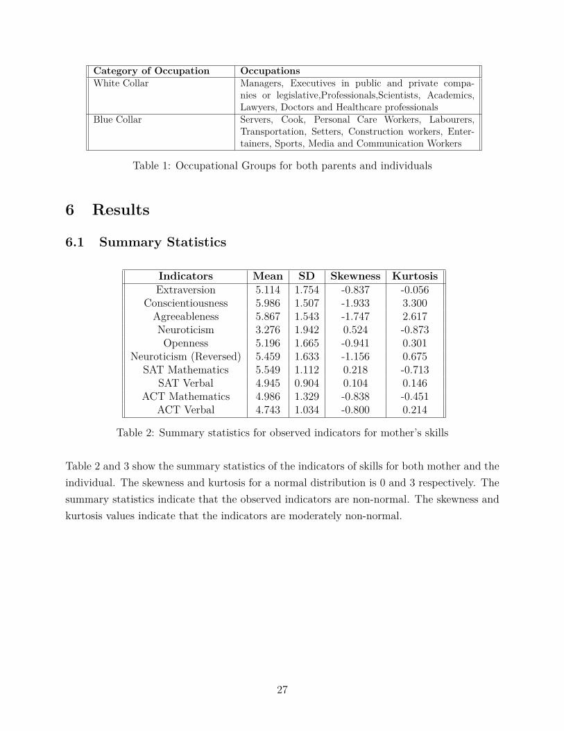
Table 1 contains the classification of occupation into white collar and blue collar jobfor the individual, mother and father. The occupations that come under white collar jobsconsists of office-related, non-manual jobs, while blue collar jobs are more of manual andindustrial occupations.

26

Category of Occupation OccupationsWhite Collar Managers, Executives in public and private compa-

nies or legislative,Professionals,Scientists, Academics,Lawyers, Doctors and Healthcare professionals

Blue Collar Servers, Cook, Personal Care Workers, Labourers,Transportation, Setters, Construction workers, Enter-tainers, Sports, Media and Communication Workers

Table 1: Occupational Groups for both parents and individuals

6 Results

6.1 Summary Statistics

Indicators Mean SD Skewness KurtosisExtraversion 5.114 1.754 -0.837 -0.056

Conscientiousness 5.986 1.507 -1.933 3.300Agreeableness 5.867 1.543 -1.747 2.617Neuroticism 3.276 1.942 0.524 -0.873Openness 5.196 1.665 -0.941 0.301

Neuroticism (Reversed) 5.459 1.633 -1.156 0.675SAT Mathematics 5.549 1.112 0.218 -0.713

SAT Verbal 4.945 0.904 0.104 0.146ACT Mathematics 4.986 1.329 -0.838 -0.451

ACT Verbal 4.743 1.034 -0.800 0.214

Table 2: Summary statistics for observed indicators for mother’s skills

Table 2 and 3 show the summary statistics of the indicators of skills for both mother and theindividual. The skewness and kurtosis for a normal distribution is 0 and 3 respectively. Thesummary statistics indicate that the observed indicators are non-normal. The skewness andkurtosis values indicate that the indicators are moderately non-normal.

27

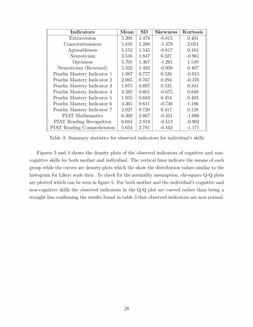
Indicators Mean SD Skewness KurtosisExtraversion 5.208 1.478 -0.815 0.401

Conscientiousness 5.810 1.288 -1.378 2.054Agreeableness 5.152 1.545 -0.817 0.164Neuroticism 3.516 1.847 0.327 -0.961Openness 5.705 1.367 -1.261 1.549

Neuroticism (Reversed) 5.322 1.492 -0.939 0.467Pearlin Mastery Indicator 1 1.987 0.777 0.526 -0.015Pearlin Mastery Indicator 2 2.065 0.767 0.294 -0.376Pearlin Mastery Indicator 3 1.875 0.697 0.535 0.344Pearlin Mastery Indicator 4 3.385 0.601 -0.675 0.848Pearlin Mastery Indicator 5 1.955 0.683 0.454 0.403Pearlin Mastery Indicator 6 3.365 0.611 -0.736 1.186Pearlin Mastery Indicator 7 2.027 0.720 0.417 0.128

PIAT Mathematics 6.369 2.867 -0.351 -1.086PIAT Reading Recognition 6.684 2.819 -0.513 -0.902

PIAT Reading Comprehension 5.654 2.781 -0.102 -1.171

Table 3: Summary statistics for observed indicators for individual’s skills

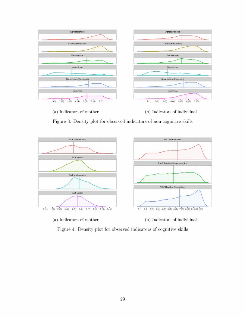
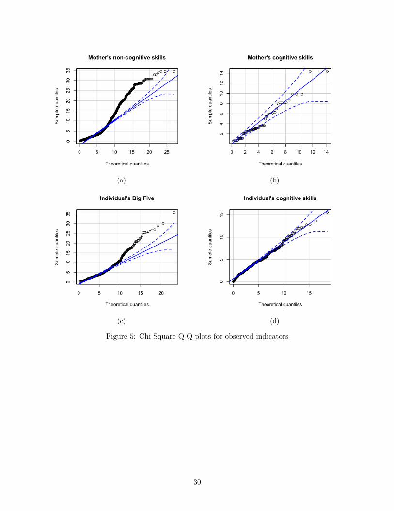
Figures 3 and 4 shows the density plots of the observed indicators of cognitive and non-cognitive skills for both mother and individual. The vertical lines indicate the means of eachgroup while the curves are density plots which the show the distribution values similar to thehistogram for Likert scale data. To check for the normality assumption, chi-square Q-Q plotsare plotted which can be seen in figure 5. For both mother and the individual’s cognitive andnon-cognitive skills the observed indicators in the Q-Q plot are curved rather than being astraight line confirming the results found in table 3 that observed indicators are non-normal.

28

(a) Indicators of mother (b) Indicators of individual

Figure 3: Density plot for observed indicators of non-cognitive skills

(a) Indicators of mother (b) Indicators of individual

Figure 4: Density plot for observed indicators of cognitive skills

29

(a) (b)

(c) (d)

Figure 5: Chi-Square Q-Q plots for observed indicators

30

6.2 Part I: Measurement Model

Latent Factor Indicator Factor LoadingsNon-Cognitive Skills (θPN

t )

Big Five(θPNb

t )

Extraversion 0.343(-)Agreeableness 0.610(0.137)

Conscientiousness 0.64(0.136)Neuroticism -0.203(0.099)Openness 0.530(0.113)

Neuroticism (Reversed) 0.603(0.131)

Rotter Scale(θPNr

t )

Rotter Locus of Control Indicator 1 0.223(0.045)Rotter Locus of Control Indicator 2 0.467(-)Rotter Locus of Control Indicator 3 0.266(0.058)Rotter Locus of Control Indicator 4 0.452(0.072)Rotter Locus of Control Indicator 5 0.262(0.035)Rotter Locus of Control Indicator 6 0.561(0.095)Rotter Locus of Control Indicator 7 -0.065(0.053)Rotter Locus of Control Indicator 8 0.316(0.071)

Neuroticism 0.163(0.240)Cognitive Skills (θPC

t )

Test Scores

SAT Mathematics 0.816(-)SAT Verbal 0.787(0.076)

ACT Mathematics 0.984(0.166)ACT Verbal 0.900(0.124)

Highest Grade of Mother 0.446(0.134)

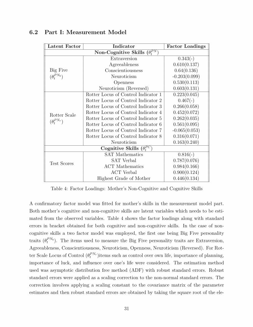
Table 4: Factor Loadings: Mother’s Non-Cognitive and Cognitive Skills

A confirmatory factor model was fitted for mother’s skills in the measurement model part.Both mother’s cognitive and non-cognitive skills are latent variables which needs to be esti-mated from the observed variables. Table 4 shows the factor loadings along with standarderrors in bracket obtained for both cognitive and non-cognitive skills. In the case of non-cognitive skills a two factor model was employed, the first one being Big Five personalitytraits (θPNb

t ). The items used to measure the Big Five personality traits are Extraversion,Agreeableness, Conscientiousness, Neuroticism, Openness, Neuroticism (Reversed). For Rot-ter Scale Locus of Control (θPNr

t )items such as control over own life, importance of planning,importance of luck, and influence over one’s life were considered. The estimation methodused was asymptotic distribution free method (ADF) with robust standard errors. Robuststandard errors were applied as a scaling correction to the non-normal standard errors. Thecorrection involves applying a scaling constant to the covariance matrix of the parameterestimates and then robust standard errors are obtained by taking the square root of the ele-

31

ments along the diagonal of the covariance matrix (Nevitt & Hancock, 2001).The first factorloading was fixed to 1 as stated in the assumption and hence there is no standard errorsavailable for those indicators. The factor loadings for the θPNb

t range from 0.3 to 0.6 whichis on an average scale and are positive except for Neuroticism which is a negative trait andhence its factor loading being negative is justified. In case of cognitive skill (θPC

t ) a one factormodel was used with indicators only available for the mother. The indicators considered arethe test scores in SAT and ACT both in mathematics and verbal along with the highestgrade completed by the mother. The factor loadings range between 0.4 to 0.9 which is quitehigh.

The model was not kept entirely restricted, it allowed interaction between two factormodels of the measurement model in the non-cognitive skills to see if by using modificationindices, the model fit increases. Based on the modification indices, interactions of covariancesbetween the observed indicators were taken into account. For instance, the covariance be-tween Neuroticism and Neuroticism (Reversed) was considered due to a possible correlationas they are reveres coded items between them for which the factor loading obtained was−0.141. Reverse coded items can often share excess covariance between them. Covariancebetween Extraversion and Openness was considered as people who are more extroverted canbe more open to new experiences, in which the factor loading was 0.157. In case of Rotterlocus of control, covariance was taken between degree of control one has over direction intheir life and importance of planning . Both of them can be related with each other as withproper planning, one can attain some direction in their life and the factor loading obtainedwas 0.180. The factor loadings obtained are quite weak for these covariance terms, but byconsidering these interactions between the observed indicators, the value of the χ2 does getreduced, improving the model fit to some extent as a high χ2 value is an indicator of largediscrepancy between implied covariance matrix and sample covariance matrix.

32

(a) Parental Non-cognitive skills (b) Parental Cognitive skills

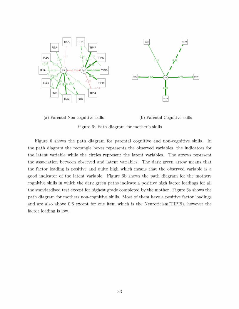
Figure 6: Path diagram for mother’s skills

Figure 6 shows the path diagram for parental cognitive and non-cognitive skills. Inthe path diagram the rectangle boxes represents the observed variables, the indicators forthe latent variable while the circles represent the latent variables. The arrows representthe association between observed and latent variables. The dark green arrow means thatthe factor loading is positive and quite high which means that the observed variable is agood indicator of the latent variable. Figure 6b shows the path diagram for the motherscognitive skills in which the dark green paths indicate a positive high factor loadings for allthe standardised test except for highest grade completed by the mother. Figure 6a shows thepath diagram for mothers non-cognitive skills. Most of them have a positive factor loadingsand are also above 0.6 except for one item which is the Neuroticism(TIPI9), however thefactor loading is low.

33

Latent Factor Indicator Factor Loadings θt Factor Loadings θt+1

Non-cognitive Skills (θNt )

Big FivePersonality(θNb

t )

Extraversion 0.466(-) 0.543(-)Conscientiousness 0.532(0.087) 0.513(0.058)

Neuroticism -0.014(0.089) -0.028(0.060)Openness 0.433(0.075) 0.410(0.054)

Agreeableness 0.384(0.080) 0.403(0.056)Neuroticism (Reversed) 0.505(0.090) 0.477(0.060)

PearlinMastery(θNp

t )

Pearlin Mastery Indicator 1 -0.588(0.226) -0.613(0.108)Pearlin Mastery Indicator 2 -0.568 (0.145) -0.598(0.102)Pearlin Mastery Indicator 3 -0.591(0.132) -0.657(0.102)Pearlin Mastery Indicator 4 0.360(-) 0.414(-)Pearlin Mastery Indicator 5 -0.648 (0.137) -0.676(0.103)Pearlin Mastery Indicator 6 0.362(0.076) 0.4100.054)Pearlin Mastery Indicator 7 -0.549(0.139) -0.539 (0.093)

Neuroticism -0.230(0.244) -0.207(0.176)Cognitive Skills (θCt )

Tests ScoresPIAT Mathematics 0.407(-) 0.418(-)

PIAT Reading Recognition 0.738(0.091) 0.727(0.194)PIAT Reading Comprehension 0.762(0.092) 0.793(0.182)

Table 5: Factor Loadings: Individual’s Non-Cognitive and Cognitive Skills

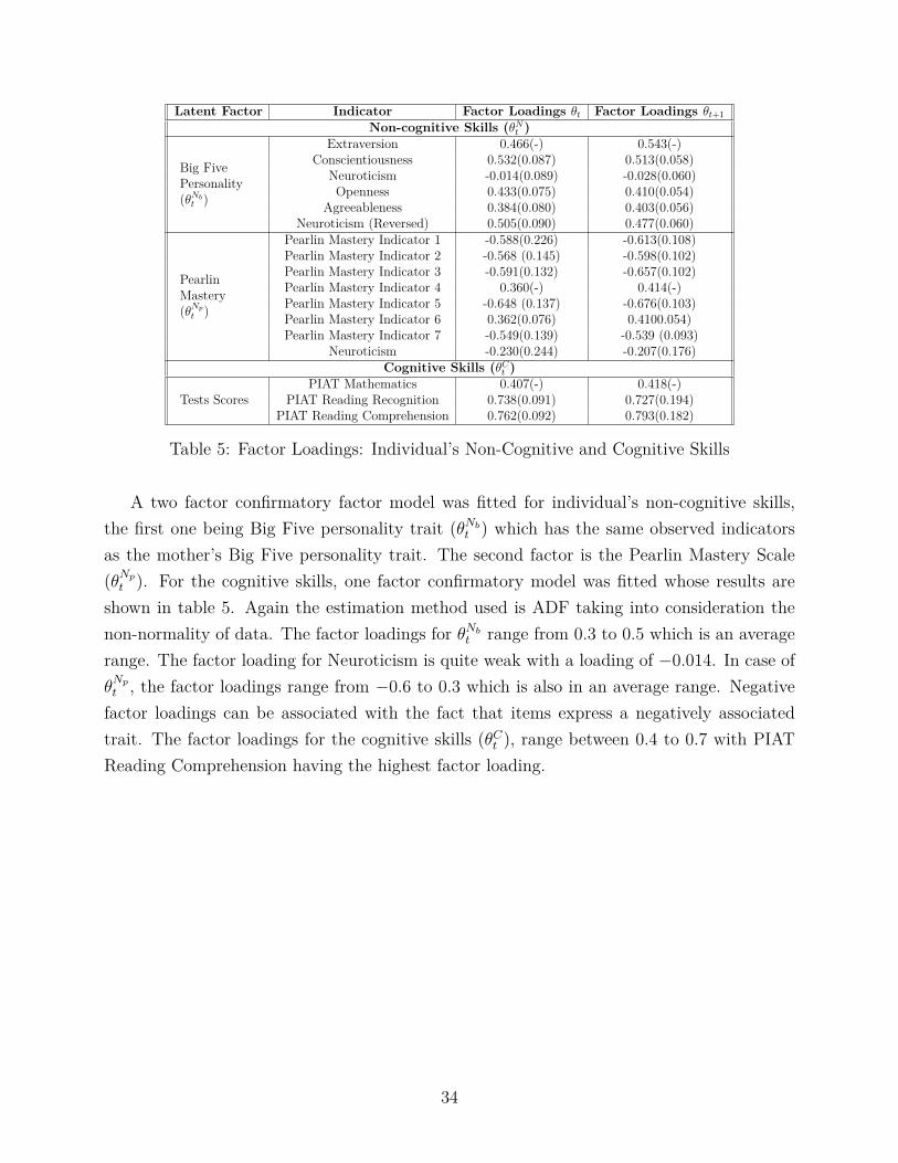
A two factor confirmatory factor model was fitted for individual’s non-cognitive skills,the first one being Big Five personality trait (θNb

t ) which has the same observed indicatorsas the mother’s Big Five personality trait. The second factor is the Pearlin Mastery Scale(θNp

t ). For the cognitive skills, one factor confirmatory model was fitted whose results areshown in table 5. Again the estimation method used is ADF taking into consideration thenon-normality of data. The factor loadings for θNb

t range from 0.3 to 0.5 which is an averagerange. The factor loading for Neuroticism is quite weak with a loading of −0.014. In case ofθNp

t , the factor loadings range from −0.6 to 0.3 which is also in an average range. Negativefactor loadings can be associated with the fact that items express a negatively associatedtrait. The factor loadings for the cognitive skills (θCt ), range between 0.4 to 0.7 with PIATReading Comprehension having the highest factor loading.

34

(a) Cognitive skills (b) Non-Cognitive skills

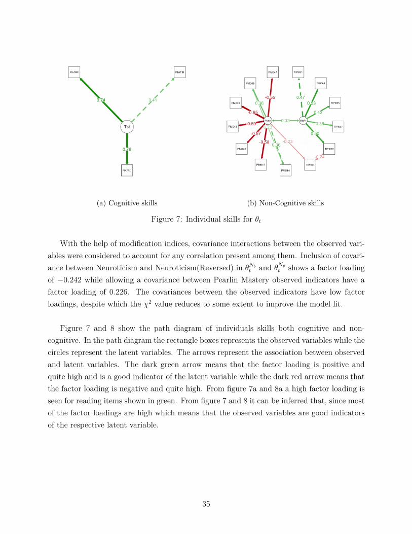
Figure 7: Individual skills for θt

With the help of modification indices, covariance interactions between the observed vari-ables were considered to account for any correlation present among them. Inclusion of covari-ance between Neuroticism and Neuroticism(Reversed) in θNb

t and θNp

t shows a factor loadingof −0.242 while allowing a covariance between Pearlin Mastery observed indicators have afactor loading of 0.226. The covariances between the observed indicators have low factorloadings, despite which the χ2 value reduces to some extent to improve the model fit.

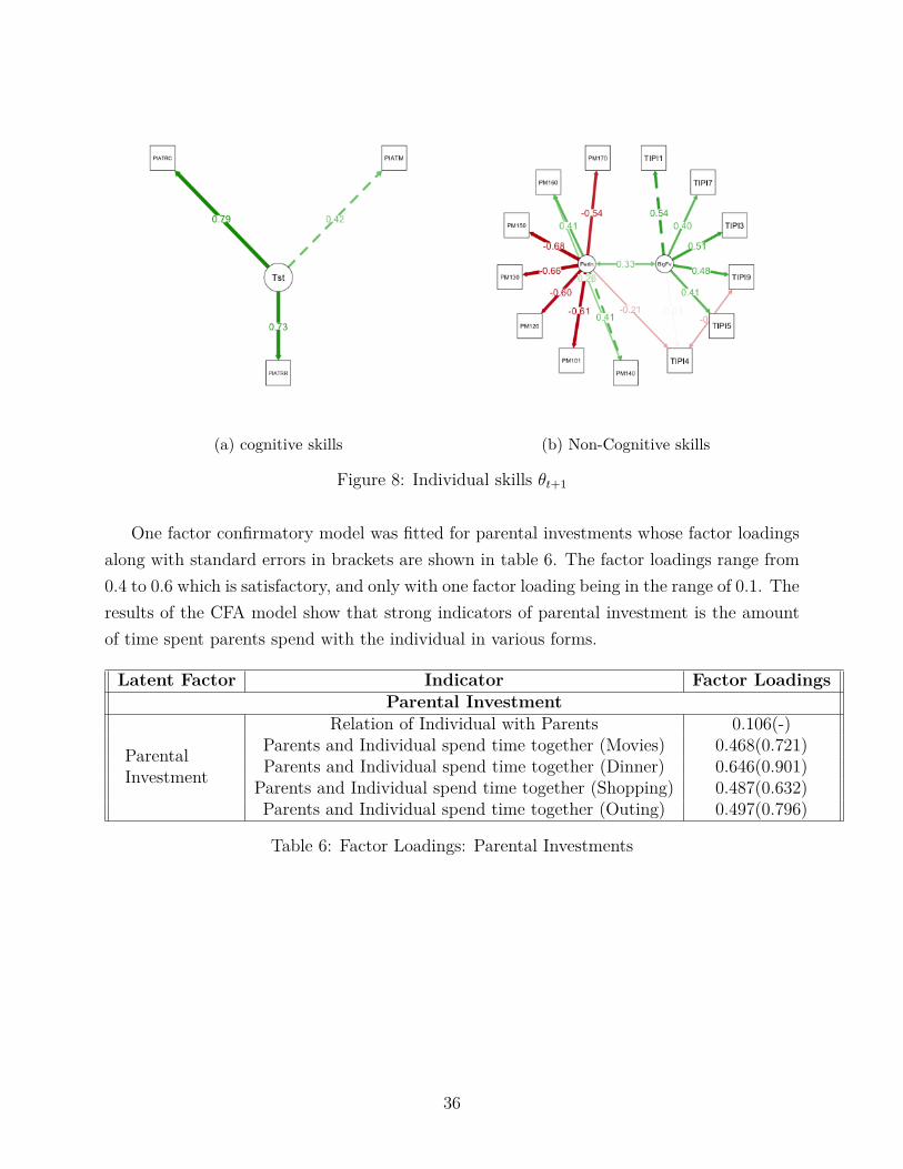
Figure 7 and 8 show the path diagram of individuals skills both cognitive and non-cognitive. In the path diagram the rectangle boxes represents the observed variables while thecircles represent the latent variables. The arrows represent the association between observedand latent variables. The dark green arrow means that the factor loading is positive andquite high and is a good indicator of the latent variable while the dark red arrow means thatthe factor loading is negative and quite high. From figure 7a and 8a a high factor loading isseen for reading items shown in green. From figure 7 and 8 it can be inferred that, since mostof the factor loadings are high which means that the observed variables are good indicatorsof the respective latent variable.

35

(a) cognitive skills (b) Non-Cognitive skills

Figure 8: Individual skills θt+1

One factor confirmatory model was fitted for parental investments whose factor loadingsalong with standard errors in brackets are shown in table 6. The factor loadings range from0.4 to 0.6 which is satisfactory, and only with one factor loading being in the range of 0.1. Theresults of the CFA model show that strong indicators of parental investment is the amountof time spent parents spend with the individual in various forms.

Latent Factor Indicator Factor LoadingsParental Investment

ParentalInvestment

Relation of Individual with Parents 0.106(-)Parents and Individual spend time together (Movies) 0.468(0.721)Parents and Individual spend time together (Dinner) 0.646(0.901)

Parents and Individual spend time together (Shopping) 0.487(0.632)Parents and Individual spend time together (Outing) 0.497(0.796)

Table 6: Factor Loadings: Parental Investments

36

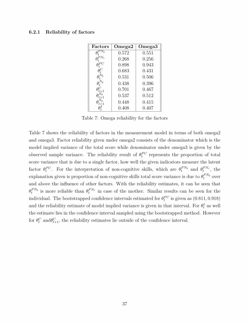
6.2.1 Reliability of factors

Factors Omega2 Omega3θPNbt 0.572 0.551θPNrt 0.268 0.256θPCt 0.898 0.943θCt 0.683 0.431θNbt 0.531 0.506θNp

t 0.438 0.396θCt+1 0.701 0.467θNbt+1 0.537 0.512θNp

t+1 0.448 0.415θIt 0.408 0.407

Table 7: Omega reliability for the factors

Table 7 shows the reliability of factors in the measurement model in terms of both omega2and omega3. Factor reliability given under omega2 consists of the denominator which is themodel implied variance of the total score while denominator under omega3 is given by theobserved sample variance. The reliability result of θPC

t represents the proportion of totalscore variance that is due to a single factor, how well the given indicators measure the latentfactor θPC

t . For the interpretation of non-cognitive skills, which are θPNbt and θPNr

t , theexplanation given is proportion of non-cognitive skills total score variance is due to θPNb

t overand above the influence of other factors. With the reliability estimates, it can be seen thatθPNbt is more reliable than θPNr

t in case of the mother. Similar results can be seen for theindividual. The bootstrapped confidence intervals estimated for θPC

t is given as (0.811, 0.918)and the reliability estimate of model implied variance is given in that interval. For θIt as wellthe estimate lies in the confidence interval sampled using the bootstrapped method. Howeverfor θCt andθCt+1, the reliability estimates lie outside of the confidence interval.

37

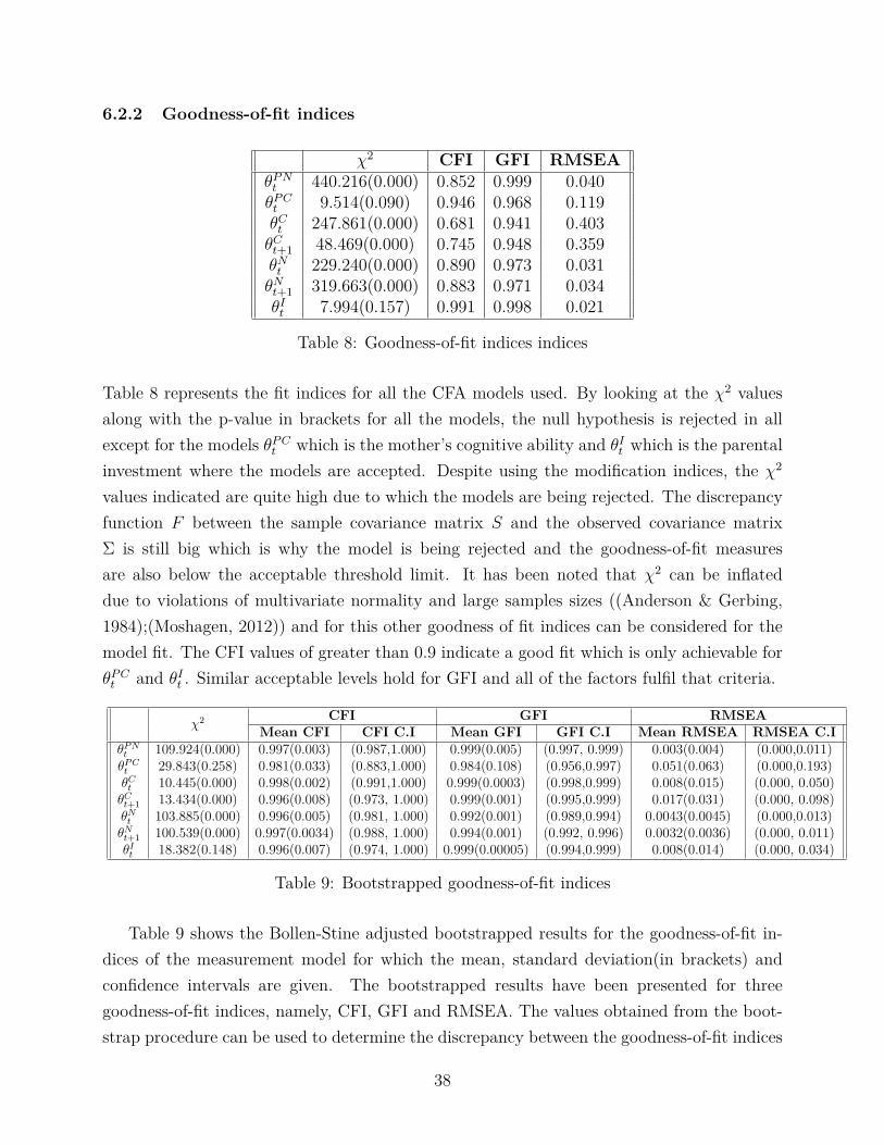
6.2.2 Goodness-of-fit indices

χ2 CFI GFI RMSEAθPNt 440.216(0.000) 0.852 0.999 0.040θPCt 9.514(0.090) 0.946 0.968 0.119θCt 247.861(0.000) 0.681 0.941 0.403θCt+1 48.469(0.000) 0.745 0.948 0.359θNt 229.240(0.000) 0.890 0.973 0.031θNt+1 319.663(0.000) 0.883 0.971 0.034θIt 7.994(0.157) 0.991 0.998 0.021

Table 8: Goodness-of-fit indices indices

Table 8 represents the fit indices for all the CFA models used. By looking at the χ2 valuesalong with the p-value in brackets for all the models, the null hypothesis is rejected in allexcept for the models θPC

t which is the mother’s cognitive ability and θIt which is the parentalinvestment where the models are accepted. Despite using the modification indices, the χ2

values indicated are quite high due to which the models are being rejected. The discrepancyfunction F between the sample covariance matrix S and the observed covariance matrixΣ is still big which is why the model is being rejected and the goodness-of-fit measuresare also below the acceptable threshold limit. It has been noted that χ2 can be inflateddue to violations of multivariate normality and large samples sizes ((Anderson & Gerbing,1984);(Moshagen, 2012)) and for this other goodness of fit indices can be considered for themodel fit. The CFI values of greater than 0.9 indicate a good fit which is only achievable forθPCt and θIt . Similar acceptable levels hold for GFI and all of the factors fulfil that criteria.

χ2 CFI GFI RMSEAMean CFI CFI C.I Mean GFI GFI C.I Mean RMSEA RMSEA C.I

θPNt 109.924(0.000) 0.997(0.003) (0.987,1.000) 0.999(0.005) (0.997, 0.999) 0.003(0.004) (0.000,0.011)θPCt 29.843(0.258) 0.981(0.033) (0.883,1.000) 0.984(0.108) (0.956,0.997) 0.051(0.063) (0.000,0.193)θCt 10.445(0.000) 0.998(0.002) (0.991,1.000) 0.999(0.0003) (0.998,0.999) 0.008(0.015) (0.000, 0.050)θCt+1 13.434(0.000) 0.996(0.008) (0.973, 1.000) 0.999(0.001) (0.995,0.999) 0.017(0.031) (0.000, 0.098)θNt 103.885(0.000) 0.996(0.005) (0.981, 1.000) 0.992(0.001) (0.989,0.994) 0.0043(0.0045) (0.000,0.013)θNt+1 100.539(0.000) 0.997(0.0034) (0.988, 1.000) 0.994(0.001) (0.992, 0.996) 0.0032(0.0036) (0.000, 0.011)θIt 18.382(0.148) 0.996(0.007) (0.974, 1.000) 0.999(0.00005) (0.994,0.999) 0.008(0.014) (0.000, 0.034)

Table 9: Bootstrapped goodness-of-fit indices

Table 9 shows the Bollen-Stine adjusted bootstrapped results for the goodness-of-fit in-dices of the measurement model for which the mean, standard deviation(in brackets) andconfidence intervals are given. The bootstrapped results have been presented for threegoodness-of-fit indices, namely, CFI, GFI and RMSEA. The values obtained from the boot-strap procedure can be used to determine the discrepancy between the goodness-of-fit indices

38

of the actual data and those due to sampling error and hence determine the fit of the model(Bone et al., 1989). The results show a increase in goodness-of-fit as compared to the origi-nal values, indicating a presence of sampling error. Additionally, chi-square values were alsobootstrapped and the relevant p-values were also calculated. In case of the chi-square values,after applying the Bollen-Stine bootstrapping method, the values did reduce substantially,however we still rejected and accepted the same models.

6.3 Part II: Structural Model

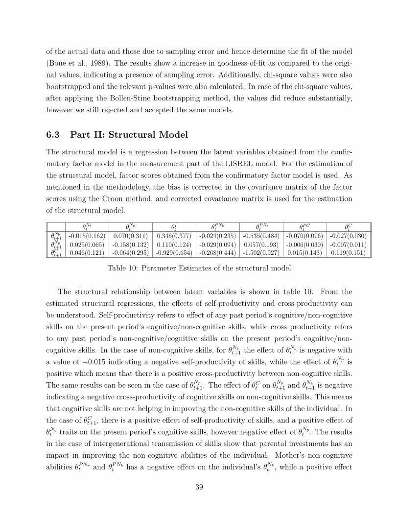
The structural model is a regression between the latent variables obtained from the confir-matory factor model in the measurement part of the LISREL model. For the estimation ofthe structural model, factor scores obtained from the confirmatory factor model is used. Asmentioned in the methodology, the bias is corrected in the covariance matrix of the factorscores using the Croon method, and corrected covariance matrix is used for the estimationof the structural model.

θNbt θ

Np

t θIt θPNbt θPNr

t θPCt θCt

θNbt+1 -0.015(0.162) 0.070(0.311) 0.346(0.377) -0.024(0.235) -0.535(0.484) -0.070(0.076) -0.027(0.030)θNp

t+1 0.025(0.065) -0.158(0.132) 0.119(0.124) -0.029(0.094) 0.057(0.193) -0.006(0.030) -0.007(0.011)θCt+1 0.046(0.121) -0.064(0.295) -0.929(0.654) -0.268(0.444) -1.502(0.927) 0.015(0.143) 0.119(0.151)

Table 10: Parameter Estimates of the structural model

The structural relationship between latent variables is shown in table 10. From theestimated structural regressions, the effects of self-productivity and cross-productivity canbe understood. Self-productivity refers to effect of any past period’s cognitive/non-cognitiveskills on the present period’s cognitive/non-cognitive skills, while cross productivity refersto any past period’s non-cognitive/cognitive skills on the present period’s cognitive/non-cognitive skills. In the case of non-cognitive skills, for θNb

t+1 the effect of θNbt is negative with

a value of −0.015 indicating a negative self-productivity of skills, while the effect of θNp

t ispositive which means that there is a positive cross-productivity between non-cognitive skills.The same results can be seen in the case of θNp

t+1. The effect of θCt on θNp

t+1 and θNbt+1 is negative

indicating a negative cross-productivity of cognitive skills on non-cognitive skills. This meansthat cognitive skills are not helping in improving the non-cognitive skills of the individual. Inthe case of θCt+1, there is a positive effect of self-productivity of skills, and a positive effect ofθNbt traits on the present period’s cognitive skills, however negative effect of θNp

t . The resultsin the case of intergenerational transmission of skills show that parental investments has animpact in improving the non-cognitive abilities of the individual. Mother’s non-cognitiveabilities θPNr

t and θPNbt has a negative effect on the individual’s θNb

t , while a positive effect

39

on the individual’s θNp

t . The intergenerational transmission of cognitive skills has a positiveeffect on the individual’s cognitive ability.

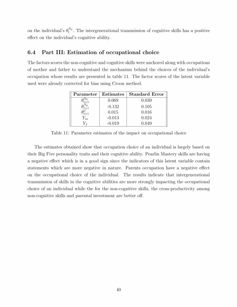
6.4 Part III: Estimation of occupational choice

The factors scores the non-cognitive and cognitive skills were anchored along with occupationsof mother and father to understand the mechanism behind the choices of the individual’soccupation whose results are presented in table 11. The factor scores of the latent variableused were already corrected for bias using Croon method.

Parameter Estimates Standard ErrorθNbt+1 0.069 0.039θNp

t+1 -0.132 0.105θCt+1 0.015 0.016Ym -0.013 0.024Yf -0.019 0.049

Table 11: Parameter estimates of the impact on occupational choice

The estimates obtained show that occupation choice of an individual is largely based ontheir Big Five personality traits and their cognitive ability. Pearlin Mastery skills are havinga negative effect which is in a good sign since the indicators of this latent variable containstatements which are more negative in nature. Parents occupation have a negative effecton the occupational choice of the individual. The results indicate that intergenerationaltransmission of skills in the cognitive abilities are more strongly impacting the occupationalchoice of an individual while the for the non-cognitive skills, the cross-productivity amongnon-cognitive skills and parental investment are better off.

40

7 Discussion & Conclusion

This paper seeks to answer the research question whether there is a presence of intergener-ational transmission of skills in terms of both cognitive and non-cognitive, and its impacton the occupational choice of an individual. The focus was to understand whether parentsskills get transmitted to their offspring and can it help in understanding what factors con-tribute more in an individual making occupational choices which can help in improving thelabor market outcomes. The methodology used for this purpose was Structural EquationModelling(SEM) and the purpose to use this methodology is that certain variables such asnon-cognitive ability are defined as latent variables which are not directly observable andhence they need to be defined from the observed variables. In the measurement model, con-firmatory factor analysis was used to understand how strong are the observed indicators arefor the latent variables. For the non-cognitive skills, the indicators were average while forthe cognitive skills, the indicators were quite high. The average indicators can be explainedby the fact that non-cognitive skills are more of personality traits for which a measurementvalue has not yet been defined. The results in the structural model indicated a positiveeffect of transmission of cognitive skills from mother to the individual, while for the non-cognitive skills it was negative. Instead for the non-cognitive skills, self-productivity andcross-productivity of skills were more dominant along with parental investments. In the finalpart where the latent variables were used to predict the factors contributing to the occu-pational choice of an individual, among the non-cognitive skills, Big Five personality traitsstand out followed by the cognitive skills. This implies that the choice made by an individualto large extent influenced by their underlying personality and their cognitive abilities suchas test scores, GPA, highest grade completed.

One of the limitation was in the estimation of the confirmatory factor model does how-ever reject the null hypothesis with high χ2 value which means that the current hypothesizedmodel is wrong. As discussed in the section 6, the rejection of the models can be due to largesample sizes in which χ2 is sensitive. Despite applying the Bollen-Stine bootstrap procedure,the rejected models were still rejected. For the purpose of the analysis, the model was keptrestricted allowing interactions only between the observed indicators as covariances. Thiscould be one of the reasons for the rejection of the models. However, when more interactionswere allowed between the latent variables, the factor loadings became weak. There was atradeoff between the model significance and factor loadings which was consecutively used forfurther analysis of the model. Moreover, in the case of non-cognitive skills, which are person-ality traits model significance can be tough to achieve. The models for parental investment

41

and mother’s cognitive skills were however accepted which could be due to low sample sizepresent in them.

Another limitation was the availability of the dataset of the father’s cognitive and non-cognitive skills which allowed only the estimation of mother’s skills. The analysis could onlyanswer the transmission of mother’s skills to the individual which showed that mother’s cog-nitive ability positively affects the individual’s cognitive ability influencing the occupationalchoice of the individual. Further, for the estimation of the structural model, instead of usingthe factor scores, the model could have been estimated implicitly but it did lead to error asthe inverse of the covariance matrix was singular. The reliability of the measurement modeldiffers in terms of the model implied variance and observed sample variance. The reliabilitybased on the model implied variance gives a higher reliability factor than the observed samplevariance from which it can be inferred that the model can be relied, however, the presenceof model misspecification cannot be completely ruled out.

The paper does present econometric challenges in terms of the rejection of models, av-erage factor loadings in the measurement model, possible presence of misspecification in themeasurement model. However, given that all of the variables under consideration are latentvariables most of which are personality traits since these variables are not of quantifiablenature, econometric challenges are more likely to occur. For further research, the existingmodel could be expanded more to include more observed variables such as race, ethnicity,income of parents, effect of siblings, and other varied background. This can potentially helpin reducing any potential model misspecification as well. In the empirical economics litera-ture non-cognitive skills are often termed as black box which has become research interest ofmany even in terms of improving econometric estimation techniques for them. Opening upthese black boxes, can help in improvement of educational programs, job market preparednesswhich can overall improve the quality of life of an individual.

42

References

Anderson, J. C., & Gerbing, D. W. (1984). The effect of sampling error on convergence,improper solutions, and goodness-of-fit indices for maximum likelihood confirmatoryfactor analysis. Psychometrika, 49 (2), 155–173.

Anderson, J. C., & Gerbing, D. W. (1988). Structural equation modeling in practice: Areview and recommended two-step approach. Psychological bulletin, 103 (3), 411.

Anger, S. (2012). The intergenerational transmission of cognitive and non-cognitive skillsduring adolescence and young adulthood.

Anger, S., & Heineck, G. (2010). Do smart parents raise smart children? the intergenerationaltransmission of cognitive abilities. Journal of population Economics, 23 (3), 1105–1132.

Asparouhov, T., & Muthén, B. (2009). Exploratory structural equation modeling. Structuralequation modeling: a multidisciplinary journal, 16 (3), 397–438.

Bearden, W. O., Sharma, S., & Teel, J. E. (1982). Sample size effects on chi square andother statistics used in evaluating causal models. Journal of marketing research, 19 (4),425–430.

Becker, G. S. (2009). Human capital: A theoretical and empirical analysis, with specialreference to education. University of Chicago press.

Benson, J., & Fleishman, J. A. (1994). The robustness of maximum likelihood anddistribution-free estimators to non-normality in confirmatory factor analysis. Qual-ity and Quantity, 28 (2), 117–136.

Bentler, P. M., & Dudgeon, P. (1996). Covariance structure analysis: Statistical practice,theory, and directions. Annual review of psychology, 47 (1), 563–592.

Bollen, K. A. (1996). An alternative two stage least squares (2sls) estimator for latentvariable equations. Psychometrika, 61 (1), 109–121.

Bollen, K. A., & Stine, R. A. (1992). Bootstrapping goodness-of-fit measures in structuralequation models. Sociological Methods & Research, 21 (2), 205–229.

Bone, P. F., Sharma, S., & Shimp, T. A. (1989). A bootstrap procedure for evaluatinggoodness-of-fit indices of structural equation and confirmatory factor models. Journalof Marketing Research, 26 (1), 105–111.

Brown, T. A., & Moore, M. T. (2012). Confirmatory factor analysis. Handbook of structuralequation modeling, 361–379.

Browne, M. W. (1982). Covariance structures. Topics in applied multivariate analysis,72–141.

Brunello, G., & Schlotter, M. (2011). Non-cognitive skills and personality traits: Labourmarket relevance and their development in education & training systems.

43

Burt, R. S. (1976). Interpretational confounding of unobserved variables in structural equa-tion models. Sociological methods & research, 5 (1), 3–52.

Chamberlain, G. (1982). Multivariate regression models for panel data. Journal of econo-metrics, 18 (1), 5–46.

Chevalier, A., et al. (2002). Just like daddy: the occupational choice of uk graduates. InRoyal economic society annual conference 2002.

Chin, W. W. (1998). Commentary: Issues and opinion on structural equation modeling.JSTOR.

Cobb-Clark, D. A., & Tan, M. (2011). Noncognitive skills, occupational attainment, andrelative wages. Labour Economics, 18 (1), 1–13.

Constant, A. F., & Zimmermann, K. F. (2003). Occupational choice across generations.Available at SSRN 487416 .

Croon, M. (2002). Using predicted latent scores in general latent structure models. LatentVariable and Latent Structure Models, 195–224.

Cubel, M., Nuevo-Chiquero, A., Sanchez-Pages, S., & Vidal-Fernandez, M. (2016). Dopersonality traits affect productivity? evidence from the laboratory. The EconomicJournal, 126 (592), 654–681.

Cunha, F., & Heckman, J. J. (2008). Formulating, identifying and estimating the technologyof cognitive and noncognitive skill formation. Journal of human resources, 43 (4), 738–782.

de Coulon, A., Meschi, E., & Vignoles, A. (2011). Parents’ skills and children’s cognitiveand non-cognitive outcomes. Education economics, 19 (5), 451–474.

Devlieger, I., & Rosseel, Y. (2017). Factor score path analysis. Methodology.Ham, R., Junankar, P. N., & Wells, R. (2009a). Antagonistic managers, careless workers

and extraverted salespeople: an examination of personality in occupational choice.Ham, R., Junankar, P. N., & Wells, R. (2009b). Occupational choice: Personality matters

(Tech. Rep.). IZA discussion papers.Heckman, J. J., Lochner, L. J., & Todd, P. E. (2003). Fifty years of mincer earnings

regressions (Tech. Rep.). National Bureau of Economic Research.Heckman, J. J., & Rubinstein, Y. (2001). The importance of noncognitive skills: Lessons

from the ged testing program. American Economic Review, 91 (2), 145–149.Heckman, J. J., Stixrud, J., & Urzua, S. (2006). The effects of cognitive and noncognitive

abilities on labor market outcomes and social behavior. Journal of Labor economics,24 (3), 411–482.

Joereskog, K., & Sörbom, D. (1984). Analysis of linear structural relations by maximumlikelihood, instrumental variables, and least squares methods, users guide. Uppsala:

44

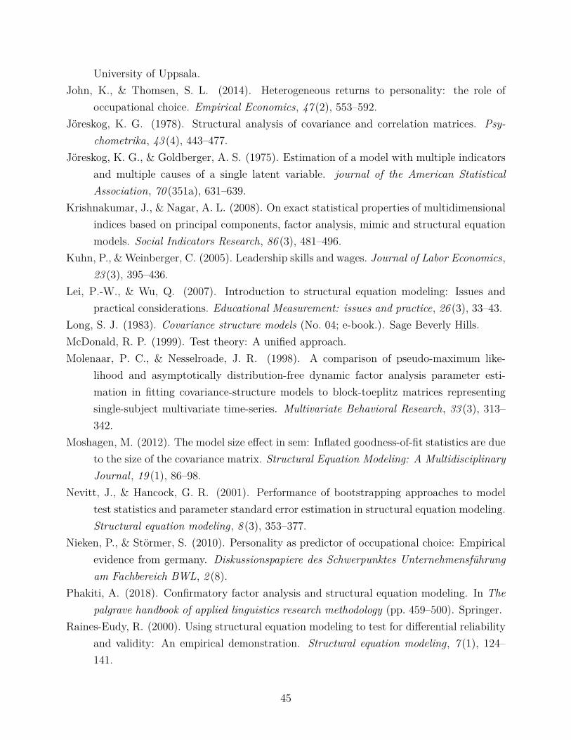
University of Uppsala.John, K., & Thomsen, S. L. (2014). Heterogeneous returns to personality: the role of

occupational choice. Empirical Economics, 47 (2), 553–592.Jöreskog, K. G. (1978). Structural analysis of covariance and correlation matrices. Psy-

chometrika, 43 (4), 443–477.Jöreskog, K. G., & Goldberger, A. S. (1975). Estimation of a model with multiple indicators

and multiple causes of a single latent variable. journal of the American StatisticalAssociation, 70 (351a), 631–639.

Krishnakumar, J., & Nagar, A. L. (2008). On exact statistical properties of multidimensionalindices based on principal components, factor analysis, mimic and structural equationmodels. Social Indicators Research, 86 (3), 481–496.

Kuhn, P., & Weinberger, C. (2005). Leadership skills and wages. Journal of Labor Economics,23 (3), 395–436.

Lei, P.-W., & Wu, Q. (2007). Introduction to structural equation modeling: Issues andpractical considerations. Educational Measurement: issues and practice, 26 (3), 33–43.

Long, S. J. (1983). Covariance structure models (No. 04; e-book.). Sage Beverly Hills.McDonald, R. P. (1999). Test theory: A unified approach.Molenaar, P. C., & Nesselroade, J. R. (1998). A comparison of pseudo-maximum like-

lihood and asymptotically distribution-free dynamic factor analysis parameter esti-mation in fitting covariance-structure models to block-toeplitz matrices representingsingle-subject multivariate time-series. Multivariate Behavioral Research, 33 (3), 313–342.

Moshagen, M. (2012). The model size effect in sem: Inflated goodness-of-fit statistics are dueto the size of the covariance matrix. Structural Equation Modeling: A MultidisciplinaryJournal, 19 (1), 86–98.

Nevitt, J., & Hancock, G. R. (2001). Performance of bootstrapping approaches to modeltest statistics and parameter standard error estimation in structural equation modeling.Structural equation modeling, 8 (3), 353–377.

Nieken, P., & Störmer, S. (2010). Personality as predictor of occupational choice: Empiricalevidence from germany. Diskussionspapiere des Schwerpunktes Unternehmensführungam Fachbereich BWL, 2 (8).

Phakiti, A. (2018). Confirmatory factor analysis and structural equation modeling. In Thepalgrave handbook of applied linguistics research methodology (pp. 459–500). Springer.

Raines-Eudy, R. (2000). Using structural equation modeling to test for differential reliabilityand validity: An empirical demonstration. Structural equation modeling, 7 (1), 124–141.

45

Raykov, T. (1998). A method for obtaining standard errors and confidence intervals ofcomposite reliability for congeneric items. Applied Psychological Measurement, 22 (4),369–374.

Schreiber, J. B., Nora, A., Stage, F. K., Barlow, E. A., & King, J. (2006). Reportingstructural equation modeling and confirmatory factor analysis results: A review. TheJournal of educational research, 99 (6), 323–338.

Schumacker, E., & Lomax, G. (2016). A beginner’s guide to structural equation modeling.4th edtn. New York, NY: Routledge.

Shanmugam, V., & Marsh, J. (2015). Application of structural equation modeling to thesocial sciences: a brief guide for researchers. Mesure et évaluation en éducation, 37 (3),99–123.

Skrondal, A., & Laake, P. (2001). Regression among factor scores. Psychometrika, 66 (4),563–575.

Todd, P. E., & Zhang, W. (2020). A dynamic model of personality, schooling, and occupa-tional choice. Quantitative Economics, 11 (1), 231–275.

Tsai, J. (2006). Decoding the ged signal: Labor market returns to non-cognitive ability(graduate seminar draft).

Viladrich, C., Angulo-Brunet, A., & Doval, E. (2017). A journey around alpha and omegato estimate internal consistency reliability. Annals of Psychology, 33 (3), 755–782.

Weston, R., & Gore Jr, P. A. (2006). A brief guide to structural equation modeling. Thecounseling psychologist, 34 (5), 719–751.

World Economic Forum. (2021). Building a common language for skills at work a globaltaxonomy.

Yuan, K.-H., & Bentler, P. M. (1997). Mean and covariance structure analysis: Theoreticaland practical improvements. Journal of the American statistical association, 92 (438),767–774.

46

8 Appendix

The list of Pearlin Mastery Indicators:

• Pearlin Mastery 1: No way I can solve the problems I have

• Pearlin Mastery 2: I sometimes feel that I am being pushed around

• Pearlin Mastery 3: I sometimes feel that I am being pushed around

• Pearlin Mastery 4: I can do just about anything that happens in my life

• Pearlin Mastery 5: I often feel helpless in dealing problems in my life

• Pearlin Mastery 6: What happens to me in future mostly depends on me

• Pearlin Mastery 7: Little I can do to change things in my life

The Rotter Locus of Control indicators is as follows:

• Rotter Locus of Control Indicator 1: Degree of control individual has over direction ofown life

• Rotter Locus of Control Indicator 2: Is the above statement much or slightly closer toindividual’s opinion?

• Rotter Locus of Control Indicator 3: Importance of Planning

• Rotter Locus of Control Indicator 4: Is the above statement much or slightly closer toindividual’s opinion?

• Rotter Locus of Control Indicator 5: Importance of Luck

• Rotter Locus of Control Indicator 6: Is the above statement much or slightly closer toindividual’s opinion?

• Rotter Locus of Control Indicator 7: Degree of Influence R has over own life

• Rotter Locus of Control Indicator 8: Is the above statement much or slightly closer toindividual’s opinion?

47

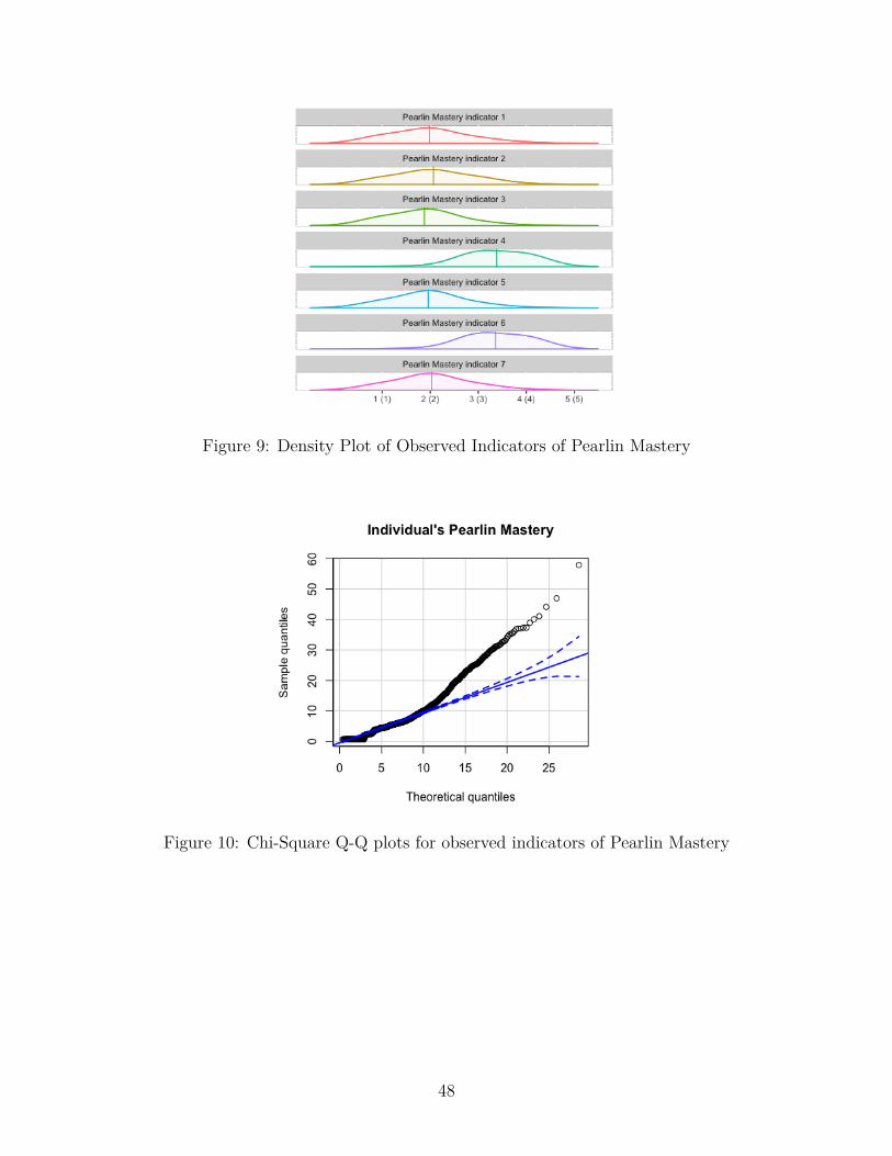
Figure 9: Density Plot of Observed Indicators of Pearlin Mastery

Figure 10: Chi-Square Q-Q plots for observed indicators of Pearlin Mastery

48