Embed Size (px)
Citation preview
DI
SC
US
SI
ON
P
AP
ER
S
ER
IE
S
Forschungsinstitut zur Zukunft der ArbeitInstitute for the Study of Labor
Intergenerational Income Mobility in Urban China
IZA DP No. 4811
March 2010
Cathy Honge GongAndrew LeighXin Meng
Intergenerational Income Mobility
in Urban China
Cathy Honge Gong University of Canberra
Andrew Leigh
Australia National University and IZA
Xin Meng
Australia National University and IZA
Discussion Paper No. 4811 March 2010
IZA
P.O. Box 7240 53072 Bonn
Germany
Phone: +49-228-3894-0 Fax: +49-228-3894-180
E-mail: [email protected]
Any opinions expressed here are those of the author(s) and not those of IZA. Research published in this series may include views on policy, but the institute itself takes no institutional policy positions. The Institute for the Study of Labor (IZA) in Bonn is a local and virtual international research center and a place of communication between science, politics and business. IZA is an independent nonprofit organization supported by Deutsche Post Foundation. The center is associated with the University of Bonn and offers a stimulating research environment through its international network, workshops and conferences, data service, project support, research visits and doctoral program. IZA engages in (i) original and internationally competitive research in all fields of labor economics, (ii) development of policy concepts, and (iii) dissemination of research results and concepts to the interested public. IZA Discussion Papers often represent preliminary work and are circulated to encourage discussion. Citation of such a paper should account for its provisional character. A revised version may be available directly from the author.
IZA Discussion Paper No. 4811 March 2010
ABSTRACT
Intergenerational Income Mobility in Urban China* This paper estimates the intergenerational income elasticity for urban China, paying careful attention to the potential biases induced by income fluctuations and life cycle effects. Our preferred estimates are that the intergenerational income elasticities are 0.74 for father-son, 0.84 for father-daughter, 0.33 for mother-son, and 0.47 for mother-daughter. This suggests that while China has experienced rapid growth of absolute incomes, the relative position of children in the distribution is largely determined by their parents’ incomes. Investigating possible causal channels, we find that parental education, occupation, and Communist Party membership all play important roles in transmitting economic status from parents to children. JEL Classification: D10, D31 Keywords: intergenerational mobility, transgenerational persistence,
political party membership Corresponding author: Xin Meng Division of Economics Research School of Economics Australian National University Canberra 0200 Australia E-mail: [email protected]
* We are grateful to Mario Fiorini, Bob Gregory, Michael Schneider, and participants at the 12th Annual Labour Econometrics Workshop and an Australian National University conference on ‘The Economics of Intergenerational Mobility’ for valuable comments on earlier drafts. Jenny Chesters provided outstanding research assistance.
Intergenerational Income Mobility in Urban China
1. Introduction
Economists have long been interested in the issue of intergenerational mobility.
Estimating the relationship between the permanent incomes of parents and children is a
critical component of a society’s income dynamics. A growing body of research has
demonstrated large and systematic differences across nations, with parental income being
a major determinant of children’s incomes in some countries, and much less important in
others. To date, much of the existing research on intergenerational mobility has focused
on developed nations. While this has the advantage that data sources are generally more
reliable, developed nations also tend to be politically stable and to have experienced
modest rates of growth.
By contrast, the growth experience of China over the past three decades has been
nothing short of unprecedented. As the world’s most populous nation, Chinese living
standards have risen six-fold since 1979. These rapid economic changes have also been
accompanied by dramatic social transformations. All this makes China a unique case
study through which to better understand the relationship between societal change and
income mobility.
In traditional Chinese society (prior to 1949), most social welfare was familial.
There was a strong reciprocal relationship between parents and children. Parents
normally invested a large proportion of their income and assets in their offspring’s
education and career development (and the parental social network played an important
role in children’s access to education and the labour market). Children typically lived
with their parents until marriage (and in many cases, after marriage as well). In return,
parents expected their children to support them in old age.
During the Maoist era (1949-77), social welfare was universally provided in urban
areas, with the aim of making Chinese society more egalitarian. By and large, this
successfully compressed the distribution of income and wealth over the Maoist period
(Meng 2004, 2007; Benjamin, Brandt, Giles and Wang, 2005). In addition, the early
socialist revolution attempted to weaken the social ties between parental and children’s
1
occupations by making it impossible for children to inherit any meaningful wealth from
their parents, and opening up better opportunities for education and occupational
attainment for the children of poor families (Cheng and Dai 1995). These might have
facilitated an increase in intergenerational income mobility.
However, close family ties still exist and continue to deliver economic and social
advantages from one generation to another. Indeed, some government policies have even
decreased mobility. For instance, the policies of intergenerational job replacement (Dingti)
and internal recruitment (Neizhao), which were introduced in 1977 and then were to be
abolished in 1986, might have reduced the level of mobility in urban China (Yu and Liu,
2004).4 In addition, the unique household registration system initiated in Mao’s era
restricted geographic labor mobility, and therefore probably reduced intergenerational
mobility (Wu and Treiman, 2003).5
The transition from a planned to a market oriented economy initiated in the late
1970s and early 1980s has moved the society away from the social provision of welfare
back towards one that relies heavily upon individual and family responsibilities (Cai,
Giles and Meng, 2006). As a consequence, income/wealth inequality has increased
sharply and family networks play an important role in job attainment, which, in turn, may
have resulted in falling inter-generational income mobility. In the meantime, a steady
increase in geographic mobility may have boosted intergenerational mobility across
China as a whole (Wu and Treiman, 2003; Yu and Liu, 2004; Takenoshita, 2007).6
4 Yu and Liu (2004) find that since 1978, the sector, rank and size of parents’ work unit have had significant effects on that their children’s first job, and this effect did not attenuate even after 1986 when these two policies were abolished.
5 In Mao’s era, China’s unique household registration system restricted people in rural areas or small cities from accessing better opportunities in urban areas or large cities. They could only move permanently across regions by applying for permission, achieving tertiary education, getting military experience, or being recruited into a state-owned enterprise. Under the household registration system, most parents and children would locate in a same city. The intergenerational persistence in locality enhanced the intergenerational persistence in education and labor market outcomes due to systematic regional disparities in educational quality and labor markets.
6 Since China’s post-1978 economic reforms, the household registration system was gradually relaxed, with permission no longer required for temporary moves across regions, and local registration no longer needed in order to acquire an informal job or to run an individual business. However, to access the jobs in the formal sector, or to permanently change their registration, people still require tertiary education, military experience or sufficient capital.
2
A few studies on intergenerational mobility in China appear mainly in the
sociological literature. These generally focus on social stratification and political
affiliation. Such studies mainly concentrate on occupational mobility and find strong
intergenerational transmission in occupations and industries (Lin and Bian, 1991; Cheng
and Dai 1995; Takenoshita, 2007). In general, Communist Party members and state
employees (especially government officials) have many social advantages in obtaining
entrance into university, or locating better job opportunities for their children (Lin and
Bian, 1991; Walder, Li and Treiman, 2000; Bian, 2002; Meng, 2007).
The only other study on intergenerational income mobility in urban China is Guo
and Min (2008), who uses the Chinese Urban Household Education and Employment
Survey 2004 (UHEES 2004). They estimate the overall intergenerational income
elasticity in urban China to be 0.32 (for fathers and sons) and find that education has
played an important role in promoting intergenerational income mobility. However, their
study uses only one income observation for parents, and one income observation for
children. We aim to advance on this work by accounting for life cycle variation of
income, and exploring the possible role of parental social status in determining children’s
outcomes.
This paper combines UHEES 2004 with repeated cross-sectional datasets
covering nearly 20 years. To preview our results, we find a much higher intergenerational
income elasticity than the previous estimates by Guo and Min (2008). After accounting for
fluctuations in parents’ incomes and life cycle variation in children’s incomes, we
estimate that the intergenerational elasticity in urban China is around 0.74 for father-son,
0.84 for father-daughter, 0.33 for mother-son, and 0.47 for mother-daughter. This is an
extremely high level of intergenerational persistence, and implies that intergenerational
mobility is much lower in China than in most developed nations. Exploring the channels
through which income is transmitted across generations, we conclude that parental education,
occupation, industry, and Communist Party membership all play important roles in
transmitting economic status from parents to children.
The paper is structured as follows. Section 2 reports the methodology on how to
estimate intergenerational income elasticity. Section 3 describes the data and summarizes
3
the statistics. Section 4 presents estimates of intergenerational income and earnings
elasticities. Section 5 explores the main channels through which income is transmitted
from parents to children. The final section concludes.
2. Methodology
Studies of intergenerational mobility generally estimate the association between
the socioeconomic status of parents and their offspring. Becker and Tomes (1979) first
suggested a log-linear intergenerational income regression to estimate the
intergenerational elasticity.
ipici yy εβα ++= , (1)
where ciy is the log of children’s income, piy is the log of parents’ income. The
coefficient β is the intergenerational income elasticity. The larger the elasticity, the less
mobility in a given society.
Ideally, intergenerational mobility calculations should estimate the elasticity of
lifetime income between children and parents.7 Using just one year’s earnings/income
data for parents and children can lead to a significant underestimate of the true lifetime
intergenerational elasticity (Solon, 1992; Mazumder, 2005; Haider and Solon, 2006;
Bohlmark and Lindquist, 2006; Dunn, 2007).8
In order to deal with the measurement error from using one year earnings/income
to proxy for lifetime earnings/income, previous studies take an average of income over a
number of different years for parents in order to obtain a better estimate of permanent
income (Solon, 1992; Lee and Solon, 2006; Nicoletti and Ermisch, 2007). However,
Mazumder (2005) argues that the transitory component of income is highly persistent and
even a five year average may still provide a rather poor measurement of permanent
income. 7 In theory, one might argue that what should be important is not a parent’s lifetime income, but the amount of resources available in the household during the years when the child was growing up. In practice, most researchers have typically regarded this issue as being less important than obtaining a stable measure of parental income or earnings. 8 For instance, Dunn (2007) finds that in Brazil, the intergenerational earnings elasticity grows sharply with son’s age, reaching a maximum for sons aged 49, before falling slightly as son’s age increases further. Father’s age is found to have much less effect on mobility estimates than the son’s age and the use of father’s age over 40 produces quite stable elasticity estimates.
4
Although measurement error in the dependent variable does not in itself lead to
attenuation bias, Haider and Solon (2006) point out that a attenuation bias can be caused
by using log current earnings when children are in their twenties (a point at which current
earnings may be quite different from average lifetime earnings). This error can be
minimized by using log current earnings measured when children are aged in their thirties
or forties (a point at which current earnings are close to average lifetime earnings).
To address these issues, prior researchers have controlled for the age of both
children and parents, averaging parental income over multiple years, or predicting
parental lifetime income by instrumenting income using parental characteristics (Reville,
1995; Dearden, Machin and Reed, 1997; Bjoklund and Jantti, 1997; Fortin and Lefebvre,
1998; Grawe, 2001; Chadwick and Solon , 2002; Mazumder, 2005; Lefranc and Trannoy,
2005; Haider and Solon, 2006; Grawe, 2006; Ferreira and Veloso, 2006; Lee and Solon,
2006, Nicoletti and Ermisch, 2007; Herz et al., 2007; Mocetti, 2007; Dunn, 2007; Leigh,
2007). However, a key issue in the instrumental variable approach is selecting
instruments that only affect children’s earnings through the channel of parental earnings,
and do not directly impact children’s earnings (Solon, 1992).
In addition to general issues that arise when estimating intergenerational
elasticities, the specific economic environment in China over recent decades may also
pose additional difficulty in estimating parental lifetime income. Due to rapid economic
growth and sectoral change, the age-earnings profile and the return to particular
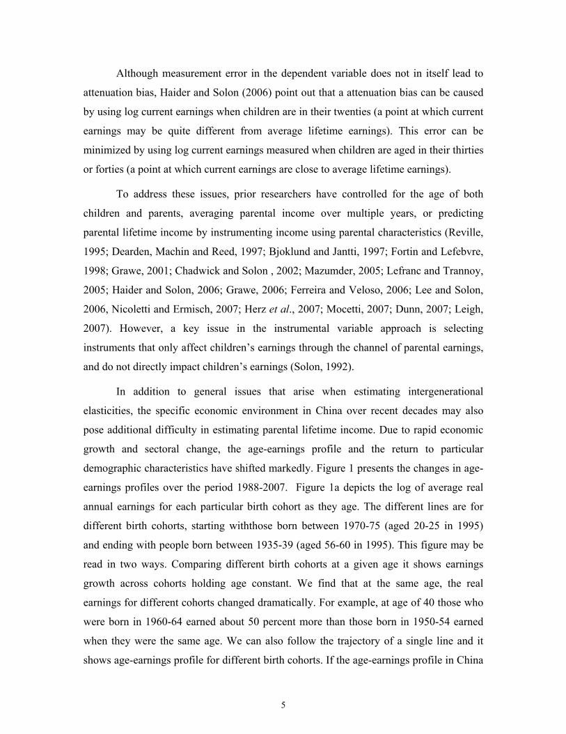
demographic characteristics have shifted markedly. Figure 1 presents the changes in age-
earnings profiles over the period 1988-2007. Figure 1a depicts the log of average real
annual earnings for each particular birth cohort as they age. The different lines are for
different birth cohorts, starting withthose born between 1970-75 (aged 20-25 in 1995)
and ending with people born between 1935-39 (aged 56-60 in 1995). This figure may be
read in two ways. Comparing different birth cohorts at a given age it shows earnings
growth across cohorts holding age constant. We find that at the same age, the real
earnings for different cohorts changed dramatically. For example, at age of 40 those who
were born in 1960-64 earned about 50 percent more than those born in 1950-54 earned
when they were the same age. We can also follow the trajectory of a single line and it
shows age-earnings profile for different birth cohorts. If the age-earnings profile in China
5
had remained constant, one would expect to see the the shape of the lines remaining
parallel to one another. Instead, it is evident that earnings growth has affected the wage
profile differentially for different cohorts. For example, for those born in 1950-54 the
profile did not flatten out untilage 50, whereas for those born between 1960-64, the
profile started to flatten out when they turned 38.
Another way to illustrate the same point is to look at age-earnings profiles over
time. Figure 1b takes the average real earnings ratios for each age between 1988 and
1995, 1995 and 2000, and 2000 and 2007. If there is no change in the shape of the age-
earnings profile, the graph should show horizontal lines. Figure 1b indicates that between
1988 and 1995, real earnings rose for workers in their 30s, but fell for workers in their
60s. This was partly reversed between 1995 and 2000 (when workers in their 50s and 60s
enjoyed the most rapid earnings growth). In the period 2000−2007, prime-aged workers
again experienced more rapid growth in real earnings than their older and younger
counterparts).
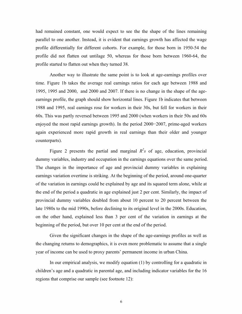
Figure 2 presents the partial and marginal R2s of age, education, provincial
dummy variables, industry and occupation in the earnings equations over the same period.
The changes in the importance of age and provincial dummy variables in explaining
earnings variation overtime is striking. At the beginning of the period, around one-quarter
of the variation in earnings could be explained by age and its squared term alone, while at
the end of the period a quadratic in age explained just 2 per cent. Similarly, the impact of
provincial dummy variables doubled from about 10 percent to 20 percent between the
late 1980s to the mid 1990s, before declining to its original level in the 2000s. Education,
on the other hand, explained less than 3 per cent of the variation in earnings at the
beginning of the period, but over 10 per cent at the end of the period.
Given the significant changes in the shape of the age-earnings profiles as well as
the changing returns to demographics, it is even more problematic to assume that a single
year of income can be used to proxy parents’ permanent income in urban China.
In our empirical analysis, we modify equation (1) by controlling for a quadratic in
children’s age and a quadratic in parental age, and including indicator variables for the 16
regions that comprise our sample (see footnote 12):
6
ici2
pi2pi12ci2ci1pici RAAAAyy εδγγϕϕβα +++++++= , (2)
where ciy is the log of the child’s observed income, piy is the log of the parent’s observed
income, ciA is the child’s age minus 40 (and 2ciA is its square), piA is the parent’s age (and
2piA is its square). ciR is a vector of regional dummy variables capturing regional variation
in prices and wages.
In our first specification, we use OLS to estimate equation (2), and restrict the age
range for children and parents to an interval where current earnings are the best proxy for
long-run earnings (we also experiment with varying this age range).9
Our second specification aims to address the potential downward bias caused by
mis-measurement of parental income by instrumenting reported parental income with
parental education.10 This method, however, may suffer from certain weaknesses. If the
rate of return to human capital changes significantly over time, as has occurred in China
(Meng and Kidd, 1997; Zhang, Zhao, Park, and Song, 2005; and Meng, Shen, and Xue,
2009), we will mis-estimate different cohorts’ lifetime income. Another problem is
parental education may have an independent effect on children’s income (Solon, 1992).
For example, nepotism in the Chinese university admissions process might lead us to
overestimate the true intergenerational income elasticity if we instrument using parental
education. Similarly, nepotism in the Chinese job market might lead us to overestimate
the true intergenerational income elasticity if we instrument using parental occupation.
Our third approach, following Arellano and Meghir (1992), Angrist and Krueger
(1992), Bjorklund and Jantti (1997), Mocetti (2007), and Nicoletti and Ermisch (2007) is
to adopt the method of two-sample two-stage-least-squares (TS2SLS). To implement this,
we use the cross sectional survey (UHEES 2004) containing information on both
children’s and parents’ current income, education, and demographics. We then combine
this with repeated cross-sectional data covering a two-decade period, and include
information about parental pseudo-cohorts’ earnings, education, occupation, and actual
9 Although we are guided in this analysis by the work of Haider and Solon (2006), their empirical analysis uses U.S. data, and therefore considers an economy with a relatively stable wage growth and age-earnings profile. The situation for China is different. As indicated in Figure 1a, over time the age-earnings profile has changed markedly, with 30-45 year olds experiencing more rapid wage increases than other age groups. 10 To test sensitivity of the instrument we also use parental occupation and industry of employment as instruments to predict their permanent income.
7
labour market experience. We predict parental permanent income using the latter data
source, hoping that it will allow us to better proxy parental permanent income over a
period of significant income changes.
To be precise, we use the repeated cross-section sample to estimate the following
equation separately for each gender and year over the period 1986-2004:
itititit vovPrXy +++= ηβα (3)
where ity is the log of observed real income (deflated by province-specific price indices)
for individuals who are of working age (men aged 16 to 60 and women aged 16 to 55)
and working in year t, Xi is a vector of individual characteristics including years of
schooling, actual age and its square term in year t, while itovPr is a vector of provincial
dummies. Since the second stage equation also includes parental age and a vector of
provincial dummies, the excluded instrument is parental education. We also repeat the
same exercise using occupation and industry of employment as the instruments.
Based on the estimated coefficients from Equation (3) and parental demographics
from the survey that contains information on parents and children, we then predict
parental income year by year for the period 1986-2004.11 After doing so, we calculate
each individual’s average earnings taking away the time trend. Only the sample of
individuals who have at least 5 consecutive years of predicted parental income are
included.
In addition to the benefit of better capturing parental permanent income, this
method also significantly increases the number of observations with both children and
parental incomes. However, this method does not avoid the problem of violating the
exclusion restriction. Hence, when interpreting the results we should bear this in mind.
11 The age of the parents for the year t-n for the prediction is calculated by ( nAA tnt −=− ). Because we have information from the parent-child dataset (UHEES 2004) on the exact year in which parents started work and retired, we are able to predict parental income in each of the 19 years for those who were working at the time. For parents who started the first job or retired during the 1986-2004 period, their predicted income is set to missing for the period before they started working or after they retired.
8
3. Data and Summary Statistics
The data used for this study are from two sources: the Urban Household
Education and Employment Survey 2004 (UHEES) and the Urban Household Income
and Expenditure Survey 1986-2004 (UHIES). The first survey was conducted jointly by
the National Bureau of Statistics (NBS) and Beijing University while the second was
conducted by NBS.12
The 2004 UHEES collected detailed information on demographic characteristics,
educational attainment, labour market status, labour market history, party membership,
annual income, and annual earnings in 2004 for all household members residing in the
household as well as non-residing parents of the household head and his or her spouse.13
The fact that the UHEES also surveys non-resident parents makes it particularly well-
suited to our empirical analysis. For parents who are retired or deceased, the survey
records their last occupation and industry. The 2004 UHEES covers 9,994 urban
households and 67,132 individuals. The UHIES is a repeated cross-section data for the
years 1986-2004, which we use to predict parental permanent income. It includes
information on household income, as well as individuals’ age, gender, education,
occupation and industry.14
The survey data can be reorganized into child-parent pairs, where each pair
includes individual information for children and parents. There are two different kinds of
children in the sample. Some are children residing in their parents’ home where a parent
is the household head (we call these the ‘parent-headed sample’). Another group are
children residing in their own home (we call these the ‘child-headed sample’).
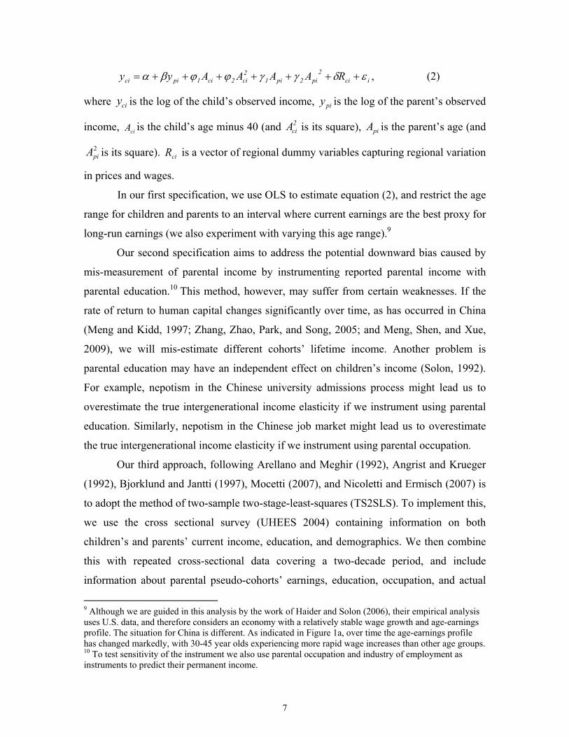
These samples are found to have a different age distribution, with both children
and parents being much younger in the parent-headed sample than in the child-headed
12 The UHIES is a nationwide survey (31 provinces) but due to confidentiality restrictions, we have access to data for only 16 provinces. There are 12 provinces included in the UHEES survey (Beijing, Shanxi, Liaoning, Heilongjiang, Zhejiang, Anhui, Hubei, Guangdong, Sichuan, Guizhou, Shaanxi, and Gansu). When using UHIES to estimate earnings equations as a base for predicted parental earnings, we use data for all 16 provinces we have access to (not just the 12 in the UHEES). 13 However, non-residing children of the household head and spouse are not surveyed. 14 For detailed description of the UHIES data, see Meng, Gong, and Wang, 2009.
9
sample (see Figure 3). We hope that combining the two samples will give us a sample of
parents and children who are reasonably representative of the general population.
The UHEES data includes 28,729 child-parent pairs. Excluding pairs with
children younger than 16 or currently at school, those with an intergenerational age
difference below 14 years, there are 18,596 child-parent pairs. We further restrict our
sample to those who are working and who have a positive income in 2004 with a father
or mother who is no older than 74 and 69 in 2004, respectively.15 With these further
restrictions and excluding missing values and very few outliers 5475 child-father and
3431 child-mother pairs remain in the sample.16 For some of our specifications, we
restrict the sample to those where both the parent and child are within the working-age
range and are currently (in 2004) working, and with non-missing income data. This
further reduces the sample size to 1813.17
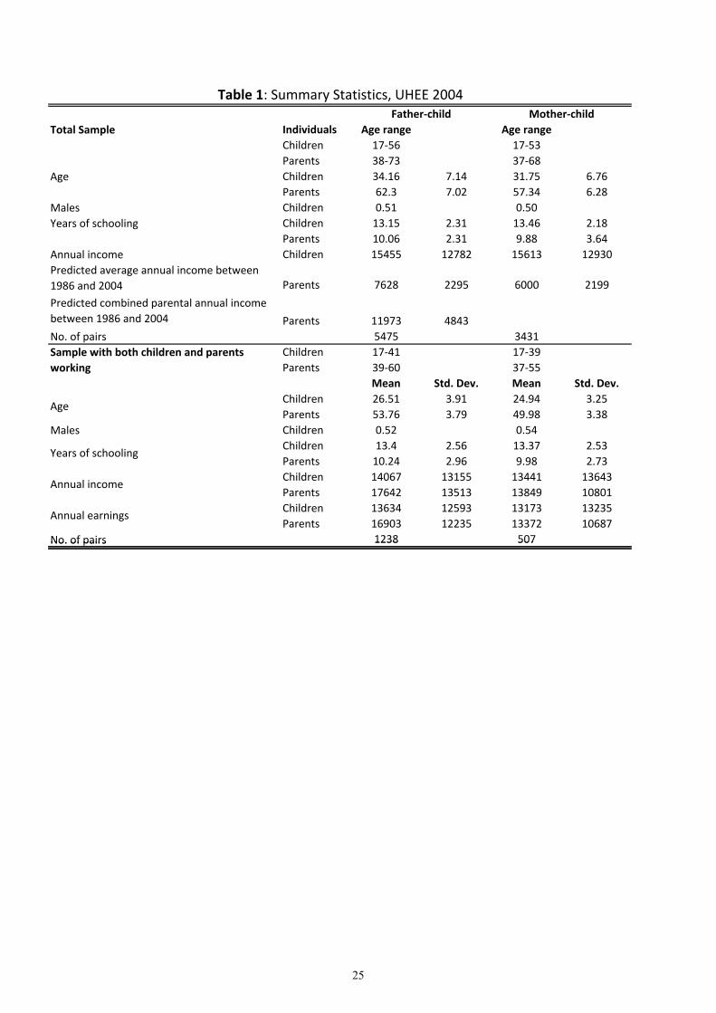
The summary statistics of children’s and parents’ ages, years of education, income,
and earnings are reported in Table 1.18 The top panel reports all child-parent pairs in our
UHEES sample, while the lower panel reports the sample in which both children and
parents are working in 2004. Below we only discuss in detail the bottom panel results.
Children are between 17 and 41 years old, fathers between 39 and 60 and mothers
between 37 and 55. The average age is about 26 for children, 54 for fathers and 50 for
mothers. Slightly more than half of the sample children are males. The average number of
years of schooling is about 13.5 for children and 10 for parents. The table also shows that
(conditional on working) fathers have the highest income and earnings on average,
followed by children and then mothers.
15 This is because when using UHIES data to predict for parental earnings, we restrict for each year that father's and mother's age should be no older than 60 and 55, respectively, they should have at least 5 years of predicted earnings to be included in the sample. The earliest data we have for UHIES is 1986 and to have at least 5 years of predicted earnings the parents have to be no older than 60 or 55 in 1990 (no older than 74 and 69 in 2004). 16 This is the sample used in Table 3A. Summing across the four combinations (father-son, father-daughter, mother-son, mother-daughter), the sample size is 2813+2662+1734+1697=8906. 17 This is the sample used in Table 2. Summing across the four combinations (father-son, father-daughter mother-son, , mother-daughter), the sample size is 646+313+592+262=1813. 18 The incomes in this study are in 2004 prices, based on provincial urban CPI indices.
10
4. Estimated Intergenerational Income Elasticity
The intergenerational income elasticity is estimated using Equation (2) for father-
son, father-daughter, mother-son and mother-daughter and for the different age groups of
children separately. We use the three different methods discussed in Section 2. The
results from the first method (OLS using just the 2004 UHEES) are presented in the top
panel of Table 2. Controlling for child and parent age and their square terms, we estimate
a father-son income elasticity of 0.24. Restricting children’s age to above 23 and further
to above 30, the elasticities increase to 0.25 and 0.32, respectively. A similar pattern is
found for father-daughter, mother-son, and mother-daughter elasticities. However, when
we restrict the sample to children aged 30 and above, we have relatively few observations
with which to estimate mother-son and mother-daughter elasticities and the resulting
income elasticities are not precisely estimated. In general, the parent-son elasticities are
higher than the parent-daughter elasticities. For the sample of all children, the R-squared
statistics range between 0.25 and 0.35, suggesting that parental income and the other
demographic controls in our regression can explain up to one-third of the variation in
children’s incomes. (Note that we do not report the R-squared in subsequent
specifications, since it is not a particularly meaningful statistic in instrumental variable
regressions.)
The bottom panel of Table 2 presents the results using one cross-sectional survey
(the 2004 UHEES), but instrumenting income using parental demographics. The
estimated elasticities increase somewhat, but the general pattern does not change much.
Again, given that the sample size in the mother-son and mother-daughter samples is
extremely small, so we do not place much weight on these estimated intergenerational
elasticities.
We then move to use predicted parental income from the UHIES data to estimate
Equation (2). Before we do so, we report some basic statistics of the predictions of the
parental permanent income and examine briefly the relationship between predicted
parental permanent income and their observed income in 2004 for a sample of parents
who are working in 2004 and have reported a positive income.
11
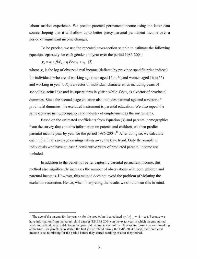
On average fathers’ permanent incomes are predicted using 13 years of data,
while mothers’ permanent incomes are predicted using 12 years of past income data.
Figure 4 shows the distribution of the number of years’ income used in this analysis.
Only 5 per cent of the sample have 5 or fewer years of data, while many have 10 years or
more. These data should give us a fairly good measure of the permanent income. As
indicated in Mazumder (2005) more years of data eliminates the downward bias due to
persistent transitory shocks and corrects for the age-related errors-in-variables bias. In
addition, as discussed in Section 2 there have been significant changes in the earnings
levels and earnings determination mechanism. Using average predicted earnings from
repeated cross-sectional data for the past 20 years will help us account for the non-linear
impact of these changes in earnings, thereby helping to reduce errors-in-variables bias.
We then examine the relationship between parental predicted permanent incomes
and their reported income in 2004 for a group of parents who were working in 2004 and
had positive income. Figure 5 shows a strong positive relationship between current and
predicted permanent income (the correlation coefficient is 0.46 for fathers and 0.55 for
mothers). In Figure 6, we plot the difference between the current income and predicted
permanent income for both mothers and fathers and find only a modest difference
between their current and permanent incomes. For both fathers and mothers, the standard
deviation of the difference is about 0.6, suggesting that for two-thirds of respondents, the
difference between their permanent and current incomes is less than 60 log points (about
80 percent). This is a larger gap than one would expect to observe in a developed nation,
but as we have noted, the rapid changes in the Chinese labor market over recent decades
have had quite differential impacts across the working-age population.
Having examined the reliability of the predicted permanent income data for
parents, we use these data to estimate Equation (2) and report the results in Table 3.
Columns 1 to 4 in panels A and B of Table 3 show father-child and mother-child
intergenerational income elasticities for different age groups of children, while column 5
restricts the sample to individuals whose fathers were working in 2004. Thus, the
permanent income elasticities reported in column 5 are essentially comparable to the
12
current income elasticities reported in columns 1 and 4 of Table 2 (which use current year
reported incomes for both children and parents).19
The father-son income elasticities estimated using predicted permanent fathers’
incomes are more than double those estimated using current year reported income. For
example, for the group of sons aged 30-42 in 2004 the estimated intergenerational income
elasticity is 0.32 using reported father’s income for 2004 (Table 2, Panel A, column 3,
first row). Instrumenting father’s income, the elasticity is 0.23 (Table 2, Panel B, column
3). However, if we use fathers’ permanent income – instrumented with education – the
intergenerational elasticity rises to 0.74 (Table 3, Panel A, column 4).20 A similar pattern
is found if the sample is restricted to cases in which the father worked in 2004. In this
sample, the elasticity using reported father income in 2004 is 0.24 (column 1 of Table 2),
while using father’s predicted permanent income the elasticity increases to 0.45 (column
5 in Panel A of Table 3).
For father-daughter pairs, the increase in elasticity when using fathers’ permanent
income relative to using fathers’ reported income is almost the same as for the father-son
pairs. For mother-son and mother-daughter pairs, the increase in estimated elasticities
from using mothers' permanent income is not as large as for father-son and father-
daughter pairs, but the general pattern is consistent.
Our preferred specification restricts the sample to children aged 30-42 (to account
for lifecycle bias), and uses parental predicted permanent income. The estimated
elasticities in this specification are 0.74 for father-son, 0.84 for father-daughter, 0.33 for
mother-son, and 0.47 for mother-daughter.
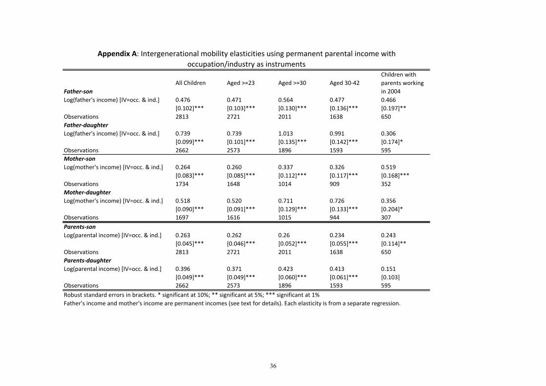
The above results use predicted parental permanent income with education as the
instrument. We also estimated the same regressions using predicted parental permanent
income with occupation and industry as the instruments. The results are presented in
19 The sample sizes in columns 1 and 4 of Table 2 are slightly smaller than those shown in column 5 of Table 3A, since there are a handful of parents who are working but for whom we do not observe incomes. Dropping these cases makes no substantive difference to the comparison – the elasticity is much higher when we use permanent parental incomes (Table 3A) than when we use one-year parental incomes (Table 2). 20 In practice, the age range of the sample that uses current father’s income (Table 2, column 3, third row) is 30-39. However, if we place the same age restriction on the sample that uses permanent father’s income (Table 3A, column 4), we obtain results very similar to those reported in Table 3A .
13

Appendix A. Using occupation and industry as instruments the estimated
intergenerational elasticities are lower than using education (but still much higher than
those using current parental income). In attempting to see what explains the difference,
we found that the unconditional correlation between child income and parental income is
very similar using either instrument set (see Appendix B for the comparison of the
unconditional relationships). Only when we introduce regional dummy variables into the
regression do the estimates diverge. Our conjecture is that perhaps within a particular
region there is more income variation across education levels than across
occupation/industry groups. Thus, within a particular region the predicted income using
education has more variation than predicted income using occupation and industry.
We also estimated the elasticity of children’s incomes with respect to their
parents’ combined incomes. The results are presented in Panel C of Table 3. In this
specification, the sample is restricted to children whose father works (and thus the sample
size is the same as for the father estimates in Table 3A). Note that in the case of two-
earner households, combined parental income is the sum of both parents’ incomes and in
the case of one-earner households, just the father’s income. The parent-son elasticity is
0.55 for sons at all ages, and increases slightly to 0.59 when we restrict the sample to
sons aged 30-42. This estimate lies below the corresponding father-son elasticities and
above mother-son elasticities estimates reported in Panel A and Panel B, respectively.
Our estimated parent-son elasticities are closer to the father-son estimates than to the
mother-son estimates. This is simply an indication that by definition fathers’ incomes
dominate the measure of combined parental income.
Our findings are quite consistent with the literature, which shows that the longer
the period used to generate parental permanent income, the lower is the attenuation bias
and the larger the estimated intergenerational income elasticity. For example, Mazumder
(2005) finds that using two year average data for the US the estimated IGE is 0.25 for
father-son pairs. It rises to 0.61 when using 16 years’ of father’s earnings, an increase of
144 per cent. Mazumder (2005) attributes the higher estimate to reducing the downward
bias that stems from transitory shocks and correcting for age-related errors-in-variables
bias.
14
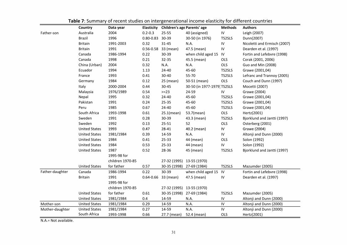
Cross-country comparison of intergenerational income mobility is hampered by
the fact that different studies use a variety of empirical methods, and observe children at
different ages. The intergenerational income elasticity for father-son is the most
commonly estimated in the literature. Table 7 compares our results with some recent
estimates of intergenerational elasticities (most are for fathers and sons, but some are
estimated for other family combinations).
Comparing our TS2SLS results for son aged 30 to 42 with the studies that use
similar methods and restrict children to those aged in their thirties and forties, we find
that our estimated father-son intergenerational income elasticity in urban China (0.74) is
at the upper end of the range of estimates for other countries. For example, the estimated
elasticity is 0.22 for Canada (Fortin and Lefebvre, 1998), about 0.25 for Australia (Leigh,
2007), 0.28 for Sweden (Bjorklund and Jantti, 1997), 0.41 for France (leFranc and
Trannoy, 2005), 0.44 for Italy (Mocetti, 2007), and 0.4−0.6 for the United States (Solon,
1992; Mazumder, 2005).21
5. How Is Income Earning Ability Transmitted Across Generations?
In this section, we analyze how income earning ability is transferred across
generations in urban China, focusing particularly on the role of education, party
membership, occupation and industry.
Education is believed to be a significant pathway of intergenerational
transmission for many countries. 22 Using our full sample, we therefore estimate
intergenerational educational transmission by both schooling years and by categories of
educational attainment: (1) lower secondary schooling or less; (2) upper secondary
schooling; (3) college and above.
21 There are too few studies of father-daughter, mother-son, and mother-daughter elasticities to draw strong conclusions about how our results compare with those for other countries. However, given that these elasticities tend to be highly correlated within countries, it seems reasonable to conclude that urban China is relatively socially immobile for women as well as men. 22 For instance, when education is not subsidized, rich parents can invest more in their children’s education than poor parents. Subsidized education can be a way of equalizing opportunities for poor children (Eide and Showalter, 1999; Ng, 2007).
15
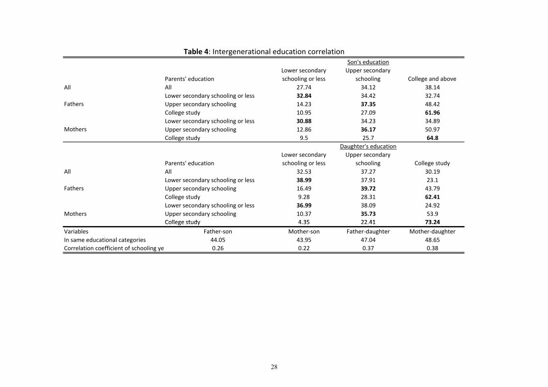
Table 4 cross tabulates the education level of parents and children. In the total
sample, 28 percent of sons have lower secondary schooling or less, 34 percent have upper
secondary schooling, and 38 percent have a college degree. Depending on which
combination we look at (father-son, father-daughter, mother-son, or mother-daughter),
between 44 and 49 percent of children are in the same education category as their parents.
Measured in years of schooling rather than categorically, the correlation coefficient
between parents’ and children’s education ranges from 0.22 for mothers and sons to 0.38
for mothers and daughters (see the bottom panel of Table 4). Among fathers who have a
college degree, 62 percent of their sons have a college degree. Among mothers with a
college degree, 65 percent of their sons have a college degree. A similar pattern can be
observed for daughters.
Figure 7 presents the estimated relationship between parents' and children's
schooling years by children’s birth year and gender, with the sample restricted to children
aged 25 years or older (since respondents aged less than 25 are more likely to be in the
process of completing their education). The chart shows that the intergenerational
association of schooling is approximately three times higher for children born in the late-
1970s than for children born in the early-1950s. This increase can be explained partly by
the end of the Chinese Cultural Revolution in 1976, followed by the restoration of the
University Entrance Examinations in 1977. For children born after 1960, this increased
the gap in educational attainment between those with higher-educated parents and those
with less-educated parents (Meng and Gregory, 2002).
By international standards, the intergenerational education correlation in urban
China is relatively low (compare our results with Hertz et al., 2007), although it has
increased significantly over the past half-century. The main factor in this is the high
persistence of college attainment across generations.
Parents’ social networks can play an important role in providing their children
with access to better opportunities in both education and the labor market (Lin and Bian,
1991; Walder, Li and Treiman, 2000; Meng, 2007). Communist Party membership can be
transferred across generations through parental role models and social networks. The
intergenerational transmission of occupations and industries is more complicated. It
16
depends on whether the parental social network plays an important role in children’s
entrance to the labor market and their promotion in the workplace; whether there are
entry barriers due to crafts, professional and technical skills that are handed down;
whether the attitudes and norms of family ties differ between rich and poor parents; and
whether cohabitation with parents strengthens intergenerational persistence through the
effects on beliefs and preferences (Mocetti, 2007).
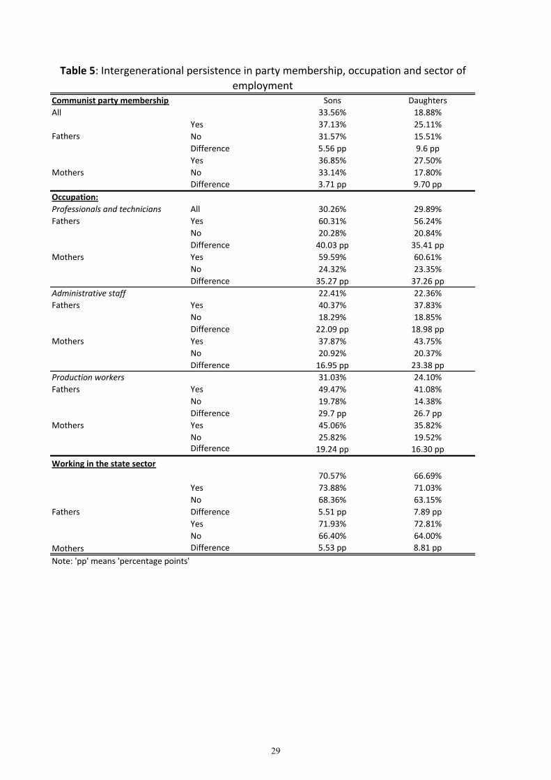
Table 5 reports the persistence matrices of Communist Party membership,
occupation, and sector of employment between children and parents by gender using the
total sample. The first panel of Table 5 shows that if the parents are party members, their
children are between 4 and 10 percentage points more likely to be party members (for
sons, this represents about a 10-20 percent increase in the probability of joining the party,
while for daughters it represents a more than 50 percent increase in the probability of
party membership). The second panel indicates a very strong persistence in occupation
between children and parents. If fathers or mothers are working in the occupation
“professionals and technicians”, their children are 35-40 percentage points more likely to
also be working in this occupation than those whose parents are not (this represents a
near-tripling in the probability of being in this occupational category). The differences for
“administration staff” are 17-23 percentage points (approximately a doubling in the
probability), while for “production and transportation workers” the differences are 16-30
percentage points (having a father who was a production worker approximately triples the
probability that a child will enter this occupational grouping, while having a mother who
was a production worker doubles the probability).
The third panel of Table 5 presents the proportions of sons and daughters working
in the state-owned sector based on whether their fathers and mothers also work in that
sector. Seventy-one percent of sons and 67 percent of daughters work in the state-owned
sector. Children are 6-9 percentage points (about 10 percent) more likely to work in the
state-owned sector if one of their parents also worked in that sector.
17
6. Conclusions
An old Chinese saying holds that families will “be poor no more than three
generations and be rich no more than three generations”.23 This suggests that in China, as
in many nations, there is a strong popular belief in social mobility. Our findings challenge
this view. At least for modern-day urban China, we find a strikingly low level of
intergenerational mobility. Our preferred estimates show that the intergenerational
income elasticities are 0.74 for father-son, 0.84 for father-daughter, 0.33 for mother-son,
and 0.47 for mother-daughter. Internationally, our estimated father-son elasticity places
urban China among the least socially mobile places in the world.
Empirically, our analysis shows the importance of obtaining a measure of
permanent income, and accounting for lifecycle bias. If we use single-year income
measures for parents, we obtain substantially lower estimates of the intergenerational
income elasticity for China (indeed, such estimates imply that urban China is an
extremely socially mobile place). However, when we use predicted permanent incomes,
and restrict the sample of children to those aged 30-42 (to account for lifecycle bias), we
obtain intergenerational elasticities that are sometimes twice as large.
Note that we do not formally calculate intergenerational correlations for urban
China, since doing so would require information on the underlying variance in permanent
incomes (recall that we predict parental income using parental demographics). However,
given that income inequality in urban China (measured by annual incomes) has risen
markedly over recent decades, it is likely that inequality of permanent incomes has also
risen. The intergenerational correlation (ρ) is simply equal to the elasticity (β), multiplied
by the ratio of the standard deviation of log income in the parents’ generation (σp) and the
children’s generation (σc), i.e. c
p
σσ
βρ = . Since permanent income is likely more
dispersed in the 2000s than in the 1980s, it is probable that the intergenerational income
correlation in urban China would be lower than the intergenerational income elasticity.24
23 “Qiong bu guo san dai, fu bu guo san dai”. 24 For example, the coefficient variation of annual real earnings rose from 0.45 in 1988 to 0.81 in 2004.
18
However, even taking this into account, China’s intergenerational correlation is likely to
be higher than that observed for most developed nations.
Another factor to bear in mind is that our study focuses only on urban China.
Given the large income differences between rural and urban China, it is likely that
intergenerational mobility is higher for individuals born in rural parts of the country, and
therefore that the intergenerational elasticity of income (or earnings) for the entire
country is likely to be lower than that which we estimate for urban China. However, from
a policy perspective, our estimated elasticity is still an important parameter. Although
rural-urban migration offers the potential for upwards social mobility for those born in
rural areas, it only offers the potential for downwards social mobility for those born in
urban areas.
Exploring possible pathways, we find that education, especially college study, is
one channel through which earnings ability is transmitted from parents to children
(though the intergenerational association of education is still lower in urban China than in
many other nations). We also find intergenerational correlations for parental party
membership, occupation, and industry. The occupational correlation is particularly high,
suggesting that occupation may be the most important channel through which
intergenerational transmission occurs in urban China. However, it is also possible that
factors we do not perfectly observe in our data – such as genes, health, or social networks
– are also significant explanators of intergenerational transmission in urban China.
19
References Altonji, Joseph G. and Dunn, Thomas A. (2000). “An Intergenerational Model of Wages,
Hours and Earnings.” The Journal of Human Resources, Vol. 35 (2), pp. 221-258.
Angrist, Joshua D. and Krueger, Alan B. (1992). “The effect of age at school entry on
educational attainment: an application of instrumental variables with moments
from two samples.” Journal of the American Statistical Association, Vol.
87 (418), pp. 328–336.
Arellano, M. and Meghir, C. (1992). “Female labour supply and on-the-job search: an
empirical model estimated using complementary data sets.” Review of Economic
Studies, Vol. 59 (3), 537–559.
Becker, Gary S. and Tomes, Nigel (1979). “An Equilibrium Theory of the Distribution of
Income and Intergenerational Mobility.” Journal of Political Economy, Vol. 87 (6),
pp. 1153-1189.
Benjamin, Dwayne; Brandt, Loren, Giles, John and Wang, Sangui (2005). “Income
Inequality During China’s Economic Transition.” Chapter 18, in Brandt, Loren and
Rawski, Thomas (ed.), China's Economic Transition: Origins, Mechanisms, and
Consequences.
Bian, Yanjie (2002). “Chinese Social Stratification and Social Mobility.” Annual Review
of Sociology, Vol. 28, pp. 91-116.
Bjorklund, Anders and Jantti, Markus (1997). “Intergenerational Income Mobility in
Sweden Compared to the United States.” American Economic Review, Vol. 87 (5),
pp. 1009-1018.
Bohlmark, Anders and Lindquist, Matthew J. (2006). “Life-cycle Variations in the
Association Between Current and Lifetime Income: Replication and Extension for
Sweden.” Journal of Labor Economics, Vol. 24 (4), pp. 878-896.
20

Cai, Fang; Giles, John and Meng, Xin (2006). “How Well do Children Insure Parents
Against Low Retirement Income? Evidence from Urban China.” Journal of Public
Economics, Vol. 90, pp. 2229-2255.
Chadwick, Hardy L. and Solon, Gary (2002). “Intergenerational Income Mobility
Among Daughters.” American Economic Review, Vol. 92 (1), pp. 335-344.
Cheng, Yuan and Dai, Jiangzhong (1995). “Intergenerational Mobility in Modern
China.” European Sociological Review, Vol. 11 (1), pp. 17-35.
Corak, Miles (2001). “Are the Kids All Right: Intergenerational Mobility and Child Well-
Being in Canada.” In Keith Banting, Andrew Sharpe and France St-Hilaire
(editors). Review of Economic Performance and Social Progress. Montreal and
Ottawa: Institute for Research on Public Policy and Centre for the Study of Living
Standards.
Corak, Miles (2006). “Do Poor Children Become Poor Adults? Lessons from a Cross
Country Comparison of Generational Earnings Mobility.” Research on Economic
Inequality, Vol. 13 (1), pp. 143-188.
Couch, Kenneth A. and Dunn, Thomas A. (1997). “Intergenerational Correlations in
Labor Market Status: A Comparison of the United States and Germany.” Journal of
Human Resources, Vol. 32 (1), pp. 210-232.
Dearden, Lorraine, Machin, Michael S. and Reed, Howard (1997). “Intergenerational
Mobility in Britain.” Economics Journal, Vol. 107 (1), pp. 47-66.
Dunn, Christopher, E. (2007). “The Intergenerational Transmission of Lifetime Earnings:
Evidence from Brazil.” The B.E. Journal of Economic Analysis & Policy, Vol. 7 (2)
(Contributions), Article 2.
Eide, Eric R. and Showalter, Mark H. (1999). “Factors Affecting the Transmission of
Earnings Across Generations: A Quantile Regression Approach.” The Journal of
Human Resources, Vol. 34 (2), pp. 253-267.
Ferreira, Sergio and Veloso, Fernando (2006). “Intergenerational Mobility of Wages in
Brazil.” Brazilian Review of Econometrics, Vol. 26 (2), pp. 181-211.
21
Fortin, Nicole M. and Lefebvre, Sophie (1998). “Intergenerational Income Mobility in
Canada.” In M. Corak (ed.) Labor Markets, Social Institutions, and the Future of
Canada’s Children, pp. 51-64. Statistics Canada, Ottawa.
Grawe, Nathan D. (2001). “Intergenerational Mobility in the U.S. and Abroad: Quintile
and Mean Regression Measures.” PhD. Dissertation, Department of Economics,
University of Chicago.
Grawe, Nathan D. (2004). “Intergenerational Mobility for Whom? The Experience of
High- and Low- Earnings Sons in International Perspective.” In Miles Corak (ed.),
Generational Income Mobility in North America and Europe. Cambridge:
Cambridge University Press.
Grawe, Nathan. D. (2006). “Life Cycle Bias in the Estimation of Intergenerational
Earnings Persistence.” Labor Economics, Vol. 13 (5), pp. 551-570.
Guo, Congbin and Min, Weifang (2008). “Education and Intergenerational Income
Mobility in Urban China.” Front Education China, Vol. 3 (1), pp. 22-24.
Translated from: Educational Research (Jiaoyu Yanjiu), Vol (5), pp. 3–14.
Haider, Steven and Solon, Gary (2006). “Life-cycle Variation in the Association
Between Current and Lifetime Earnings.” American Economic Review, Vol. 96 (4),
pp. 1308-1320.
Hertz, Thomas (2001). “Education, Inequality and Economic Mobility in South Africa.”
PhD Dissertation, University of Massachusetts, U.S.
Hertz, Tom, Jayasundera, Tamara, Piraino, Patrizio, Selcuk, Sibel, Smith, Nicole and
Verashchagina, Alina (2007). “The Inheritance of Educational Inequality:
International Comparisons and Fifty-Year Trends.” The B.E. Journal of Economic
Analysis & Policy, Vol. 7 (2) (Advances), Article 10.
Lee, Chul-In and Solon, Gary (2006). “Trends in Intergenerational Income Mobility.”
NBER Working Paper, No. 12007, Cambridge, MA: National Bureau of Economic
Research.
22
Lefranc, Arnaud and Trannoy, Alain (2005). “Intergenerational Earnings Mobility in
France: Is France More Mobile than the U.S.?” Annales d’Economie et de
Statistique, Vol. 78, pp. 57-78.
Leigh, Andrew (2007). “Intergenerational Mobility in Australia.” The B.E. Journal of
Economic Analysis & Policy: Vol. 7 (2) (Contributions), Article 6.
Lin, Nan and Bian, Yanjie (1991). “Getting Ahead in Urban China.” The American
Journal of Sociology, Vol. 97 (3), pp. 657-688.
Mazumder, Bhashkar (2005). “Fortunate Sons: New Estimates of Intergenerational
Mobility in the United States Using Social Security Earnings Data.” Review of
Economics and Statistics, Vol. 87 (2), pp. 235-255.
Meng, Xinand Kidd, Michael (1997). “Wage Determination in China’s State Sector in
the 1980s”, Journal of Comparative Economics, 25 (3), pp. 403-421.
Meng, Xin, Gong, Xiaodong, and Wang, Youjuan (2009). “Impact of Income Growth
and Economic Reform on nutrition intake in urban China: 1986-2000”,
Economic Development
and Cultural Change, 57 (2), pp. 261-295.
Meng, Xin and Gregory, Robert G., (2002). “The Impact of Interrupted Education on
Subsequent Educational Attainment: a Cost of the Chinese Cultural Revolution.”
Economic Development and Cultural Change, Vol. 50 (4), pp. 935-959.
Meng, Xin (2004). “Economic Restructuring and Income Inequality in Urban China.”
Review of Income and Wealth, Vol. 50 (3), pp. 357-379.
Meng, Xin (2007). "Wealth Accumulation and Distribution in Urban China." Economic
Development and Cultural Change, Vol. 55 (4), pp. 761-791.
Mocetti, Sauro (2007). “Intergenerational Earnings Mobility in Italy.” The B.E. Journal of
Economic Analysis & Policy, Vol. 7 (2) (Contributions), Article 5.
Nicoletti, Cheti and Ermisch John F. (2007). “Intergenerational Earnings Mobility:
Changes Across Cohorts in Britain.” The B.E. Journal of Economic Analysis &
Policy: Vol. 7 (2) (Contributions), Article 9.
23
Osterbacka, Eva (2001). “Family Background and Economic Status in Finland.”
Scandinavian Journal of Economics, Vol. 103 (3), pp. 467-484.
Solon, Gary (1992). “Intergenerational Income Mobility in the United States.” American
Economic Review, Vol. 82 (3), pp. 293-408.
Takenoshita, Hirohisa (2007). “Intergenerational Mobility in East Asian Countries: A
Comparative Study of Japan, Korea and China.” International Journal of Japanese
Sociology, Vol. 16 (1), pp. 64-79.
Walder, Andrew G. Li, Bobai and Treiman, Donald J. (2000). “Politics and Life
Chances in a State Socialist Regime: Dual Career Paths into Urban Chinese Elite,
1949-1996.” American Sociological Review, Vol. 65 (2), pp. 191-209.
Wu, Xiaogang and Treiman, Donald J. (2003). “The Household Registration System and
Social Stratification in China: 1955-1996.” California Center for Population
Research On-Line Working Paper, No. CCPR-006-03.
Yu, Hong and Liu, Xin (2004). “Did the Effect of Work Unit on Intergenerational
Mobility in Urban China Decline?” Sociology Studies (in Chinese), Vol. 114
Zhang, Junsen, Zhao, Yaohui, Park, Albert, and Song, Xiaoqing (2005). “Economic
returns to schooling in urban China, 1988-2001”, Journal of Comparative
Economics, Vol. 33, pp. 730-752.
24
No. of 1238 507
Table 1: Summary Statistics, UHEE 2004Father‐child Mother‐child
Total Sample Individuals Age range Age rangeChildren 17‐56 17‐53Parents 38‐73 37‐68
Age Children 34.16 7.14 31.75 6.76Parents 62.3 7.02 57.34 6.28
Males Children 0.51 0.50Years of schooling Children 13.15 2.31 13.46 2.18
Parents 10.06 2.31 9.88 3.64Annual income Children 15455 12782 15613 12930Predicted average annual income between 1986 and 2004 Parents 7628 2295 6000 2199
Predicted combined parental annual income between 1986 and 2004 Parents 11973 4843No. of pairs 5475 3431Sample with both children and parents working
Children 17‐41 17‐39Parents 39‐60 37‐55
Mean Std. Dev. Mean Std. Dev.
AgeChildren 26.51 3.91 24.94 3.25Parents 53.76 3.79 49.98 3.38
Males Children 0.52 0.54
Years of schoolingChildren 13.4 2.56 13.37 2.53Parents 10.24 2.96 9.98 2.73
Annual incomeChildren 14067 13155 13441 13643Parents 17642 13513 13849 10801
Annual earningsChildren 13634 12593 13173 13235Parents 16903 12235 13372 10687
No. of pairspairs 1238 507
25
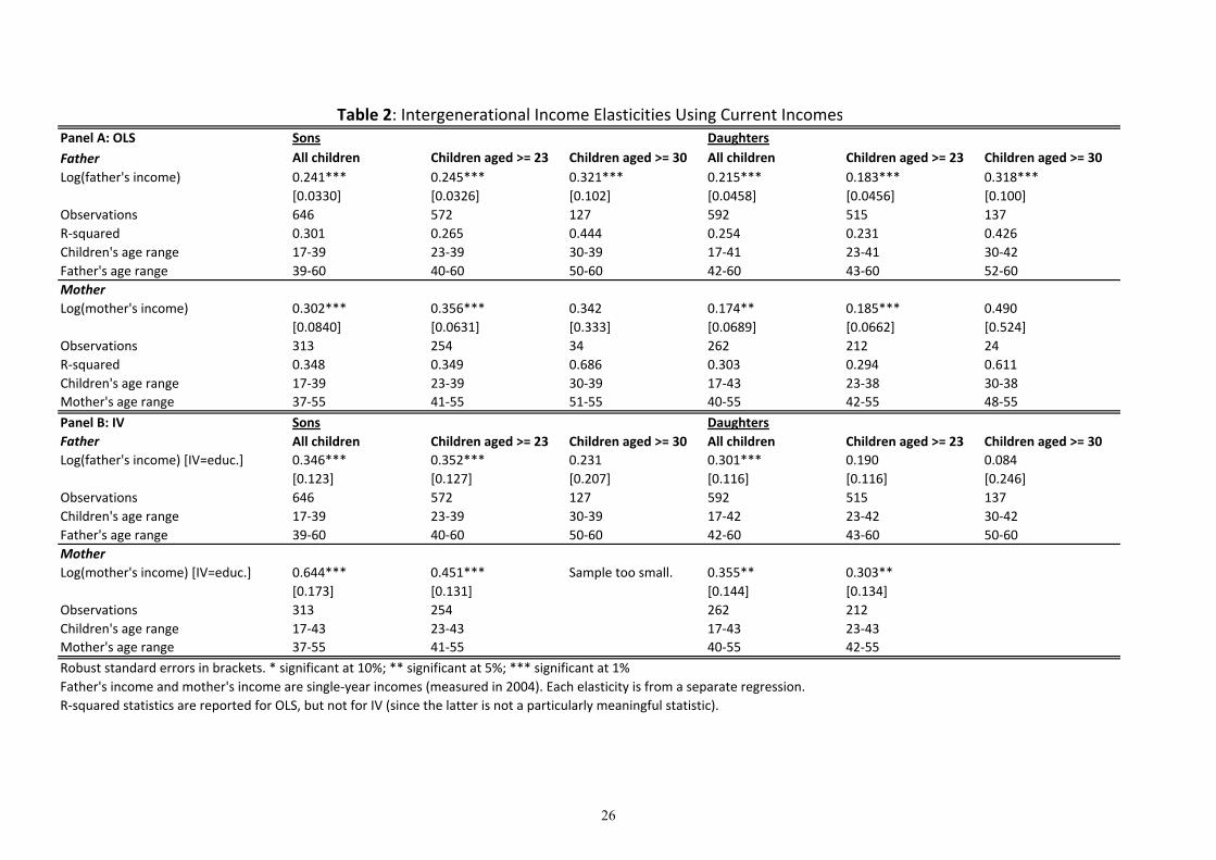
Table 2: Intergenerational Income Elasticities Using Current IncomesPanel A: OLS Sons Daughters
Father All children Children aged >= 23 Children aged >= 30 All children Children aged >= 23 Children aged >= 30Log(father's income) 0.241*** 0.245*** 0.321*** 0.215*** 0.183*** 0.318***
[0.0330] [0.0326] [0.102] [0.0458] [0.0456] [0.100]Observations 646 572 127 592 515 137R‐squared 0.301 0.265 0.444 0.254 0.231 0.426Children's age range 17‐39 23‐39 30‐39 17‐41 23‐41 30‐42Father's age range 39‐60 40‐60 50‐60 42‐60 43‐60 52‐60MotherLog(mother's income) 0.302*** 0.356*** 0.342 0.174** 0.185*** 0.490
[0.0840] [0.0631] [0.333] [0.0689] [0.0662] [0.524]Observations 313 254 34 262 212 24R‐squared 0.348 0.349 0.686 0.303 0.294 0.611Children's age range 17‐39 23‐39 30‐39 17‐43 23‐38 30‐38Mother's age range 37‐55 41‐55 51‐55 40‐55 42‐55 48‐55
Panel B: IV Sons DaughtersFather All children Children aged >= 23 Children aged >= 30 All children Children aged >= 23 Children aged >= 30Log(father's income) [IV=educ.] 0.346*** 0.352*** 0.231 0.301*** 0.190 0.084
[0.123] [0.127] [0.207] [0.116] [0.116] [0.246]bObservations 646 572 127 592 515 137
Children's age range 17‐39 23‐39 30‐39 17‐42 23‐42 30‐42Father's age range 39‐60 40‐60 50‐60 42‐60 43‐60 50‐60MotherLog(mother's income) [IV=educ.] 0.644*** 0.451*** Sample too small. 0.355** 0.303**
[0.173] [0.131] [0.144] [0.134]Observations 313 254 262 212Children's age range 17‐43 23‐43 17‐43 23‐43Mother's age range 37‐55 41‐55 40‐55 42‐55
Robust standard errors in brackets. * significant at 10%; ** significant at 5%; *** significant at 1%Father's income and mother's income are single‐year incomes (measured in 2004). Each elasticity is from a separate regression. R‐squared statistics are reported for OLS, but not for IV (since the latter is not a particularly meaningful statistic).
26
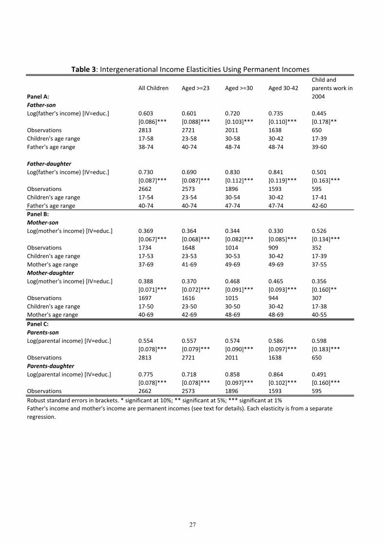
Table 3: Intergenerational Income Elasticities Using Permanent Incomes
Panel A: All Children Aged >=23 Aged >=30 Aged 30‐42
Child and parents work in 2004
Father‐sonLog(father's income) [IV=educ.] 0.603 0.601 0.720 0.735 0.445
[0.086]*** [0.088]*** [0.103]*** [0.110]*** [0.178]**Observations 2813 2721 2011 1638 650Children's age range 17‐58 23‐58 30‐58 30‐42 17‐39Father's age range 38‐74 40‐74 48‐74 48‐74 39‐60
Father‐daughterLog(father's income) [IV=educ.] 0.730 0.690 0.830 0.841 0.501
[0.087]*** [0.087]*** [0.112]*** [0.119]*** [0.163]***Observations 2662 2573 1896 1593 595Children's age range 17‐54 23‐54 30‐54 30‐42 17‐41Father's age range 40‐74 40‐74 47‐74 47‐74 42‐60Panel B:Mother‐sonLog(mother's income) [IV=educ.] 0.369 0.364 0.344 0.330 0.526
[0.067]*** [0.068]*** [0.082]*** [0.085]*** [0.134]***Observations 1734 1648 1014 909 352Children's age range 17‐53 23‐53 30‐53 30‐42 17‐39Mother's age range 37‐69 41‐69 49‐69 49‐69 37‐55Mother‐daughterLog(mother's income) [IV=educ.] 0.388 0.370 0.468 0.465 0.356
[0.071]*** [0.072]*** [0.091]*** [0.093]*** [0.160]**Observations 1697 1616 1015 944 307Children's age range 17‐50 23‐50 30‐50 30‐42 17‐38Mother's age range 40‐69 42‐69 48‐69 48‐69 40‐55
Panel C:Parents‐sonLog(parental income) [IV=educ.] 0.554 0.557 0.574 0.586 0.598
[0.078]*** [0.079]*** [0.090]*** [0.097]*** [0.183]***Observations 2813 2721 2011 1638 650Parents‐daughterLog(parental income) [IV=educ.] 0.775 0.718 0.858 0.864 0.491
[0.078]*** [0.078]*** [0.097]*** [0.102]*** [0.160]***Observations 2662 2573 1896 1593 595
Robust standard errors in brackets. * significant at 10%; ** significant at 5%; *** significant at 1%Father's income and mother's income are permanent incomes (see text for details). Each elasticity is from a separate regression.
27
Lower schooling less
All 27.74 secondary schooling less 32.84 secondary schooling 14.23 study 10.95
Table education correlation
llege y 22 41 73 24
above
study
daughter
and 38.1432.7448.4261.96
34.8950.9764.8
.1923.143.7962.4124.9253.9
24.
48.650.38
College30
73
‐
College
Mother
secondary schooling34.1234.4237.3527.09
education
education
secondary
daughter
34.2336.1725.7
schooling37.2737.9139.7228.3138.0935.7322 41.
‐47.040.37
Upper
Upper
Son's
Daughter's
Father
less
secondary or
secondary or
535
‐son
30.8812.869.5
ling32.5338.9916.499.2836.9910.374 34.
Mother43.950.22
Lowerhoosc
less
less
ss
or
Intergenerational
or
or
or le
ing
schoolingschooling
schoolingschooling
oolschooling
‐son
:
n
sch
Father44.050.26
4
education
atio
secondarysecondarystudy
duc
secondarysecondarystudysecondarysecondarystudyud
ts' e
st
LowerUpperCollege
Parents'
LowerUpperCollege
ren
LowerUpperCollegeLowerUpperCollege
PaAll
Co
e yschoolingcategories
of
coefficient
Fathers
educational
Mothers
Fathers
Mothers
Variablessame
Correlation
All
All
In
28
Communist party
Occupation:Professionals and Fathers
Table 5:
All
Fathers
Mothers
pp pp
Difference pp
Difference pp
means 'percentage
Mothers
AdministrativeFathers
Mothers
Production Fathers
Mothers
Working in
Note: 'pp'
Fathers
Mothers
the state
workers
staff
sector
membership
technicians
Intergenerational
YesNo
points'
YesNo
N
N
Yes
Yes
YesNo
YesNo
No
YesNo
YesNo
AllYesNo
Yes
oDifference
oDifference
Difference
Difference
Difference
Difference
Difference
Difference
persistence in employment
party
5.5171.93%66.40%5.53
70.573.88%68.36%
25.819.24
19.729.745.06%
31.03%49.47%
37.87%20.92%16.95
40.37%18.29%22.09
24.32%35.2722.41%
Sons33.56%37.13%31.57%5.5636.85%33.14%3.71
30.26%60.31%20.28%40.0359.59%
membership,
7%
2% pp
8% pp
pp
pp
pp
pp
pp
pp
occupation
Daughters18.88%25.11%15.51%9.6 pp27.50%17.80%9.70 pp
29.89%56.24%20.84%35.41 pp60.61%23.35%37.26 pp22.36%37.83%18.85%18.98 pp43.75%20.37%23.38 pp24.10%41.08%14.38%26.7 pp
and sector
35.82%19.52%16.30 pp
66.69%71.03%63.15%7.89 pp72.81%64.00%8.81 pp
of
29
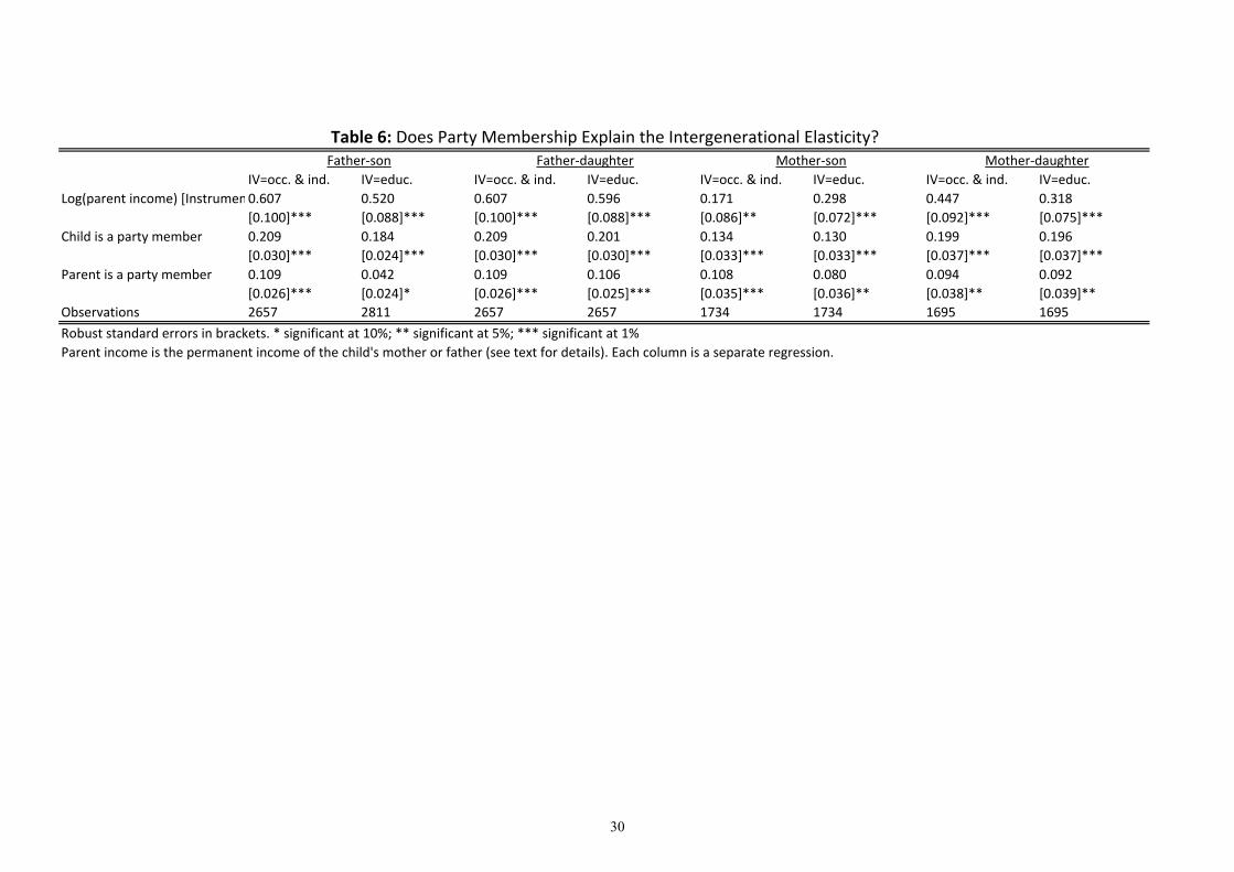
Table 6: Does Party Membership Explain the Intergenerational Elasticity?
Log(parent income)
Child is a party mem
Parent is a party me
Father‐son Father‐daughter Mother‐son Mother‐daughterIV=occ. & ind. IV=educ. IV=occ. & ind. IV=educ. IV=occ. & ind. IV=educ. IV=occ. & ind. IV=educ.
[Instrumen0.607 0.520 0.607 0.596 0.171 0.298 0.447 0.318[0.100]*** [0.088]*** [0.100]*** [0.088]*** [0.086]** [0.072]*** [0.092]*** [0.075]***
ber 0.209 0.184 0.209 0.201 0.134 0.130 0.199 0.196[0.030]*** [0.024]*** [0.030]*** [0.030]*** [0.033]*** [0.033]*** [0.037]*** [0.037]***
mber 0.109 0.042 0.109 0.106 0.108 0.080 0.094 0.092[0.026]*** [0.024]* [0.026]*** [0.025]*** [0.035]*** [0.036]** [0.038]** [0.039]**
Observations
Robust standard err
2657 2811 2657 2657 1734 1734 1695 1695
ors in brackets. * significant at 10%; ** significant at 5%; *** significant at 1%Parent income is the permanent income of the child's mother or father (see text for details). Each column is a separate regression.
30
Country Data year Elasticity Children's ageParents' age Methods AuthorsAustralia 2004 0.2‐0.3 25‐55 40 (assigned) IV Leigh (2007)Brazil 1996 0.80‐0.83 30‐39 30‐50 (in 1976) TS2SLS Dunn(2007)Britain 1991‐2003 0.32 31‐45 N.A. IV Nicoletti and Ermisch (2007)Britain 1991 0.56‐0.58 33 (mean) 47.5 (mean) IV Dearden et al. (1997)Canada 1986‐1994 0.22 30‐39 when child aged 15 IV Fortin and Lefebvre (1998)Canada 1998 0.21 32‐35 45.5 (mean) OLS Corak (2001, 2006)China (Urban) 2004 0.32 N.A. N.A. OLS Guo and Min (2008)Ecuador 1994 1.13 24‐40 45‐60 TS2SLS Grawe (2001,04)France 1993 0.41 30‐40 55‐70 TS2SLS Lefranc and Trannoy (2005)Germany 1984 0.12 25 (mean) 50‐51 (mean) OLS Couch and Dunn (1997)Italy 2000‐2004 0.44 30‐45 30‐50 (in 1977‐1979)TS2SLS Mocetti (2007)Malaysia 1976/1989 0.54 >=23 24‐59 IV Grawe (2004)Nepal 1995 0.32 24‐40 45‐60 TS2SLS Grawe (2001,04)Pakistan 1991 0.24 25‐35 45‐60 TS2SLS Grawe (2001,04)Peru 1985 0.67 24‐40 45‐60 TS2SLS Grawe (2001,04)South Africa 1993‐1998 0.61 25.1(mean) 53.7(mean) OLS Hertz(2001)Sweden 1991 0.28 30‐39 43.3 (mean) TS2SLS Bjorklund and Jantti (1997)Sweden 1992 0.13 25‐51 52 OLS Osterberg (2001)United States 1993 0 47 28 41 40 2 (mean) IV Grawe (2004)
Table 7: Summary of recent studies on intergenerational income elasticity for different countries
Father‐son
United States 1993 0.47 28‐41 40.2 (mean) IV Grawe (2004)United States 1981/1984 0.39 14‐59 N.A. IV Altonji and Dunn (2000)United States 1984 0.41 25‐33 44 (mean) OLS Solon (1992)United States 1984 0.53 25‐33 44 (mean) IV Solon (1992)United States 1987 0.52 28‐36 45 (mean) TS2SLS Bjorklund and Jantti (1997)
United States
1995‐98 for children 1970‐85 for father 0.57
27‐32 (1995) 30‐35 (1998)
13‐55 (1970) 27‐69 (1984) TS2SLS Mazumder (2005)
Canada 1986‐1994 0.22 30‐39 when child aged 15 IV Fortin and Lefebvre (1998)Britain 1991 0.64‐0.66 33 (mean) 47.5 (mean) IV Dearden et al. (1997)
United States
1995‐98 for children 1970‐85 for father 0.61
27‐32 (1995) 30‐35 (1998)
13‐55 (1970) 27‐69 (1984) TS2SLS Mazumder (2005)
United States 1981/1984 0.4 14‐59 N.A. IV Altonji and Dunn (2000)Mother‐son United States 1981/1984 0.29 14‐59 N.A. IV Altonji and Dunn (2000)
United States 1981/1984 0.27 14‐59 N.A. IV Altonji and Dunn (2000)South Africa 1993‐1998 0.66 27.7 (mean) 52.4 (mean) OLS Hertz(2001)
N.A.= Not available.
Father‐daughter
Mother‐daughter
31
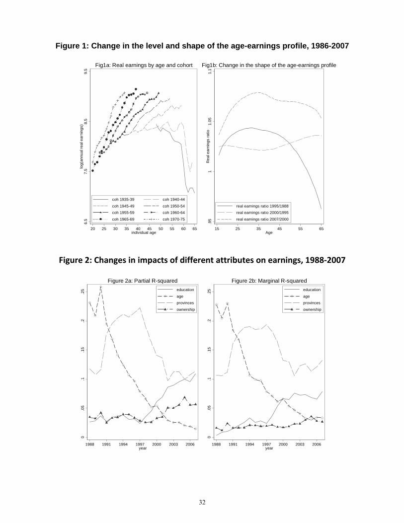
Figure 1: Change in the level and shape of the age-earnings profile, 1986-2007
6.5
7.5
8.5
9.5
log(
annu
al re
al e
arni
ngs)
20 25 30 35 40 45 50 55 60 65individual age
coh 1935-39 coh 1940-44
coh 1945-49 coh 1950-54coh 1955-59 coh 1960-64
coh 1965-69 coh 1970-75
Fig1a: Real earnings by age and cohort
.95
11.
051.
1R
eal e
arni
ngs
ratio
15 25 35 45 55 65Age
real earnings ratio 1995/1988real earnings ratio 2000/1995
real earnings ratio 2007/2000
Fig1b: Change in the shape of the age-earnings profile
Figure 2: Changes in impacts of different attributes on earnings, 1988‐2007
0.0
5.1
.15
.2.2
5
1988 1991 1994 1997 2000 2003 2006year
education
ageprovinces
ownership
Figure 2a: Partial R-squared
0.0
5.1
.15
.2.2
5
1988 1991 1994 1997 2000 2003 2006year
education
ageprovinces
ownership
Figure 2b: Marginal R-squared
32
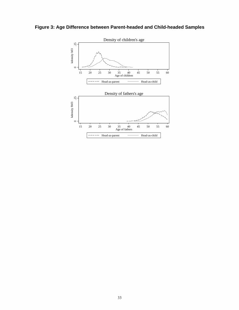
Figure 3: Age Difference between Parent-headed and Child-headed Samples
0.2
5kd
ensi
ty b
0315 20 25 30 35 40 45 50 55 60
Age of children
Head-as-parent Head-as-child
Density of children's age
0.2
5kd
ensi
ty fb
03
15 20 25 30 35 40 45 50 55 60Age of fathers
Head-as-parent Head-as-child
Density of fathers's age
33
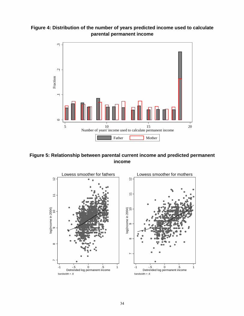
Figure 4: Distribution of the number of years predicted income used to calculate parental permanent income
0.1
.2.3
Frac
tion
5 10 15 20Number of years' income used to calculate permanent income
Father Mother
Figure 5: Relationship between parental current income and predicted permanent income
78
910
1112
log(
inco
me
in 2
004)
-1 -.5 0 .5 1Detrended log permanent income
bandwidth = .8
Lowess smoother for fathers
78
910
1112
log(
inco
me
in 2
004)
-1 -.5 0 .5 1Detrended log permanent income
bandwidth = .8
Lowess smoother for mothers
34
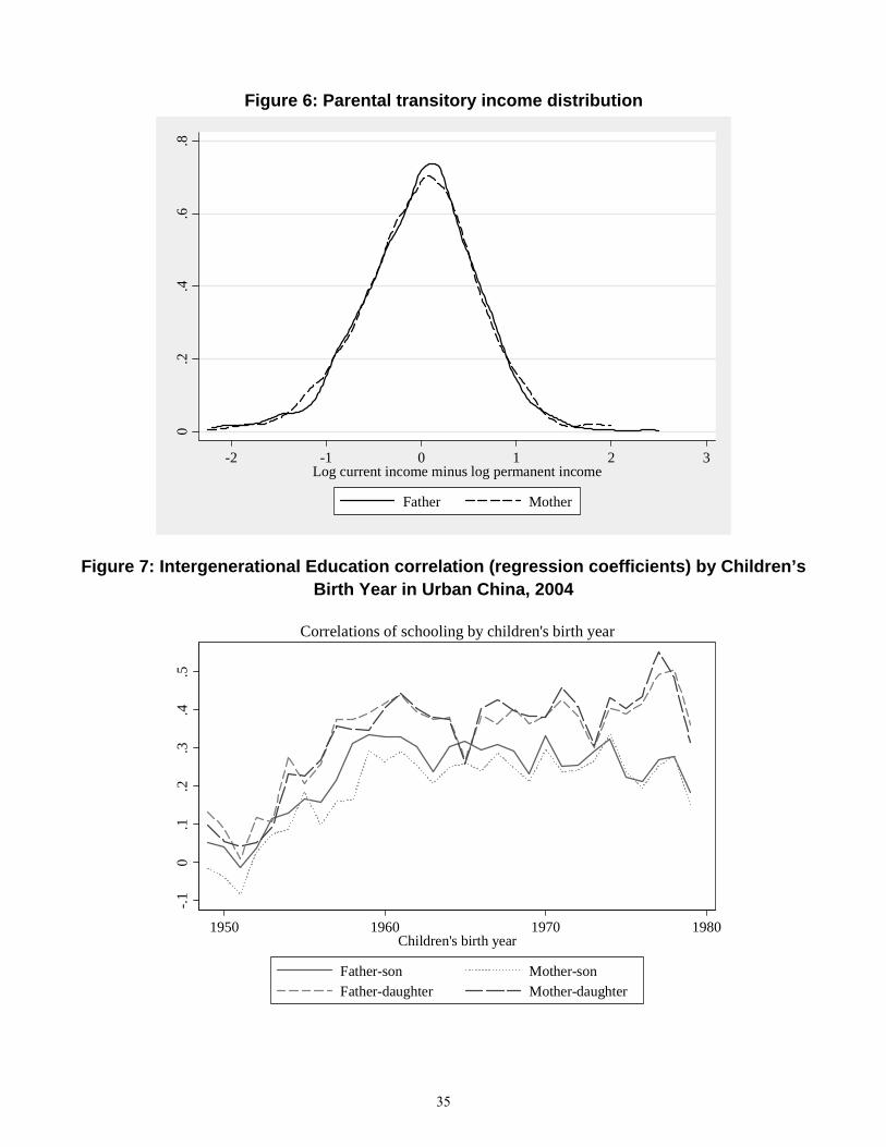
Figure 6: Parental transitory income distribution
0.2
.4.6
.8
-2 -1 0 1 2 3Log current income minus log permanent income
Father Mother
Figure 7: Intergenerational Education correlation (regression coefficients) by Children’s Birth Year in Urban China, 2004
-.10
.1.2
.3.4
.5
1950 1960 1970 1980Children's birth year
Father-son Mother-sonFather-daughter Mother-daughter
Correlations of schooling by children's birth year
35
Father‐sonAll Children Aged >=23 Aged >=30 Aged 30‐42
Children with parents working in 2004
Log(father's income) [IV=occ. & ind.] 0.476 0.471 0.564 0.477 0.466[0.102]*** [0.103]*** [0.130]*** [0.136]*** [0.197]**
Observations 2813 2721 2011 1638 650Father‐daughterLog(father's income) [IV=occ. & ind.] 0.739 0.739 1.013 0.991 0.306
[0.099]*** [0.101]*** [0.135]*** [0.142]*** [0.174]*Observations 2662 2573 1896 1593 595Mother‐sonLog(mother's income) [IV=occ. & ind.] 0.264 0.260 0.337 0.326 0.519
[0.083]*** [0.085]*** [0.112]*** [0.117]*** [0.168]***Observations 1734 1648 1014 909 352Mother‐daughterLog(mother's income) [IV=occ. & ind.] 0.518 0.520 0.711 0.726 0.356
[0.090]*** [0.091]*** [0.129]*** [0.133]*** [0.204]*Observations 1697 1616 1015 944 307
Appendix A: Intergenerational mobility elasticities using permanent parental income with occupation/industry as instruments
Parents‐sonLog(parental income) [IV=occ. & ind.] 0.263 0.262 0.26 0.234 0.243
[0.045]*** [0.046]*** [0.052]*** [0.055]*** [0.114]**Observations 2813 2721 2011 1638 650Parents‐daughterLog(parental income) [IV=occ. & ind.] 0.396 0.371 0.423 0.413 0.151
[0.049]*** [0.049]*** [0.060]*** [0.061]*** [0.103]Observations 2662 2573 1896 1593 595
Robust standard errors in brackets. * significant at 10%; ** significant at 5%; *** significant at 1%Father's income and mother's income are permanent incomes (see text for details). Each elasticity is from a separate regression.
36
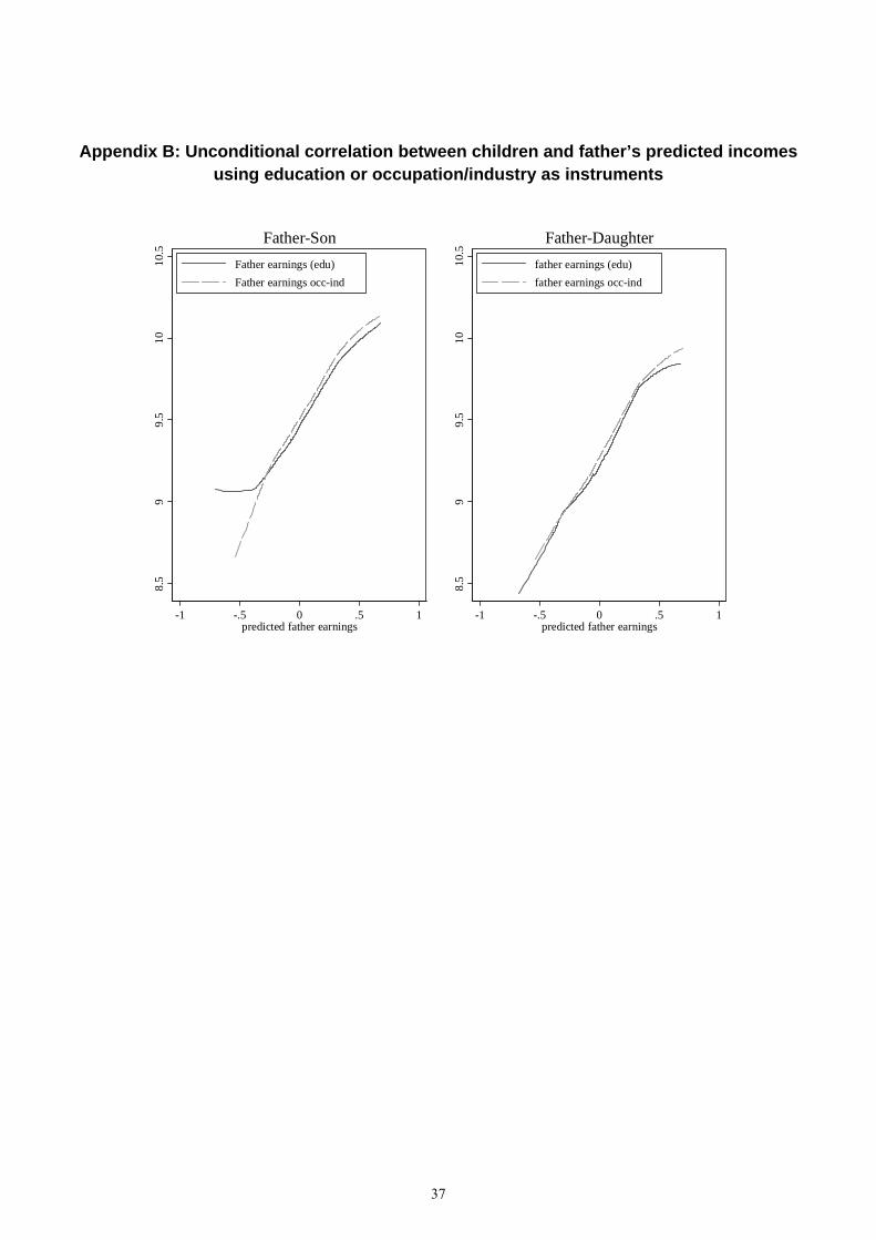
Appendix B: Unconditional correlation between children and father’s predicted incomes using education or occupation/industry as instruments
8.5
99.
510
10.5
-1 -.5 0 .5 1predicted father earnings
Father earnings (edu)Father earnings occ-ind
Father-Son
8.5
99.
510
10.5
-1 -.5 0 .5 1predicted father earnings
father earnings (edu)father earnings occ-ind
Father-Daughter
37