INTERGENERATIONAL AND INTERNATIONAL WELFARE LEAKAGES

OF A TARIFF IN A SMALL OPEN ECONOMY *

Leon J.H. Bettendorf

CPB Netherlands Bureau for Economic Policy Analysis

Ben J. Heijdra

University of Amsterdam, Tilburg University, Tinbergen Institute and OCFEB

ABSTRACT

A dynamic overlapping-generations model of a small open economy with imperfect competition in

the goods market is constructed. A tariff increase reduces output and employment and leads to an

appreciation of the real exchange rate both in the impact period and in the new steady state. The

tariff shock has significant intergenerational distribution effects. Old existing generations gain less

than both younger existing generations and future generations. Bond policy neutralizes the

intergenerational inequities and allows the computation of first-best and second-best optimal tariff

rates. The first-best tariff exploits national market power, but the second-best tariff contains a

correction to account for the existence of a potentially suboptimal product subsidy.

JEL codes: E20, F12, L16, H23.

Keywords: monopolistic competition, love of variety, returns to scale, international

trade, industrial policy, intergenerational welfare effects.

January 1998

Corresponding author:Ben J. Heijdra Leon J.H. BettendorfFEE, University of Amsterdam Central Planning BureauRoetersstraat 11 P.O. Box 805101018 WB Amsterdam 2508 GM The HagueThe Netherlands The NetherlandsPhone: +31-20-525-4113 Phone: +31-70-338-3317Fax: +31-20-525-4254 Fax: +31-70-338-3350Email: heijdra@fee.uva.nl Email: ljhb@cpb.nl

*We thank Peter Broer and conference participants of the NAKE Day (Tilburg University, October24, 1997) for their comments.

CONTENTS

1. Introduction

2. A model of perpetual youth and imperfect competition

2.1. Households

2.2. Firms

2.3. The government

2.4. The foreign sector

2.5. Equilibrium and stability

3. The macroeconomic effects of an import tariff

3.1. Long-run effects

3.2. Short-run and transition effects

4. Intergenerational welfare analysis

4.1. Intergenerational welfare effects without bond policy

4.2. Some numerical illustrations

4.3. Intergenerational redistribution policy

5. Conclusions

References

Figure 1. Determination of the real exchange rate

Figure 2. The dynamic effects of an import tariff

Figure 3. The effect of the tariff on output and the real exchange rate

Table 1. Short-run version of the model

Table 2. Log-linearized version of the model

Table 3. The efficiency and intergenerational distribution effects of an import tariff

1. Introduction

The desirability of industrial policy in an economy with increasing returns to scale industries has

been on and off the research agenda’s of both academic economists and policy practitioners at least

since the debate in the 1920s between Frank Graham and Frank Knight (see Flam and Helpman

(1987) for references). With the advent of the so-called New Trade Theory (Krugman, 1990), the

debate has been given a new lease of life. At least two approaches can be distinguished in the

recent literature. The first approach, which is mentioned but not pursued in this paper, is better

known under the name of strategic trade policy.' In this branch of literature, the issue of

industrial policy is studied in a setting of large duopolistic or oligopolistic firms battling for market

share in the international economy (see Brander (1995) for an overview and references).

The second approach studies the issue of industrial policy in a world characterized by

monopolistic competition. In such a setting there is no strategic interaction between firms, and

trade in varieties of a differentiated product takes place between countries. Flam and Helpman

(1987), for example, construct a static model of a small open economy with a monopolistically

competitive production sector. They use the model to study the effects on allocation and welfare of

tariffs, export subsidies, R&D subsidies, and output subsidies. Flam and Helpman (1987, pp. 90-

91) identify three mechanisms by which welfare of domestic agents is increased in a

monopolistically competitive setting. First, an increase in the number of domestic product varieties

expands the range of choice by domestic consumers, who are better off as a result provided they

exhibit a preference for diversity. Second, a policy that increases the home price of domestically

produced varieties has a positive terms of trade effect which increases welfare of domestic

residents. Third, an increase in the output level per domestic firm constitutes a pro-competitive'

effect and thus increases welfare.

Our paper is a contribution to the second approach to industrial policy. Attention is

restricted to the import tariff. In the static model of Flam and Helpman, the introduction of a tariff

increases profits which prompts an increase in the number of domestic firms and raises the prices

charged by domestic firms. The effects on output per firm is ambiguous, but the terms of trade and

welfare of domestic residents both improve as a result (1987, pp. 91-92). Our first objective in this

paper is to further study the precise conditions under which an import tariff is welfare-improving.

Whilst we retain some of the modelling devices of Flam and Helpman (1987), we modify the

analysis in several directions.

One of our modifications is motivated by a recent body of literature in which it has been

shown that the conclusions based on static models can be highly misleading because the element of

-1-

time is missing in such models. In a world populated with infinitely-lived representative' agents,

this is perhaps not such a problem, because the timing only affects when' (but not whether') the

agents bears the costs of, or receives the benefits from, a particular policy measure. In a world

with finitely-lived overlapping generations, however, the timing of the benefits and costs associated

with a particular policy becomes vital. In such a setting a policy measure typically affects both

existing and future generations differently, i.e. there are not only efficiency but also

intergenerational distribution effects that must be considered. Broer and Heijdra (1996), for

example, use a closed-economy model with monopolistic competition to show that stimulation of

production by means of an investment tax credit is feasible but gives rise to a highly uneven

distribution of costs and benefits over generations. In particular, they show that old existing

generations lose out because they suffer a capital loss on their share holdings, whereas younger

generations as well as future generations benefit as a result of the higher wages and larger number

of product varieties on the market. The importance of intergenerational distribution effects in

determining optimal' policy has been demonstrated in a small but growing number of papers on

very diverse topics.1

The second major objective of our paper is therefore to study the import tariff in a

dynamic overlapping-generations economy. We use the perpetual youth approach of Blanchard

(1985), but extend it to a small open economy and endogenize the labour supply decision of

households. Domestic households purchase domestic and foreign product varieties and use the

current account in order to smooth their consumption profiles. The country is small in world

financial markets and thus faces perfect capital mobility. The domestic real interest rate can vary in

the transition period, however, because of movements in the real exchange rate. There are many

small domestic firms producing varieties that are sold at home and abroad. Free exit/entry

eliminates excess profits in the domestic economy and determines the equilibrium number of firms.

Increasing returns to scale exist because an increase in the number of product varieties boosts the

productivity of the variable labour input.

The analysis yields a number of conclusions. First, in contrast to Flam and Helpman’s

(1987) findings, an increase in the tariff reduces output and employment, both in the short run and

in the long run. The reason is that in our model the tariff shock prompts a negative labour supply

response which leads to a reduction in the number of firms. Like Flam and Helpman (1987), we

find that the real exchange rate appreciates both at impact and in the long run.

Second, the import tariff affects generations unequally. Old existing generations gain less

welfare than younger existing generations and future generations. In terms of the basic mechanisms

identified by Flam and Helpman (1987), generations born in the new steady state lose welfare

-2-

because the number of domestic product varieties falls, but gain welfare because of the

improvement in the terms of trade. Due to free entry/exit and the fixed markup, output per firm is

fixed and thus does not contribute towards welfare. A fourth mechanism operates in our model via

the stock of net foreign assets. It is shown that steady-state generations enjoy a net claim on the

rest of the world as a result of the increase in the tariff. This also exerts a positive effect on the

welfare of steady-state generations.

Third, our analysis shows that a suitable bond accompanying the tariff increase can

neutralize the intergenerational distribution effects so that the pure efficiency effects of the tariff

can be studied. In such an egalitarian setting it is possible to study the optimal tariff. It is shown

that the optimal tariff depends not only on national market power' (as in Gros (1987)) but also on

the pre-existing domestic distortion of monopolistic competition. To the extent that the policy

maker has no instrument to combat the domestic monopoly distortion (such as a product subsidy),

the second-best optimum tariff is reduced vis-à-vis its first-best value. Intuitively, output is already

too low due to the domestic monopoly distortion and increasing the tariff only exacerbates this

problem. In the absence of a domestic distortion and/or if the product subsidy is set optimally, the

first-best tariff is aimed at exploiting national market power to the fullest extent possible. Our

model thus yields precise and intuitively understandable prescriptions about the interaction between

the optimum tariff and pre-existing domestic distortions. In this sense it is related to the earlier

work by Johnson (1965) and Bhagwati (1967, 1971).

The remainder of the paper proceeds as follows. In section 2 the model of a small open

economy is developed. In section 3 the macroeconomic allocation effects of an import tariff are

studied, both at impact, during transition, and in the long run. Section 4 is dedicated to the welfare

analysis both without and with bond policy. Finally, section 5 contains some concluding remarks.

2. A model of perpetual youth and imperfect competition

2.1. Households

The basic model of household behaviour builds on the work of Blanchard (1985) and the extension

to the open economy by Giovannini (1988). Beside the endogeneity of labour supply, the main

difference with these two models is the introduction of diversified consumption goods into the

utility function of the agents. This in turn opens the scope for imperfectly competitive behaviour

on the part of producers, which forms the major innovation of this paper.

In this model there is a fixed population of agents each facing a given constant probability

-3-

of death. During their entire life agents have a time endowment of unity which they allocate over

labour and leisure. The utility functional at timet of the representative agent born at timev is

denoted byΛ(v,t) and has the following form:

whereα is the pure rate of time preference (α>0), β is the probability of death (β≥0), andU(v,τ) is

(2.1)Λ(v,t) ≡ ⌡⌠∞

t

logU(v,τ) exp(α β)(t τ) dτ,

sub-utility which depends on leisure, 1-L(v,τ), and consumption of domestic and foreign composite

goods (CD(v,τ) andCF(v,τ), respectively):

with 0<γ≤1 and 0<γD<1.2

(2.2)U(v,τ) ≡ CD(v,τ)γD CF(v,τ)1 γDγ1 L(v,τ)

1 γ,

The domestic economy consists of imperfectly competitive firms that each produce a single

variety of a diversified good. These goods are close but imperfect substitutes in consumption.

Following Spence (1976) and Dixit and Stiglitz (1977) the diversified goods can be aggregated

over existing varieties (1,2,..,N(τ)) in order to obtainCD(v,τ):

whereCD,i(v,τ) is the consumption of domestically produced varietyi in period τ by an agent born

(2.3)CD(v,τ) ≡ N(τ)η

N(τ) 1N(τ)

i 1

CD,i(v,τ)(σC 1)/σC

σC/(σC 1)

, σC>1, η≥1,

in period v (≤τ), σC is the elasticity of substitution between domestically produced varieties of the

differentiated good, andη is a parameter regulating the preference for diversity effect. Ifη>1, the

individual agents exhibit a love of variety, and settingσC>1 ensures that all existing varieties will

in fact be demanded. For the imported composite consumption good the same specification is

chosen.3

where CF,j(v,τ) is the consumption of foreign varietyj and N* is the (fixed) number of foreign

(2.4)CF (v,τ) ≡ N

η

N1

N

j 1

CF, j (v,τ)(σC 1)/σC

σC/(σC 1)

,

varieties. The true price deflators corresponding to (2.3) and (2.4) are:

-4-

wherePD,i(τ) and PF,j(τ) are, respectively, the price of domestic varietyi and foreign varietyj. The

(2.5)

PD (τ) ≡ N(τ) η

N(τ) σC

N(τ)

i 1

PD,i(τ)1 σC

1/(1 σC)

, PF (τ) ≡ Nη

NσC

N

j 1

PF , j(τ)1 σC

1/(1 σC)

,

real exchange rate is defined asE(τ)≡PF(τ)/PD(τ).

The agent’s budget restriction in terms of the domestic price deflatorPD(τ) is equal to:

whereA(τ)≡dA(v,τ)/dτ, r(τ) is the real rate of interest on domestic assets,W(τ) is the real wage rate

(2.6)A(v,τ) r(τ) β A(v,τ) W(τ)L(v,τ) T(τ) CD(v,τ) E(τ) 1 tM(τ) CF (v,τ),

(assumed age-independent for convenience),T(τ) are net lump-sum taxes,tM(τ) is an ad valorem

import tariff, andA(v,τ) are real tangible assets. All tangible assets are perfect substitutes:

where V(τ)K(v,τ) is the real market value ofK(v,τ) units of land in the hands of households of

(2.7)A(v,τ) ≡ B(v,τ) V(τ)K(v,τ) E(τ)F(v,τ),

vintagev, B(v,τ) is the real stock of government bonds, andF(v,τ) denotes real net foreign assets

measured in terms of the foreign good. Full consumptionX(v,τ) is defined as the sum of real

consumption of the composite differentiated goods and the opportunity cost of leisure:

The domestic economy is small in world capital markets, so that the worldreal rate of

(2.8)X(v,τ) ≡ CD(v,τ) E(τ) 1 tM(τ) CF(v,τ) W(τ) 1 L(v,τ) .

interestrF is fixed. The domestic real interest rate is then determined by the familiar no-arbitrage

condition:

whereE(τ)≡dE(τ)/dτ.

(2.9)r(τ) rF E(τ)/E(τ),

Due to the separable structure of preferences, the choice problem for the representative

agent can be solved in two steps. First, the dynamic problem is solved. This leads to an optimal

time profile for full consumption which is described by the agent’s Euler equation:

In the second step full consumption is optimally allocated over its component parts:

(2.10)X(v,τ)X(v,τ)

r(τ) α.

whereγD thus represents the (constant) share of total goods consumption that is spent on domestic

-5-

goods and 1-γ is the spending share of leisure in full consumption.4 Furthermore, the different

(2.11)CD (v,τ) γγDX(v,τ), E(τ) 1 tM(τ) CF(v,τ) γ (1 γD)X(v,τ),

W(τ) 1 L(v,τ) (1 γ)X(v,τ),

varietiesof the domestically produced and imported goods are determined by:

A crucial feature of the Blanchard (1985) model (and all models deriving from it) is the

(2.12)CD,i (v,τ)

CD(v,τ)N(τ) (σC η) ησC

PD,i(τ)

PD(τ)

σC

,CF, j (v,τ)

CF(v,τ)N

(σC η) ησC

PF,j(τ)

PF(τ)

σC

.

simple demographic structure, which enables the aggregation over all currently alive households.

Assuming that at each instance a large cohort of sizeβS is born and thatβS agents die, and

normalisingS to unity, the size of the population is constant and equal to unity and the aggregated

variables can be calculated as the weighted sum of the values for the different generations. For

example, aggregate financial wealth is calculated asA(τ)≡∫-∞τ βA(v,τ)eβ(v-τ)dv. The aggregated values

for the other variables can be obtained in the same fashion. The main equations describing the

behaviour of the aggregated household sector are given (for periodt) by equations (T1.2) and

(T1.9) in Table 1. Equation (T1.2) is the aggregate Euler equation modified for the existence of

overlapping-generations of finitely-lived agents. It has the same form as the Euler equation for

individual households (equation (2.10)) except for the correction term due to the distributional

effects caused by the turnover of generations. Optimal consumptiongrowth is the same for all

generations but older generations have a higher consumptionlevel than younger generations.5

Since existing generations are continually being replaced by newborns, who hold no financial

wealth, aggregate consumption growth is reduced somewhat as a result. The correction term

appearing in (T1.2) thus represents the difference in average full consumption and full consumption

by newborns:6

where A(τ)≡V(τ)+E(τ)F(τ)+B(τ) is aggregate financial wealth and the constant aggregate stock of

(2.13)X(τ)X(τ)

r(τ) α β (α β)

A(τ)X(τ)

X(v,τ)X(v,τ)

β

X(τ) X(τ,τ)X(τ)

,

land has been normalized to unity, i.e.K(τ)=K=1. Throughout the paper we analyze the case in

which initially both the government debt and the stock of foreign assets are zero, i.e.B=F=0

initially. This ensures that initial financial wealth is strictly positive, i.e.A=V>0 initially. Equation

(T1.2) shows that this is consistent with a steady state provided the world interest rate exceeds the

-6-

rate of time preference, i.e.r=rF>α initially. The rising full consumption profile that this implies

ensures that financial wealth is transferred from old to young generations in the steady-state (see

Blanchard, 1985).

2.2. Firms

The economy consists of a single sector characterized by monopolistic competition. Each firm in

this sector faces a demand for its product,YiD(τ), from two sources: the consumption demand from

the households sector (represented byCD,i(τ) which is obtained by aggregating the first expression

in (2.12)), and the demand from the rest of the world (given byCF*

,i(τ) in equation (2.20) below).

There areN(τ) identical domestic firms that each produce one variety of the differentiated product.

The typical firm’s decision on how much inputs to use is based on profit maximisation. There are

increasing returns to scale at the firm level and the gross production function is homogeneous of

degreeλ (≥1) in the two production factors land (Ki(τ)) and labour (Li(τ)):

whereYi(τ) is marketable output, 0<εL<1, andf is fixed cost (f>0) expressed in terms of the firm’s

(2.14)Yi(τ) f ≡ F(Ki(τ),Li(τ)) Li(τ)λεL Ki(τ)λ(1 εL ),

own output. Representative firmi’s profit is defined by:

whereW(τ)PD(τ) is the nominal wage rate,RL(τ)PD(τ) is the nominal rental rate on land, andsP is

(2.15)Πi(τ) ≡ 1 sP PD,i(τ)Y Di (τ) W(τ)PD(τ)Li(τ) RL(τ)PD(τ)Ki(τ),

an ad valoremsubsidy on production.7 The firm chooses its output and price in order to maximize

(2.15) subject to the demand restrictionYi(τ)=YiD(τ)=CD,i(τ)+CF

*,i(τ) and the production function

(2.14). This essentially static decision problem yields the familiar marginal conditions for labour

and land:

where µi(τ)≡εi(τ)/[εi(τ)-1]>1 is the markup andεi(τ)>1 is the (absolute value of the) elasticity of the

(2.16)∂Yi(τ)

∂Li(τ)

µi(τ)W(τ)PD(τ)

PD,i(τ) 1 sP

,∂Yi(τ)

∂Ki(τ)

µi(τ)RL(τ)PD(τ)

PD,i(τ) 1 sP

,

demand curve faced by firmi. In this paper the assumption ofChamberlinian monopolistic

competition is made: competitors’ reactions are deemed to be absent and entry/exit is assumed to

occur until each active firm makes zero excess profit; the well-known tangency solution. In terms

of the present model this implies thatN(τ) changes instantaneously such that existing firms make

no excess-profits. This in turn implies that the markup equals the scale parameter divided by

average productivity, i.e. µi(τ)=λ(Yi(τ)+f)/Yi(τ).

-7-

2.3. The government

The government sector is modelled in a very simple fashion. We abstract from macro features of

government behaviour such as government spending on goods and services, and distortionary taxes

on labour income. The periodic budget identity of the government is:

where T(τ) is the real lump-sum tax levied on the households andY(τ) is a quantity index for

(2.17)B(τ) r(τ)B(τ) sPY(τ) tM(τ)E(τ)CF(τ) T(τ),

national income:

Since the government is expected to remain solvent, the following NPG condition is relevant:

(2.18)Y(τ) ≡

N(τ)

i 1

PD,i(τ)Yi(τ)

PD(τ)N(τ)η

N(τ) 1N(τ)

i 1

Yi(τ)(σC 1)/σC

σC/(σC 1)

.

The government’s budget restriction is obtained by integrating (2.17) forward subject to (2.19).

(2.19)limτ→∞

B(τ) exp

⌡⌠τ

t

r(s)ds 0.

The resulting expression is given (for periodt) in equation (T1.5) in Table 1.

2.4. The foreign sector

The domestic economy has links with the rest of the world through the goods market (via imports

and exports of differentiated products) and through the assets market (domestic households can

hold foreign assets in their portfolios). Since it is assumed that the domestic economy is small

relative to the rest of the world, domestic variables have no impact on foreign macroeconomic

variables. Hence, the export equation contains mainly exogenous variables. For simplicity the

following specification is adopted for the export demand equation:

whereCF* is the exogenous component of export demand. As before, the parameterσC summarizes

(2.20)1/E(τ)σTCF,i(τ) CF N(τ) (σC η) ησC

PD,i(τ)

PD(τ)

σC

, σT≥1,

how well domestically produced varieties can be substituted by the buyers in the rest of the world.

There is also a separate effect of the real exchange rate on aggregate exports which is

parameterised byσT. Note that equation (2.20) can be seen as the rest of the world’s equivalent to

the second expression in equation (2.12) (in aggregate form).8 In view of the aggregate version of

-8-

the first expression in (2.12) and (2.20) it is clear thatεi(τ)=σC so that the common markup of

domestic firms is constant and equal to µ=µi(τ)=σC/(σC-1)>1.

The change in net foreign assets is equal to the current account. Since net foreign assets,

F(τ), are measured in terms of foreign goods, the balance of payments equation can be expressed

(for period t) as in equation (T1.4) in Table 1. The first term on the right-hand side is foreign

capital income, whilst the second term is real export earnings in terms of the foreign composite

good.

2.5. Equilibrium and stability

The value of the fixed stock of land can be deduced by appealing to the arbitrage equation

between the different tangible assets. The total stock of land is fixed (atK=1) and the market price

of land in terms of the domestic composite good is denoted byV(τ). Land attracts the market rate

of return:

The return on land consists of a capital gain,V(τ), plus the rental received from the imperfectly

(2.21)V(τ) RL(τ)

V(τ)r(τ).

competitive sector,RL(τ), all expressed in terms of the initial price of the land. By solving (2.21)

forward (subject to a transversality condition), the real market price of land can be expressed as the

appropriately discounted value of the stream of rental income:

As is conventional in the macroeconomic literature on imperfect competition, attention is

(2.22)V(t) ≡ ⌡⌠∞

t

RL(τ)exp

⌡⌠τ

t

r(µ)dµ dτ.

restricted to the symmetric equilibrium in which all firms behave in an identical fashion, i.e.

PD,i(τ)=P(τ), CD,i(τ)=CD(τ), Yi(τ)=Y(τ), Li(τ)=L(τ), Ki(τ)=K(τ), and CF*

,i(τ)=CF*(τ) for all domestic

firms (i=1,2,..,N(τ)), and PF,j(τ)=PF, and CF,j(τ)=CF(τ) for all foreign firms (j=1,2,...,N*). Since the

price and number of foreign varieties of the differentiated good are both fixed, a suitable

normalisation ensures that the price indexPF(τ) equals unity. Under symmetry the model can be

rewritten in aggregate terms.

The complete dynamic model is given in aggregated form in Table 1. The dynamic part of

the model is given by equations (T1.1)-(T1.5). The value of one unit of land evolves according to

(T1.1), which is obtained by rewriting (2.21). The movement of full consumption (T1.2), the

uncovered interest parity condition (T1.3), the balance of payments equation (T1.4), and the

-9-

government solvency condition (T1.5) have all been discussed above.

The static part of the model is given by equations (T1.6)-(T1.10). The aggregate demand

for labour depends positively on the output index (given in (2.18)), and negatively on the real

wage rate. The expression for the rental rate on land is given in (T1.7). Land owners receive the

output left over after the factor labour has been paid. The equilibrium condition for the domestic

market for differentiated goods is written in aggregate form in (T1.8). The private demands for the

composite domestic and foreign good and labour supply are given in (T1.9). Finally, the aggregate

production function for the differentiated goods sector is given in (T1.10). It is the aggregated

version of (2.14), where use has been made of the zero pure profit condition.9

The model is given in log-linearized form in Table 2. A tilde ( ~') above a variable

denotes its rate of change around the initial steady-state,e.g., X(t)≡dX(t)/X. A variable with a tilde

and a dot is the time derivative expressed in terms of the initial steady-state, for example,

X.(t)≡X(t)/X. The only exceptions to that convention refer to the tariff, the various financial assets,

and lump-sum taxes: tM(t)≡dtM(t)/(1+tM), V(t)≡rFdV(t)/Y, V.(t)≡rFV(t)/Y, B(t)≡rFdB(t)/Y, B

.(t)

≡rFB(t)/Y, F(t)≡rFdF(t)/Y, F.(t)≡rFF(t)/Y, andT(t)≡dT(t)/Y.

The model can be reduced to a three-dimensional system of first-order differential

equations in net foreign assets,F(t), the value of land,V(t), and full consumption,X(t). Of these

state variables, the net foreign asset position is predetermined, whilst the value of land and full

consumption are non-predetermined jump' variables. Conditional upon the state variables, the

static part of the log-linearized model, consisting of equations (T2.6)-(T2.10) in Table 2, can be

used to derive the following quasi-reduced form' expressions:

(2.23)Y(t) ηεLL(t) W(t) L(t) RL(t) (φ 1)X(t),

(2.24)σTωXE(t) (φ ωX) X(t),

where ωX≡ECF/Y=CF*EσT/Y=(1-γD)/(1+γDtM) is the initial share of international trade (viz. imports

(2.25)σTωX CF(t) tM(t) φ (σT 1)ωX X(t),

equals exports) in aggregate output. The composite parameterφ represents the strength of the

labour supply effect (due to intertemporal substitution) on aggregate domestic output. It is defined

as follows:

-10-

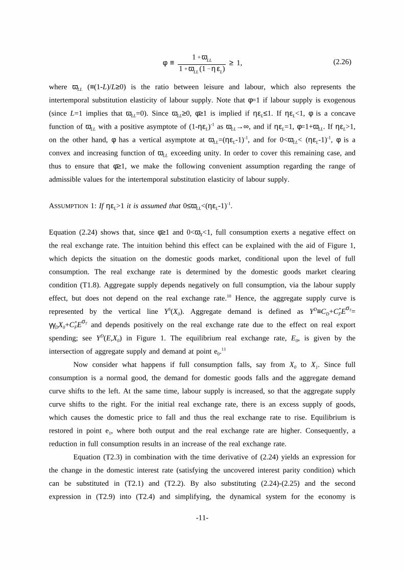
where ωLL (≡(1-L)/L≥0) is the ratio between leisure and labour, which also represents the

(2.26)φ ≡1 ωLL

1 ωLL (1 ηεL)≥ 1,

intertemporal substitution elasticity of labour supply. Note thatφ=1 if labour supply is exogenous

(since L=1 implies thatωLL=0). SinceωLL≥0, φ≥1 is implied if ηεL≤1. If ηεL<1, φ is a concave

function of ωLL with a positive asymptote of (1-ηεL)-1 as ωLL→∞, and if ηεL=1, φ=1+ωLL. If ηεL>1,

on the other hand,φ has a vertical asymptote atωLL=(ηεL-1)-1, and for 0<ωLL< (ηεL-1)-1, φ is a

convex and increasing function ofωLL exceeding unity. In order to cover this remaining case, and

thus to ensure thatφ≥1, we make the following convenient assumption regarding the range of

admissible values for the intertemporal substitution elasticity of labour supply.

ASSUMPTION1: If ηεL>1 it is assumed that0≤ωLL<(ηεL-1)-1.

Equation (2.24) shows that, sinceφ≥1 and 0<ωX<1, full consumption exerts a negative effect on

the real exchange rate. The intuition behind this effect can be explained with the aid of Figure 1,

which depicts the situation on the domestic goods market, conditional upon the level of full

consumption. The real exchange rate is determined by the domestic goods market clearing

condition (T1.8). Aggregate supply depends negatively on full consumption, via the labour supply

effect, but does not depend on the real exchange rate.10 Hence, the aggregate supply curve is

represented by the vertical lineYS(X0). Aggregate demand is defined asYD≡CD+CF*EσT=

γγDX0+CF*EσT and depends positively on the real exchange rate due to the effect on real export

spending; seeYD(E,X0) in Figure 1. The equilibrium real exchange rate,E0, is given by the

intersection of aggregate supply and demand at point e0.11

Now consider what happens if full consumption falls, say fromX0 to X1. Since full

consumption is a normal good, the demand for domestic goods falls and the aggregate demand

curve shifts to the left. At the same time, labour supply is increased, so that the aggregate supply

curve shifts to the right. For the initial real exchange rate, there is an excess supply of goods,

which causes the domestic price to fall and thus the real exchange rate to rise. Equilibrium is

restored in point e1, where both output and the real exchange rate are higher. Consequently, a

reduction in full consumption results in an increase of the real exchange rate.

Equation (T2.3) in combination with the time derivative of (2.24) yields an expression for

the change in the domestic interest rate (satisfying the uncovered interest parity condition) which

can be substituted in (T2.1) and (T2.2). By also substituting (2.24)-(2.25) and the second

expression in (T2.9) into (T2.4) and simplifying, the dynamical system for the economy is

-11-

obtained:

where the Jacobian matrix on the right-hand side,∆, is defined as:

(2.27)

F.(t)

V.(t)

X.(t)

∆

F(t)

V(t)

X(t)

Γ(t),

and whereζ≡σTωX/[φ+(σT-1)ωX], 0<ζ<1. The (potentially time-varying) shock term appearing in

(2.28)∆ ≡

rF 0 φ rF

(rF α) (1 ζ) rF (rF α) (1 ζ) ωK rF (φ 1) (rF α) (1 ζ)

(rF α)ζ /ωK (rF α)ζ /ωK (rF α)ζ

,

(2.27),Γ(t), is defined as:

The model is saddle-point stable provided∆ has two positive (unstable) characteristic roots (r1*>0

(2.29)Γ(t) ≡

ωX

0

0

rF tM(t)

0

(1 ζ)

ζ /ωK

(rF α) B(t).

and r2*>0) and one negative (stable) root (-h*<0). Since the product of the characteristic roots equals

the determinant of∆, stability thus requires that ∆ be negative. After some elementary

operations we find that this is indeed the case:

where the feasible range for the initial product subsidy is such that the share of land owners in

(2.30)∆ ≡ h r1 r2 r 2F φ (ζ /ωK) (rF α) (1 ωK) < 0,

aggregate income lies strictly between zero and unity, i.e. -1<sP<εL/(1-εL) ensures that 0<ωK<1.

Proposition 1 summarizes some results that can be derived for the model.

PROPOSITION 1: Let -1<sP<εL/(1-εL). The loglinearized model of Table 2 implies the following

results: (i) The model is locally saddle-point stable; (ii) The characteristic roots are distinct and

equal to r1*=rF, r2

*>0, and -h*<0. (iii) The second unstable root satisfies r2*>2rF-α. PROOF: See

Bettendorf and Heijdra (1998).

-12-

3. The macroeconomic effects of an import tariff

In this section we study the allocation effects of an unanticipated and permanent increase of the

import tariff. The time at which the policy shock occurs is normalized to zero (hence,tM(t)=tM >0

for t≥0). We assume that no debt policy is used and that the tariff revenue is rebated in a lump-

sum fashion to households. Since both public debt and net foreign assets are zero in the initial

situation (B=F=0), the trade balance is in equilibrium and the only durable asset that is used by

agents to transfer resources intertemporally in the initial steady state consists of claims to domestic

land.

In order to explain the intuition behind the results, we use the diagrammatic apparatus of

Figure 2, in which the exact long-run model solution plus the approximate transitional dynamics

are studied. The first equation in (2.27) explains the time path of net foreign assets and can be

written as follows:

where φ is given in (2.26). In the steady state,F.(t)=0, and (3.1) represents the current account

(3.1)F.(t) rF F(t) φ X(t) ωXtM ,

equilibrium locus, which has been drawn as the CA schedule in Figure 2. This schedule is upward

sloping because, as net foreign assets rise the country receives more interest income from the rest

of the world. In order to restore current account equilibrium domestic households must spend more

on foreign goods. This is established via a rise in full consumption.

The second and third equations of (2.27) show that the dynamic paths for full consumption

and the value of domestic land depend on all three state variables. A full graphical analysis of the

transition path would thus necessitate a three-dimensional graph. To explain the basic intuition we

reduce this dimensionality by basing the graphical analysis (butnot the analytical results) on the

assumption that adjustment in land values occurs fully at impact, i.e.V(t)=V(∞) for t≥0. The

steady-state version of equation of (2.27) furnishes the expression for the steady-state effect of the

tariff on the value of domestic land:

which shows that, provided labour supply is endogenous (φ>1), the value of domestic land

(3.2)V(∞)ωK ωX(φ 1) tM

φ (1 ωK)< 0,

decreases in the long-run. By substitutingV(t)=V(∞) into the third equation in (2.27) the following

expression for the modified Euler equation is obtained:

-13-

In the steady-state,X.(t)=0, and (3.3) represents the modified Keynes-Ramsey rule, which has been

(3.3)X.(t) (rF α) (ζ /ωK) ωKX(t) F(t) V(∞) .

drawn as the MKR schedule in Figure 2.12 This schedule is upward sloping because, in the long

run, the domestic rate of interest is equal to the exogenous world rate. This implies, by (2.13), that

the long-run ratio of financial assets to full consumption,A(∞)/X(∞), is constant also. Hence,

ceteris paribus the value of land, an increase in net foreign assets must be accompanied by an

increase in full consumption.

3.1. Long-run effects

Since an increase in the tariff decreases the long-run value of land (see (3.2)) the MKR locus shifts

down as agents are poorer. The CA curve shifts to the left because ceteris paribus, an increase in

the tariff reduces imports and thus creates a trade balance surplus. In terms of Figure 2, the old

equilibrium e0 lies below the new CA line. In the long run, the economy settles in the new

equilibrium e1 which features a positive net foreign asset position, i.e. a net claim on the rest of the

world, and a higher level of full consumption:

The long-run effects on employment, output, and the rental price of land can be obtained

(3.4)F(∞)ωK ωXtM

1 ωK

> 0, X(∞)ωXtM

φ (1 ωK)> 0.

by using (3.4) and (2.23):

which shows that the effects are strictly negative if labour supply is endogenous (φ>1). Since there

(3.5)Y(∞) ηεLL(∞) RL(∞)ωX(φ 1) tM

φ (1 ωK)≤ 0,

is no long-run effect on the domestic interest rate due to the perfect mobility of financial capital

(r(∞)=0), the long-run effect on the rental price of land is proportional to the effect on land values

(given in (3.2)).

The long-run effect on the wage rate is theoretically ambiguous and depends on the

relative strength of the diversity effectη. Indeed, by using (2.23) and (3.4) we obtain:

With exogenous labour supply (φ=1) or a sufficiently strong diversity effect (ηεL=1), wages are

(3.6)W(∞)(ηεL 1)(φ 1)ωXtM

φηεL (1 ωK).

unaffected by the tariff. In the first case, the labour supply curve is vertical and does not shift,

-14-

whereas in the second case the labour demand curve is horizontal as the marginal productivity of

labour is constant. If the diversity effect is stronger (η>1/εL) the demand for labour is upward

sloping, and if labour supply is endogenous (φ>1), the real wage falls as a result of the tariff.

Under perfect competition the diversity effect is absent (η=1) and the real wage must rise in the

long run.13

The long-run effect on the real exchange rate can be computed by using (2.24) and (3.4):

The effect can be illustrated with the aid of Figure 3. If labour supply is exogenous (φ=1), output

(3.7)E(∞)(φ ωX) tM

φσT(1 ωK)< 0.

supply is fixed. Since full consumption rises, however, the aggregate demand curve is shifted to

the right as the demand for home goods by domestic agents increases. As a result, equilibrium is

restored with an unchanged output level and a lower (appreciated) real exchange rate. In terms of

Figure 3, the equilibrium shifts from e0 to e1. If labour supply is endogenous (φ>1), the increase in

the tariff shifts the aggregate supply curve fromYS(X0) to YS(X1) and the net result of the tariff

increase is a move from e0 to e2, where both output and the real exchange rate are lower.

3.2. Short-run and transition effects

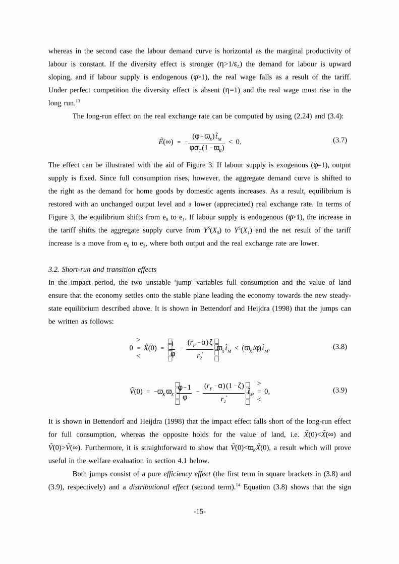
In the impact period, the two unstable jump' variables full consumption and the value of land

ensure that the economy settles onto the stable plane leading the economy towards the new steady-

state equilibrium described above. It is shown in Bettendorf and Heijdra (1998) that the jumps can

be written as follows:

It is shown in Bettendorf and Heijdra (1998) that the impact effect falls short of the long-run effect

(3.8)0>

<X(0)

1φ

(rF α)ζ

r2

ωXtM < (ωX/φ) tM,

(3.9)V(0) ωK ωX

φ 1φ

(rF α) (1 ζ)

r2

tM

>

<0,

for full consumption, whereas the opposite holds for the value of land, i.e.X(0)<X(∞) and

V(0)>V(∞). Furthermore, it is straightforward to show thatV(0)<ωKX(0), a result which will prove

useful in the welfare evaluation in section 4.1 below.

Both jumps consist of a pureefficiency effect(the first term in square brackets in (3.8) and

(3.9), respectively) and adistributional effect(second term).14 Equation (3.8) shows that the sign

-15-

of the full consumption jump is theoretically ambiguous because the efficiency and distributional

effects work in opposite directions. There are strong presumptions, however, that the first effect

dominates andX(0) is positive for all but extremely pathological cases. A number of non-

pathological special cases can be shown in support of this claim. First, if labour supply is

exogenous (φ=1), then the term in square brackets on the right-hand side of (3.8) is positive,

because 0<ζ<1 and r2*>rF-α (see Proposition 1(iii)). The same conclusion holds ifφ is not too

large', which is the case if the diversity effect is not too strong'. Second, ifσT=1 then 0<ζφ=ωX<0

so thatr2*>(rF-α)ζφ regardless of the magnitude of the labour supply parameterφ. Again, the same

conclusion holds for values ofσT that are not too large. It can be demonstrated numerically that

X(0)<0 if the diversity effect is extremely strongand the export elasticity is much larger than

unity. In order to avoid having to deal with this theoretical curiosum, we make the following

assumption regarding the productφζ:

ASSUMPTION 2: If φ,σT>1 it is assumed that the efficiency effect of a tariff dominates the

distributional effect in full consumption, i.e. the parameters are such that r2*>(rF-α)ζφ.

In a similar fashion, the impact jump in the value of land is ambiguous because the efficiency

effect is non-positive and the distributional effect is positive, so that the net effect depends on the

magnitude of the labour supply parameterφ. If labour supply is exogenous (φ=1), then output does

not change as a result of the tariff shock, the efficiency effect is zero, and the value of land

increases at impact due to the distributional effect. On the other hand, if labour supply is

sufficiently elastic (φ>2), then land values fall at impact because the efficiency effect dominates the

distributional effect (see Bettendorf and Heijdra (1998)). Sinceφ>2 does not represent a

particularly outlandish scenario, we conclude that the impact effect on the value of land is

inherently ambiguous for realistic values of the parameters.

Further intuition regarding theexact impact results of (3.8)-(3.9) can be obtained by

appealing to theapproximatetransition dynamics illustrated in Figure 2, which is based on the

assumption that the impact and long-run effects on the value of land are equal to each other (see

above).15 With that approximation, the phase diagram can be constructed as in Figure 2. From

(3.3) it is clear that points above (below) the MKR curve are associated with a rising (falling) full

consumption profile. Similarly, (3.1) shows that points to the right (left) of the CA line are

associated with a current account surplus (deficit) and consequently with an increase (decrease) in

net foreign assets. The approximate saddle path lies between the CA and MKR lines, and is

upward sloping. At impact, the economy jumps from e0 to e′, at which point a current account

-16-

surplus is opened up. During adjustment, net foreign assets and full consumption gradually increase

toward their respective long-run equilibrium levels associated with point e1.

The impact effects on output, employment, and factor prices are obtained by using (2.23)

and (3.8):

With endogenous labour supply (φ>1), both output and employment fall at impact as a result of the

(3.10)Y(0) ηεLL(0) RL(0) 1 1/(ηεL)1W(0) (φ 1)X(0) ≤ 0.

increase in the tariff. The decrease in employment results in a reduction in the marginal product of

land which explains the fall in the rental price of land. The impact effect on the wage rate is

ambiguous and depends on the relative strength of the diversity effect, as was explained above for

the long run. Irrespective of market configuration, however, with endogenous labour supply (φ>1)

the wage-rental ratio unambiguously rises, i.e. the adverse effect on factor payments is worse for

landlords than for labourers. Indeed, by using (3.10) we obtain:

The incidence of the import tariff on factor prices is thus largest for the production factor that is

(3.11)W(0) RL(0)

φ 1ηεL

X(0) > 0.

most elastic in supply which, in the present model, is the factor land.

The impact effect on the real exchange rate is computed by using (2.24) and (3.8):

In Figure 3, the impact effect on output and the real exchange rate is represented by the move

(3.12)σTωXE(0) (φ ωX) X(0) < 0.

from the initial equilibrium at e0 to point e′. Ceteris paribus, the impact appreciation of the real

exchange rate reduces exports and stimulates imports. Furthermore, the increase in full

consumption boosts imports whilst the increase in the tariff reduces imports. Bettendorf and

Heijdra (1998) show that the net impact effect on imports is negative. Since exports fall by less

than imports, the effect on net exports is unambiguously positive. Indeed, by using (2.25) and

(3.12) in (3.1) we obtain the following expression:

where we have used the fact that the stock of net foreign assets is predetermined in the impact

(3.13)r 1

F F.(0) ωX (σT 1)E(0) CF(0) φ X(0) ωXtM > 0,

period (F(0)=0), as well as the upper bound forX(0) in (3.8).

A similar type of reasoning can be used to show that the impact effect on the domestic real

interest rate is negative. Indeed, by using (T2.3) and the time derivative of (2.24), the following

-17-

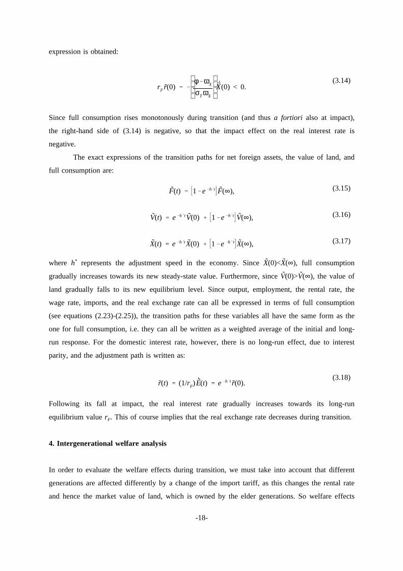
expression is obtained:

Since full consumption rises monotonously during transition (and thusa fortiori also at impact),

(3.14)rF r(0)

φ ωX

σTωX

X.(0) < 0.

the right-hand side of (3.14) is negative, so that the impact effect on the real interest rate is

negative.

The exact expressions of the transition paths for net foreign assets, the value of land, and

full consumption are:

where h* represents the adjustment speed in the economy. SinceX(0)<X(∞), full consumption

(3.15)F(t) 1 e h t F(∞),

(3.16)V(t) e h t V(0) 1 e h t V(∞),

(3.17)X(t) e h t X(0) 1 e h t X(∞),

gradually increases towards its new steady-state value. Furthermore, sinceV(0)>V(∞), the value of

land gradually falls to its new equilibrium level. Since output, employment, the rental rate, the

wage rate, imports, and the real exchange rate can all be expressed in terms of full consumption

(see equations (2.23)-(2.25)), the transition paths for these variables all have the same form as the

one for full consumption, i.e. they can all be written as a weighted average of the initial and long-

run response. For the domestic interest rate, however, there is no long-run effect, due to interest

parity, and the adjustment path is written as:

Following its fall at impact, the real interest rate gradually increases towards its long-run

(3.18)r(t) (1/rF) E

.(t) e h t r(0).

equilibrium valuerF. This of course implies that the real exchange rate decreases during transition.

4. Intergenerational welfare analysis

In order to evaluate the welfare effects during transition, we must take into account that different

generations are affected differently by a change of the import tariff, as this changes the rental rate

and hence the market value of land, which is owned by the elder generations. So welfare effects

-18-

contain both efficiency aspects and generational distribution aspects. In order to link the allocation

effects of the previous section to the welfare effects in this section, the cost-of-living index,PU(τ),

is used to relate sub-utility to full consumption:

whereU(v,τ) is sub-utility defined in (2.2),X(v,τ) is full consumption defined in (2.8) andPU(τ) is

(4.1)U(v,τ) X(v,τ)PU(τ)

,

the cost-of-living index:

where Ω1 is a positive constant. Equation (4.2) shows that increases in the real wage, the real

(4.2)PU(τ) ≡ Ω1 E(τ) 1 tM(τ)γ (1 γD)

W(τ)1 γ,

exchange rate, or the tariff all lead to an increase in the cost-of-living index. In view of (4.1) a

change in sub-utility can thus be decomposed into a term due to a change in full consumption and

a change in the cost-of-living index. This decomposition is useful to explain the intuition behind

the welfare effect on different generations.

4.1. Intergenerational welfare effects without bond policy

To bring out the main issues clearly, we first study the case where no debt policy is used, i.e.

B(t)=0 ∀t≥0. The welfare effect on generations that exist at the time of the shock (t=0) is denoted

by dΛ(v,0), with v≤0. It is shown in Bettendorf and Heijdra (1998) that this effect can be written

as follows:

whereX(v,0)≡dX(v,0)/X(v,0) is the jump at impact in the level of full consumption by a household

(4.3)(α β)dΛ(v,0) X(v,0) rF r ,α β (α β) PU ,α β , v≤0,

of generationv, and r,α+β and PU,α+β represent the Laplace transforms of the paths ofr(t)

and PU(t)≡dPU(t)/PU, respectively, withα+β acting as the discount factor (see below).16 The full-

consumption effect,X(v,0), can be re-written as follows:

whereωH is the initial economy-wide share of human wealth in total wealth (0<ωH<1) andV(0) is

(4.4)X(v,0) V(0)/ωK (1/ωH)e (rF α)v X(0) V(0)/ωK , v≤0,

the change in the value of land that occurs as a result of the change of the import tariff (see (3.9)).

Equation (4.4) implies that the full-consumption jump is increasing in the generations indexv, i.e.

∂X(v,0)/∂v>0.17 The intuition behind this result is as follows. The increase in the import tariff

-19-

gives rise to additional lump-sum transfers. Since all generations have the same expected remaining

lifetime the present value of these additional transfers is the same for all generations. This implies

that all existing generations enjoy the same effect on human wealth and thus, on that account,

increase their full consumption by the same absolute amount. Since old generations are, however,

much wealthier than young generations, this human wealth effect is much more important to the

latter generations.

The second and third terms on the right-hand side of (4.5) affect all existing generations

equally. The second term represents the growth in full consumption. Since all generations are on

an Euler equation of the form (2.10), the path of the interest rate affects all existing generations in

the same way. Finally, the third term represents the cost-of-living effect which simply links full

consumption to sub-utility (see (4.1) above).

In view of equation (4.3)-(4.4), dΛ(v,0) can be written as a weighted average of the effect

on an extremely old generation, dΛ(-∞,0), and the effect on a newborn, dΛ(0,0):

Furthermore, in view of the fact that∂X(v,0)/∂v>0, equation (4.5) implies that dΛ(-∞,0)< dΛ(0,0)

(4.5)dΛ(v,0) 1 e (rF α)v dΛ( ∞,0) e (rF α)vdΛ(0,0), v≤0.

as the welfare effect on existing generations is monotonically decreasing in age, i.e.∂dΛ(v,0)/∂v>0.

Whilst it is thus straightforward to give a relative ranking of the effects on the different

generations, it is not possible to determine analytically the absolute effects on the generations. The

reason for this ambiguity can be clarified by studying the component parts that make up the total

welfare effect. A close inspection of (4.4) reveals that the sign of the full consumption jump,

X(v,0), is ambiguous in general. On the one hand, if labour supply is exogenous (φ=1), thenV(0)>0

(see (3.9)) andX(v,0)>0 for all v, but on the other hand for higher values ofφ, V(0) will be

negative and henceX(v,0)<0 for some generationsv. In the latter case the effect on the level of full

consumption of extremely old generations is negative due to the capital loss they suffer on land.

Since aggregate full-consumption increases at impact (see (3.8) and note Assumption 2), this

implies that the effect on newborns’ full consumption must be positive.

The growth term for full consumption is unambiguously negative. It was shown in the

previous section that the domestic interest rate falls at impact after which it returns to its initial

level during transition (see (3.18)). This implies that the Laplace transform for the path of the

interest rate has the following form:

(4.6) r ,α β ≡ r(0)

α β h< 0.

-20-

The cost-of-living term can be written as a weighted average of the initial and long-run

effect on the cost-of-living index:

The ambiguity of the sign of the cost-of-living term is obvious in view of the fact that the impact

(4.7) PU ,α β ≡PU(0) PU(∞)

α β h

PU(∞)

α β>< 0.

and long-run effects on both the wage and the tariff-inclusive real exchange rate are ambiguous.

Only for some special cases more can be said about the components of PU,α+β. For example,

if labour supply is exogenous (φ=1) or the diversity effect is sufficiently strong (ηεL>1) it can be

demonstrated that the cost-of-living index falls over time, i.e.PU(∞)>PU(0) in that case.

The results in (4.4)-(4.7) thus show that the welfare effect on existing generations is

difficult to sign unambiguously due to the fact that the different components are themselves

ambiguous or work in different directions from each other. It is possible, however, to determine a

relative ranking of the welfare effects on presentand future generations. Future generations are

born in a world that is different from the initial steady state as a result of the shock. The change in

welfare that future generations experience is evaluated at birth, i.e. the relevant indicator is dΛ(t,t)

for v=t≥0. It is shown in Bettendorf and Heijdra (1998) that this welfare indicator can be written as

a weighted average of the effect on a newborn, dΛ(0,0), and the effect on a generation born in the

new steady state, dΛ(∞,∞):

where dΛ(0,0) is obtained from (4.3)-(4.4) by settingv=0, and dΛ(∞,∞) is given by:

(4.8)dΛ(t ,t) e h t dΛ(0 ,0) 1 e h t dΛ(∞,∞), t v≥0,

It is shown in Bettendorf and Heijdra (1998) that the generations born in the new steady-state are

(4.9)(α β)dΛ(∞,∞) X(∞) PU(∞).

better off than very old generations, i.e. dΛ(-∞,0)<dΛ(∞,∞). The reason is that these generations

experience a higher full consumption level (X(∞)>X(0)) which is not offset by cost-of-living

changes. Numerical simulations strongly suggest that dΛ(0,0)<dΛ(∞,∞) although we have been

unable to prove this result unambiguously.18

The main characteristics of the path of (the change of) utility have been summarised in

Proposition 2.

PROPOSITION 2. The solution paths for utility given in(4.5) and (4.8) satisfy the following

properties: (i) The change in welfare of an existing generation depends negatively on its year of

-21-

birth v, i.e., dΛ(-∞,0)<dΛ(0,0); (ii) Old existing generations gain less than future steady-state

generations, i.e.,dΛ(-∞,0)<dΛ(∞,∞). PROOF: See Bettendorf and Heijdra (1998).

4.2. Some numerical illustrations

As was shown in section 3 above, the macroeconomic effects of an import tariff consist of a

gradual accumulation of foreign assets, and a gradual increase in full consumption. However, it is

not in general possible to determine the sign of the welfare effects on current and future

generations. For that reason, we further illustrate Proposition 2 with the aid of some numerical

simulations with a plausibly calibrated version of the model.

Since we wish to study the effects on the intergenerational distribution of the initial tariff

(tM), the strength of the preference for diversity effect (as summarized byη), the export elasticity

(σT), the degree of openness' of the economy (as summarized by 1-γD), and the pre-existing

product subsidy (sP), the model is calibrated in such a way that these parameters can be freely

varied. The parameters that are held fixed throughout the simulations are the rate of pure time

preference (α=0.02), the birth rate (β=0.06), and the efficiency parameter of labour (εL=0.7). The

world interest rate (rF) and the productivity index (Ω0) are used as calibration parameters. For

given values of tM, η, σT, γD, and sP, it is then possible to compute all relevant remaining

information.19

Table 3 presents a number of welfare indicators for different values oftM in the different

rows. Panel (a) of Table 3 is devoted to investigating the effect of the diversity parameterη on the

distribution of welfare, whilst panels (b) through (e) do the same forσT, γD, and sP, respectively.

Consider panel (a) fortM=0 initially. The intergenerational distribution of welfare is very uneven.

Very old existing agents lose substantially (dΛ(-∞,0)<0) but newborns at the time of the shock as

well as all future generation gains unambiguously (dΛ(0,0)>0 and dΛ(∞,∞)>0, so that (4.8) shows

that dΛ(t,t)>0 for all t≥0). This pattern is preserved for all values ofη considered provided the pre-

existing tariff is not too high (tM≤0.3, see the first three rows of Table 3, panel (a)).

Hence, the simulations demonstrate that, for a wide range of values ofη and tM, very old

generations lose whereas young generations gain as a result of an increase in the tariff. But how

does the change in the import tariff affect the population alive at the time of the shock? In order to

answer that question we computeσ(%), which represents the percentage of the population (alive at

the time of the shock) which is no worse-off as a result of the tariff shock. In view of equation

(4.5), σ(%) can be written as:

This variable can be interpreted as the degree of political support that exists for the introduction of

a tariff (if tM=0 initially), or for a marginal increase of the tariff (iftM>0 initially). Indeed, ifσ(%)

-22-

exceeds fifty percent one would expect the existing population to vote in favour of introducing (or

(4.10)σ(%) ≡ 100

1

dΛ( ∞,0)dΛ( ∞,0) dΛ(0,0)

β/(rF α)

.

increasing) the tariff. The information in panel (a) of Table 3 suggests that the degree of political

support decreases with the diversity parameterη. For example, iftM=0 initially, political support is

above fifty percent forη≤1.2 but is below fifty percent for larger values ofη. This shows that,

provided the diversity effect is sufficiently strong, the uneven intergenerational burden can make

the introduction of a tariff unattractive to existing generations.

The second conclusion that can be drawn from panel (a) of Table 3 concerns the effect of

a pre-existing tariff. Raising the initial value oftM drags down the welfare profile for most present

generations and all future generations. As a result, political support declines as the pre-existing

tariff is raised. For example, iftM=0.1 andη=1.0, there is not enough political support for a further

increase in the tariff. Even though the young continue to gain from such a further increase, too

many older generations lose out in this case.

In panel (b) of Table 3 the effect of the export elasticity on the intergenerational welfare

distribution is studied. Three main conclusions emerge from these simulation results. First, raising

σT decreases the gains to all generations. The intuition behind this result is that a higher value for

σT reduces the terms of trade gains. The second conclusion that can be drawn is that for low values

of σT there exists quite substantial political support for a high tariff. For example, ifσT=1 (first

column), even iftM=0.9 initially, there is still a majority among existing generations in favour of a

higher tariff. In that case the country as a whole has a lot of market power (in the sense of Gros

(1987)), and can therefore obtain a substantial appreciation of its real exchange rate at the expense

of foreigners. The third conclusion is that, like in the previous case, political support declines with

the pre-existing tariff.

In panel (c) of Table 3, the effect of the degree of openness of the economy is investigated

numerically. Two major conclusions can be drawn from these results. First, reducing the trade

share (raisingγD) reduces the welfare loss for extremely old generations, and reduces the welfare

gain by generations born in the new steady-state. The effect on newly-born generations is

ambiguous. If tM is low initially, these generations’ gains are reduced asγD rises, whereas the

opposite conclusion holds iftM is high. Political support increases withγD. The intuition behind this

result is that a relatively closed economy has a smaller scope to obtain a welfare transfer from the

rest of the world by means of terms of trade gains that are caused by the tariff. The second

conclusion that can be drawn is that, as in the previous two cases, raising the initial tariff reduces

-23-

political support.

In panel (d) of Table 3 the effect of the pre-existing product subsidysP is investigated. The

main conclusions is that an increase insP leads to an upward shift of the welfare change for all

generations, i.e. it reduces the welfare losses to old generations, and increases the gains to both

newborns and all future generations. The reason is that the product subsidy helps to boost

employment and output and thus leads to a reduction in the severity of the domestic distortion due

to monopolistic competition (see Bettendorf and Heijdra (1996)). This suggests that there exists a

complementarity between the instruments of trade policy (tM) and industrial policy (sP).

4.3. Intergenerational redistribution policy

In the previous section it has been demonstrated that the welfare effect of a supposedly

efficiency-improving' policy measure is generation-dependent, and may be negative for most or

all present generations. This finding demonstrates the need for a mechanism that provides for a

more even distribution of welfare over generations. Indeed, since most or all gainers' are yet-

unborn and all losers' are alive at the time of the shock, the political system of majority rule

would seem to have an inherent bias against a tariff. The present generations in effect produce an

intergenerational externality by not supporting the introduction of (or further increase in) the tariff.

Generations born in the new steady state are better off both because there are terms of trade gains

and because they enjoy a net claim on the rest of the world.20

In this section we endow the policy maker with the ability to use bond policy in order to

neutralize the intergenerational welfare effects. In doing so the pure efficiency effects' of the

import tariff are brought to the fore. Obviously, since old existing generations lose and future

generations gain in the absence of bond policy, the natural choice is to accumulate public debt by

granting a once-off subsidy to the owners of land at the time of the shock. Since land holdings are

predetermined in the impact period, the proper scheme links the once-off subsidy (sK) to the value

of land, i.e. a member of generationv (<0) receives a subsidy ofsKV(0)K(v,0), the aggregate

outlays on the subsidy issKV(0), and the discrete change in the government’s debt position at

impact is given in log-linearized form byB(0)=-sKV(0). It is shown in Bettendorf and Heijdra

(1998) that, provided the subsidy is set at the appropriate level, no further debt policy is needed to

ensure that the welfare of all generations is affected equally, i.e.B(t)=B(0) for t≥0. The

appropriately conducted bond policy ensures thatB(0)=ωXωKtM, which in turn eliminates all

transitional dynamics from the model.

The allocation effects of the change in the tariff accompanied by the bond policy can be

computed by substitutingB(t)=ωXωKtM into (2.29) and solving for the (impact, transition, and long-

-24-

run) effects on the state variables:

for all t≥0. The expression for full consumption can be combined with (2.23)-(2.25) to obtain the

(4.11)F(t) 0, V(t) ωXωK (φ 1)/φ tM < 0, X(t) (ωX/φ) tM > 0,

effects on the other endogenous variables:

for all t≥0.

(4.12)Y(t) ηεL L(t) RL(t) 1 1/(ηεL)

1W(t) ωX (φ 1)/φ tM < 0, r(t) 0,

σTφ E(t) (φ ωX) tM < 0, φσTCF(t) (φ ωX) (σT 1) tM < 0,

The intuition behind these results can be explained with the aid of Figure 2. As before, the

increase in the tariff shifts the CA and MKR loci from CA0 to CA1 and from MKR0 to MKR1,

respectively. The upward jump in the public debt (B(0)=ωXωKtM>0) does not affect the CA locus

but the MKR locus is shifted to the left, i.e. from MKR1 to MKR2. Due to the once-off subsidy to

landowners the increase in the tariff does not only leave the domestic interest rate unaffected (see

(4.12)) but also raises full consumption by the samerelative amount for all generations (see

(2.13)). This neutralizes the differential welfare effect on all existing generations, i.e. dΛ(v,0)=π for

all v≤0, whereπ is the common welfare gain.

Since the policy also eliminates any transitional dynamics from the economy, all future

generations are affected in exactly the same manner, i.e. dΛ(v,v)=π for all v=t≥0. The level of the

common gain to all generations under this egalitarian policy can thus be computed by using (4.9),

(4.11)-(4.12), and the log-linearized version of (4.2):

where Γ(tM,sP) is a complicated function of the parameters and the pre-existing tariff and product

(4.13)π Γ(tM ,sP) tM ,

subsidy. In order to build up intuition concerning this function, it is useful to consider some special

cases. First, if labour supply is exogenous (φ=γ=1), output is fixed and independent of the product

subsidy, andsP drops out ofΓ(tM,sP) altogether:

This expression immediately suggests that introducing a tariff is beneficial (asΓ(0,sP)>0) and that

(4.14)Γ(tM ,sP) ≡(1 γD)γD 1 tM (σT 1)

σT(1 γD tM), for φ 1.

the first-best optimal tariff (for whichΓ(tMF,sP)=0) is aimed at fully exploiting the national market

power' resulting from the upward sloping export function, i.e.tMF=1/(σT-1).

If labour supply is endogenous (φ>1), matters are much more complicated. Bettendorf and

-25-

Heijdra (1996) show that an increase in the product subsidy (under an egalitarian bond policy)

boosts full consumption, output, employment, the number of product varieties, wages, and the

rental on land, and induces a depreciation of the real exchange rate. The consequence of this is that

the pre-existing product subsidy affectsΓ(tM,sP) directly, so that the issue of the optimal tariff is

complicated by second-best considerations, becausesP may be sub-optimal itself. In order to get a

handle on this problem, we compute the second-best optimal egalitarian product subsidy which

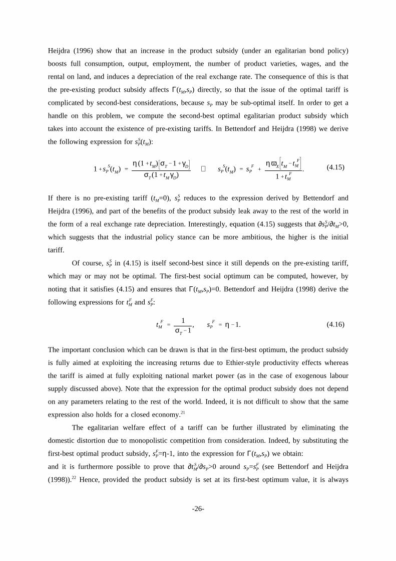
takes into account the existence of pre-existing tariffs. In Bettendorf and Heijdra (1998) we derive

the following expression forsPS(tM):

If there is no pre-existing tariff (tM=0), sPS reduces to the expression derived by Bettendorf and

(4.15)1 s SP (tM)

η (1 tM) σT 1 γD

σT(1 tM γD)⇔ s S

P (tM) s FP

ηωX tM t FM

1 t FM

.

Heijdra (1996), and part of the benefits of the product subsidy leak away to the rest of the world in

the form of a real exchange rate depreciation. Interestingly, equation (4.15) suggests that∂sPS/∂tM>0,

which suggests that the industrial policy stance can be more ambitious, the higher is the initial

tariff.

Of course,sPS in (4.15) is itself second-best since it still depends on the pre-existing tariff,

which may or may not be optimal. The first-best social optimum can be computed, however, by

noting that it satisfies (4.15) and ensures thatΓ(tM,sP)=0. Bettendorf and Heijdra (1998) derive the

following expressions fortMF andsP

F:

The important conclusion which can be drawn is that in the first-best optimum, the product subsidy

(4.16)t FM

1σT 1

, s FP η 1.

is fully aimed at exploiting the increasing returns due to Ethier-style productivity effects whereas

the tariff is aimed at fully exploiting national market power (as in the case of exogenous labour

supply discussed above). Note that the expression for the optimal product subsidy does not depend

on any parameters relating to the rest of the world. Indeed, it is not difficult to show that the same

expression also holds for a closed economy.21

The egalitarian welfare effect of a tariff can be further illustrated by eliminating the

domestic distortion due to monopolistic competition from consideration. Indeed, by substituting the

first-best optimal product subsidy,sPF=η-1, into the expression forΓ(tM,sP) we obtain:

and it is furthermore possible to prove that∂tMS/∂sP>0 aroundsP=sP

F (see Bettendorf and Heijdra

(1998)).22 Hence, provided the product subsidy is set at its first-best optimum value, it is always

-26-

beneficial to introduce a tariff, and as long as the product subsidy is close to its first-best optimum,

(4.17)Γ(tM ,s FP )

γγD (1 γD) 1 tM (σT 1)

σT(1 γD tM),

the second-best optimal tariff depends positively on the pre-existing product subsidy.

We now return to the simulations reported in Table 3. An interesting conclusion that

emerges from this table is that the prudent use of debt policy allows for a more ambitious trade

policy by spreading the costs and benefits equally over all generations. Take, for example, the third

column in panel (a) of Table 3. The diversity effect is equal toη=1.3, and present generations do

not gain sufficiently to vote in favour of even an introduction of a tariff asσ(%)=46.9 for tM=0.

With an egalitarian policy, however, the common gain to all generations is in fact positive

(π=0.333 fortM=0), suggesting that the tariff should be introduced. By shifting some of the benefits

from young and future generations to the older generations, everybody can be made better off. The

same conclusion holds fortM=0.1, and in fact the optimal egalitarian tariff lies somewhere between

tM=0.1 andtM=0.3. The same pattern is observed in the other panels of Table 3.

5. Conclusions

A dynamic overlapping-generations model of a small open economy with monopolistic competition

in the goods market is constructed and analyzed. Industrial policy in the form of an import tariff

reduces output and employment and leads to an appreciation of the real exchange rate both in the

impact period and in the new steady state. An increase in the tariff has important intergenerational

distribution effects. Old existing generations gain less than younger existing generations as well as

future generations. The prudent use of bond policy neutralizes these intergenerational inequities and

suggests first-best and second-best optimal tariff rates. The first-best tariff exploits national market

power, but the second-best tariff contains a correction to account for the existence of a potentially

suboptimal product subsidy.

This paper can be extended in a number of different directions. First, by constructing a

two-country version of the present model the optimal tariff issue can be studied both with and

without international coordination. This would lead to a further clarification of the role of domestic

and foreign scale economies and international market power. It would also forge a link with the

strategic trade policy literature mentioned in the introduction. Our paper, like the traditional

literature, strongly suggests that a tariff increase constitutes a beggar-thy-neighbour policy' which

suggests that international cooperation may lead to a lower optimal tariff. Second, it would be

-27-

desirable to introduce physical capital as a production factor in the present model. A number of

thorny issues must, however, be confronted in such a generalized model. For example, in the

absence of installation costs physical capital is perfectly mobile, leading to implausible impact and

transition effects. See Giovannini (1988) for such a model. Introducing convex installation costs for

investment solves' this problem for the perfectly competitive case (see Buiter (1987)) but opens

an analytically intractable can of worms in a monopolistically competitive world.23 The reason is

that making physical capital imperfectly mobile also breaks the symmetry of the model because

incumbent firms and potential entrants face different costs of producing. The former possess

installed capital and hence face lower costs of adjusting their capital stock than the latter, who

must build up their capital stock from scratch. It is conjectured that a number of first insights into

the effect of capital accumulation on our conclusions can nevertheless be obtained by studying a

version of the model in which there is no entry/exit of firms at all.

-28-

References

Bettendorf, L.J.H. and Heijdra, B.J. (1996). Intergenerational and International Welfare Leakagesof a Product Subsidy in a Small Open Economy.' Tinbergen Institute Discussion Paper, Nr.TI 97-037/2, December.

Bettendorf, L.J.H. and Heijdra, B.J. (1998). Intergenerational and International Welfare Leakagesof a Tariff in a Small Open Economy: Mathematical Appendix.' Mimeo, TinbergenInstitute, University of Amsterdam.

Bhagwati, J.N. (1967). Non-Economic Objectives and the Efficiency Properties of Trade,'Journalof Political Economy, 75, 738-742.

Bhagwati, J.N. (1971). The Generalized Theory of Distortions and Welfare,' in J.N. Bhagwati etal. (eds.), Trade, Balance of Payments and Growth: Essays in Honor of Charles P.Kindleberger, North-Holland, Amsterdam.

Blanchard, O.J. (1985). Debts, Deficits, and Finite Horizons,'Journal of Political Economy, 93,223-247.

Bovenberg, A.L. (1993). Investment Promoting Policies in Open Economies: The Importance ofIntergenerational and International Distributional Effects,'Journal of Public Economics, 51,3-54.

Bovenberg, A.L. (1994). Capital Taxation in the World Economy,' in F. van der Ploeg (ed.),TheHandbook of International Macroeconomics, Basil Blackwell, Oxford, 116-150.

Bovenberg, A.L. and Heijdra, B.J. (1996). Environmental Tax Policy and IntergenerationalDistribution.' OCFEB Research Memorandum 9605, Erasmus University. Forthcoming:Journal of Public Economics.

Brander, J.A. (1995). Strategic Trade Policy,' in G.M. Grossman and K. Rogoff (eds.),Handbookof International Economics, III, Elsevier, Amsterdam, 1395-1455.

Broer, D.P. and Heijdra, B.J. (1996). The Intergenerational Distribution Effects of the InvestmentTax Credit under Monopolistic Competition.' OCFEB Research Memorandum 9603,Erasmus University.

Buiter, W.H. (1987). Fiscal Policy in Open, Interdependent Economies,' in A. Razin and E. Sadka(eds.),Economic Policy in Theory and Practice, Macmillan, London, 101-144.

Dixit, A.K. and Pindyck, R.S. (1994).Investment under Uncertainty, Princeton University Press,New Haven, Conn.

Dixit, A.K. and Stiglitz, J.E. (1977). Monopolistic Competition and Optimum Product Diversity,'American Economic Review, 67, 297-308.

Engel, C. and Kletzer, K. (1990). Tariffs and Saving in a Model with New Generations.'Journalof International Economics, 28, 71-91.

Flam, H. and Helpman, E. (1987). Industrial Policy under Monopolistic Competition.'Journal of

-29-

International Economics, 22, 79-102.

Galor, O. (1994). Tariffs, Income Distribution and Welfare in a Small Open Overlapping-Generations Economy.'International Economic Review, 35, 173-192.

Giovannini, A. (1988). The Real Exchange Rate, the Capital Stock, and Fiscal Policy.'EuropeanEconomic Review, 32, 1747-1767.

Gros, D. (1987). A Note on the Optimal tariff, Retaliation and the Welfare Loss from Tariff Warsin a Framework with Intra-Industry Trade.'Journal of International Economics, 23, 357-367.

Heijdra, B.J. (1994). Fiscal Policy in a Dynamic Model of Monopolistic Competition.' DiscussionPaper No. TI94-133, Tinbergen Institute, University of Amsterdam, October.

Heijdra, B.J. and Van der Ploeg, F. (1996). Keynesian Multipliers and the Cost of Public FundsUnder Monopolistic Competition.'Economic Journal, 106, 1284-1296.

Johnson, H.G. (1965). Optimal Trade Intervention in the Presence of Domestic Distortions,' inR.E. Baldwin et al. (eds.),Trade, Growth, and the Balance of Payments: Essays in Honorof Gottfried Haberler, North-Holland, Amsterdam.

Keuschnigg, C. and Kohler, W. (1996). Commercial Policy and Dynamic Adjustment UnderMonopolistic Competition,'Journal of International Economics, 40, 373-409.

Krugman, P.R. (1990).Rethinking International Trade Theory, MIT Press, Cambridge, Mass.

Spence, M. (1976). Product Selection, Fixed Costs, and Monopolistic Competition.'Review ofEconomic Studies, 43, 217-235.

-30-

Table 1: Short-Run Version of the Model

(T1.1)V(t) r(t)V(t) RL(t)

(T1.2)X(t) r(t) α X(t) β (α β) V(t) E(t)F(t) B(t)

(T1.3)r(t) rF E(t)/E(t)

(T1.4)F(t) rFF(t) CF E σT 1 CF(t)

(T1.5)B(t) ⌡⌠∞

t

T(τ) tM(τ)E(τ)CF(τ) sP(τ)Y(τ) exp

⌡⌠τ

t

r(µ)dµ dτ

(T1.6)εL 1 sP Y(t) W(t)L(t)

(T1.7)(1 εL) 1 sP Y(t) RL(t)

(T1.8)Y(t) CD(t) CF E(t)σT

(T1.9)CD(t) γγDX(t), E(t) 1 tM(t) CF(t) γ (1 γD)X(t), W(t) 1 L(t) (1 γ)X(t)

(T1.10)Y(t) Ω0L(t)ηεL

Notes: (a) PF(t)≡1 andE(t)≡PF(t)/PD(t) is the real exchange rate.(b) Ω0≡(λ/µ)η/λ((µ-λ)/λf)(η-λ)/λ>0.

-31-

Table 2: Log-Linearized Version of the Model

(T2.1)V.(t) rF V(t) rF ωK r(t) RL(t)

(T2.2)X.(t) rF α X(t) rF r(t) (rF α)/ωK V(t) F(t) B(t)

(T2.3)E.(t) rF r(t)

(T2.4)r 1

F F.(t) F(t) ωX (σT 1)E(t) CF(t)

(T2.5)r 1F B(0) T,rF (1 tM)

tM,rF

tM

1 tM

X,rF

(T2.6)L(t) Y(t) W(t)

(T2.7)RL(t) Y(t)

(T2.8)Y(t) (1 ωX) CD(t) ωXσTE(t)

(T2.9)CD(t) X(t), CF(t) CD(t) E(t) tM(t), L(t) ωLL W(t) X(t)

(T2.10)Y(t) ηεL L(t)

Shares:ωLL (1-L)/L Initial leisure/work ratio.ωK RL/Y Initial share of rental income in national income.ωX ECF/Y Initial share of imports (and exports) in national

income.

Notes: (a) We have used the normalizationE=1 and B=F=0 initially. The total (constant)stock of land equalsK=1.

(b) Relationship between shares:ωK=(1-εL)(1+sP), ωX=(1-γD)/(1+γDtM).

Table 3. The Efficiency and Intergenerational Distribution Effectsof an Import Tariff

Panel (a): The effect of the diversity parameter

η=1.0 η=1.2 η=1.3 η=1.4 η=1.6

tM=0.0 πdΛ(-∞,0)dΛ(0,0)dΛ(∞,∞)σ(%)

0.637-5.3041.3392.02556.0

0.434-5.5131.1561.73650.0

0.333-5.6171.0651.59146.9

0.231-5.7220.9741.44743.6

0.029-5.9320.7951.15736.8

tM=0.1 πdΛ(-∞,0)dΛ(0,0)dΛ(∞,∞)σ(%)

0.484-5.1691.0681.83848.9

0.286-5.3720.8881.55542.2

0.187-5.4740.7991.41338.6

0.087-5.5760.7101.27134.9

-0.111-5.7800.5340.98827.1

tM=0.3 πdΛ(-∞,0)dΛ(0,0)dΛ(∞,∞)σ(%)

0.220-4.9320.6321.51134.2

0.031-5.1240.4591.24125.8

-0.063-5.2200.3741.10621.4

-0.158-5.3170.2880.97116.8

-0.347-5.5100.1180.702

7.1

tM=0.5 πdΛ(-∞,0)dΛ(0,0)dΛ(∞,∞)σ(%)

0.000-4.7310.2941.23618.5

-0.179-4.9130.1290.980

8.4

-0.269-5.0040.0470.852

3.1

-0.359-5.095-0.0350.723

0.0

-0.538-5.277-0.1970.467

0.0

tM=0.7 πdΛ(-∞,0)dΛ(0,0)dΛ(∞,∞)σ(%)

-0.186-4.5590.0241.002

1.8

-0.357-4.731-0.1330.759

0.0

-0.442-4.817-0.2110.637

0.0

-0.527-4.903-0.2900.515

0.0

-0.698-5.076-0.4450.272

0.0

tM=0.9 πdΛ(-∞,0)dΛ(0,0)dΛ(∞,∞)σ(%)

-0.346-4.411-0.1960.801

0.0

-0.508-4.574-0.3470.569

0.0

-0.589-4.655-0.4220.453

0.0

-0.670-4.737-0.4960.337

0.0

-0.832-4.900-0.6450.106

0.0

Note: Parameter values areα=0.02,β=0.06,γD=0.5, εL=0.7, sP=0, σT=3, andωLL=2.0. σ(%) is thepercentage of the population (alive at the time of the shock) that does not lose as a result of amarginal increase in the tariff. The efficiency gain under egalitarian redistributive bond policyis given byπ.

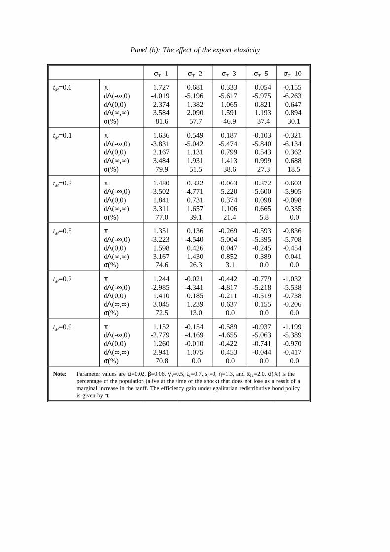
Panel (b): The effect of the export elasticity

σT=1 σT=2 σT=3 σT=5 σT=10

tM=0.0 πdΛ(-∞,0)dΛ(0,0)dΛ(∞,∞)σ(%)

1.727-4.0192.3743.58481.6

0.681-5.1961.3822.09057.7

0.333-5.6171.0651.59146.9

0.054-5.9750.8211.19337.4

-0.155-6.2630.6470.89430.1

tM=0.1 πdΛ(-∞,0)dΛ(0,0)dΛ(∞,∞)σ(%)

1.636-3.8312.1673.48479.9

0.549-5.0421.1311.93151.5

0.187-5.4740.7991.41338.6

-0.103-5.8400.5430.99927.3

-0.321-6.1340.3620.68818.5

tM=0.3 πdΛ(-∞,0)dΛ(0,0)dΛ(∞,∞)σ(%)

1.480-3.5021.8413.31177.0

0.322-4.7710.7311.65739.1

-0.063-5.2200.3741.10621.4

-0.372-5.6000.0980.665

5.8

-0.603-5.905-0.0980.335

0.0

tM=0.5 πdΛ(-∞,0)dΛ(0,0)dΛ(∞,∞)σ(%)

1.351-3.2231.5983.16774.6

0.136-4.5400.4261.43026.3

-0.269-5.0040.0470.852

3.1

-0.593-5.395-0.2450.389

0.0

-0.836-5.708-0.4540.041

0.0

tM=0.7 πdΛ(-∞,0)dΛ(0,0)dΛ(∞,∞)σ(%)

1.244-2.9851.4103.04572.5

-0.021-4.3410.1851.23913.0

-0.442-4.817-0.2110.637

0.0

-0.779-5.218-0.5190.155

0.0

-1.032-5.538-0.738-0.206

0.0

tM=0.9 πdΛ(-∞,0)dΛ(0,0)dΛ(∞,∞)σ(%)

1.152-2.7791.2602.94170.8

-0.154-4.169-0.0101.075

0.0

-0.589-4.655-0.4220.453

0.0

-0.937-5.063-0.741-0.044

0.0

-1.199-5.389-0.970-0.417

0.0

Note: Parameter values areα=0.02,β=0.06,γD=0.5, εL=0.7, sP=0, η=1.3, andωLL=2.0. σ(%) is thepercentage of the population (alive at the time of the shock) that does not lose as a result of amarginal increase in the tariff. The efficiency gain under egalitarian redistributive bond policyis given byπ.

Panel (c): The effect of the trade share

γD=0.1 γD=0.3 γD=0.5 γD=0.7 γD=0.9

tM=0.0 πdΛ(-∞,0)dΛ(0,0)dΛ(∞,∞)σ(%)

0.353-10.625

1.7052.51341.9

0.370-8.0861.4072.09144.3

0.333-5.6171.0651.59146.9

0.241-3.2390.6771.01349.9

0.094-1.0060.2400.35754.1

tM=0.1 πdΛ(-∞,0)dΛ(0,0)dΛ(∞,∞)σ(%)

0.149-10.729

1.2122.32231.4

0.190-8.0201.0321.89534.9

0.187-5.4740.7991.41338.6

0.140-3.1030.5170.88142.6

0.056-0.9500.1860.30447.8

tM=0.3 πdΛ(-∞,0)dΛ(0,0)dΛ(∞,∞)σ(%)

-0.215-10.896

0.3991.97811.3

-0.125-7.8820.4211.54716.2

-0.063-5.2200.3741.10621.4

-0.025-2.8800.2660.66326.9

-0.004-0.8640.1030.22033.5

tM=0.5 πdΛ(-∞,0)dΛ(0,0)dΛ(∞,∞)σ(%)

-0.530-11.019-0.2481.677

0.0

-0.394-7.744-0.0561.246

0.0

-0.269-5.0040.0470.852

3.1

-0.155-2.7040.0770.490

9.3

-0.050-0.7990.0420.15716.7

tM=0.7 πdΛ(-∞,0)dΛ(0,0)dΛ(∞,∞)σ(%)

-0.806-11.108-0.7771.411

0.0

-0.626-7.610-0.4400.983

0.0

-0.442-4.817-0.2110.637

0.0

-0.260-2.562-0.0710.350

0.0

-0.085-0.750-0.0060.108

0.0

tM=0.9 πdΛ(-∞,0)dΛ(0,0)dΛ(∞,∞)σ(%)

-1.051-11.171-1.2211.172

0.0

-0.830-7.481-0.7570.752

0.0

-0.589-4.655-0.4220.453

0.0

-0.347-2.445-0.1890.234

0.0

-0.113-0.710-0.0430.068

0.0

Note: Parameter values areα=0.02,β=0.06,η=1.3, εL=0.7, sP=0, η=1.3, andωLL=2.0. σ(%) is thepercentage of the population (alive at the time of the shock) that does not lose as a result of amarginal increase in the tariff. The efficiency gain under egalitarian redistributive bond policy isgiven byπ.

-35-

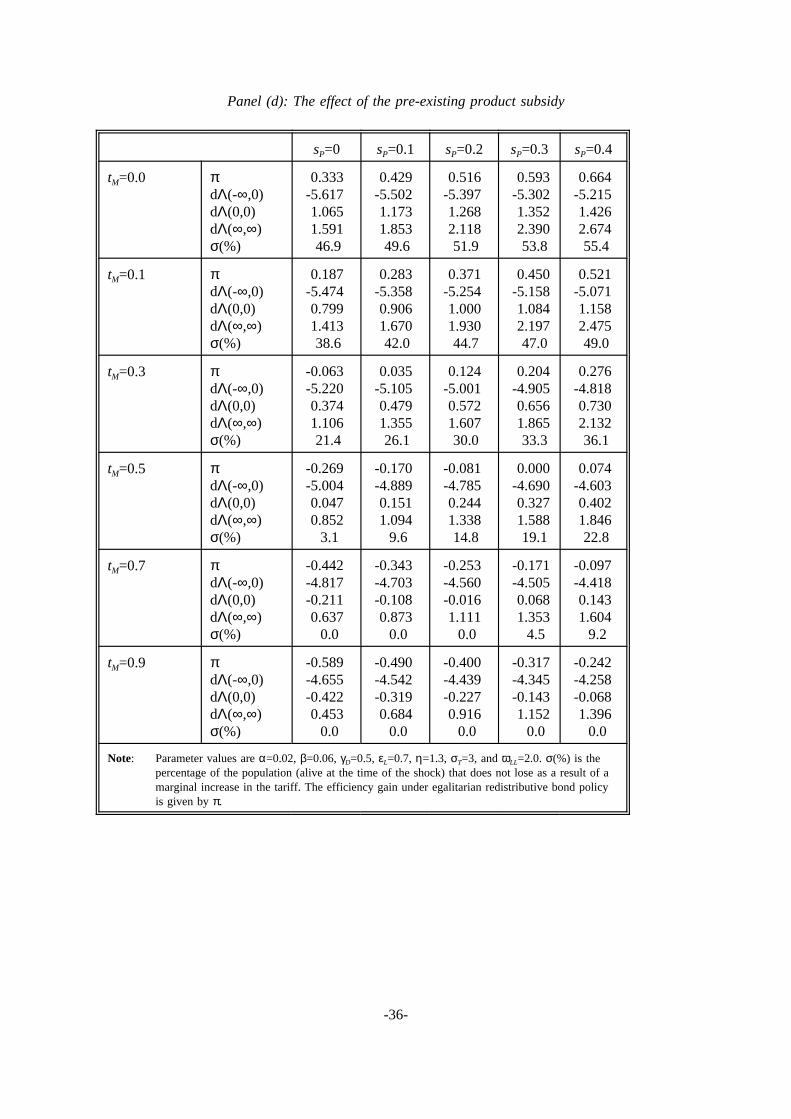
Panel (d): The effect of the pre-existing product subsidy

sP=0 sP=0.1 sP=0.2 sP=0.3 sP=0.4

tM=0.0 πdΛ(-∞,0)dΛ(0,0)dΛ(∞,∞)σ(%)

0.333-5.6171.0651.59146.9

0.429-5.5021.1731.85349.6

0.516-5.3971.2682.11851.9

0.593-5.3021.3522.39053.8

0.664-5.2151.4262.67455.4

tM=0.1 πdΛ(-∞,0)dΛ(0,0)dΛ(∞,∞)σ(%)

0.187-5.4740.7991.41338.6

0.283-5.3580.9061.67042.0

0.371-5.2541.0001.93044.7

0.450-5.1581.0842.19747.0

0.521-5.0711.1582.47549.0

tM=0.3 πdΛ(-∞,0)dΛ(0,0)dΛ(∞,∞)σ(%)

-0.063-5.2200.3741.10621.4

0.035-5.1050.4791.35526.1

0.124-5.0010.5721.60730.0

0.204-4.9050.6561.86533.3

0.276-4.8180.7302.13236.1

tM=0.5 πdΛ(-∞,0)dΛ(0,0)dΛ(∞,∞)σ(%)

-0.269-5.0040.0470.852

3.1

-0.170-4.8890.1511.094

9.6

-0.081-4.7850.2441.33814.8

0.000-4.6900.3271.58819.1

0.074-4.6030.4021.84622.8

tM=0.7 πdΛ(-∞,0)dΛ(0,0)dΛ(∞,∞)σ(%)

-0.442-4.817-0.2110.637

0.0

-0.343-4.703-0.1080.873

0.0

-0.253-4.560-0.0161.111

0.0

-0.171-4.5050.0681.353

4.5

-0.097-4.4180.1431.604

9.2

tM=0.9 πdΛ(-∞,0)dΛ(0,0)dΛ(∞,∞)σ(%)

-0.589-4.655-0.4220.453

0.0

-0.490-4.542-0.3190.684

0.0

-0.400-4.439-0.2270.916

0.0

-0.317-4.345-0.1431.152

0.0

-0.242-4.258-0.0681.396

0.0

Note: Parameter values areα=0.02,β=0.06,γD=0.5, εL=0.7, η=1.3, σT=3, andωLL=2.0. σ(%) is thepercentage of the population (alive at the time of the shock) that does not lose as a result of amarginal increase in the tariff. The efficiency gain under egalitarian redistributive bond policyis given byπ.

-36-

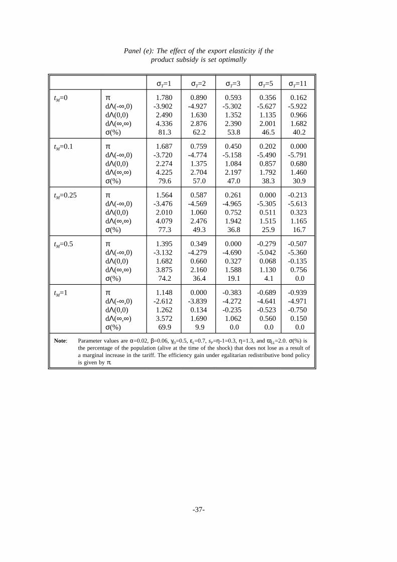
Panel (e): The effect of the export elasticity if theproduct subsidy is set optimally

σT=1 σT=2 σT=3 σT=5 σT=11

tM=0 πdΛ(-∞,0)dΛ(0,0)dΛ(∞,∞)σ(%)

1.780-3.9022.4904.33681.3

0.890-4.9271.6302.87662.2

0.593-5.3021.3522.39053.8

0.356-5.6271.1352.00146.5

0.162-5.9220.9661.68240.2

tM=0.1 πdΛ(-∞,0)dΛ(0,0)dΛ(∞,∞)σ(%)

1.687-3.7202.2744.22579.6

0.759-4.7741.3752.70457.0

0.450-5.1581.0842.19747.0

0.202-5.4900.8571.79238.3

0.000-5.7910.6801.46030.9

tM=0.25 πdΛ(-∞,0)dΛ(0,0)dΛ(∞,∞)σ(%)

1.564-3.4762.0104.07977.3

0.587-4.5691.0602.47649.3

0.261-4.9650.7521.94236.8

0.000-5.3050.5111.51525.9

-0.213-5.6130.3231.16516.7

tM=0.5 πdΛ(-∞,0)dΛ(0,0)dΛ(∞,∞)σ(%)

1.395-3.1321.6823.87574.2

0.349-4.2790.6602.16036.4

0.000-4.6900.3271.58819.1

-0.279-5.0420.0681.130

4.1

-0.507-5.360-0.1350.756

0.0

tM=1 πdΛ(-∞,0)dΛ(0,0)dΛ(∞,∞)σ(%)

1.148-2.6121.2623.57269.9

0.000-3.8390.1341.690

9.9

-0.383-4.272-0.2351.062

0.0

-0.689-4.641-0.5230.560

0.0

-0.939-4.971-0.7500.150

0.0

Note: Parameter values areα=0.02,β=0.06,γD=0.5, εL=0.7, sP=η-1=0.3,η=1.3, andωLL=2.0. σ(%) isthe percentage of the population (alive at the time of the shock) that does not lose as a result ofa marginal increase in the tariff. The efficiency gain under egalitarian redistributive bond policyis given byπ.

-37-

Footnotes

1. Recent examples include Bovenberg (1993) on investment stimulation measures,Bovenberg (1994) on capital taxation, as well as Engel and Kletzer (1990) and Galor(1994) on tariffs. All these papers analyse a small open economy with universal perfectcompetition. Bovenberg and Heijdra (1996) analyse environmental taxes in a closedeconomy. Bettendorf and Heijdra (1996) use the model of this paper to study themacroeconomic and distributional effects of a product subsidy. See also the recent study byKeuschnigg and Kohler (1996).

2. Hence, it is assumed that the Armington substitution elasticity between domestic andforeign composite consumption goods (sayσA) equals unity. This assumption is made forsimplicity. A non-unitary Armington elasticity,σA≠1, does not substantially affect thearguments in this paper.

3. Hence, it is assumed that domestic and foreign varieties substitute equally well amongthemselves. This assumption helps in keeping the model as simple as possible.

4. If γ=1, labour supply is exogenous and each agent inelastically supplies one unit of labour.

5. Provided financial wealth is positive, which is ensured throughout the paper. See below.

6. We use the fact thatX(τ)=(α+β)[A(τ)+H(τ)] and X(τ,τ)=(α+β)H(τ) in the second step.

7. We include a pre-existing product subsidy to capture the notion that the policy maker maybe engaged in industrial policy aimed at correcting for the monopoly distortions in theeconomy. Below we demonstrate the interaction between the optimal tariff and the pre-existing product subsidy. In Bettendorf and Heijdra (1996) we study the allocation andwelfare effects of the product subsidy.

8. This explains the appearance of the term involvingN(τ) in (2.20).

9. Free exit and entry implies that average cost curve is tangent to the demand curve. It isstraightforward to show that marginal cost of any active firm (MCi) equals total cost (TCi)divided by λ times gross production (Y+f), i.e., MCi=TCi/λ(Y+f). The expressions in (2.16)imply the usual mark-up pricing rule, i.e.,P=µMCi. The tangency condition requiresP=ACi=TCi/Y. Combining these conditions yields the zero pure profit condition µY=λ(Y+f).For obvious reasons, this expression is only meaningful if the markup exceeds the scaleparameterλ, i.e. µ>λ is assumed throughout the paper. This condition has been used toderive (T1.10).

10. If the substitution elasticity between broad consumption and leisure (sayσCM) is unequal tounity, the real exchange rate also affects labour supply directly. Indeed, ifσCM>1, laboursupply and hence output depend negatively on the real exchange rate, rendering theaggregate supply curve downward sloping in Figure 1. Nothing of substance is affected byrestricting attention to the Cobb-Douglas case withσCM=1.

11. Note thatYD does not directly depend on the tariff,tM. If the Armington substitutionelasticity between domestic and foreign composite consumption goods (σA) is unequal tounity, the tariff also affects aggregate demand directly. Indeed, ifσA>1, the home demandfor domestic goods and hence aggregate demand depend positively on the tariff. Nothing ofsubstance is affected by restricting attention to the Cobb-Douglas case withσA=1.

-38-

12. The slope of the MKR curve is∂X/∂F=1/ωK and the slope of the CA curve is∂X/∂F=1/φ.Hence, since 0<ωK<1 andφ≥1, the MKR locus is steeper than the CA locus.

13. Under perfect competitionλ=µ=1 andf=0 and the diversity effect is not operative as thenumber of firms is not determined in the model. Hence, the perfectly competitive solutionsare obtained from our model by settingη=1 andΩ0=1. See Heijdra (1994) and Heijdra andvan der Ploeg (1996) for further details.

14. In the representative-agent version of the model,β=0 and rF=α, and only the efficiencyeffect remains.

15. Below we give the expressions for the exact transition paths. See equations (3.15)-(3.17).

16. Intuitively, the Laplace transform x,s denotes the present value of the time pathx(t)usings as the discount factor:

x,s ≡ ⌡⌠∞

0

x(t)e stdt.

17. We use the fact thatX(0)-V(0)/ωK>0. A proof for this result is found in Bettendorf andHeijdra (1998).

18. Despite trying a very wide array of (sometimes very unrealistic) parameter values, we havebeen unable to produce a counterexample to the claim that dΛ(0,0)<dΛ(∞,∞). See alsoTable 3.

19. Specifically, ωK=(1-εL)(1+sP), ωX=(1-γD)/(1+γDtM), 1/γ=1+ωLLεLθM(1+sP), 1/L=1+ωLL,θM≡(1+tMγD)/(1+tM), and

rF r 1

2α α2 4βγ(α β)ωK .

20. These terms of trade gains are needed to create a steady-state deficit on the trade accountin the new steady state. This deficit is covered by interest income received from the rest ofthe world. It is tempting (but incorrect) to view the terms of trade effect and the netforeign asset effect as one and the same thing. It is shown below, however, that it issocially optimal not to allow present generations to accumulate a net claim on the rest ofthe world. It that sense, the terms of trade effect in the absence of bond policy isexcessive', a phenomenon that is represented by the net foreign asset effect.

21. This can be seen by settingγD=1 in (4.15). See also the related paper by Broer and Heijdra(1996).

22. The numerical simulations in Table 3(d) suggest that∂tM* /∂sP>0 may in fact hold globally.

We have been unable to prove this conjecture, however.

23. The installation cost approach to investment has itself been subjected to severe criticism inrecent years. See, for example, Dixit and Pindyck (1994).

-39-

E

E0

YD(E,X0)

YD(E,X1)

E1

e0

e1

e1

e2

Y0 Y1

YS(X1)YS(X0)

Y,YD,YS

Figure 1. Determination of the real exchange rate

Key: E is the real exchange rate, Y is aggregate output, YD is aggregate demand, YS is aggregatesupply, and X is full consumption. A decrease in full consumption, say from X0 to X1, stimulateslabour supply, and the supply curve for goods shifts to the right. Aggregate demand is reduced, asgoods are normal in consumption. At the old real exchange rate E0 there is excess supply of goods,and the real exchange rate depreciates. Equilibrium is restored in e1.

e0

e1

SP

F~

~X

F()~

X(0)~

X()~

e1

0

0

MKR0 MKR1

CA0

CA1

e2

MKR2

Figure 2. The dynamic effects of an import tariff

Key: F is net foreign assets, X is full consumption, MKR is the modified Keynes-Ramsey rule, CA isthe current account equilibrium locus, and SP is the saddle path. An increase in the tariff shifts thelong-run equilibrium from e0 to e1, and full consumption and net foreign assets both rise. Thetransition path is a jump at impact from e0 to e1, followed by gradual adjustment along the saddle pathSP towards e1. With an egalitarian policy the MKR curve shifts to the left and impact and long-runeffects occur at point e2.

E

YD(E,X0)

e0

e2

Y0

YD(E,X1)

YD(E,X2)

e1

E0

e1

YS(X2)YS(X0)YS(X1)

Y,YD,YS

Figure 3. The effects of the tariff on output and the real exchange rate

Key: E is the real exchange rate, Y is aggregate output, YD is aggregate demand, YS is aggregatesupply, and X is full consumption. With exogenous labour supply (3=1), output is fixed and the tariffonly affects aggregate demand via its effect on full consumption which rises in the long run. Theexchange rate appreciates as the equilibrium shifts from e0 to e1. With endogenous labour supply(3>1), there is also a negative effect on the supply of domestic output. The equilibrium shifts from e0

to e2 in that case.