Embed Size (px)
Citation preview

TI 2010-078/3 Tinbergen Institute Discussion Paper
A Meta-Analysis of the Equity Premium
Casper van Ewijka,b,c
Henri L.F. de Groota,c,d Coos Santinge
a CPB Netherlands Bureau for Economic Policy Analysis, The Hague, The Netherlands; b University of Amsterdam, Amsterdam, The Netherlands; c Tinbergen Institute, The Netherlands; d VU University Amsterdam, Amsterdam, The Netherlands; e Ministry of Finance, The Hague, The Netherlands.

Tinbergen Institute The Tinbergen Institute is the institute for economic research of the Erasmus Universiteit Rotterdam, Universiteit van Amsterdam, and Vrije Universiteit Amsterdam. Tinbergen Institute Amsterdam Roetersstraat 31 1018 WB Amsterdam The Netherlands Tel.: +31(0)20 551 3500 Fax: +31(0)20 551 3555 Tinbergen Institute Rotterdam Burg. Oudlaan 50 3062 PA Rotterdam The Netherlands Tel.: +31(0)10 408 8900 Fax: +31(0)10 408 9031 Most TI discussion papers can be downloaded at http://www.tinbergen.nl.

A Meta-Analysis of the Equity Premium
Casper van Ewijk,a,b,c
Henri L.F. de Groota,c,d
and Coos Santinge
a CPB Netherlands Bureau for Economic Policy Analysis, The Hague, The Netherlands
b University of Amsterdam, Amsterdam, The Netherlands c Tinbergen Institute, Amsterdam-Rotterdam, The Netherlands
d Dept. of Spatial Economics, VU University Amsterdam, The Netherlands
e Ministry of Finance, The Hague, The Netherlands
Abstract
The equity premium is a key parameter in asset allocation policies. There is a vigorous debate in the
literature regarding the actual measurement of the equity premium, its size and the determinants of its
variation. This study aims to take stock of this literature by means of a meta-analysis. We identify how
the size of the equity premium depends on the way it is measured, along with its evolution over time
and its variation across regions in the world. We find that the equity premium is significantly lower if
measured by ex ante methods rather than ex post, in more recent periods, and for more developed
countries. In addition, looking at the underlying fundamentals, we find that larger volatility in GDP
growth tends to raise the equity premium while a higher nominal interest rate has a negative impact on
the equity premium.
Keywords: equity premium, meta-analysis
JEL codes: D53, E44, G12, N20
Useful comments by Clemens Kool, Peter Schotman, Bas ter Weel and Ed Westerhout are gratefully acknowledged. We are also grateful to Jan Luiten van Zanden for sharing historical interest rates and inflation rates (from International Institute of Social History) that underly our analysis in Section 4.3. The usual disclaimer applies.

1
1. Introduction: The Equity Premium
The equity premium is a key parameter in asset allocation policies. It measures the excess return above
the risk-free return and as such it can be seen as the price for risk. There has been a lively debate in the
theoretical as well as the empirical literature on the measurement, size and sources of variation of the
equity premium. In their seminal contribution, Mehra and Prescott (1985) identified the famous equity
premium puzzle according to which there is a discrepancy between the equity premium as measured
empirically and the premium that follows from standard theory. Mehra and Prescott calculated a
historical equity premium of 6.2 percent in the United States for the period 1889–1978. Economic
theory, based on the consumption capital asset pricing model (CCAPM), only justifies a premium up
to a maximum of about 0.35 percent using conventional values for risk aversion. Their study initiated
an intense debate in the scientific literature on the determination and size of the equity premium, both
on the theoretical side (cf. Weil, 1989, Kocherlakota, 1996, Campbell and Cochrane, 1999, and many
others) and on the empirical side of the puzzle. This paper focuses on the empirical aspects of the
discussion, and aims to take stock of the existing literature by performing a meta-analysis of a wide
selection of empirical studies on the equity premium, and to explain the sources of variation in this
literature.
Meta-analysis provides us with a toolkit of statistical techniques enabling a quantitative review
of the existing literature. As such, it complements narrative reviews.1 Meta-analysis originated in the
experimental sciences and was later on extended to fields such as the medical sciences where it has
gained the status of a common practise instrument to merge results from different trials on the
effectiveness of a specific drug or treatment. The research method has subsequently been introduced in
psychology and education and is gradually gaining ground in economics (see, e.g., Florax et al., 2002,
for an overview). Nowadays meta-analyses have been performed for a wide array of both
microeconomic and macroeconomic issues. This study adds a new topic to the list which is at the heart
of finance and also has close ties to macroeconomics.
Considering the empirics of the equity premium, four major issues stand out. First, the equity
premium as measured from ex post stock returns proves to be quite sensitive to the observation period.
This even holds for the long periods that are often used to identify the premium, which is obviously
due to the large volatility of stock prices. This causes controversy on the 'true' value of the equity
premium. For example, Siegel (1992) suggests that the high equity premium found by Mehra and
Prescott (1985) was the result of the relatively low risk free rate in the period 1889–1978. Siegel found
that the equity premium in this period is 4% higher than in the two decades just before and after this
1 For good overviews of the literature, see Dimson et al. (2002) and Mehra (2008). See also Fernandez (2009a,b) for studies complementary to our meta-analysis which are based on a survey among professors and a review of information provided in 150 textbooks in finance.

2
period (viz. the periods 1880–1888 and 1979–1990, respectively). Including these adjacent periods
would lower the equity premium by some 0.8% points.
A second, and related, controversy concerns the question whether the equity premium is
constant over time. Several authors suggest that the equity premium is declining over time, especially
since World War II (e.g., Blanchard, 1993, Siegel, 1999, Dimson et al., 2002), whereas others claim
that the equity premium will continue to remain high (e.g., Mehra, 2003).
Third, the equity premium may vary across space. There is no strict need that the equity
premium should be identical across countries and regions. Differences in stage of development leading
to different aggregate risks, or differences in institutions leading to differences in leverage, could well
explain different values of the equity premium. Moreover, as better time series tend to be available for
the more successful stock markets, in particular the United States, this may have caused a bias in
research as well. Jorion and Goetzmann (1999) conclude that the high equity premium obtained for
U.S. equities could be the exception rather than the rule. Extending the data set to other markets –
including the ones that did not survive – they find a lower estimate of the world rate of return on
equity by 0.29 % points. Since that study the scope of research is broadened as more data become
available for other countries. An important study in this respect is the “Triumph of the Optimists” by
Dimson et al. (2002) who have calculated the equity premium for 17 countries over a period of 101
years.
A final issue is whether the equity premium should be measured ex post or ex ante. In ex post
studies the equity premium is calculated as the difference in the mean return on stocks, either taken
geometrically or arithmetically, and the risk free rate, mostly the short term interest rate (T-bills) or
long term government bonds. This ex post approach is taken by Mehra and Prescott (1985) as well as
many others (cf. Siegel, 1999, Dimson et al., 2002). Ex ante studies, in contrast, take the dividend
yield or the earnings-price ratio as a starting point and derive the implied equity premium using an
estimate for the capital gains. Seminal contributions here are Blanchard (1993), and Fama and French
(1988, 2002) who found substantially lower estimates for the equity premium – ranging from 2.5% to
3% in the last study – than in most ex post studies.
After having addressed these issues, our analysis will be extended by looking at some
fundamentals of the equity premium. First, we will have a closer look at the relationship between the
equity premium and the interest rate and the rate of inflation. Next, we will investigate two underlying
macroeconomic determinants. It is typically argued in the literature that the equity premium is higher
in emerging markets than in mature markets (Shackman, 2006, and Erbas and Mirakhor, 2007).
Investing in developing countries is generally perceived to be more risky, which has to be
compensated in terms of a higher return. The stage of development of a country will be proxied by its
Gross Domestic Product (GDP) per capita. Another macroeconomic factor that can influence the
3
equity premium is the size of aggregate risk, here measured by the volatility of GDP growth. It is well
known that higher volatility of consumption leads to higher required returns (Weil, 1989). In this vein
Lettau et al. (2008) provide evidence that decreasing macroeconomic risk explains the boom of the
stock markets in the 1990s. We will consider whether differences in the volatility of the economy
indeed affect the equity premium. In this respect this study may contribute to the understanding of the
impact of the credit crisis on the equity premium, even though the credit crisis itself is beyond the
scope of this study (the most recent paper on the equity premium included in our meta-analysis being
from 2008).
The remainder of this paper is structured as follows. Section 2 discusses several measurement
issues, and identifies potential sources of variation in the equity premium. It thus paves the road for
the selection of moderator variables to be employed in the meta-regression analysis. Section 3
describes the selection process of the primary studies of the meta-analysis and provides summary
statistics of the explanatory variables. Section 4 discusses the results of the meta-regression,
investigates the impact of structural underlying variables, and finally constructs benchmark values for
the equity premium. Section 5 concludes.
2. How to measure the equity premium?
The literature on the equity premium provides no unanimity on how to measure the equity premium.
In theory the equity premium represents the additional risk premium on equity relative to the return on
safe assets. Or, more precisely the equity premium (EP) is defined as difference between the required
return on equity ( er ) and the risk free rate ( fr ):
fe rrEP −≡ . (1)
Assuming market efficiency, the required rate of return equals the expected rate of return (viz.
][ ee rEr = ). There are a number of issues concerning the measurement of the equity premium. First
and most fundamental, there is the difference between ex post and ex ante approaches to estimate the
equity premium. Second, the choice of the market portfolio of stocks may matter for the height of the
equity premium. In general, authors use a wide portfolio corresponding to well-established indices for
official stock markets. Second, as purely safe assets do not exist in practice, one has to find a suitable
proxy for the risk free rate. Third, there is a more technical issue of measuring returns as an arithmetic
or geometric mean. Each of these issues is briefly discussed below.

4
Ex post or ex ante measurement of the equity premium
Mehra and Prescott (1985) measure the equity premium by calculating the historical return on stocks
compared to the risk free rate. This ‘ex post’ approach is followed by many others (e.g., Dimson et al.,
2002). It is not undisputed though. In particular, this method may be biased if the equity premium is
not stationary during the observation period. Rising price earnings ratios over a prolonged period after
World War II (up to the credit crisis) may point to a secular decline in the risk premium on equity.
Indeed, building on Gordon’s (1962) dividend discount model, Blanchard (1993) estimated that the
equity premium in the United States had fallen to 2-3% in the early 1990s. Essentially, this ‘ex ante’
method takes the equity price as the present value of future dividends or earnings. Then, estimating
future growth of earnings (dividends), one can calculate the equity premium implied in observed
earnings to price ratio, or dividend to price ratio. Blanchard’s finding of a declining premium was
confirmed in other ex ante studies such as Jagannathan et al. (2000), and Fama and French (2002).2
The choice in method can thus have substantial consequences for the size of the equity
premium. For the United States, Fama and French (2002) find that the ex-post equity premium for the
period 1951–2001 is almost three times as high as the ex-ante estimate. In a stationary environment
both methods, ex ante and ex post, are expected to converge in the long run. In a non-stationary
environment, however, the outcome can differ for the two methods, even producing seemingly
contradictory results (e.g., Lengwiler, 2004). This is because changes in the required rate of return
produce just the opposite effect on the realised return through the revaluation of stocks. For this reason
Dimson et al. (2002) warn not to extrapolate the high post-war returns into the future. As these high
ex-post returns were caused by the revaluation of stocks due to a fall in the prospective rate of return,
they rather point to low future returns.
Choice of market portfolio
Most authors measure the equity premium using the well-known stock market indices for a broad
market portfolio, such as Standard and Poors for the United States and the MSCI for the developed
countries. Usually midcaps are not included in the data. This may matter, as the equity premium
depends on the risk profile of the companies, and also on the equity-debt composition in financing the
firm. Higher risk and higher leverage imply higher returns on equity. As most authors use broad
market portfolios, we will make no further distinction with regard to the portfolio in the meta-analysis.
When using long time series one should furthermore be aware of the sensitivity of the results for
2 Early ‘ex ante’ studies focused on the equity premium per se. Others have extended this framework by allowing the projected growth of dividends and earnings to depend on other variables. This leads to the so-called conditional model of the equity premium, as distinct from the unconditional model employed by, for example, Fama and French (2002). Claus and Thomas (2001) use several accounting variables to do this. Earlier, Blanchard (1993) used the unconditional dividend model, but took account of expectations of the interest rate and inflation rate.

5
survivorship of companies over time. If indexes are constructed by only including companies that are
present today, a bias is created since companies that went bankrupt are excluded by construction
(Brown et al., 1995). However, the general idea is that survivorship bias in stock market returns is
small. In our meta-analysis we will therefore neglect the potential influence of ‘survivorship bias’.
However, Jorion and Goetzmann point out that there may exist a survival bias across stock markets as
well, as existing long data series tend to focus on markets that have been successful up to date. Also,
time series often break down during deep crises such as wars and revolutions. Indeed, the very focus
in research on the most successful stock market, viz. the United States, may lead to a significant bias.
Constructing data for other stock markets Jorion and Goetzmann show that U.S. equities have the
highest return over the period 1921–1996, at 4.3%, versus a mean return for other countries in the
sample of only 0.8%. Taking the average of all countries, including these other markets, lowers the
world market return by 0.29% points relative to the U.S. return.
Risk free rate
The second important measurement issue concerns the choice of the risk free rate. In theory, a risk free
asset should deliver an income flow in real terms that is independent of the state of the world
(Lengwiler, 2004). Unfortunately such an asset does not exist. Government paper comes closest, as it
has low default risk.3 Therefore, most studies on the equity premium use the return on short term
treasury bills or long term bonds as a proxy for the risk free rate. A disadvantage of such assets is that
their real return depends on inflation. Inflation-indexed governments bonds do exist, but are only
recently available. Economists therefore prefer treasury bills (T-bills) or notes with a short time to
maturity, as they are less sensitive to inflation and interest rate risk. Others, however, prefer long term
bonds, as this is more in line with the long-term character of equity.4 The impact of the risk-free asset
against which the equity premium is determined will be identified in the meta-analysis by using a
dummy indicating whether the risk-free rate is proxied by T-bills (short-term) or long-term bonds.5
Arithmetic versus geometric measurement of mean returns
Using historical time series, the return on equity can be calculated as a geometric mean (GR) or an
arithmetic mean (AR). The difference relates to the way in which series of returns are averaged over
time. If returns are measured arithmetically, the average is taken as the sum of the returns per period
3 In deep crises, such as wars and revolutions, also governments may default on their liabilities. For this reason Jorion and Goetzmann (1999) focus on real equity return, that is the return relative to commodities, rather than on the equity premium which measures the return relative to government debt. 4 Recently, some work is being done on the term structure of the equity premium (cf. Lemke and Werner, 2009). In this meta-analysis we will take account of the term of the risk free rate, but ignore potential differences in the equity premium arising from a term structure as knowledge on this is still pre-mature. 5 See Dimson et al. (2007) for an extensive discussion on the impact of maturity of the risk free rate on the equity premium.

6
divided by the number of periods. If returns are measured geometrically this is calculated as the
compound rate of return (Derrig and Orr, 2003). Arithmetic returns tend to be higher than the
geometric returns. With lognormal returns the expected geometric return (GR) converges to the
expected arithmetic return minus half the variance, that is GR = AR – ½ σ2 (see, e.g., Welch, 2000,
Dimson et al., 2002, and Ibbotson and Chen, 2002). The arithmetic mean is generally considered to
produce the best estimate of the mean return; the geometric mean approximates the median return
rather than the mean (Campbell et al., 1997, Jacquier et al., 2003, and Ten Cate, 2009). In the meta-
regression model the difference between the arithmetic and geometric return is captured by a simple
dummy variable.
3. Data Sources and Summary Statistics
This section describes the selection of the studies that are used in our meta-analysis, and provides a
brief characterization of the database by some descriptive statistics. The formal meta-regression model
and its results will be presented in the next section. The equity premium puzzle that was identified by
Mehra and Prescott (1985) resulted in a flood of studies on the equity premium, both theoretical and
empirical. We focus on the empirical studies. To construct the database for the meta-analysis, we
started using the search engine Econlit covering published articles in English in academic journals.6
The keywords used for our search were ‘equity premium’. This resulted in 242 hits of which 15
studies measure the size of the equity premium. Using the technique of snowballing (see, for example,
Cooper and Hedges, 1994), nine other studies were found which were added to the database. We are
thus left with 24 studies that form the heart of our meta-analysis. Each study reports several equity
premiums, covering different time periods, countries and methodologies.7 The resulting database
consists of 535 observations. Appendix A provides a list of all studies and their summary statistics.
The studies are also clearly marked in the list of references.
Clearly, the database is not balanced across the spatial and time dimension. In the spatial
distribution, there is a bias towards developed countries, in particular the United States. Over the past
couple of years, however, the sample of countries for which equity risk premiums are available has
increased substantially due to, for example, studies by Dimson et al. (2002), Shackman (2005), and
Salomons and Grootveld (2003). In total, our database includes 44 countries. Almost half of the
observations (256) refer to the United States. For many other countries, there is only a couple of
observations available. We therefore combine these countries into relatively homogeneous regions,
viz. Canada, Oceania (Australia, New Zealand and Japan), Canada, Western Europe, Advanced
6 Econlit American Economic Association’s electronic bibliography contains 750 journals since 1962 (see www.econlit.org). 7 There are studies reporting premiums covering a broad time span as well as premiums for sub-periods within this broad time span. In these cases, the former is omitted from the analysis to avoid double counting.

7
Emerging Countries (including amongst others Brazil, Mexico, Poland and South Africa), Secondary
Emerging Countries (including amongst others Argentina, China, India, Turkey), and the Asian
Tigers.8
Across the temporal dimension there is a bias towards more recent periods. Some studies
cover a long time span of almost two centuries (from 1830 to present), but most studies cover more
recent periods. About 9% of the observations is characterized by a mid-year before 1900. About 13%
has a mid-year that falls in the period 1900–1950. For the remaining 78%, the mid-year is 1950 or
later.9 Concerning the way of measurement, over 80% of the observations measure the equity premium
on an ex post basis. Furthermore, the majority concerns equity premiums that are measured
arithmetically (354 compared to 181 on a geometric basis).10 Finally, of the 535 observations, 310 are
calculated with T-bills or closely related substitutes. The other 225 equity premiums are calculated
with bonds proxying for the risk free asset.
3.1 Descriptive analysis of the data
The within-study distribution of the observations is presented in Figure 1. For each individual study it
gives the minimum and maximum value of the equity premium along with a 95% confidence
interval.11 The primary studies are ordered according to the within-study variation measured by the
size of the 95% confidence interval.
According to Figure 1, some studies in the meta-analysis report negative equity premiums
(viz. Blanchard et al., 1993, Canova and Nicolo, 2003, Digby et al., 2006, Fama and French, 2002,
Jagannathan et al., 2000, Salomons and Grootveld, 2003, Shackman, 2006, Siegel, 2005, Ville, 2006,
and Vivian, 2007). There are also very large equity premiums as is the case for the study by Salomons
and Grootveld (2003). We see large differences for the within-study variation of the equity premium.
For Dimson et al. (2006), the lower bound of the 95% confidence interval is 5.0% and the upper bound
is 6.0%. In contrast, for Mehra and Prescott (1985) the lower bound is 1.9% and the upper bound is
10.5%.
8 Further details on country groupings are available upon request. 9 The mid-year is the average of the initial and final year of the period covered by the observation. 10 If studies do not report the method to calculate returns the arithmetic one is assumed. We performed a robustness check to investigate the sensitivity for this assumption. Details are available upon request from the authors. 11 The confidence interval of the mean is equal to the within study mean plus or minus two times the within study standard-deviation divided by the square root of the number of observations.

8
Figure 1. Within- and between-study variation of the Equity Premium
-30
-20
-10
0
10
20
30
40
50
Note: lines indicate minimum and maximum EP’s found in the respective studies. The boxes indicate a 95% confidence
interval around the mean of the respective studies.
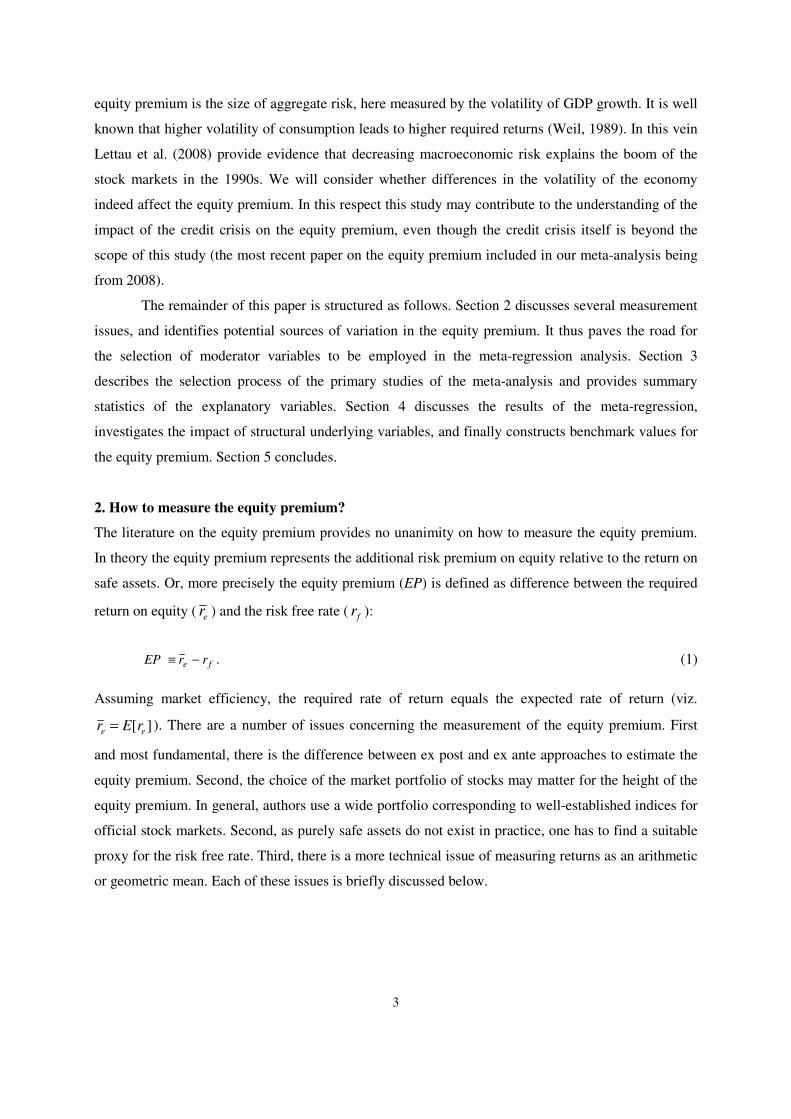
Figure 2 further describes the distribution of the equity premium for the entire sample of 535
observations. The mean is 5.73. The null-hypothesis of a normal distribution is clearly rejected (p-
value <0.001). There are 24 observations with a negative equity premium, whereas 48 observations
have equity premiums exceeding 10%.
9
Figure 2. Histogram the Equity Premium
0
10
20
30
40
50
60
70
80
-20 -15 -10 -5 0 5 10 15 20 25 30 35 40 45
Time Variation
Figure 3 gives an impression of the temporal variation of the equity premium. More precisely, each
observation is expressed for the mid-year of the period on which this observation is based. This figure
confirms the overall picture that the equity premium was low until 1920, high in the 1920s and again
high in the post war period. Short term deviations from this overall pattern are observed in the 1970s
(with a dip and a recovery thereafter). The recent crisis on the financial markets falls beyond the scope
of all studies included in the sample.12
12 It should be noted that this is not a complete representation of the variation of the equity premium over time. As the data points refer to the mid year of observation periods with different lengths, the evolution of the equity premium is smoothed. Restricting the dataset to only observation periods of 10 years or less, shows a similar pattern but with greater volatility. Looking at the length of the period studied in somewhat greater detail, we can distinguish several categories, viz. 0–10 years (123 observations), 11–20 years (66 observations), 21–30 years (79 observations), 31–50 years (51 observations), 51–100 years (110 observations) and more than 100 years (106 observations). In our database, there are no observations based on periods shorter than 5 years or longer than 203 years. Further details on the impact of differences in the length of the observation period are available upon request from the authors.
Mean: 5.73
Median: 5.29
St.dev.: 4.35
Skewness: 1.78
Kurtosis: 20.11

10
Figure 3. Variation over time in the equity premium by mid year of the observation period
-30
-20
-10
0
10
20
30
40
50
Note: lines indicate minimum and maximum EP’s found in the respective periods. The boxes indicate a 95% confidence
interval around the mean of the respective regions. The number of observations for each period is indicated in brackets.
Spatial Variation
The equity premium also varies considerably over space as is shown in Figure 4. To obtain a more
balanced set, some countries are grouped into relatively homogeneous groups. We find that the equity
premium is relatively high in emerging countries. The lowest average equity premium is found in
Canada, and the highest is found for the Asian Tigers. The mean of the equity premium for these
groups of countries varies from 3.95 percent in Canada to 13.14 in the Asian Tigers.

11
Figure 4. The Equity Premium by Country or Region
-30
-20
-10
0
10
20
30
40
50
Canada (22) USA (256) Oceania (36) Western Europe (157)
Advanced Emerging
Countries (36)
Secondary Emerging
Countries (24)
Asian Tigers (4)
Note: lines indicate minimum and maximum EP’s found in the respective regions. The boxes indicate a 95% confidence
interval around the mean of the respective regions. The number of observations for each region is indicated in brackets
Variation in Method
Finally, Figure 5 illustrates the variation in the equity premium due to differences in definition of
method of measurement. The mean of the observations calculating an arithmetic average is 6.37%
whereas the mean of the observations calculating a geometric average is 4.46%. This is in line what
might be expected on the basis of the variance in the series (see Section 2).13 The second measurement
issue is whether the equity premium is measured ex-ante or ex-post. As was explained in Section 2,
the ex ante approach tends to produce lower estimates. This is confirmed by Figure 5. The average
mean for the ex-post equity premium is 6.03%, whereas the mean of the ex-ante equity premium is
4.48%, a gap of 1.55% points which is in line with half the variance. Finally, the results for the equity
premium depend on the proxy for the risk free rate. The mean of the equity premium calculated with
T-bills as risk free rate is 6.07%, whereas the mean with bonds as risk free rate is 5.26%, a difference
of 0.81% points.
13 For a few observations it is unknown whether the mean is arithmetic or geometric. We have reckoned these to be arithmetic. Alternatively, if these observations with unknown method were assumed to be geometric the mean of the equity premiums with an arithmetic average is 6.59% and the mean of the equity premium with the geometric average is 4.98%. The difference in between measurement methods would then decrease from 1.8% to 1.6%.

12
Figure 5. Equity Premiums according to Method
-30
-20
-10
0
10
20
30
40
50
Note: lines indicate minimum and maximum EP’s found using the respective methods. The boxes indicate a 95% confidence
interval around the mean for the respective methods.
To conclude this section, we present in Table 1 the simple correlations between the equity premium
and the main explanatory variables. As to be expected, the equity premium tends to be higher in
studies that use the arithmetic mean, the ex post method and the short term interest rate.

13
Table 1. Simple correlation matrix for equity premium and methods (N=535)
Equity Premium Arithmetic mean Ex Post T-Bill
Equity Premium 1.00 0.21 0.14 0.09
Arithmetic mean 0.21 1.00 0.07 –0.12
Ex Post 0.14 0.07 1.00 0.16
T-Bill 0.09 –0.12 0.16 1.00
4. The Meta-Regression Analysis
In this section, we turn to a meta-regression analysis to identify the (conditional) effects of the
moderator variables on the equity premium. First, we present the basic meta-regression model and
discuss its results. Then we extend the model including underlying fundamentals of the equity
premium to get better insight into what explains the variation of the equity premium over time and
across regions. Finally, we quantify benchmark values for the equity premium on the basis of the data
set in this study.
4.1 The Meta Regression Model
The factors that may cause variation in the equity premium were identified in the previous sections.
We will estimate meta-regression models that allow us to identify the contribution of these factors to
the observed variation in the equity premium. For this purpose, we use the Huber-White estimator.
This estimator simultaneously corrects for heteroskedasticity and cluster autocorrelation (see
Williams, 2000, and Wooldridge, 2002, Section 13.8.2). The advantage of this estimator is that it
accounts for the pooled data set-up by allowing for different variances and non-zero co-variances for
clusters of observations taken from the same study.14 More specifically, we postulate the following
simple model:
i
k
ikki ZEP εαα ++= ∑0 (2)
where EP is the equity premium derived from the primary studies (indexed i= 1,2 ....., L ) – as defined
in equation (1) – and Z are the explanatory variables (indexed k= 1,....., K). The effect of the
explanatory variables is measured by the regression coefficients αk. The explanatory factors that we
consider are (i) characteristics of the methodology used to derive the equity premium; (ii) temporal
sources of variation; (iii) spatial sources of variation; and (iv) characteristics of the economy.
14 Dependence may also occur for estimates from the same country or time period. Robust standard errors accounting for spatial or temporal dependence of the observations are presented in Appendix B.

14
The first three sets of factors will be central in the Section 4.2 in which we present the basic
model. The three method variables (arithmetic versus geometric, ex post versus ex ante, and the use of
treasury bills versus bonds) that we consider in our basic specification are easily captured by a dummy
variable because each of them only has two categories. For the observation period, we include two
dummy variables characterizing (i) the mid year to which the observation pertains and (ii) the length
of the period covered by the observation. Regarding spatial variation, we include dummies for the
countries and regions distinguished. Section 4.3 elaborates on this basic model by adding underlying
fundamental determinants of the equity premium.15
4.2 Basic results
Table 2 describes the results of our base model in which we consider the impact of research method,
and spatial and temporal factors. In the base specification (0) we only include the dummy variables
capturing variation in methods. In specification (1), we also consider spatial variation, and we make a
distinction between three different time periods.16 All three methodological variables in specification
(1) have a statistically significant impact on the equity premium. Equity premiums with an arithmetic
average are on average 1.37% larger than equity premiums with a geometric average. This is fairly
close to the 1.28% estimate reported as an average in Dimson et al. (2002).
The economic significance of the other methodology variables is somewhat smaller, but still
substantial. Equity premiums that have been measured ex-post are on average 1.31% higher than
equity premiums that are measured ex-ante. The size of this effect is comparable to other studies:
Salomons (2008) estimates a difference between ex post and ex ante measurement of 1.08% for the
United States in the period 1871–2003, and Madsen (2004) estimates a difference of 3% for the major
industrialised countries in the period 1878–2002. The use of T-bills as risk free rate results on average
in a 0.81% higher equity premium than the use of bonds as risk free rate. This is slightly higher than
the 0.5% found by Dimson et al. (2002).
The country dummies capture differences in the equity premium relative to the United States
which is taken as our benchmark country. The country effects for Canada, Secondary Emerging
Countries and Asian Tigers are statistically significant. On average, an equity premium in Secondary
Emerging Countries is 5.25% higher than in the United States and 6.60% in the Asian Tigers. In
15 A distinctive feature of this meta-analysis is that the equity premium is often calculated rather than estimated. This implies that we cannot apply standard practice in most meta-analyses which is to weight observations with the standard error of the estimate in order to correct for variation in the precision or accuracy of observations. In our basic model we will not apply any weighting of observations. As it could be argued that the variance decreases with the number of observations, and thus with the length of the observation period, we have by means of robustness check also applied a weighting scheme based on the square root of the length of the observation time period (T). This hardly affects the results that we present. Further information is available upon request from the authors. 16 The two specification tests indicate that the model is correctly specified. The White test and Breusch-Pagan test present evidence for heteroscedasticity of the error term of the equity premium, as has been expected.

15
contrast, Canada faces an equity premium that is 1.72% lower than in the United States. Equity
premiums in Oceania, Western Europe, the Advanced Emerging Countries are not statistically
different from those in the United States. Economically the magnitude of equity premiums which are
calculated in emerging countries is very large, suggesting that the excess return for risky assets is
substantially larger in those countries.
Table 2. Equity premium: base model
Spec. 0 Spec. 1 Spec. 2 Spec. 3
Constant 2.94*** 4.00*** 4.10*** 3.84***
(0.44) (0.62) (0.59) (0.66)
Arithmetic mean 1.96*** 1.37*** 1.42*** 1.41***
(0.45) (0.29) (0.33) (0.33)
Ex Post 1.22*** 1.31*** 1.05*** 1.17***
(0.32) (0.26) (0.30) (0.40)
T-bill used 0.89* 0.81*** 0.92*** 0.89***
(0.50) (0.29) (0.26) (0.25)
Region effects (relative to USA)
Canada –1.72*** –1.65*** –1.60***
(0.50) (0.48) (0.51)
Oceania –0.53 –0.64 –0.69
(0.74) (0.63) (0.68)
Western Europe –0.03 –0.22 –0.17
(0.52) (0.64) (0.66)
Advanced emerging 1.17 1.31 1.39
(0.85) (0.86) (0.88)
Secondary emerging 5.25*** 5.95*** 5.93***
(0.43) (0.74) (0.75)
Asian Tigers 6.60*** 7.11*** 7.06***
(2.23) (2.01) (2.02)
Period effects (relative to 1910–1950)
Before 1910 –3.54*** –3.46*** –3.38***
(0.58) (0.57) (0.51)
After 1950 –0.74 0.16 0.29
(0.66) (0.62) (0.57)
Trend after 1950 –0.04** –0.05*
(0.02) (0.02)
Length of period < 40 years 0.42
(0.63)
# observations 535 535 535 535
R2 0.07 0.21 0.22 0.22
Note: cluster robust standard errors corrected for within-study dependence are reported in parentheses. Statistical significance of the estimated coefficients is indicated by ***, ** and * referring, respectively, to the 1%, 5% and 10% significance level. Appendix B provides a more detailed cluster analysis taking account of dependence by country/region and time period.
16
Regarding variation over time, we find that the pre-war period (before 1910) was characterized by a
substantially lower equity risk-premium than the period 1910–1950. A similar conclusion was drawn
by Dimson et al. (2006) and Siegel (1992). The number of observations in the 19th century is,
however, limited. In the second specification, we extend the basic specification (1) by allowing for a
time trend in the equity premium in the post-war period. The results reveal that this trend is
significantly negative, resulting in an annual decline of the equity premium by 0.038% points
(cumulating to 0.94 % in 25 years). Apart from some variation in the size of the coefficients, the
qualitative results described in specification (1) are unaffected by the inclusion of the time trend.
In specification (3) in Table 2, we look at the effect of the length of the observation period by
including a dummy for shorter periods (0–40 years). Although positive, the effect is statistically
insignificant. Inclusion of the effect hardly affects the other results. We will therefore take
specification (2) as our basis model in the remaining.
4.3 Underlying fundamentals
Going one step beyond the standard meta-analysis we will also explore some underlying economic
fundamentals of the equity premium. Therefore we extend the previous analysis by adding some
underlying explanatory variables which may be relevant to the equity premium. This provides us with
a more substantive way of identifying sources of variation and can enhance the understanding of the
deeper determinants of observed variation over time and space. Specifically, we look at the impact of
volatility of income, the stage of development of the country, the interest rate and inflation.
Both the stage of economic development and income volatility can influence the price of risk
underlying the equity premium. The stage of development can be regarded as a proxy for the maturity
of financial markets in the country or region at hand. In general, mature markets offer better
opportunities for spreading risks, and could therefore lead to a lower equity premium (cf. Levine et al.,
2006). Volatility is taken as an indicator for the size of risk in the economy. It is well established that
equity returns tend to be higher in periods of high volatility in stock markets (cf. Lettau et al., 2008).
Here we include the volatility in GDP as the underlying explanatory variable.
These additional variables are not directly available in the studies on the equity premium in
our sample. We therefore have to revert to other sources. The stage of economic development can be
proxied by Gross Domestic Product (GDP) per capita. The database of Maddison (2007) provides
information on GDP per capita for many countries and over a long time period. The benchmark year
of the database is 1990 and GDP is measured in Geary-Khamis dollars. These Geary-Khamis dollars
convert local currencies into international dollars by using purchasing power parity rates. For each
observation, GDP per capita is measured at the mid-year of the period for each observation of the
equity premium. Information on GDP per capita could be obtained for 500 observations (the Maddison

17
data are only available for periods after 1870). The lowest GDP per capita is observed in India,
Pakistan, the Philippines and Indonesia. The United States has the highest GDP per capita. There is
not only variation across countries but also over time. The GDP per capita in the United States was
$2,570 in 1876 and increased to $28,347 in 2001. The degree of uncertainty in an economy is
measured by the variance of the economic growth (GDP) for the period of observation. Doing this we
are able to construct GDP variances for 494 of our observations. The largest variance is found for the
1940s for the United States. For the period of the ‘great moderation’ in the 1990s, the variance of
economic growth is lowest, again in the United States. Table 3 describes the partial correlations
between the variables. This shows a positive covariance of the equity premium and volatility, and
negative covariance with GDP and inflation. Furthermore, the strong correlations between volatility
and the interest rate, volatility and GDP, and the interest rate and inflation stand out.
Table 3. Simple correlation matrix equity premium and economic variables (N=460)
(1) (2) (3) (4) (5) (6) (7) (8)
(1) Equity Risk Premium 1.00 0.18 0.17 0.15 0.22 −0.11 −0.21 0.01
(2) Arithmetic mean 1.00 0.04 −0.14 −0.07 −0.07 0.07 0.11
(3) Ex Post 1.00 0.19 0.14 −0.20 0.03 0.10
(4) T-Bill 1.00 -0.04 −0.02 0.15 0.13
(5) Log(business cycle) 1.00 −0.59 −0.56 −0.13
(6) Log(GDP per capita) 1.00 0.16 −0.04
(7) Interest 1.00 0.58
(8) Inflation 1.00
The results of our regression analysis are presented in Table 4. For reference, specification (0)
reiterates our basic model in the previous analysis, viz. specification (2) in Table 2, here taken for the
comprehensive data set including GDP as well as interest rates and inflation. Specification (1) includes
volatility measured as the variance of economic growth and GDP per capita. The number of
observations decreases slightly as compared to the basic specification presented in Table 2 due to
missing data for periods before 1870. The effect of the variance of economic growth is statistically
significant and has the expected positive effect. The impact is substantial: an increase in volatility by 1
standard deviation leads to a 1.7%-point higher equity premium. The effect of GDP per capita is
positive, but statistically only marginally significant. This is largely caused by the fact that region-
dummies have been included. These pick up a large part of the impact of GDP per capita. Omitting the
region-dummies results in a statistically significant negative effect of GDP per capita (see also the
partial correlations in Table 3). The coefficients of the other explanatory variables are comparable to
those in the basic specification in Table 2.

18
Table 4. Equity premium, model including economic variables
Spec. 0 Spec. 1 Spec. 2 Spec. 3
Constant 4.02*** –23.78* 5.09*** –6.99
(0.71) (11.76) (0.77) (6.11)
Arithmetic mean 1.22*** 1.35*** 1.26*** 1.20***
(0.29) (0.30) (0.33) (0.31)
Ex Post 1.35*** 1.00*** 1.33*** 1.37***
(0.31) (0.32) (0.31) (0.34)
T-bill used 0.82** 0.97*** 1.13*** 1.05***
(0.36) (0.32) (0.30) (0.30)
Canada –1.75*** –1.32*** –1.11** –0.90*
(0.49) (0.43) (0.45) (0.44)
Oceania –0.45 0.90 –0.85 –0.09
(0.73) (0.77) (0.66) (0.51)
Western Europe –0.31 1.22 –0.001 0.73
(0.45) (0.97) (0.60) (0.89)
Advanced emerging 1.51 4.44*** 3.46*** 6.42***
(0.97) (1.51) (1.14) (1.75)
Secondary emerging 8.28***
(1.39)
Asian Tigers 7.25***
(2.12)
Before 1910 –2.46*** –0.29 –1.73*** –0.68
(0.70) (1.00) (0.58) (0.51)
After 1950 –0.68 –0.34 0.88 0.80
(0.71) (0.47) (0.52) (0.53)
Volatility (log var GDP) 1.49*** 0.60**
(0.43) (0.25)
GDP per capita (log) 2.51** 1.14*
(1.15) (0.62)
Nominal interest rate –0.53*** –0.52***
(0.13) (0.14)
Inflation rate 0.03 –0.02
(0.15) (0.17)
# observations 438 493 460 438
R2 0.13 0.25 0.26 0.28
Note: cluster robust standard errors corrected for within-study dependence are reported in parentheses. Statistical significance of the estimated coefficients is indicated by ***, ** and * referring, respectively, to the 1%, 5% and 10% significance level. The dummy for Secondary Emerging Countries and the Asian Tigers is omitted in specifications (3) and (4) because of lacking data. For comparison, specification (0) uses the specification in Table 2 using a sample of observations that is equal to the sample underling specification (3).

19
Specification (2) considers the impact of the nominal interest rates and inflation.17 Since interest rates
are not available for the Secondary Emerging Countries and the Asian Tigers, these had to be omitted
from the sample. Nominal interest rates are clearly negatively associated with the equity premium. A
one percent increase in the interest rate leads to a half percent decline in the rate of return on equity.
The result for inflation reported in specification (2) is statistically and economically insignificant.
Finally, specification (3) includes all economic indicators in one equation. The previous
results stand upright. Also here we find a positive impact of GDP per capita which captures the
variation of GDP per capita within the groups of countries that are distinguished by the dummies.
Again, omitting all country and region dummies would alter this result and produce a negative
association.
These results have been tested for their robustness. Instead of the volatility of GDP we also
considered an alternative measure of macroeconomic uncertainty, viz. the fraction of economic
downturns during the observation period. This variable is not statistically significant, and as the
number of observations drops also the significance of other variable deteriorates as well. Also for the
stage of economic development we looked at other – more direct – indicators, such as market
capitalization and credit to the private sector. Market capitalisation ratios are available in the databases
of Levine et al. (2006) and the World Development Indicators (World Bank, 2006). The data are
available for almost every country but the time period is limited. For WDI, the period is restricted to
1988–2006 and for Levine to 1976–2006. The sample of observations for which this information can
be used is thus relatively small. Credit to the private sector is available in the database by Levine et al.
(2006) for the period 1960–2005. Using these data we are left with 285 observations. The lowest
amount of credit to the private sector relative to GDP is measured for Venezuela, Argentina and
Mexico. In these countries the ratio is only 0.1. The highest one is measured in Japan where in the
1990s the ratio of credit to the private sector to GDP was 1.8. In most countries the ratio of credit to
the private sector to GDP is about 0.5. This variable is statistically significant at the 5% significance
level when country dummies are dropped. With country dummies included the effect is statistically
insignificant at the 10% significance level.
4.4 Benchmark values for the equity premium
The equity premium is a crucial parameter in today’s financial decision making. This applies to
households who have to decide on their investment portfolio, to pension funds determining the
17 Data were kindly made available by Jan Luiten van Zanden and are derived from (i) Mitchell, B.R. (1998), International historical statistics: Africa, Asia and Oceania, 1750-1993, London: Macmillan; (ii) Mitchell, B.R. (1998), International historical statistics: Europe, 1750-1993, London: Macmillan; (iii) Mitchell, B.R. (1998): International historical statistics: The Americas 1750-1993, London: Macmillan. Further information was derived from Dimson et al., Morningstar Encorr, and IMF (2009), International Financial Statistics.

20
financial strategy, and governments who have estimate future tax revenues. This meta-analysis can
help to narrow down the uncertainty about the equity premium and provide benchmark values that are
useful for economists, policymakers and investors. The meta-analysis also allows us to construct
confidence intervals for these benchmarks, although these should be treated with caution as we are not
certain what is the best specification to use. In the remainder, we use specification (2) in Table 2, thus
including a trend term for the post war period.18 This model includes a time trend for the post war
period. Furthermore, we focus on the results for the United States – as this provides the best bench-
mark with most of the literature – and on the results using the ex ante method, as this method can take
account of possible non-stationarity in the data.
As there is no general consensus on the way to define the equity premium, Table 5 provides
four benchmarks, and their confidence intervals, depending on whether the equity premium is
measured relative to the T-bill rate or the bond rate, and on whether it is derived from arithmetic of
geometric returns. These benchmarks refer to the year 2000. The 90% confidence intervals are given
between parentheses.
Table 5. Benchmark values for the equity premium in the year 2000
Arithmetic mean Geometric mean
T-bill 4.7 (3.6 – 5.9) 3.3 (2.4 – 4.2)
Bonds 3.8 (2.8 – 4.8) 2.4 (1.5 – 3.3)
Using arithmetic returns, we find a bench-mark for the equity premium of 4.7% relative to T-bills, and
3.8% relative to government bonds. For the geometric case the benchmark values are 3.3% and 2.4%
if measured relative to T-bills and bonds, respectively. The arithmetic benchmarks could provide a
proper measure for the mean, while the geometric values refer to the median of the equity premium.
A few qualifications are in order. First, these bench-marks refer to the United States and
cannot automatically be taken to be representative for the world. For European countries and Canada
often lower equity premiums are found, while for emerging countries they tend to be higher. In
addition, it has to be remembered that focussing on the United States may lead to a survival bias in the
results. As mentioned earlier, Jorion and Goetzmann conclude that taking account of this bias will lead
to lower world returns on equity by some 0.29% points.
A next and obvious limitation is that these benchmarks are constructed for the relatively
steady period up to the year 2000. These results should therefore be regarded as a benchmark for the
equity premium in a hypothetical steady situation. It is clear that the economy today is far from its
18 If one would neglect this downward trend, and base the benchmarks on the first regression in Table 4.1, the results would have been higher by about 0.9%-points.

21
normal state. Unfortunately, it is too early to assess the impact of the credit crisis on the equity
premium. Using the extended model including the economic fundamentals (Table 4) one could argue
that the higher volatility in GDP and lower interest rates would lead to a higher equity premium at
present. This is particularly so, if – with hindsight – the volatility experienced in the period up to 2000
was low by historical standards (see also Lettau et al., 2006). On the other hand, the credit crisis may
also have deteriorated other fundamentals underlying the equity price, namely expected profits.
Therefore, it is impossible at this stage to establish the impact of the credit crisis on the equity
premium with any reliability.
And there is a further issue in this regard. Even if the recent fall in equity prices has been
triggered by higher volatility in the economy, and is thus associated with a higher prospective equity
premium, that does not mean that this can be usefully exploited in terms of an investment strategy (see
also Broer et al., 2010). As these high expected returns coincide with high volatility, they do not yield
better investment opportunities but rather a shift along the risk-return frontier.
5. Conclusion
This meta-analysis provides an accurate measure of the factors that cause variation in the equity
premium. Thereby it explains, to a considerable extent, the heterogeneity of the equity premium in the
economic literature. We determine the effects of several factors on the equity premium. The first
factor is the applied methodology to measure the equity premium. Variation in the equity premium is
the result of calculating equity premiums ex-post or ex-ante, average returns arithmetically or
geometrically and using T-bills or bonds as the risk free rate. This variation can easily add up to 3.5%
points between the extremes of ex ante/geometric/bond rate on the one hand and ex post/arithmetic/T-
bill rate on the other hand. This again indicates how important it is to be clear about the method of
measurement.
The second factor is the variation over time. Several authors have pointed to a possible
downward trend in the equity premium over time, which can be explained by the development of
financial markets allowing for better diversification of risks. The meta-analysis confirms such a
pattern. The precise results should be interpreted with care, however. One difficulty in the meta-
analysis is that the underlying studies use different periods of observation, both in length and in
precise dates. This makes it difficult to accurately pin down an observation of the equity premium to a
certain period. At the same time the meta-analysis is of special value here, as it charts the – apparently
discretionary – choices made by the different authors in a consistent manner. In the current study, we
break down the time dimension into three periods: before 1910, the period after 1950, and the
intermediate period characterized by the two World Wars. We also allow for the possibility of a trend
in the post-war period.

22
The third factor concerns the spatial dimension. We find significant differences in equity
premiums between the United States, Canada, Secondary Emerging Countries and the Asian Tigers.
Emerging countries have a larger equity premium than the United States, whereas Canada has a lower
equity premium. For Oceania (including Japan) and Western Europe the differences in comparison
with the United States are small and statistically insignificant.
Finally, we have looked into some underlying determinants of the equity premium. The equity
premium tends to be higher in periods and countries with larger economic volatility. There is also a
clear negative effect of the interest rate, indicating that the return on equity does not vary one-for-one
with changes in the interest rate. This also implies that the return on equity cannot be determined by
adding a constant equity risk premium to a time varying short or long interest rate. The rate of return
on equity has its own dynamics which is only partly associated with the dynamics of the interest rate.
The aim of this meta-analysis was to shed light on the ongoing debate on the height of the
equity premium, which tends to be hampered by differences in definition, method of measurement and
observation periods. We believe that charting this complex field from a different angle using meta-
analysis provides a useful contribution to this literature. The analysis is not meant to replace other
(econometric) techniques as being a superior one. Similarly, the value of the equity premium
suggested by our analysis as a bench-mark is conditional on the model used in this paper, and should
by not be interpreted as a consensus estimate of the equity premium. But exactly because of the
uncertainty about the right method and model, meta-analysis is helpful for surveying this literature in a
structured manner and enhancing our understanding of sources of variation in estimated equity
premiums.
References19
Barro, R.J. (2005). Rare Events and the Equity Premium. National Bureau of Economic Research Working Paper, no. 11310, Cambridge, MA. ■
Brown, S.J., W.N. Goetzmann and S.A. Ross (1995). Survival. Journal of Finance, 50(3), 853–873. Blanchard, O.J. (1993). Movements in the Equity Premium. Brookings Papers on Economic Activity,
1993(2), 75-138. ■ Broer, D.P., T. Knaap and E. Westerhout (2010). Risk Factors in Pension Returns. Panel Paper,
Netspar, Tilburg (forthcoming). Campbell, J.Y. and J.H. Cochrane (1999). By Force of Habit: A Consumption-based Explanation of
Aggregate Stock Market Behavior. Journal of Political Economy, 107(2), 205–251. Campbell, J.Y. (2008). Viewpoint: Estimating the Equity Premium. Canadian Journal of Economics,
41(1), 1–21. ■
Campbell, J., A. Lo and A.C. MacKinlay (1997). The Econometrics of Financial Markets. Princeton: Princeton University Press.
Canova, F. and Nicoló de G. (2003). The Properties of the Equity Premium and the Risk-Free Rate: An Investigation Across Time and Countries. IMF Staff Papers, 50(2), 222–248. ■
19 Studies included in the database are marked with ■

23
Cate, A. ten (2009). Arithmetic and Geometric Mean Rates of Return in Discrete Time. CPB Memorandum 223, CPB Netherlands Bureau for Economic Policy Analysis, The Hague.
Chen, M.H. and P.V. Bidarkota (2004). Consumption Equilibrium Asset Pricing in two Asian Emerging Markets. Journal of Asian Economics, 15, 305–319.
Claus, J. and J. Thomas (2001). Equity Premiums as Low as Three Percent? Evidence from Analysts’ Earnings Forecasts for Domestic and International Stock Markets. Journal of Finance, 56(5), 1629–1666. ■
Cooper, H. and L.V. Hedges (1994). Handbook of Research Synthesis. New York: Russell Sage Foundation.
Derrig, R.A. and E.D. Orr (2003). Equity Risk Premium: Expectations Great and Small. North
American Actuarial Journal, 8(1), 45–69. Dimson, E., P. Marsh and M. Staunton (2002). Triumph of the Optimists: 101 Years of Global
Investment Returns. Princeton: Princeton University Press. Dimson E., P. Marsh and M. Staunton (2006). The Worldwide Equity Premium: A Smaller Puzzle.
London Business School, mimeo. ■ Erbas, S.N. and A. Mirakhor (2007). The Equity Premium Puzzle, Ambiguity Aversion, and
Institutional Quality. International Monetary Fund Working Paper, no. 07-230, Washington. Fama, E. and K. French (1988). Dividend Yields and Expected Returns on Stocks and Bonds. Journal
of Financial Economics, 25, 23–49. ■ Fama, E. and K. French (2002). The Equity Premium. Journal of Finance, 57(2), 637–659. ■ Fernandez, P. (2009a). The Equity Premium in 150 Textbooks. Working Paper IESE Business School,
no. WP-829, Barcelona. Fernandez, P. (2009b). Market Risk Premium Used in 2008 by Professors: A Survey with 1,400
Answers. Working Paper IESE Business School, no. WP-796, Barcelona. Florax, R.J.G.M., H.L.F. de Groot and R.A. de Mooij (2002). Meta-analysis: A Tool for Upgrading
Inputs of Macroeconomic Policy Models. Tinbergen Institute Discussion Paper, no. 041(3), Amsterdam-Rotterdam.
Gordon, M.J. (1962). The Investment, Financing, and Valuation of the Corporation. Homewood, Illinois: Richard D. Irwin.
Ibbotson R.G. and P. Chen (2003). Stock Market Returns in the Long Run: Participating in the Real Economy. Financial Analysts Journal, 59(1), 88–98. ■
Jacquier, E., A. Kane and A. Marcus (2003). Geometric or Arithmetic Mean: A Reconsideration. Financial Analysts Journal, 59, 46–53.
Jagannathan, R., E.R. McGrattan and A. Scherbina (2000). The Declining U.S. Equity Premium. Federal Reserve Bank of Minneapolis Quarterly Review, 24(4), 3–19. ■
Jorion, Ph. and W.N. Goetzmann (1999). Global Stock Markets in the Twentieth Century. Journal of
Finance, 54, 953–980 Kocherlakota, N.R. (1996). The Equity Premium: It’s Still a Puzzle. Journal of Economic Literature,
34(1), 42–71. Kyriacou, K., J.B. Madsen and B. Mase (2006). Does Inflation Exaggerate the Equity Premium?
Journal of Economic Studies, 33(5), 344–356. ■ La Porta, R.F. Lopez-de-Silanes, A. Shleifer and R.W. Vishny (1998). Law and Finance. Journal of
Political Economy, 106(6), 1113–1155. Lemke, W. and T. Werner (2009). The Term Structure of Equity Premiums in an Affine Arbitrage-
Free Model of Bond Market and Stock Market Dynamics. ECB Working Paper, no. 1045, European Central Bank.
Lengwiler, Y. (2004). Microfoundations of Financial Economics: An Introduction to General
Equilibrium Asset Pricing. Princeton: Princeton University Press. Lettau, M., S.C. Ludvigson and J.A. Wachter (2008). The Declining Equity Premium: What Role
Does Macroeconomic Risk Play. Review of Financial Studies, 21(4), 1653–1687. Levine, R. (1997). Financial Development and Economic Growth: Views and Agenda. Journal of
Economic Literature, 35(2), 688–726.

24
Maddison, A. (2007). Contours of the World Economy, 1-2030 AD. Oxford: Oxford University Press. Madsen, J.B. (2004). The Equity Premium Puzzle and the Ex Post Bias. FRU Working Papers, no. 01,
University of Copenhagen, Department of Economics Finance Research Unit. Mehra, R. (2003). The Equity Premium: Why Is It a Puzzle? Financial Analysts Journal, January /
February, 54–69. ■ Mehra, R. (2007). The Equity Premium in India. In: K. Basu (ed.), The Oxford Companion to
Economics in India. Oxford: Oxford University Press. ■ Mehra, R. (ed.) (2008). Handbook of the Equity Risk Premium. Amsterdam: Elsevier. Mehra, R. and E.C. Prescott (1985). The Equity Premium: A Puzzle. Journal of Monetary Economics,
15(2), 145–161. ■ Salomons, R. and H. Grootveld (2003). The Equity Risk Premium: Emerging versus Developed
Markets. SOM Theme E: Financial Markets and Institutions, University of Groningen. ■ Salomons, R. (2008). A Theoretical and Practical Perspective on the Equity Risk Premium. Journal of
Economic Surveys, 22(2), 299–329. Santis, M. de (2007). Movements in the Equity Premium: Evidence from a Time-Varying VAR.
Studies in Nonlinear Dynamics and Econometrics, 11(4), 1–39. ■ Shackman, J.D. (2006). The Equity Premium and Market Integration: Evidence from International
Data. Journal of International Financial Markets, Institutions and Money, 16(2), 155–179. ■ Siegel, J.J. (1992). The Real Rate of Interest from 1800-1990: A Study of the U.S. and the U.K.
Journal of Monetary Economics, 29, 227–252. ■ Siegel, J.J. (1999). The Shrinking Equity Premium: Historical Facts and Future Forecasts. Journal of
Portfolio Management, 26(1), 10–17. ■
Siegel, J.J. (2005). Perspectives on the Equity Risk Premium. Financial Analyst Journal CFA
Institute, 61–73. ■ Ville, S. (2006). The Equity Premium Puzzle: Australia and the United States in Comparative
Perspective. University of Wollongong Economics Working Paper Series, no. 06–25, Wollongong, Australia. ■
Vivian, A. (2007). The UK Equity Premium: 1901-2004. Journal of Business and Accounting, 34(9/10), 1496–1527. ■
Weil, Ph. (1989). The Equity Premium Puzzle and the Risk-Free Rate Puzzle. Journal of Monetary
Economics, 24 (3), 401–421. Welch, I. (2000). Views of Financial Economists of the Equity Premium and on Professional
Controversies. Journal of Business, 73(4), 501–537. ■ Williams, R.L. (2000). A Note on Robust Variance Estimation for Cluster-Correlated Data.
Biometrics, 56, 645–646. Wooldridge, J.M. (2002). Econometric Analysis of Cross Section and Panel Data. Cambridge, MA:
MIT Press. World Bank (2006). World Development Indicators. Washington:World Bank.

25
Appendix A. Summary statistics per study
Study # obs Minimum ep Average ep Maximum ep Mid year Initial year Final year
Barro (2005) 13 4.70 7.16 10.40 1968.00 1880 2004
Blanchard et al. (1993) 32 –0.20 4.37 8.50 1941.63 1802 1992
Campbell (2002) 15 0.80 5.93 12.35 1978.53 1891 1999
Campbell (2008) 8 1.80 2.95 5.10 1994.25 1982 2006
Canova and De Nicolo (2003) 21 –4.91 3.70 13.84 1985.67 1971 1999
Claus and Thomas (2001) 12 0.21 4.56 7.91 1993.17 1985 1999
De Santis (2007) 14 1.70 4.04 6.40 1966.39 1928 2004
Digby et al. (2006) 23 –0.02 8.14 12.30 1971.20 1910 2004
Dimson et al. (2006) 68 1.80 5.50 10.46 1952.50 1900 2005
Fama and French (2002) 33 –2.15 4.44 14.27 1942.06 1872 2000
Ibbotson and Chen (2002) 4 0.24 3.42 5.24 1963.00 1926 2000
Jagannathan et al. (2000) 38 –0.65 4.84 10.35 1967.13 1930 1999
Kyriacou et al. (2006) 50 2.18 5.95 11.02 1942.00 1871 2002
Mehra (2003) 8 3.30 5.95 8.00 1963.94 1802 2000
Mehra (2007) 12 3.30 6.73 11.30 1968.71 1802 2004
Mehra and Prescott (1985) 9 0.18 6.18 18.30 1933.50 1889 1978
Salomons and Grootveld (2003) 25 –7.86 7.99 45.26 1992.20 1976 2002
Shackman (2006) 39 –20.37 9.50 24.64 1986.00 1970 2002
Siegel (1992) 24 0.79 4.15 7.04 1920.67 1800 1990
Siegel (1999) 16 1.90 5.12 8.60 1917.00 1802 1998
Siegel (2005) 36 –0.21 5.68 12.34 1947.11 1802 2004
Ville (2006) 9 –2.91 4.73 9.53 1933.50 1889 1978
Vivian (2007) 14 –0.09 4.43 7.94 1974.36 1901 2004
Welch (2000) 12 4.30 6.90 9.40 1961.00 1870 1998
Grand Total 535 –20.37 5.73 45.26 1958.56 1800 2006

26
Appendix B. Accounting for dependence Dependence among observations in meta-analysis studies may occur between estimates from the same study, country, region or time period and results in standard errors that are wrong. In the main text, we have accounted for within-study dependence by reporting Huber-White cluster robust standard errors. This Appendix shows results with standard errors that have been corrected for dependence across regions (Western Europe, Developing countries, Canada, Australia, South Africa, Japan and the United States) and time periods (pre-1910, 1910–1950 and post 1950). We take the specification (2) in Table 2 as the base specification. Comparable results for other specifications are available upon request. Table B.1. Accounting for different types of dependence
Base Spatial Temporal
Constant 4.10*** 4.10*** 4.10**
(0.59) (0.45) (0.55)
Arithmetic mean 1.42*** 1.42*** 1.42***
(0.33) (0.22) (0.13)
Ex Post 1.05*** 1.05*** 1.05
(0.30) (0.25) (0.75)
T-bill used 0.92*** 0.92*** 0.92*
(0.26) (0.21) (0.24)
Region effects (relative to USA)
Canada –1.65*** –1.65*** –1.65***
(0.48) (0.11) (0.08)
Oceania –0.64 –0.64*** –0.64
(0.63) (0.08) (0.38)
Western Europe –0.22 –0.22* –0.22
(0.64) (0.10) (0.11)
Advanced emerging 1.31 1.31*** 1.31***
(0.86) (0.27) (0.10)
Secondary emerging 5.95*** 5.95*** 5.95***
(0.74) (0.77) (0.23)
Asian Tigers 7.11*** 7.11*** 7.11***
(2.01) (0.66) (0.28)
Period effects
Before 1910 –3.46*** –3.46*** –3.46***
(0.57) (0.36) (0.19)
After 1950 0.16 0.16 0.16
(0.62) (0.70) (0.16)
Trend after 1950 –0.04** –0.04 –0.04**
(0.02) (0.04) (0.004)
# observations 535 535 535
R2 0.22 0.22 0.22
Note: Statistical significance of the estimated coefficients is indicated by ***, ** and * referring, respectively, to the 1%, 5% and 10% significance level.


![META [DADOS] / META [DATA]](https://img.pdfslide.us/doc/110x75/5790780b1a28ab6874c09b8f/meta-dados-meta-data.jpg)