Embed Size (px)
Citation preview
Interference-Optimal Frequency Allocation in
Femtocellular Networks
by
Mahmoud Ouda
A thesis submitted to the
School of Computing
in conformity with the requirements for
the degree of Master of Science
Queen’s University
Kingston, Ontario, Canada
March 2012
Copyright © Mahmoud Ouda, 2012
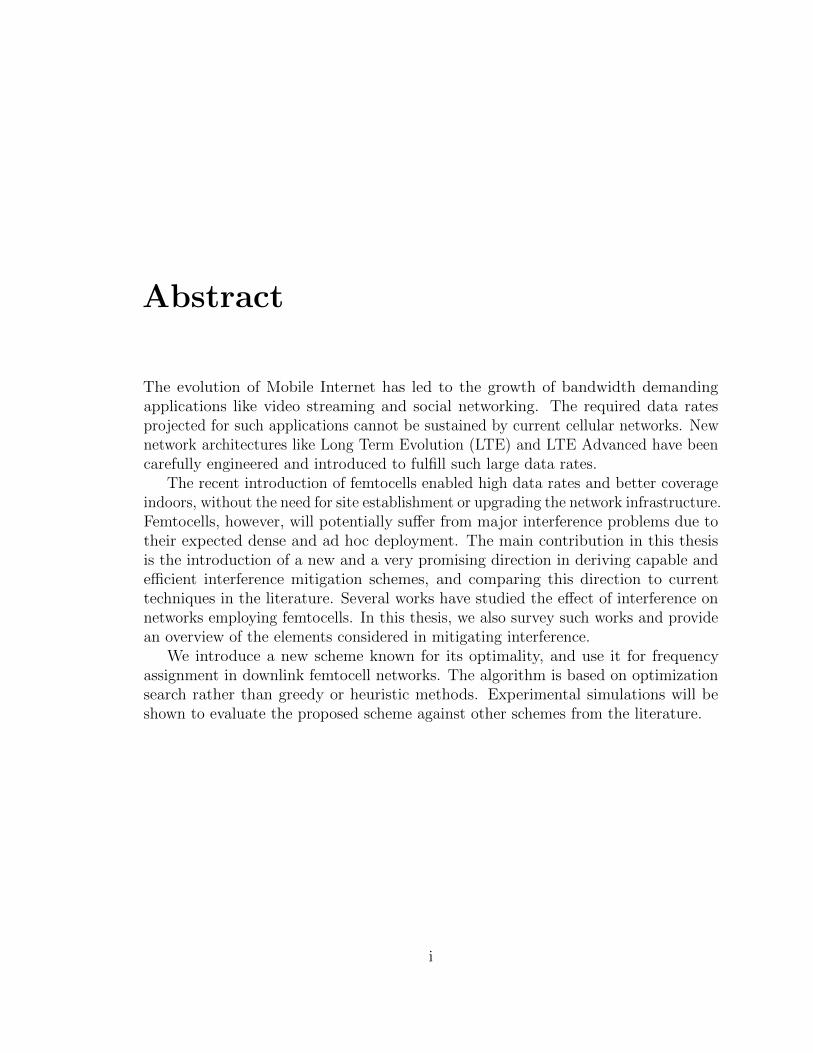
Abstract
The evolution of Mobile Internet has led to the growth of bandwidth demandingapplications like video streaming and social networking. The required data ratesprojected for such applications cannot be sustained by current cellular networks. Newnetwork architectures like Long Term Evolution (LTE) and LTE Advanced have beencarefully engineered and introduced to fulfill such large data rates.
The recent introduction of femtocells enabled high data rates and better coverageindoors, without the need for site establishment or upgrading the network infrastructure.Femtocells, however, will potentially suffer from major interference problems due totheir expected dense and ad hoc deployment. The main contribution in this thesisis the introduction of a new and a very promising direction in deriving capable andefficient interference mitigation schemes, and comparing this direction to currenttechniques in the literature. Several works have studied the effect of interference onnetworks employing femtocells. In this thesis, we also survey such works and providean overview of the elements considered in mitigating interference.
We introduce a new scheme known for its optimality, and use it for frequencyassignment in downlink femtocell networks. The algorithm is based on optimizationsearch rather than greedy or heuristic methods. Experimental simulations will beshown to evaluate the proposed scheme against other schemes from the literature.
i
Acknowledgments
The work presented in this thesis is conducted as part of the Masters program of the
School of Computing at Queen’s University, under the supervision of Dr. Hossam
Hassanein, and the co-supervision of Dr. Najah Abed AbuAli. A portion of this work
was supported by QUWIC (Qatar University Wireless Innovations Center).
I would like to thank Dr. Hossam Hassanein, from the School of Computing at
Queen’s University, for providing me with the opportunity to study at Queen’s. Dr.
Hossam have demonstrated a unique example of how a supervisor - as professional as
he was - could be a close friend. Despite being a Computer Science graduate, I have
been fit smoothly in a Telecommunications Research Lab. I knew this would have
been a challenge for Dr. Hossam and myself, but the way I was fit in this lab was just
right.
I would also like to acknowledge the efforts of Dr. Najah from the College of IT at
UAE, towards the achievement of this thesis. Dr. Najah have been co-supervising
my thesis since the early stages, and despite the time zone difference, she was able
provide guidance and she was flexibly available for clarifications.
I extend my thanks to Dr. Abd-Elhamid Taha from the School of Computing at
Queen’s University, for reviewing and providing feedback on all document artifacts
that have been used in this thesis. Dr. Taha is an example of a relentless, patient
ii

coach. I thank him for his enormous efforts and invaluable advices on the professional
and personal level.
In addition, I would convey my gratitude to my friends and family in Egypt, who
supported my decision to study abroad. Also, I would like to thank all my friends
in the Telecommunications Research Lab and School of Computing, who have been
constantly providing me with advices and whom I have spent unforgotten times with
them. I do remember people who stood beside me at the hard times, Abdulmone‘m,
Dina, Gehan, Hatem, Khalid, Layan, Mervat, Qutqut, Sharief, Shereen, and Walid.
Finally, I cannot express how much gratitude I owe my fiancee, Samar, who have
been there for me since day one. She showed extreme support throughout the duration
of my study, and was holding up really well, even at the toughest times when I was
away. Thank You!
iii
Contents
Abstract i
Acknowledgments ii
Contents iv
List of Tables vi
List of Figures vii
List of Acronyms viii
Chapter 1: Introduction 11.1 Motivation . . . . . . . . . . . . . . . . . . . . . . . . . . . . . . . . . 31.2 Problem Context . . . . . . . . . . . . . . . . . . . . . . . . . . . . . 51.3 Contribution . . . . . . . . . . . . . . . . . . . . . . . . . . . . . . . . 61.4 Thesis Organization . . . . . . . . . . . . . . . . . . . . . . . . . . . . 7
Chapter 2: Background 82.1 Indoor Coverage Techniques . . . . . . . . . . . . . . . . . . . . . . . 8
2.1.1 Repeaters . . . . . . . . . . . . . . . . . . . . . . . . . . . . . 92.1.2 Distributed Antenna Systems . . . . . . . . . . . . . . . . . . 102.1.3 Indoor Cells . . . . . . . . . . . . . . . . . . . . . . . . . . . . 102.1.4 Differences Between Femtocells and Picocells . . . . . . . . . . 11
2.2 Femtocells . . . . . . . . . . . . . . . . . . . . . . . . . . . . . . . . . 122.2.1 Nomenclature . . . . . . . . . . . . . . . . . . . . . . . . . . . 122.2.2 Femtocells features and attributes . . . . . . . . . . . . . . . . 132.2.3 Advantages of femtocells . . . . . . . . . . . . . . . . . . . . . 162.2.4 Some femtocell applications . . . . . . . . . . . . . . . . . . . 19
2.3 Channel Assignment . . . . . . . . . . . . . . . . . . . . . . . . . . . 192.4 Interference Challenge . . . . . . . . . . . . . . . . . . . . . . . . . . 21
2.4.1 Mitigating Different Interference Types . . . . . . . . . . . . . 21
iv
2.5 Interference Mitigation Solutions . . . . . . . . . . . . . . . . . . . . 222.5.1 Solutions Categorization . . . . . . . . . . . . . . . . . . . . . 24
2.6 Related Work . . . . . . . . . . . . . . . . . . . . . . . . . . . . . . . 262.6.1 Current Techniques . . . . . . . . . . . . . . . . . . . . . . . . 262.6.2 Discussion and Motivation . . . . . . . . . . . . . . . . . . . . 31
Chapter 3: Problem Formalization and Proposed Solution 343.1 System Description and Problem Definition . . . . . . . . . . . . . . 34
3.1.1 System Description . . . . . . . . . . . . . . . . . . . . . . . . 343.1.2 Problem Definition . . . . . . . . . . . . . . . . . . . . . . . . 36
3.2 Mathematical Formulation . . . . . . . . . . . . . . . . . . . . . . . . 363.3 Problem Categorization and Proposed Solution . . . . . . . . . . . . 38
3.3.1 Problem Categorization . . . . . . . . . . . . . . . . . . . . . 383.3.2 Proposed Solution . . . . . . . . . . . . . . . . . . . . . . . . 393.3.3 Minimum Cost Flow . . . . . . . . . . . . . . . . . . . . . . . 43
Chapter 4: Simulation and Performance Evaluation 514.1 Simulation Setup . . . . . . . . . . . . . . . . . . . . . . . . . . . . . 51
4.1.1 System Topology . . . . . . . . . . . . . . . . . . . . . . . . . 524.1.2 Candidate Algorithms . . . . . . . . . . . . . . . . . . . . . . 564.1.3 Kim’s Algorithm . . . . . . . . . . . . . . . . . . . . . . . . . 564.1.4 In-house Greedy Solution . . . . . . . . . . . . . . . . . . . . . 57
4.2 Simulation Results . . . . . . . . . . . . . . . . . . . . . . . . . . . . 584.2.1 Capacity Metric . . . . . . . . . . . . . . . . . . . . . . . . . . 584.2.2 Elapsed Time Metric . . . . . . . . . . . . . . . . . . . . . . . 64
4.3 Complexity and Performance Analysis . . . . . . . . . . . . . . . . . 654.4 A Note on The Achieved Results . . . . . . . . . . . . . . . . . . . . 67
Chapter 5: Summary and Conclusion 685.1 Summary . . . . . . . . . . . . . . . . . . . . . . . . . . . . . . . . . 685.2 Conclusion . . . . . . . . . . . . . . . . . . . . . . . . . . . . . . . . . 705.3 Recommendations and Future Work . . . . . . . . . . . . . . . . . . . 70
5.3.1 Fairness Issues . . . . . . . . . . . . . . . . . . . . . . . . . . . 715.3.2 Adding Support to Uplink . . . . . . . . . . . . . . . . . . . . 715.3.3 Distributed Operation . . . . . . . . . . . . . . . . . . . . . . 72
Bibliography 73
Appendix A: Derivation of SINR PDF 81
v
List of Tables
1.1 Growth of operator revenues for leading operators in Q3 2007. . . . . 5
2.1 Comparison between picocells and femtocells. . . . . . . . . . . . . . 112.2 Comparison of femtocells and other wireless devices. . . . . . . . . . . 162.3 Comparison of recent interference mitigation studies. . . . . . . . . . 33
4.1 General Simulation Parameters . . . . . . . . . . . . . . . . . . . . . 554.2 Experiment A1 specific parameters. . . . . . . . . . . . . . . . . . . . 594.3 Experiment B1 specific parameters. . . . . . . . . . . . . . . . . . . . 614.4 Experiment C1 specific parameters. . . . . . . . . . . . . . . . . . . . 634.5 Complexity analysis of the algorithms in simulation. . . . . . . . . . . 67
vi
List of Figures
1.1 Illustration of a two tiered network. . . . . . . . . . . . . . . . . . . . 31.2 Percentage of indoor to outdoor voice and data sessions. . . . . . . . 4
2.1 Comparison of conventional cell sizes. . . . . . . . . . . . . . . . . . . 122.2 Simple femtocell network. . . . . . . . . . . . . . . . . . . . . . . . . 132.3 Some key Femtocell Base Station features. . . . . . . . . . . . . . . . 152.4 Interference types in a femtocell environment. . . . . . . . . . . . . . 22
3.1 Normal Cyclic prefix OFDMA downlink Resource Block . . . . . . . 373.2 Example of a bipartite graph. . . . . . . . . . . . . . . . . . . . . . . 393.3 Example of Signal to Interference and Noise Ratio (SINR) matrix. . . 403.4 Mapping SINR matrix to a Bipartite graph. . . . . . . . . . . . . . . 403.5 Bipartite graph after adding artificial source and sink. . . . . . . . . . 413.6 A graph represented as an adjacency matrix. . . . . . . . . . . . . . . 423.7 A solved adjacency matrix. . . . . . . . . . . . . . . . . . . . . . . . . 423.8 Different data structures in a MCF problem . . . . . . . . . . . . . . 453.9 The initial network graph. . . . . . . . . . . . . . . . . . . . . . . . . 463.10 Residual network evolution. . . . . . . . . . . . . . . . . . . . . . . . 483.11 The final maximum flow network. . . . . . . . . . . . . . . . . . . . . 48
4.1 Physical layout of the simulated environment. . . . . . . . . . . . . . 534.2 Experiment A1: Average Normalized Capacity vs. changing number of
users per femtocell. . . . . . . . . . . . . . . . . . . . . . . . . . . . . 604.3 Experiment B1: Average Normalized Capacity vs. changing number of
femtocells. . . . . . . . . . . . . . . . . . . . . . . . . . . . . . . . . . 624.4 Experiment C1: Effect of applying Random Waypoint mobility model
on the normalized capacity. . . . . . . . . . . . . . . . . . . . . . . . 644.5 Experiment A2: Average Elapsed Time. . . . . . . . . . . . . . . . . 654.6 Corner case challenging the greedy approach. . . . . . . . . . . . . . . 67
vii
List of Acronyms1G First Generation
2G Second Generation
3G Third Generation
3GPP 3rd Generation Partnership Project
3GPP2 3rd Generation Partnership Project 2
4G Fourth Generation
ACI Adjacent Channel Interference
ASE Area Spectral Efficiency
BS Base Station
BSC Base Station Controller
CAPEX CAPital EXpenditure
CCI Co-Channel Interference
CDMA Code Division Multiple Access
CI Computational Intelligence
CoI Cell of Interest
CSG Closed Subscriber Group
DAS Distributed Antenna Systems
DCA Dynamic Channel Allocation
DFS Dynamic Frequency Selection
DSL Digital Subscriber Line
eNB eNode B
FAP Femtocell Access Point
FBS Femtocell Base Station
viii
FCA Fixed Channel Assignment
FFR Fractional Frequency Reuse
FUE Femtocell User Equipment
GA Genetic Algorithm
GoS Grade of Service
GPRS General Packet Radio Services
GSM Global System for Mobile Communications (Groupe Special Mobile)
HCA Hybrid Channel Allocation
HeNB Home eNode B(femtocell)
HetNet Heterogeneous Network
IEEE Institute of Electrical and Electronics Engineers
ILCA Interference Limited Coverage Area
ISI Inter-Symbol Interference
LP Linear Programming
LTE Long Term Evolution
MAC Medium Access Control
MBS Macrocell Base Station
MCF Minimum Cost Flow
MDRP Maximal Dynamic Reuse Partitioning
MUE Macrocell User Equipment
NN Neural Network
ODRP Optimal Dynamic Reuse Partitioning
OFDMA Orthogonal Frequency Division Multiple Access
OFDM Orthogonal Frequency Division Multiplexing
ix
OPEX OPerational EXpenditure
OSG Open Subscriber Group
PDF Probability Density Function
QoS Quality of Service
RB Resource Block
RRM Radio Resource Management
RSSI Received Signal Strength Indicator
RWP Random Waypoint
SA Simulated Annealing
SI Swarm Intelligence
SINR Signal to Interference and Noise Ratio
SIR Signal to Interference Ratio
SMS Short Message Service
UE User Equipment
VoIP Voice over IP
WCDMA Wideband Code Division Multiple Access
WiMAX Worldwide Interoperability for Microwave Access
x
CHAPTER 1. INTRODUCTION 1
Chapter 1
Introduction
The cellular market has always been a demanding, ever evolving market. Since the
introduction of mobile phones in the early 1990s, digital mobile phones have grown to
reach around 5 billion subscriptions worldwide, around 76% of the world population [1].
In parallel, the Internet has been also growing, to reach 1.6 billion users worldwide,
nearly 25% of the world population [2]. Blogs, social networks, video streaming and
video gaming are continuously pushing the Internet traffic to its limits.
The current cellular systems started evolving since the 1980s. The introduction
of First Generation (1G) mobile networks aimed at providing voice only services. It
was based solely on analog technologies. The 1G systems have been replaced soon by
Second Generation (2G) digital mobile systems. The primary data services introduced
in 2G were Short Message Service (SMS) and circuit-switched data services [3]. This
enabled e-mail and other data applications to rise and opened a huge amount of
market opportunities for cellular operators and application development. Post the mid
1990s, packet data has become a reality with the introduction of General Packet Radio
Services (GPRS) in Global System for Mobile Communications (GSM) networks,
CHAPTER 1. INTRODUCTION 2
referred to as 2.5G.
The introduction of Third Generation (3G) mobile services [3] has merged both
the digital mobile technology and the Internet technology. This merging boosted both
markets promoting the fact that consumers are getting too attached to their mobile
phones and increasing their hours of stay online. This also expanded the market for
new bandwidth demanding applications that encourage more mobile usage.
The current specifications of Fourth Generation (4G) wireless cellular standards
promise hundreds of Mbit/s that should reach up to 1 Gbit/s for low mobility
communications. With the ever increasing number of mobile users in the same territory,
these rates might be difficult to achieve without optimized signaling, modulation,
coding and interference resistance mechanisms. Nowadays, an emerging trend has
been put into action to virtually extend the territory covered by a certain provider,
which is: layering cellular networks, resulting in the formation of small cells within
larger cells, as in Figure 1.1. This kind of reusing the physical space, enhances what is
known as the Area Spectral Efficiency (ASE) [4, 5]. The ASE of a cellular system can
be defined as the achievable throughput per unit area for the available bandwidth [6].
Since shrinking the cell size is the simplest and most effective way of increasing wireless
throughput [7,8], hence, was the introduction of indoor base stations forming picocells
and recently femtocells [9]. The introduction of these small coverage networks requires
also optimized operational mechanisms in order to co-exist with larger macrocell
networks.
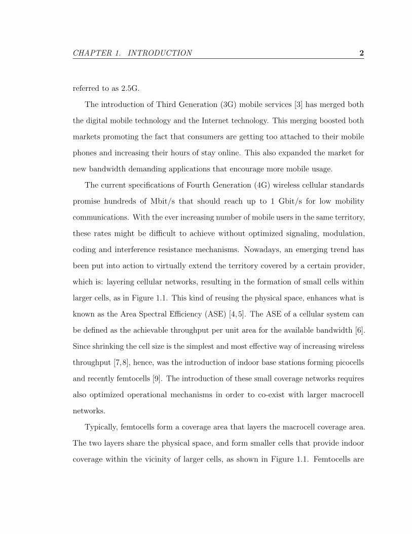
Typically, femtocells form a coverage area that layers the macrocell coverage area.
The two layers share the physical space, and form smaller cells that provide indoor
coverage within the vicinity of larger cells, as shown in Figure 1.1. Femtocells are
CHAPTER 1. INTRODUCTION 3
expected to have a very strong penetration rate at homes, offices and malls. End users
will install their Femtocell Base Stations (FBSs) on their own. FBSs installation will
be done in a convenient plug and play manner, and hence, non-coordinated ad-hoc
deployment is inevitable. Such deployment is more likely to introduce interference [10],
which will adversely affect the capacity of the radio system in addition to the quality of
the individual communication links. Capacity increase is fundamentally the result of
a trade-off between interference and quality, and hence, there is a need for interference
management techniques to minimize interference which might otherwise counteract
the capacity gains and degrade the quality of the network.
Figure 1.1: Illustration of a two tiered network, with femtocells ad-hoc deployment.
1.1 Motivation
Femtocells have been attracting much attention recently as a solution to the problem
of poor cellular indoor coverage and capacity. With the estimation that 2/3 of calls
and over 90% of data services occur indoors [9], besides, 45% of households and 30%
CHAPTER 1. INTRODUCTION 4
of businesses experience poor indoor coverage [11], the importance of indoor coverage
emerges. Providing a reliable and strong indoor coverage of voice as well as video
and high speed data services will soon be a must for mobile operators to survive. To
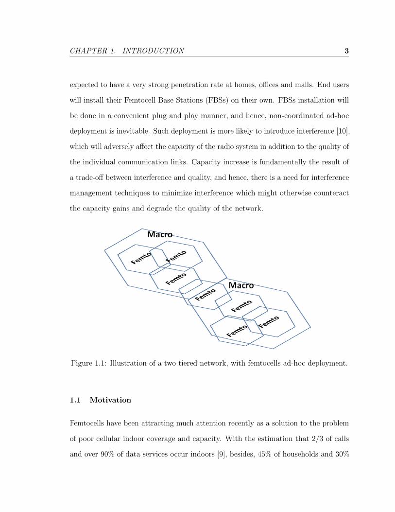
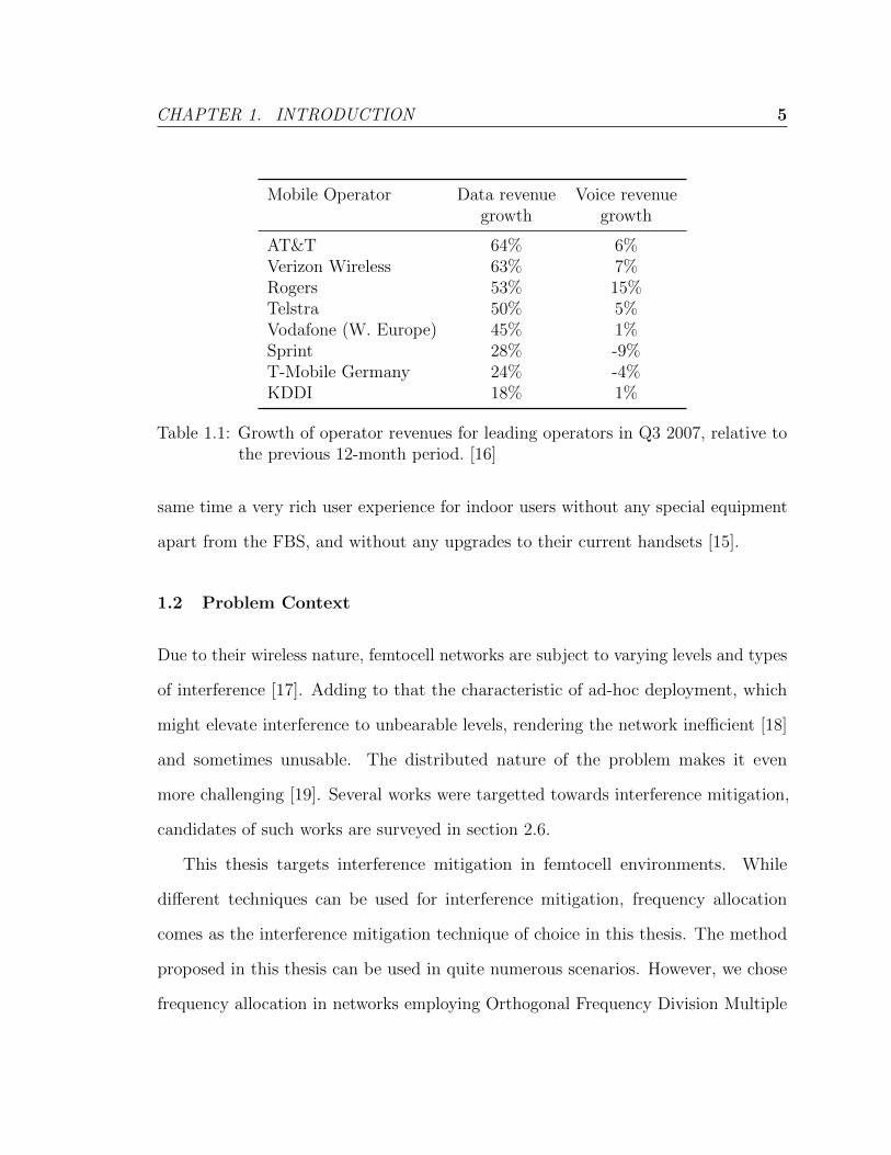
emphasize on the rising importance of data, table 1.1 shows the growth of operator
revenues for leading operators in Q3 2007, relative to the previous 12-month period,
just before the femtocell technology started to appear. It can be noticed that some
operators did not even grow positively in terms of voice revenue and that data revenue
growth was more dominant. One of the obvious reasons of the significant drop in voice
revenue is Voice over IP (VoIP) which enabled voice calls at relatively very low cost
compared to cellular operators.
Figure 1.2: Percentage of indoor to outdoor voice and data sessions. Reproducedfrom [9]
With all what preceded in mind, and given the cost of establishing a Base Station
(BS); a cheaper and more effective solution is preferred. Femtocells are expected to
substantially reduce the operator CAPital EXpenditure (CAPEX) and OPerational
EXpenditure (OPEX) [12, 13], which explains the great interest shown by cellular
operators deploying femtocells. UMTS FBSs are expected to reach 70 million devices
installed indoors, serving more than 150 million users [14], which is clearly why experts
think that femtocells represent a promising direction from the operator economic view.
Femtocells are expected to offload much traffic to indoors, freeing resources at the
macrocells and helping outdoor users to gain better user experience, providing at the
CHAPTER 1. INTRODUCTION 5
Mobile Operator Data revenuegrowth
Voice revenuegrowth
AT&T 64% 6%Verizon Wireless 63% 7%Rogers 53% 15%Telstra 50% 5%Vodafone (W. Europe) 45% 1%Sprint 28% -9%T-Mobile Germany 24% -4%KDDI 18% 1%
Table 1.1: Growth of operator revenues for leading operators in Q3 2007, relative tothe previous 12-month period. [16]
same time a very rich user experience for indoor users without any special equipment
apart from the FBS, and without any upgrades to their current handsets [15].
1.2 Problem Context
Due to their wireless nature, femtocell networks are subject to varying levels and types
of interference [17]. Adding to that the characteristic of ad-hoc deployment, which
might elevate interference to unbearable levels, rendering the network inefficient [18]
and sometimes unusable. The distributed nature of the problem makes it even
more challenging [19]. Several works were targetted towards interference mitigation,
candidates of such works are surveyed in section 2.6.
This thesis targets interference mitigation in femtocell environments. While
different techniques can be used for interference mitigation, frequency allocation
comes as the interference mitigation technique of choice in this thesis. The method
proposed in this thesis can be used in quite numerous scenarios. However, we chose
frequency allocation in networks employing Orthogonal Frequency Division Multiple
CHAPTER 1. INTRODUCTION 6
Access (OFDMA) in their downlink, as it is the multiple access scheme utilized in
emerging networks such as LTE, LTE-Advanced WiMAX.
In this thesis an optimal assignment solution is presented. It will be used as a
benchmark to other schemes from the literature. Towards the end of this thesis, the
tradeoff between performance and complexity will be discussed, and recommendations
will be presented.
One major challenge that is addressed in this thesis, is the simulation environment.
The femtocellular setup differs from the regular macrocell setup in two important
aspects: 1. The network size, and 2. The ad-hoc nature of the setup. Chapter 4
shows how simulation challenges were addressed and what assumptions have been
considered.
1.3 Contribution
The contribution in this thesis can be summarized in the following points:
1. Incorporating the SINR derivation model proposed in [20] in the modeling of a
two-tiered macrocell-femtocell environment.
2. Modeling the problem of frequency allocation to a graph theory problem and
solving it using a network flow algorithm, that finds the optimal allocation.
Optimality is defined against SINR, that is, a solution is said to be optimal
if it maximizes the summation of the overall SINR on the currently allocated
frequencies.
3. Providing a frequency allocation scheme known for its optimality, and comparing
it with other schemes, and presenting recommendations on which schemes
CHAPTER 1. INTRODUCTION 7
balances the tradeoff between complexity and performance. The proposed scheme
can be used in benchmark studies. However, this study is not a benchmark
study, rather, it involves the introduction of this scheme.
1.4 Thesis Organization
This thesis is organized as follows. Chapter 2 gives an orientation on indoor coverage
techniques that preceded femtocells. Section 2.2 provides the nomenclature and the
main feature of femtocell technology, along with its prospective applications. After-
wards, the interference challenge is presented and the current combating techniques
are summarized. Chapter 2 also surveys some of the related work in the field of
interference mitigation, and provides a comparison.
In chapter 3 the problem in study is mathematically formulated and the proposed
solution is presented in detail. Chapter 4 presents the experimental simulation done
towards the assessment of the proposed algorithm, along with the achieved results. The
chapter wraps up by a complexity and performance analysis that will aid producing
recommendations later in this thesis. Finally, chapter 5 concludes and presents future
recommendations.
CHAPTER 2. BACKGROUND 8
Chapter 2
Background
In this chapter, brief introduction to femtocell technology is presented. An overview
for the notions of channel assignment and interference is also offered. The interference
challenge and the characteristics of interference in femtocell environments are presented
in detail. Afterward, recommendations for interference mitigation solutions are
highlighted and some related works from the literature are categorized. Finally, the
essence of our proposed algorithm is revealed.
2.1 Indoor Coverage Techniques
Indoor coverage is traditionally achieved via macrocell signalling. Radio planning
rules, such as link budget and transmission power, control the level of indoor coverage.
Operators try to maintain an acceptable level of ‘economic’ indoor coverage, that
is, satisfying indoor user, hence generating revenue, without much investment in the
establishing of macrocells. Nowadays, users expect more reliable and larger capacity
communication. Increasing the number of macrocells or transmission power is limited
CHAPTER 2. BACKGROUND 9
by budgetary or interference constraints. This is when enhanced indoor coverage
becomes a challenge to cellular operators. Due to the importance of indoor coverage
and the significant percentage of indoor sessions (data or voice), several techniques
have been developed to target this issue [2,9]. This section explains some representative
techniques.
2.1.1 Repeaters
Since outdoor signals attenuate heavily at the walls of buildings; an intuitive idea is
to have a component that amplifies these raw signals so they can reach indoor User
Equipments (UEs) at acceptable power levels. Such a component is called a repeater,
and can be one of two types:
Passive repeaters. They amplify signals in a certain frequency band, regardless of
their nature. A passive repeater consists of:
1. An external antenna, placed outside a building, pointing to the nearest
outdoor antenna sector.
2. An amplifier, to strengthen the signal by amplification, usually leads to a
gain of 30-50 dB.
3. An indoor antenna, to redistribute the signal. Directional or omni-directional
antennas are typical candidates.
Active repeaters. Are more sophisticated than passive repeaters. They are capable
of decoding and reshaping the signal before retransmitting it.
The choice of repeaters is based on the tradeoff between technology and cost. The
cheaper passive repeaters can be used in places when the only required enhancement
CHAPTER 2. BACKGROUND 10
is signal amplification. While active repeaters can be used in confined areas where
much errors are expected, because they can increase the data rate by decreasing the
data transmission errors that may occur. On the other hand, passive repeaters are not
advised in high error rate environments because when using higher frequencies, the
degradation of the signal can greatly affect the quality of the transmission. Proposal
that combine both types of repeaters already exist [21].
2.1.2 Distributed Antenna Systems
Distributed Antenna Systems (DAS) [22] are based on the idea of replacing an antenna
transmitting at high power with a number of smaller antennas transmitting at lower
powers. A number of components can be used to split the signal power between the
small antennas. For example, coaxial cables, splitters, taps, attenuators and filters.
Like repeaters, DAS can be passive or active. The reader is encouraged to review
chapter 2 from [9] for more information about DAS.
2.1.3 Indoor Cells
Prior to the success of WiFi, operators started to consider extending mobile networks
via a clever concept; which is having smaller cells that provide good coverage to a
specific set of users in an area. This emerged Picocells. These new picocells rely
on small BSs that use lower power levels and, thus, less capacity compared to the
outdoor BSs serving the larger macrocells. A picocell is connected to the core network
via standard in-building wiring, fibre optic or Ethernet connections. It connects to an
operator Base Station Controller (BSC), which manages the tasks of data transmission
between the picocell and the network, performs handover between the cells, and
CHAPTER 2. BACKGROUND 11
manages resource allocation to different users.
Femtocells are more different than picocells. More of residential/private/home
owned base stations. A femtocell is connected to the operator network directly via the
Internet. Femtocells are limited in power and capacity. The classical models of home
femtocells demonstrated an output power between 10 to 20 dBm, and supported a
number of users between 3 to 5.
2.1.4 Differences Between Femtocells and Picocells
This section provides insight on the differences between femtocells and related tech-
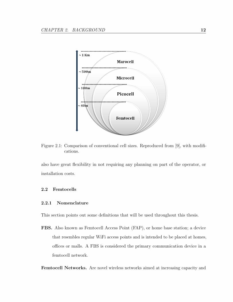
nologies. Table 2.1 summarizes the differences between picocells and femtocells. Figure
2.1 shows a comparison between conventional cell sizes.
Criterium Picocell Femtocell
Installation By the operator By the end userConnection to the core network Coaxial or fibre optic ADSL or cableCapacity 10-50 users 3-5 usersCoverage 100m-200m < 50m1
1 For typical home femtocells. Longer range femtocells will be available forlarger facilities such as malls and offices.
Table 2.1: Comparison between picocells and femtocells. Reproduced from [9], withmodifications.
Picocells rely on the operator network infrastructure. Thus, their positions need
to be planned. Femtocells, on the other hand, connect to the core via any Internet
connection that allows for the relevant authentication procedures to take place. The
operator therefore saves the cost of the additional infrastructure required. They
CHAPTER 2. BACKGROUND 12
Figure 2.1: Comparison of conventional cell sizes. Reproduced from [9], with modifi-cations.
also have great flexibility in not requiring any planning on part of the operator, or
installation costs.
2.2 Femtocells
2.2.1 Nomenclature
This section points out some definitions that will be used throughout this thesis.
FBS. Also known as Femtocell Access Point (FAP), or home base station; a device
that resembles regular WiFi access points and is intended to be placed at homes,
offices or malls. A FBS is considered the primary communication device in a
femtocell network.
Femtocell Networks. Are novel wireless networks aimed at increasing capacity and
CHAPTER 2. BACKGROUND 13
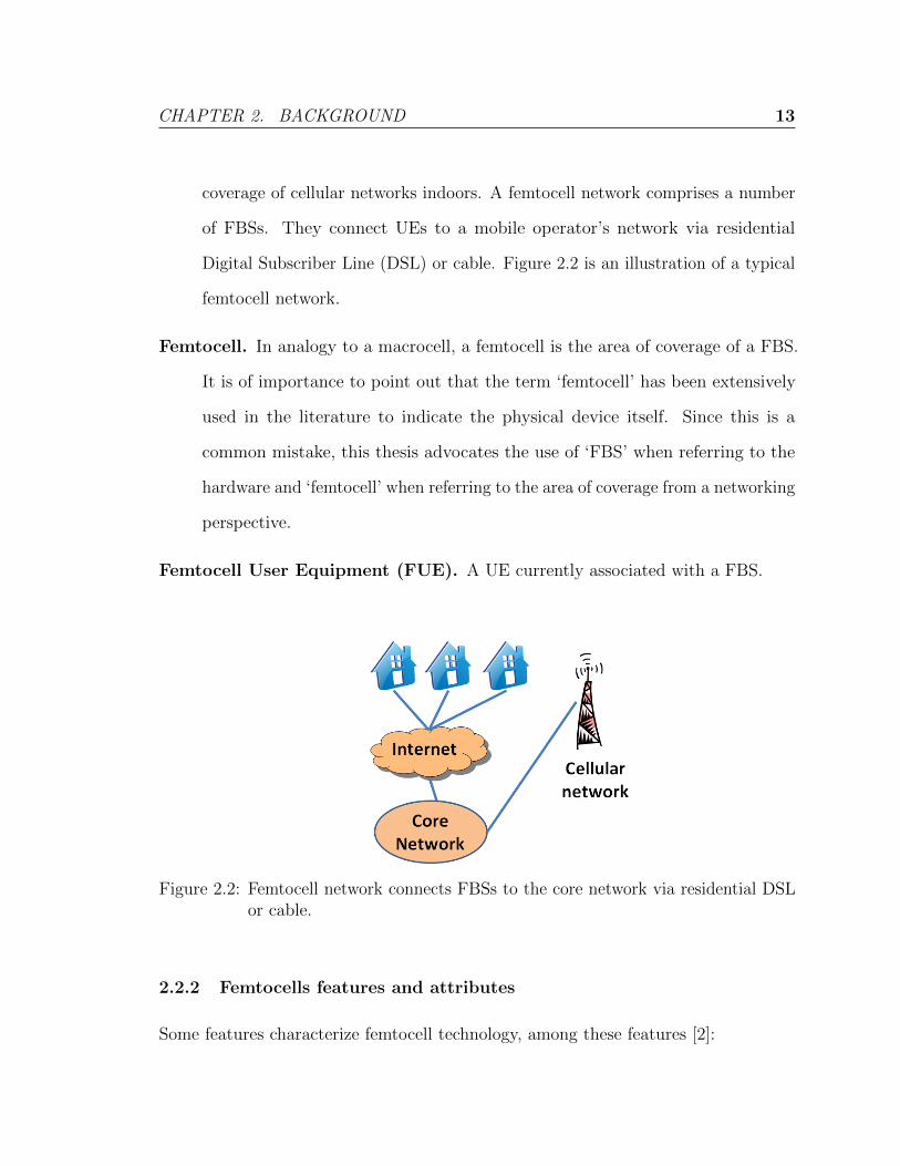
coverage of cellular networks indoors. A femtocell network comprises a number
of FBSs. They connect UEs to a mobile operator’s network via residential
Digital Subscriber Line (DSL) or cable. Figure 2.2 is an illustration of a typical
femtocell network.
Femtocell. In analogy to a macrocell, a femtocell is the area of coverage of a FBS.
It is of importance to point out that the term ‘femtocell’ has been extensively
used in the literature to indicate the physical device itself. Since this is a
common mistake, this thesis advocates the use of ‘FBS’ when referring to the
hardware and ‘femtocell’ when referring to the area of coverage from a networking
perspective.
Femtocell User Equipment (FUE). A UE currently associated with a FBS.
Figure 2.2: Femtocell network connects FBSs to the core network via residential DSLor cable.
2.2.2 Femtocells features and attributes
Some features characterize femtocell technology, among these features [2]:
CHAPTER 2. BACKGROUND 14
Usage of mobile technology. Femtocell technology targets complementing the cur-
rent cellular systems. Hence, it is assumed to integrate with the readily available
cellular components including mobile phones and cellular protocols and interfaces.
Qualifying standard protocols include GSM, WCDMA, LTE, Mobile WiMAX,
CDMA, as well as current and - supposedly - future protocols standardized by
3GPP, 3GPP2 and the IEEE/WiMAX forum.
Operation in licensed spectrum. This allows supporting regular mobile devices
without the need of dual-mode devices to use in a femtocell.
Coverage and capacity enhancement. FBSs transmit in relatively very low power
targeting a very small indoor area compared to Macrocell Base Stations (MBSs).
The very short distance between a transmitter and a receiver promotes the use
of higher order modulation schemes and hence promotes higher capacity [22, 23].
Backhauled to the cellular network. Data sent from a FBS is backhauled to the
cellular network through DSL or cable, using standard Internet protocols.
Zero-touch feature. FBSs will support plug n’ play [24]. This feature mandates
that a user should have no involvement in either installing or operating the home
device save for powering it on. The initial configuration, re-configuration and
the rest of the device operation should be seamless to the user and should not
entail any technical support. Although the FBSs will receive their operation
parameters via the operator network, this operation will be done automatically
under the hood, without any user intervention.
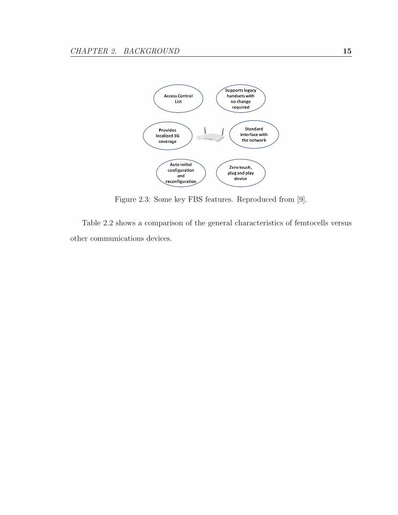
Figure 2.3 shows the main features of a FBS.
CHAPTER 2. BACKGROUND 15
Figure 2.3: Some key FBS features. Reproduced from [9].
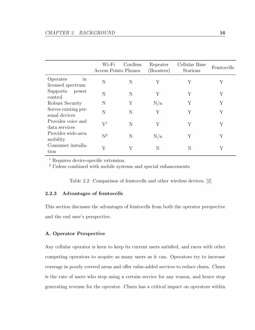
Table 2.2 shows a comparison of the general characteristics of femtocells versus
other communications devices.
CHAPTER 2. BACKGROUND 16
Wi-FiAccess Points
CordlessPhones
Repeater(Boosters)
Cellular BaseStations
Femtocells
Operates inlicensed spectrum
N N Y Y Y
Supports powercontrol
N N Y Y Y
Robust Security N Y N/a Y YServes existing per-sonal devices
N N Y Y Y
Provides voice anddata services
Y1 N Y Y Y
Provides wide-areamobility
N2 N N/a Y Y
Consumer installa-tion
Y Y N N Y
1 Requires device-specific extension.2 Unless combined with mobile systems and special enhancements
Table 2.2: Comparison of femtocells and other wireless devices. [2]
2.2.3 Advantages of femtocells
This section discusses the advantages of femtocells from both the operator perspective
and the end user’s perspective.
A. Operator Perspective
Any cellular operator is keen to keep its current users satisfied, and races with other
competing operators to acquire as many users as it can. Operators try to increase
coverage in poorly covered areas and offer value-added services to reduce churn. Churn
is the rate of users who stop using a certain service for any reason, and hence stop
generating revenue for the operator. Churn has a critical impact on operators within
CHAPTER 2. BACKGROUND 17
a competitive environment. This section discusses the benefit of employing femtocells
to the operator.
Increase system coverage and capacity. By offloading indoor connections to a
femtocell instead of a macrocell. This frees up resources on the macrocell to
service more outdoor users. Also, this increases the capacity of indoor users by
connecting them to near indoor FBSs.
Filling coverage holes. A MBS adjusts its transmission power to serve as many
users as it can. However, the tradeoff between power and interference is resolved
by limiting transmission power to a certain level, which results in the creation of
‘pockets’ or ‘holes’ between macrocells. Unfortunate users who reside within these
holes experience very low signal level, lower than what may be required to make
a call. Femtocells fit perfectly in situations like this. Minimal interference from
macrocells due to their poor signals will hardly affect the femtocell performance,
and at the same time, femtocells will cover a large portion of the gaps.
Reduce churn. Churn represents a considerable loss to operators specially in sat-
urated markets. The value of a current customer increases when less or no
other potential customers are out there. Poor indoor coverage can cause churn,
however, with the introduction of femtocells, value-added family packages can
be delivered to the customer, and hence, reducing churn to a great extent.
Cutting costs. By increasing the system capacity without the need for new cell sites
for macrocells, the operator will experience huge savings in terms of CAPEX
and OPEX [2,9, 12,13,25].
CHAPTER 2. BACKGROUND 18
B. End User’s Perspective
Subscribers rush towards better quality services, lower prices, or unique services that
are not offered by other operators. While most users are not ready to pay the extra
dollar for current services, operators try to convince users with new services in order
to increase their revenues. This section presents forms of attraction that femtocells
can offer to subscribers.
Better service. In addition to enhanced coverage and capacity stated before, fem-
tocells will also help the operator provide richer services like femtozone-based
services, and bundled services, and other bandwidth consuming applications,
which will also encourage mobile usage indoors [25].
Cheaper prices. By installing new base stations inside homes, that will also be
maintained later by the end user; operators can offer value-added services like
free or cheap calls from home or free ‘inside-office’ calls.
Centralized management. Femtocells can offer a single address book and one
billing account for both land line phone, broadband and mobile phone.
Saving power. Because of the short distance between a FBS and a UE; battery
operated devices will communicate using lower power levels than those required
to communicate to a macrocell, resulting in longer battery life. This will also
reduce health concerns on using mobile devices.
Femtocell nature will attract consumers for a number of reasons. For instance,
femtocells will not require users to have dual-mode devices which will relief the worry
of purchasing new devices that are compatible with femtocells. Also, the fact that
CHAPTER 2. BACKGROUND 19
femtocells will be available in Closed Subscriber Group (CSG) mode gives consumers
a sense of security and privacy.
2.2.4 Some femtocell applications [9]
Femtozone services. Services based on the presence of mobile devices within the
coverage area of a home femtocell. For example, the FBS can send an SMS
when a user enters the femtozone, or synchronize pictures and videos from a
trip [25]. Another promising application can be a ‘virtual number’ to reach
all people currently in the house, or for holding conference calls with family
members. Enterprise VoIP [26], and file transfer [27] can also be categorized as
femtozone services.
Connected home services. Home automation applications and controlling home
equipments via mobile phones are good examples of connected home services
that are expected to spread with the introduction of femtocells.
2.3 Channel Assignment
Channel assignment is the process of assigning bandwidth to BSs to be split later
among UEs. Bandwidth is needed to transmit signals modulated with data. Channel
assignment, frequency allocation, frequency scheduling; these definitions have been
used interchangeably in the literature to indicate the process of assigning frequency
slots to terminals to transmit data over them. The quality of an assignment is governed
by many factors:
Complexity. Less complex frequency allocation is more favored than complicated
procedures. In advanced network architectures, the rate by which the frequency
CHAPTER 2. BACKGROUND 20
allocation can occur is as high as once every 10ms.
Bandwidth fragments. Some channel allocation schemes uses fixed allocations,
which may cause bandwidth fragments, and decrease the utilization of bandwidth.
SINR. Is a measure of how good a link between a BS and a UE. Changing the
allocated channel(s) affects the resulting SINR.
In short three types of channel allocation strategy exist [28]:
Fixed Channel Assignment (FCA). Is a technique where a pre-computed fixed
set of channels is assigned to a cell. The channel sets are computed to be less
vulnerable to Co-Channel Interference (CCI). However, this scheme might cause
sessions in crowded cells to be rejected when resource admission cannot be
granted.
Dynamic Channel Allocation (DCA). Is a technique where channels are allo-
cated ‘on-demand’ as cells request them for transmission. This technique is
considered more resource-aware but renders the system more interference vulner-
able. Thus, requires more calculations and real-time data on channel occupancy,
traffic distribution and Received Signal Strength Indicator (RSSI).
Hybrid Channel Allocation (HCA). Uses both FCA and DCA in conjunction.
The process involves FCA for some resources then DCA for the rest. As per [28]
This technique has been adopted by some fairly old studies like [29–31]. It can
also been seen from the modern literature that studies concerned with HCA are
still on track [32].
CHAPTER 2. BACKGROUND 21
2.4 Interference Challenge
Generally, interference occurs when two or more devices are transmitting ‘near’ each
other. The definition involves devices that are either physically near each other, or
devices transmitting on near frequencies or channels. As is well known, the wireless
medium faces many types of interference. For example, Inter-Symbol Interference (ISI),
which occurs when a symbol overlaps with following symbols due to the delayed multi-
path signal. Co-Channel Interference (CCI) occurs when a device transmits on the same
channel being used by a nearby device. Whereas Adjacent Channel Interference (ACI)
happens when signals from a device transmitting on a certain channel interfere with
signals of another device on another channel.
FBSs are meant to be installed indoors to cover relatively very small areas compared
to traditional macrocells. Unless deployed in very remote areas, femtocells will always
be overlaid on macrocells, rendering such deployments as a two-tiered, composed of
a macro-tier and a femto-tier. This tiered deployment is vulnerable to cross-layer
interference [9,10,17], which is the type of interference that occurs between cells of
different types, e.g., Femto-to-Macro or Macro-to-Femto. In addition to cross-layer
interference, co-layer interference might occur between two cells within the same layer
See Figure 2.4 for a simple illustration of interference types in a femtocell environment.
2.4.1 Mitigating Different Interference Types
Cross-layer interference can be greatly reduced by a setup through which the available
spectrum is partitioned between the macrocellular and the femtocellular layers. This
setup, however, limits the amount of spectrum available for each layer and is considered
CHAPTER 2. BACKGROUND 22
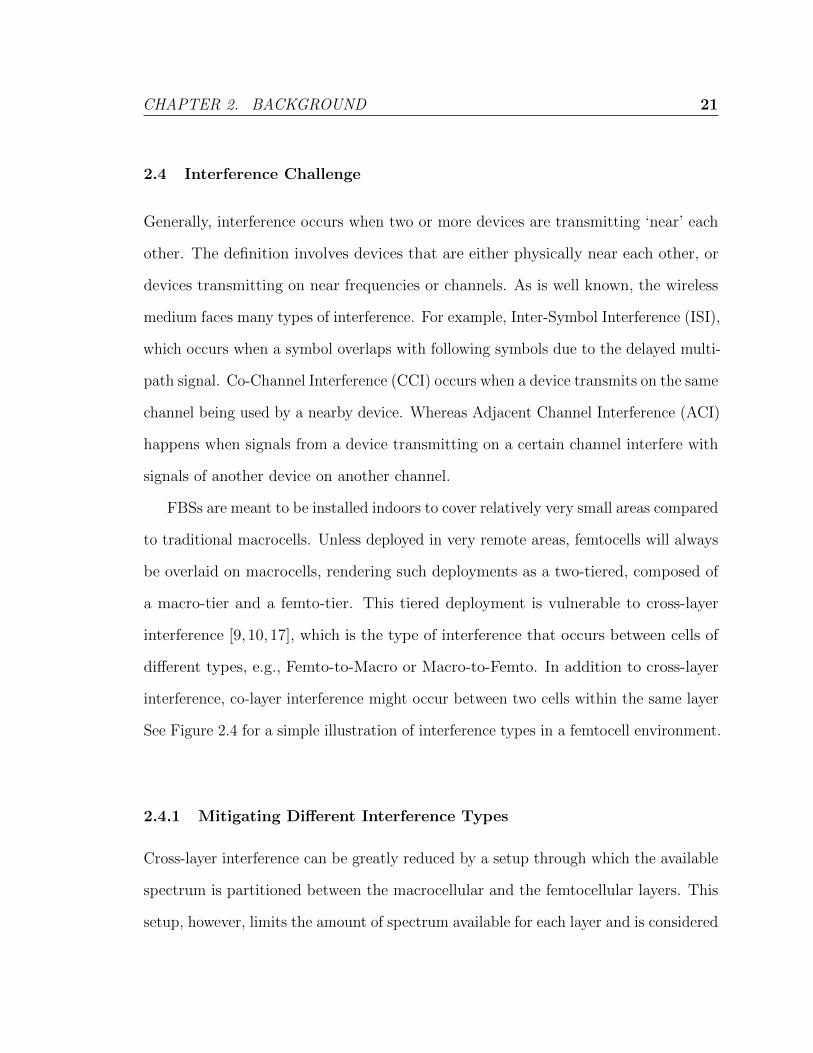
Figure 2.4: Interference types in a femtocell environment: the dashed line showsco-layer interference and the solid line shows cross layer interference
less efficient [6]. On the other hand the whole spectrum or part of it can be shared
between the two layers resulting in larger system capacity, but rendering the system
more interference vulnerable. In [33] the authors proposed a hybrid spectrum sharing
technique, trying to achieve a lower interference and a high capacity system at the
same time. Conversely, co-layer interference can be mitigated to a great extent using
proper frequency allocation and scheduling techniques, or dynamic power adjustment.
In this chapter, representatives of the different techniques that have been devised
to mitigate different interference types will be discussed. Section 2.6 presents the
result of a literature survey that was conducted for this purpose.
2.5 Interference Mitigation Solutions
Innovative interference mitigation techniques should be used with this novel type of so-
phisticated networks. Proposals to mitigate interference should take into consideration
the nature of femtocells for a number of reasons:
1. Femtocells operate in licensed spectrum.
CHAPTER 2. BACKGROUND 23
2. FBSs are installed and maintained by end users.
3. FBSs have limited computation and signalling power compared to regular outdoor
BSs.
4. Femtocells are in most cases overlaid on macrocells
Using these facts, we can derive a number of parameters that should be considered
when designing femtocell interference mitigation solutions to ensure applicability:
Complexity requirements. Unlike the regular MBSs, the initial objective of a FBS
is to provide better indoor voice and data services in a simple and cost effective
way. This results in a small size FBS with limited computation and processing
power. However, deployment issues necessitate avoiding complex algorithms
for the mitigation purposes. By surveying the literature, we speculate that
optimized algorithms based on Computational Intelligence (CI) like Genetic
Algorithms (GAs), Simulated Annealing (SA), Neural Networks (NNs) and
Game Theoritic-based algorithms will gain momentum in the context of research
to provide stronger solutions.
Distributed Operation. In order to minimize decision delay, it is important that
localized decisions are made, foregoing centralized processing, and the delays
required for the two-way signalling.
Adaptability. Distributivity is often linked to adaptability. Interference mitigation
algorithms are expected to be highly adaptable to the surrounding environment
since new FBSs can be deployed anywhere at anytime which will keep the current
network infrastructure topology in a state of continuous change compared to
the ordinary cellular network.
CHAPTER 2. BACKGROUND 24
Scalability. The projected density of deployment for femtocells also necessitates
scalable solutions. To appreciate the minimal scale of deployment, the installation
of a FBS per household should be assumed. This projected enormous volume
entails highly scalable solutions.
One important aspect that should be also regarded is self-organization [34,35]. The
aforementioned zero-touch feature [24] mandates that a FBS be able to do self-
configuration, self-optimization, and self-healing [9, 18]. The self-configuration charac-
teristic mandates that a device, once powered up, starts collecting its configuration
parameter and does configuration tasks, whether these parameters are hard-coded,
on-chip, or reside on some server. On the other hand, self-optimization ensures that
the device is always in a state of optimizing parameters such as signalling, power
and frequency allocation to guarantee calm and effective communication. Finally,
self-healing states that if certain communication failure or degrading happens, the
device should find fixes and apply them to continue operation. Self-organization is
composed of all three, and is needed to ensure that the FBS unit can function on its
own. Self-organization has been proposed at different phases of femtocell standard-
ization. It can also be linked to adaptability because a FBS is in a continuous state
of operation optimization. Signalling, power level and computations are examples of
what can be optimized whilst the operation of a FBS.
2.5.1 Solutions Categorization
Interference mitigation solutions can be categorized against a number of criteria:
Operator managed vs FBS vendor managed. An operator managed solution
affirms that the cellular provider coordinates the work of different femtocells and
CHAPTER 2. BACKGROUND 25
supplies them with parameters for operating interference mitigation solutions;
whereas a FBS vendor managed (on-chip) solution requires that FBSs ship
pre-configured with certain interference mitigation out-of-the-box mechanisms
regardless of the network they will be deployed as part of.
Locality. A localized solution runs at each femtocell, without the need for central
coordination of calculations between FBSs. Localized techniques are more
preferable to support scalability which requires that a FBS works on its own or
in rare cases communicates with the surrounding FBSs. Conversely, network-
wide techniques provide acceptable operation with generally less sophistication
because they depend on specific central entities that aggregate information from
groups of femtocells and use this information to compute solutions. Local versus
network-wide solutions are also referred to as decentralized versus centralized
solutions.
Application level. Categorization per application level describes the level of granu-
larity at which the solution is applied, i.e., at the tier level or at the cell level.
Solutions deployed at the coarse grained tier level tend to use durable, less or
no changing parameters. In contrast, fine grained cell level solutions work on a
much lower level and they need to be more adaptable and highly configurable.
An example to show the difference between tier level and cell level is frequency
planning in opposition to frequency allocation. In a multi-tier environment
portions of the spectrum is split among tiers, without going deeper to cells;
this is a tier-level technique. On the other hand, frequency allocation, where
users within a cell are admitted frequency slots for transmission, is considered a
cell-level technique.
CHAPTER 2. BACKGROUND 26
2.6 Related Work
2.6.1 Current Techniques
Recently, many studies have been proposing interference mitigation techniques accord-
ing to different environment setups and different scenarios. The resulting solutions
range from basic optimizations to sophisticated powerful solutions. The latter ones
are less dependent on physical and Medium Access Control (MAC) layers and are
more efficient in terms of signalling, but at the cost of intensive computations. In
what follows, we summarize these different techniques.
Frequency planning. Interference can be mitigated at the planning stage as it is
possible, for example, to split the available spectrum into bands among cells
within a cellular system to minimize intercell interference, i.e., interference that
occurs within adjacent cells when UEs on the edge of cells receive mixed signals.
Spectrum splitting. In multi-tier networks, operators use spectrum splitting to
dedicate portions of the spectrum to different tiers. Some solutions support high
level of sharing between tiers, resulting in a higher capacity but more interference
vulnerable systems. Meanwhile, other solutions can be based on total spectrum
separation between layers which provide greater resistance to interference but at
the cost of lowering the system capacity. Hybrid systems were also proposed,
e.g. in [33], to define a solution based on the trade-off between interference and
capacity. Spectrum splitting is used mainly to combat cross-layer interference.
Power control. Is a solution applied at the cell level. It aims at adjusting the
transmission power of BSs to limit unnecessary high power that might cause
interference with the surrounding cells, or affect near transmissions.
CHAPTER 2. BACKGROUND 27
Frequency allocation. Is another cell level solution aiming at combating interference
by proper allocation of frequency channels to users. Subcarrier allocation, which
has been recently adopted with new access technologies, such as OFDMA, has
been studied thoroughly as an effective way of combating interference. Fractional
Frequency Reuse (FFR) [36,37], Dynamic FFR [38], and Dynamic Frequency
Selection (DFS) algorithms [39] have been proposed in this matter.
More recently, different studies have addressed interference mitigation. The fol-
lowing paragraphs shed the light on candidate interference mitigation solutions to
familiarize the reader with the state of the art related studies from the literature.
In [40], the authors advocate the importance of distributed, self-optimizing schemes
due to the fact that locations and the number of FBSs exploit a high level of uncer-
tainty. The authors solve an optimization problem to control the overall transmission
power of FBSs in a femtocell OFDMA network, subject to individual rate and power
constraints. According to the authors, an optimal solution requires information about
all communication links, and this kind of information is not readily available at all
times. So, the authors propose a distributed power control and scheduling algorithm
as explained in the next paragraph.
Each user has a Quality of Service (QoS) constraint in the form of a threshold
SINR for a given service; the objective is to meet the required SINR at each user.
The problem is modeled as a Linear Programming (LP) problem and is solved using
Particle Swarm Optimization, an example of a Swarm Intelligence (SI) approach. SI
exhibits the communal behavior of self-organizing entities in a distributed environment.
Many of the techniques categorized as SI approaches are copied from nature, such as
ant colonies and animal herding. The proposed algorithm yields sub-optimal solutions
CHAPTER 2. BACKGROUND 28
on each femtocell and in the event that no feasible solution exists, a heuristic sacrificial
mechanism is employed to defer some transmissions of users causing high interference
based on the users’ nominal SINR. The algorithm is based on heuristics and takes
into account the femtocellular layer only and involves alot of signalling, but in favor
of being decentralized.
In [28], the authors suggest two reuse partitioning schemes to be applied on
overlaid - multiple layered - networks. The main idea involves adapting cluster size to
maintain high Signal to Interference Ratio (SIR), and applying channel assignment.
Each hexagonal cell can be viewed as a set of concentric hexagonal cells, each with a
different radius.
Two schemes were proposed: 1. Maximal Dynamic Reuse Partitioning (MDRP),
and 2. Optimal Dynamic Reuse Partitioning (ODRP). In MDRP, excess channels
are assigned to the innermost region in order to acquire maximum effective capacity
from the subject cell. Alternatively, in ODRP, the system allocates unused channels
in line with the areas and the distribution of users within the concentric SIR regions,
in order to maintain a certain Grade of Service (GoS). The adaptive nature of the
proposed schemes makes them more powerful than similar schemes.
In [41], the authors study mitigating downlink Femto-to-Macro interference through
dynamic resource partitioning. The system under study is an OFDMA two tiered
network that employs universal frequency reuse. Since the transmission power of
eNode Bs (eNBs) is much more than that of Home eNode Bs (HeNBs), then it is likely
that Macrocell User Equipments (MUEs) within the transmission range of femtocells
will cause interference to the UEs around, and will itself experience low SINR. To
preserve universal frequency reuse, the authors suggested prohibiting HeNBs from
CHAPTER 2. BACKGROUND 29
accessing downlink resources that are assigned to near MUEs. By doing so, interference
to the most vulnerable MUEs - as per the authors - is effectively controlled at the
cost of sacrificing minor portion of the femtocell capacity. The study is based on
the assumption that giving up some femtocell resources will lead to a better system
throughput. The authors defended this assumption in their study.
In [42], the authors propose a greedy based dynamic frequency assignment scheme.
The core idea of the scheme is to assign the quietest channels to femtocells according
to the received power level. The algorithm is two-fold: 1. Each FBS scans the
entire spectrum and selects the frequency bandwidth that shows the lowest received
power level, and 2. Each FBS measures then sorts the received power level on every
sub-channel of its frequency bandwidth and assigns the quietest sub-channels to its
UEs. The algorithm may not yield powerful results compared to similar algorithms
in the field, but is considered fast and not complex, especially that it works in a
decentralized manner.
In [43], the authors exploit coverage adaptation through balancing FBSs transmis-
sion powers. Power control decisions are made according to the available mobility
information about the surrounding users. And the goal is not to leak much pilot
signal outside a house, which may lead to increasing mobility events, or decrease the
power too much, which may also cause the same problem. The study is considered
a contribution to the auto-configuration and self-optimization aspects in femtocell
networks. The paper distinguishes between auto-configuration and self-optimization
in the sense that auto-configuration is responsible for initially configuring the FBS,
whereas the self-optimization is concerned with enhancing the current configuration
during operation.
CHAPTER 2. BACKGROUND 30
Auto power configuration is proposed via three different approaches:
Fixed power. All FBSs start transmission with a fixed power. This is considered the
easiest approach of all, but clearly it can be enhanced with simple calculations
as depicted in the two other approaches.
Distance based. A FBS starts transmission with a power value such that the sur-
rounding UEs receive this power as strong as the power received from the
macrocell. This way, unnecessary mobility events can avoided to a great extent.
The macrocell power is estimated using a path-loss model.
Measurement based. Works as distance based, but the difference is that the macro-
cell power is not estimated, rather is measured by the FBS. This requires a
built-in measuring capability in the FBS.
After auto-configuration, self-optimization comes into play. The proposed self-
optimization approaches aim at minimizing the number of mobility events.
In [32], the authors assume a two-tier (femto-macro) environment, and present
the capacity-interference tradeoff resulting from using shared bandwidth versus using
dedicated bandwidth. The proposed idea is splitting the area around a macrocell
into inner and outer regions. A FBS within the inner region will not operate in a
co-channel mode (shared bandwidth) to avoid interference, rather it uses a frequency
band other than that used by the MBS. The authors tackled the calculation of the
best threshold the splits the inner and outer regions. Interference Limited Coverage
Area (ILCA) is derived via estimating power levels using different path-loss models.
In [44], the authors study the effects of two power control schemes namely geo-
static power control and adaptive power control. In geo-static power control, the
CHAPTER 2. BACKGROUND 31
transmission power of a femtocell is based on its distance from the macrocell. However,
in adaptive power control, the transmission powers of femtocells are adjusted based
on the network target rates, enhancing the femtocell users’ throughput without much
degradation in the macrocell performance.
In [45], the authors use a non-cooperative game theoretic approach to model the
distributed power control of femtocells, where each FBS is a player trying to decide
its transmission power whilst maximizing its benefit. The system considers fairness in
its model too; femtocells serving more mobile stations should be allowed to transmit
at higher power levels to maintain service to its users. A payoff function based on
revenue and cost was derived, where the cost is directly proportion to the transmission
power, to advise FBSs to reduce their transmission powers. Transmission powers reach
Nash Equilibrium (steady state) in the simulated game. Game theory has been also
used in other femtocell interference mitigation related studies [46,47].
In [12], the authors study a centralized Radio Resource Management (RRM) for
femtocell dense deployment. They derive an objective function to maximize the system
capacity. The problem is divided to two sub-problems: 1. sub-channel allocation,
and 2. Power allocation. In [48] the authors advocate the idea of preventing some
frequencies from being used by a femtocell if they are already assigned to a near MUE.
Availability of macrocell frequency scheduling information is assumed.
2.6.2 Discussion and Motivation
We studied the recommended characteristics of future interference mitigation solutions.
Based on the comparison from the literature presented in this thesis, we can infer
that there is still a large void when it comes to optimized solutions. We have been
CHAPTER 2. BACKGROUND 32
studying the applicability of a centralized frequency allocation algorithm, that makes
use of graph theory and optimization. The addition to what is currently offered in
the literature is seeding the optimization. We focus on using optimal assignment
algorithms rather than random or greedy based assignments. This should boost the
performance of our technique when we devise a decentralized version of it. We take
into consideration the fact that femtocells are overlaid on macrocells, so we incorporate
both layers in the algorithm dynamics. We also take into account the trade-off between
complexity and performance, to produce a high quality applicable solution that we
believe it will assist in filling the gap in the current interference mitigation solutions.
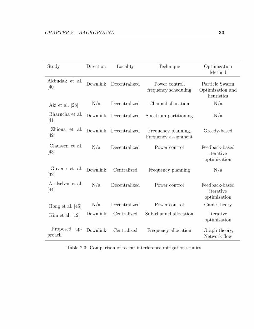
Table 2.3 shows a comparison between recent studies from the literature. Last
entry in this table is our proposed solution.
In the next chapter, we are proposing a novel approach that models the spectrum
allocation problem as an assignment problem, and solves it using a graph theoretic
approach in an efficient and optimal way. The solution is based on a popular net-
work flow solution, namely the Minimum Cost Flow (MCF) algorithm. A resulting
assignment is considered optimal if the summation of SINRs of the assigned RBs is
maximized. The proposed solution runs in a centralized manner, so it is assumed
that there will be a central entity to gather information from BSs and manage the
algorithm running to find the best possible frequency assignment to all users within a
macrocell and the overlaid femtocells.
CHAPTER 2. BACKGROUND 33
Study Direction Locality Technique OptimizationMethod
Akbudak et al.[40]
Downlink Decentralized Power control,frequency scheduling
Particle SwarmOptimization and
heuristics
Aki et al. [28] N/a Decentralized Channel allocation N/a
Bharucha et al.[41]
Downlink Decentralized Spectrum partitioning N/a
Zhioua et al.[42]
Downlink Decentralized Frequency planning,Frequency assignment
Greedy-based
Claussen et al.[43]
N/a Decentralized Power control Feedback-basediterative
optimization
Guvenc et al.[32]
Downlink Centralized Frequency planning N/a
Arulselvan et al.[44]
N/a Decentralized Power control Feedback-basediterative
optimization
Hong et al. [45] N/a Decentralized Power control Game theory
Kim et al. [12] Downlink Centralized Sub-channel allocation Iterativeoptimization
Proposed ap-proach
Downlink Centralized Frequency allocation Graph theory,Network flow
Table 2.3: Comparison of recent interference mitigation studies.
CHAPTER 3. PROBLEM FORMALIZATION AND PROPOSED SOLUTION 34
Chapter 3
Problem Formalization and
Proposed Solution
This chapter describes the problem context in detail, in terms of technologies and
infrastructure assumed. It also discusses how resources are requested and assigned.
Moreover, it describes the nature of the problem in study, modeling it to an assignment
problem, and solving it using graph theory. The proposed solution reduces the
assignment problem to a network flow problem, and solves it using MCF algorithm.
3.1 System Description and Problem Definition
3.1.1 System Description
This study is concerned with downlink interference mitigation by proper frequency
allocation in OFDMA networks. Mixed OFDMA networks comprising femto-tiers
layering macro-tiers are considered. The preceding statements can be broken down
into a set of characteristics that describes the environment upon which the proposed
CHAPTER 3. PROBLEM FORMALIZATION AND PROPOSED SOLUTION 35
scheme should be run:
OFDMA System. As the air interface technology of choice for downlink in LTE,
OFDMA is considered in simulation.
Downlink. The study focuses on downlink direction instead of both, downlink and
uplink directions. Specialty in this matter allowed for the development of a
tailored powerful algorithm.
Tiered Deployment Model. Practicality mandates that the proposed algorithm
supports tiered deployment, where femtocells layer macrocells. Simulating such
deployment as it seems a bit harder, is closer to the reality, and this will create
a more practical scheme than many other schemes in this area.
High Level Operation
In an OFDMA system with mixed BSs - (FBSs and MBSs) - one possible spectrum
management scheme is using shared spectrum, instead of dedicated spectrum, also
known as co-channel operation, where the bandwidth is shared between the macrocellu-
lar and the femtocellular layers. Each BS has a finite number of Resource Blocks (RBs)
representing the available spectrum, and has a number of UEs uniformly distributed
within the cell radius. At each BS, downlink SINR is calculated as presented in [20].
For each femtocell, a matrix is created, composed as the arrangement of the calculated
SINR values, where a row represents SINR values for a specific UE per each RB. A
centralized entity aggregates all matrices generated at all BSs to compose one matrix
of all UEs against RBs. MCF algorithm is then run on this matrix to produce an
optimal solution in terms of maximizing the total SINR.
CHAPTER 3. PROBLEM FORMALIZATION AND PROPOSED SOLUTION 36
3.1.2 Problem Definition
Consider the aforementioned OFDMA network with two layers, a femtocellular layer
within a macrocellular layer. The macrocellular layer is the traditional layer in the
cellular network which encompasses MBSs deployed at specific cell sites, whereas the
femtocellular layer consists of several shorter range cells resulting from the deployment
of FBSs in an ad-hoc manner. Each BS has a number of UEs to serve. UEs that belong
to the femtocellular layer, i.e., connected to FBSs, are referred to as Femtocell User
Equipments (FUEs), whereas UEs connected to a MBS are referred to as Macrocell
User Equipments (MUEs). UEs are served in units of RBs. In OFDMA downlink,
a RB is a basic time-frequency unit (see Figure 3.1), it consists of 12 consecutive
subcarriers in the frequency domain and 7 OFDM symbols in the time domain,
assuming normal cyclic prefix.
The minimum unit to serve a UE is a RB, that is, a user is either admitted access
to a whole RB or not. The problem investigated in this study is the assignment of
resource blocks among system users. An optimal assignment algorithm is proposed,
aimed at maximizing the system capacity.
3.2 Mathematical Formulation
Given L mixed - femto and macro - BSs labeled 1 through L, let Uj be the number
of UEs associated with BS j, where 1 ≤ j ≤ L. For each cell one can measure the
SINR for each UE per each RB. This can be arranged in a matrix SUj ,R where R is
the number of RBs in the accessible spectrum. Each entry in this matrix signifies the
SINR that a UE will experience when assigned a specific RB.
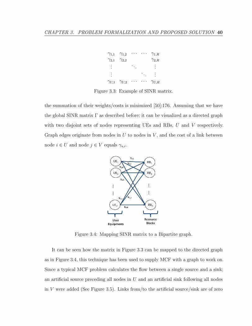
All resulting SINR matrices of all BSs are aggregated into one matrix ΓU,R by
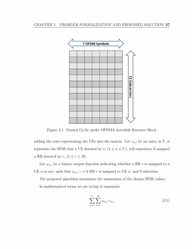
CHAPTER 3. PROBLEM FORMALIZATION AND PROPOSED SOLUTION 37
Figure 3.1: Normal Cyclic prefix OFDMA downlink Resource Block
adding the rows representing the UEs into the matrix. Let γu,r be an entry in Γ, it
represents the SINR that a UE denoted by u, (1 ≤ u ≤ U), will experience if assigned
a RB denoted by r, (1 ≤ r ≤ R).
Let ωu,r be a binary output function indicating whether a RB r is assigned to a
UE u or not, such that ωu,r = 1 if RB r is assigned to UE u, and 0 otherwise.
The proposed algorithm maximizes the summation of the chosen SINR values.
In mathematical terms we are trying to maximize:
U∑u=1
R∑r=1
ωu,r.γu,r (3.1)
CHAPTER 3. PROBLEM FORMALIZATION AND PROPOSED SOLUTION 38
Subject to constraint: ∑∀u
ωu,r ∈ {0, 1} (3.2)
The objective function in expression 3.1 indicates that the summation of SINR of all
assigned RBs is to be maximized, while the only constraint in expression 3.2 means
that a RB will be assigned to at most one UE.
3.3 Problem Categorization and Proposed Solution
3.3.1 Problem Categorization
The problem falls under the category of Assignment Problems. In general, assignment
is a combinatorial optimization, that involves assigning or ‘matching’ elements to
other elements in a manner that a satisfies a set of criteria. Any assignment problem
can be visualized as a graph G(N,E), where N is a list of nodes - or vertices - and E
is a list of edges that connects between graph vertices.
The specific problem of assigning RBs to UEs can be modeled as a Transportation
Problem [49]. In a Transportation Problem a set of graph nodes N is partitioned into
two subsets U and V (not necessarily of equal cardinality) such that:
1. Each node in U is a supply node.
2. Each node in V is a demand node.
3. A set of edges running between the two subsets exist. Each edge (i, j) joins a
node i ∈ U with a node j ∈ V
The classical example of this problem is the distribution of goods from warehouses
to customers. In this example, warehouses are represented by nodes in U and customer
CHAPTER 3. PROBLEM FORMALIZATION AND PROPOSED SOLUTION 39
zones are represented by nodes in V . An edge (i, j) represents a distribution channel
from warehouse i to customer j. Usually a cost function is associated with each edge
to indicate the incurred cost of using this edge in a solution.
Note that since the two subsets U and V are disjoint. Accordingly, the ordering
of sets does not matter, and edges that run between subsets can still be modeled as
directed edges. To make the implementation easier, the proposed solution uses this
kind of modeling variation, so it is worth mentioning here. In the proposed solution U
represents the demand nodes and V represents the supply nodes, a link (i, j) means a
node i is supplied via node j.
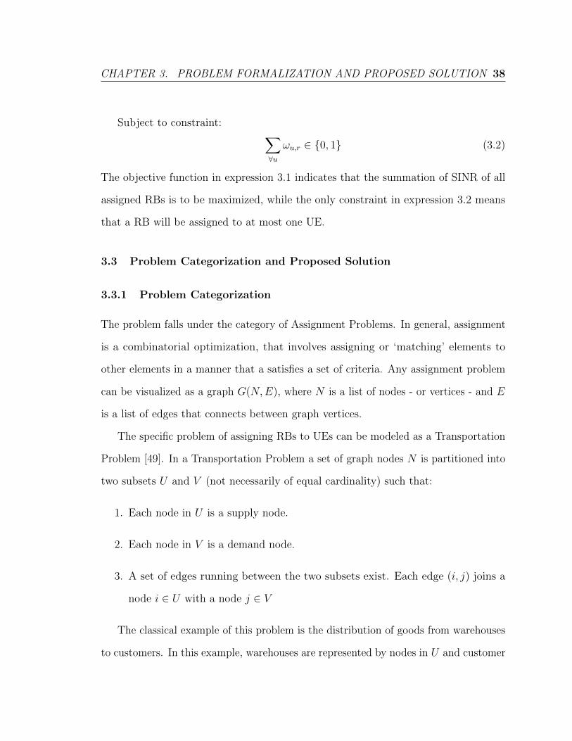
The generic modeling of this problem is a bipartite graph (see figure 3.2), with
two disjoint sets U and V .
Figure 3.2: Example of a bipartite graph.
3.3.2 Proposed Solution
MCF is known to give the optimal solution to a network visualized as a directed
weighted graph, and this optimal solution represents a set of edges chosen such that
CHAPTER 3. PROBLEM FORMALIZATION AND PROPOSED SOLUTION 40
γ1,1 γ1,2 · · · · · · γ1,R
γ2,1 γ2,2 γ2,R...
. . ....
.... . .
...γU,1 γU,2 · · · · · · γU,R
Figure 3.3: Example of SINR matrix.
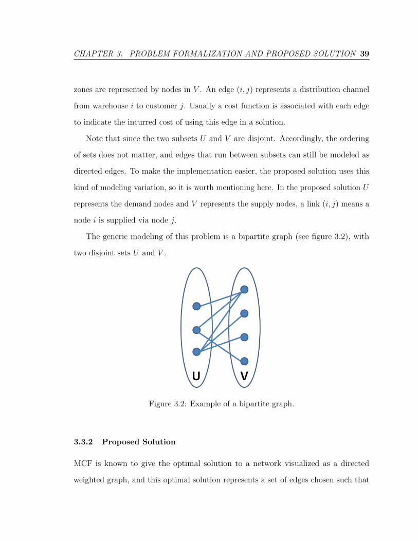
the summation of their weights/costs is minimized [50]:176. Assuming that we have
the global SINR matrix Γ as described before; it can be visualized as a directed graph
with two disjoint sets of nodes representing UEs and RBs, U and V respectively.
Graph edges originate from nodes in U to nodes in V , and the cost of a link between
node i ∈ U and node j ∈ V equals γu,r.
Figure 3.4: Mapping SINR matrix to a Bipartite graph.
It can be seen how the matrix in Figure 3.3 can be mapped to the directed graph
as in Figure 3.4, this technique has been used to supply MCF with a graph to work on.
Since a typical MCF problem calculates the flow between a single source and a sink;
an artificial source preceding all nodes in U and an artificial sink following all nodes
in V were added (See Figure 3.5). Links from/to the artificial source/sink are of zero
CHAPTER 3. PROBLEM FORMALIZATION AND PROPOSED SOLUTION 41
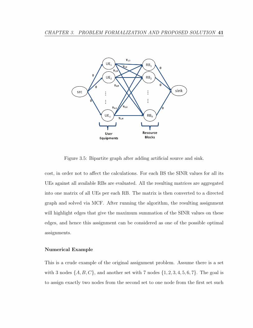
Figure 3.5: Bipartite graph after adding artificial source and sink.
cost, in order not to affect the calculations. For each BS the SINR values for all its
UEs against all available RBs are evaluated. All the resulting matrices are aggregated
into one matrix of all UEs per each RB. The matrix is then converted to a directed
graph and solved via MCF. After running the algorithm, the resulting assignment
will highlight edges that give the maximum summation of the SINR values on these
edges, and hence this assignment can be considered as one of the possible optimal
assignments.
Numerical Example
This is a crude example of the original assignment problem. Assume there is a set
with 3 nodes {A,B,C}, and another set with 7 nodes {1, 2, 3, 4, 5, 6, 7}. The goal is
to assign exactly two nodes from the second set to one node from the first set such
CHAPTER 3. PROBLEM FORMALIZATION AND PROPOSED SOLUTION 42
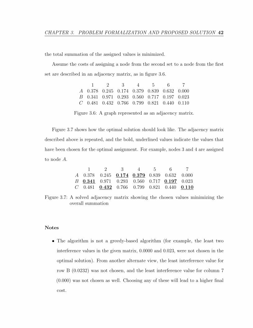
the total summation of the assigned values is minimized.
Assume the costs of assigning a node from the second set to a node from the first
set are described in an adjacency matrix, as in figure 3.6.
1 2 3 4 5 6 7A 0.378 0.245 0.174 0.379 0.839 0.632 0.000B 0.341 0.971 0.293 0.560 0.717 0.197 0.023C 0.481 0.432 0.766 0.799 0.821 0.440 0.110
Figure 3.6: A graph represented as an adjacency matrix.
Figure 3.7 shows how the optimal solution should look like. The adjacency matrix
described above is repeated, and the bold, underlined values indicate the values that
have been chosen for the optimal assignment. For example, nodes 3 and 4 are assigned
to node A.
1 2 3 4 5 6 7A 0.378 0.245 0.174 0.379 0.839 0.632 0.000B 0.341 0.971 0.293 0.560 0.717 0.197 0.023C 0.481 0.432 0.766 0.799 0.821 0.440 0.110
Figure 3.7: A solved adjacency matrix showing the chosen values minimizing theoverall summation
Notes
• The algorithm is not a greedy-based algorithm (for example, the least two
interference values in the given matrix, 0.0000 and 0.023, were not chosen in the
optimal solution). From another alternate view, the least interference value for
row B (0.0232) was not chosen, and the least interference value for column 7
(0.000) was not chosen as well. Choosing any of these will lead to a higher final
cost.

CHAPTER 3. PROBLEM FORMALIZATION AND PROPOSED SOLUTION 43
• The resulting summation (1.633) is the absolute lowest value of all solutions
that can be achieved given the problem constraints (2 nodes from the second
set should be associated to a node from the first set), that is, the algorithm is
designed to find the optimal solution.
3.3.3 Minimum Cost Flow
Description of a Flow Problem
A flow problem can be visualized as a set of connected pipes with different sizes
(referred to as: capacities, which is the maximum number of flow units that can flow
through a pipe), and the goal of the problem is to find a maximum flow of water for
instance, from the start/source of this network to the end/sink of it. This maximum
flow is bounded by the capacities of pipes; within each different path from source to
sink, the maximum flow in a path will be capped by the minimum flow among all
tubes on this path.
A MCF problem adds a new constraint to the original problem other than the pipes
capacities, namely the cost. The flow of water in a pipe is subject to a certain cost
that is predefined to this pipe. So while maximizing the anticipated flow through the
network, the cost of this flow is minimized, and this is why the problem is sometimes
called: Minimum Cost Maximum Flow.
What is a Maximum Flow?
A final maximum flow always satisfy the following:
• The total flow through the network is summation of the assigned flows on the
edges leaving the source, or alternatively entering the sink.
CHAPTER 3. PROBLEM FORMALIZATION AND PROPOSED SOLUTION 44
• A flow on an edge is always less than or equal to the capacity of this edge.
• The sum of aggregated flows leaving a vertex equals to the sum of aggregated
flows entering it.
• This sum is maximal.
In addition to a maximum flow solution, a minimum cost solution satisfies that this
maximum flow considers the minimum cost applicable.
Graph Representation in a MCF Problem
This section is essential if the reader is planning to read Example 3.3.3.
Vertex. Is a node in the graph where:
• vertex.distance is the shortest distance so far from the source node to the current
node (in terms of cost). In other words, it keeps track of the minimum cost
incurred to reach this vertex from the source.
• vertex.flow is the amount of units flowing through this node.
• vertex.parent is the immediate predecessor of this node.
Edge. Is a directed link between two nodes/vertices where:
• edge.start: is the node where this link originates from.
• edge.end: is the node where this link is directed to.
• edge.capacity is the number of flow units that can flow through this edge.
• edge.cost is the distance traveled through this edge from start to end.
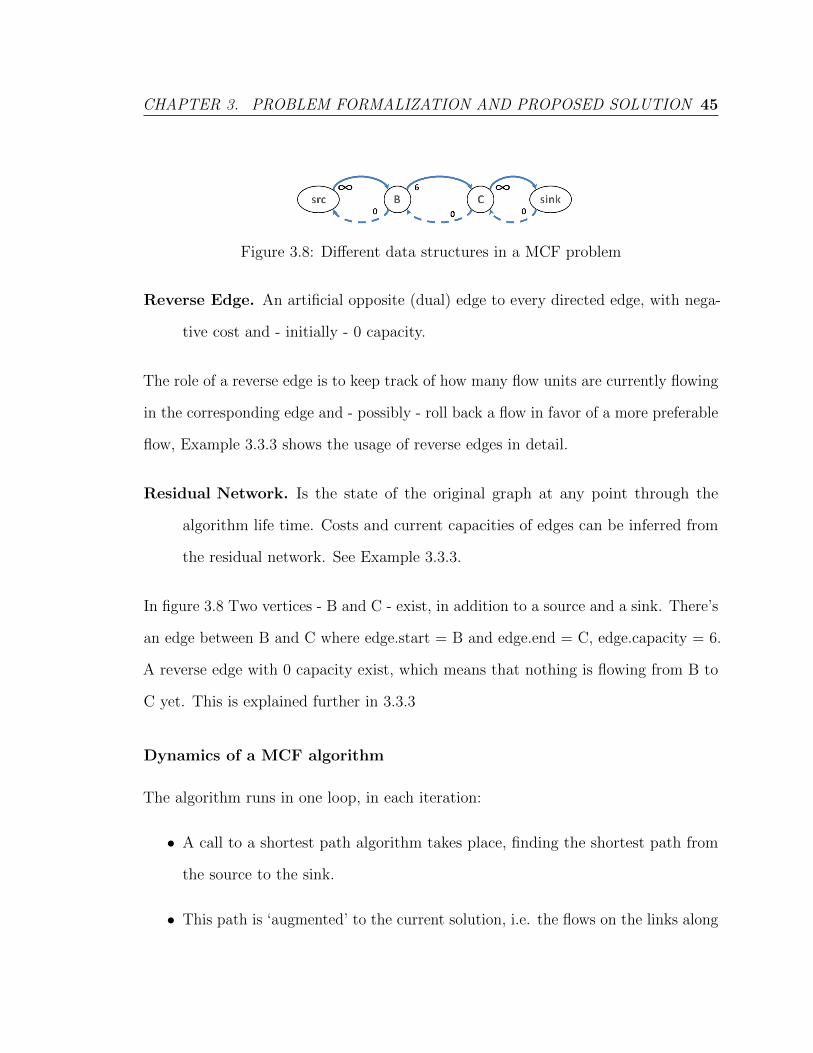
CHAPTER 3. PROBLEM FORMALIZATION AND PROPOSED SOLUTION 45
Figure 3.8: Different data structures in a MCF problem
Reverse Edge. An artificial opposite (dual) edge to every directed edge, with nega-
tive cost and - initially - 0 capacity.
The role of a reverse edge is to keep track of how many flow units are currently flowing
in the corresponding edge and - possibly - roll back a flow in favor of a more preferable
flow, Example 3.3.3 shows the usage of reverse edges in detail.
Residual Network. Is the state of the original graph at any point through the
algorithm life time. Costs and current capacities of edges can be inferred from
the residual network. See Example 3.3.3.
In figure 3.8 Two vertices - B and C - exist, in addition to a source and a sink. There’s
an edge between B and C where edge.start = B and edge.end = C, edge.capacity = 6.
A reverse edge with 0 capacity exist, which means that nothing is flowing from B to
C yet. This is explained further in 3.3.3
Dynamics of a MCF algorithm
The algorithm runs in one loop, in each iteration:
• A call to a shortest path algorithm takes place, finding the shortest path from
the source to the sink.
• This path is ‘augmented’ to the current solution, i.e. the flows on the links along
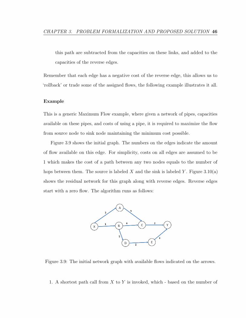
CHAPTER 3. PROBLEM FORMALIZATION AND PROPOSED SOLUTION 46
this path are subtracted from the capacities on these links, and added to the
capacities of the reverse edges.
Remember that each edge has a negative cost of the reverse edge, this allows us to
‘rollback’ or trade some of the assigned flows, the following example illustrates it all.
Example
This is a generic Maximum Flow example, where given a network of pipes, capacities
available on these pipes, and costs of using a pipe, it is required to maximize the flow
from source node to sink node maintaining the minimum cost possible.
Figure 3.9 shows the initial graph. The numbers on the edges indicate the amount
of flow available on this edge. For simplicity, costs on all edges are assumed to be
1 which makes the cost of a path between any two nodes equals to the number of
hops between them. The source is labeled X and the sink is labeled Y . Figure 3.10(a)
shows the residual network for this graph along with reverse edges. Reverse edges
start with a zero flow. The algorithm runs as follows:
Figure 3.9: The initial network graph with available flows indicated on the arrows.
1. A shortest path call from X to Y is invoked, which - based on the number of

CHAPTER 3. PROBLEM FORMALIZATION AND PROPOSED SOLUTION 47
hops - should yield to either X − A− C − Y or X −B − C − Y . Assuming the
latter was chosen, all edges along this path will have their flows decreased by
the minimum flow observed on this path which is 1, whereas reverse edges will
have their flows increased by 1. As a result of this step the flow between X and
B will be 0 and hence X −B will not be considered when qualifying another
shortest path between X and Y . Figure 3.10(b) show the residual network after
this step.
2. The next call to a shortest path yields X − A− C − Y , decreasing all flows
along this path by 2 and adding 2 to the corresponding reverse edges, Figure
3.10(c) show the residual network after this step.
3. One more call to a shortest path yields X − A− C −B −D − E − Y , with an
extra flow of 1. Note that since there was a flow from C to B it was considered
when calculating the shortest path. Having C −B in the shortest path means
that the 1 flow unit that was flowing through B − C to reach Y before will flow
in the path B −D − E − Y instead, also one of the flow units that were flowing
in C − Y will instead come from the path X − A− C.
4. A subsequent call to a shortest path from X to Y will yield no more paths. The
final residual network is shown in figure 3.10(d) and the final flow network is
shown in figure 3.11.
Below is a pseudo-code for the max flow algorithm that solves an assignment
problem.
Pseudo-code
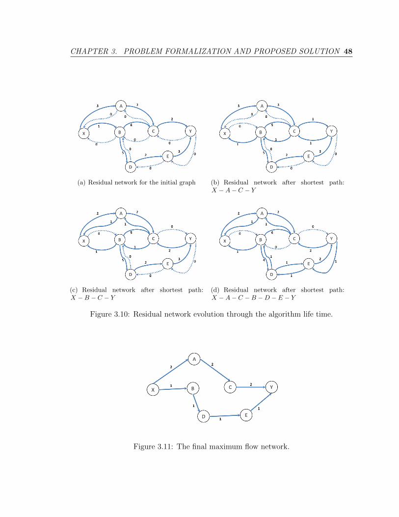
CHAPTER 3. PROBLEM FORMALIZATION AND PROPOSED SOLUTION 48
(a) Residual network for the initial graph (b) Residual network after shortest path:X −A− C − Y
(c) Residual network after shortest path:X −B − C − Y
(d) Residual network after shortest path:X −A− C −B −D − E − Y
Figure 3.10: Residual network evolution through the algorithm life time.
Figure 3.11: The final maximum flow network.
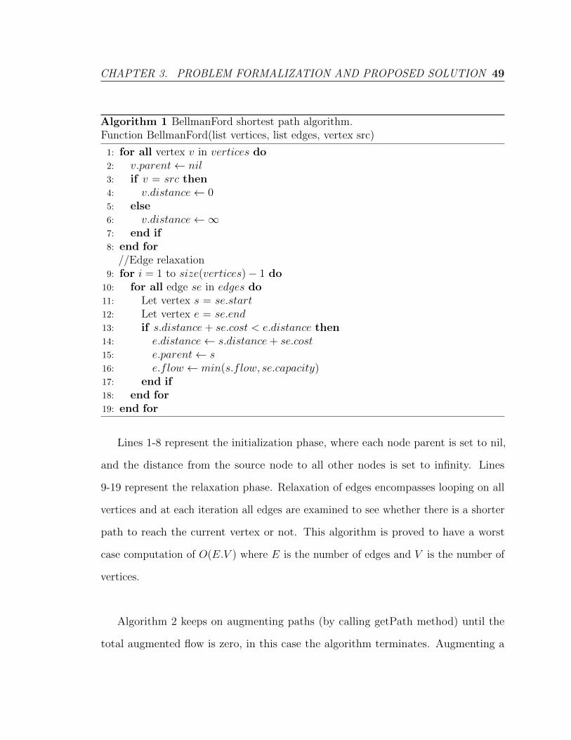
CHAPTER 3. PROBLEM FORMALIZATION AND PROPOSED SOLUTION 49
Algorithm 1 BellmanFord shortest path algorithm.Function BellmanFord(list vertices, list edges, vertex src)
1: for all vertex v in vertices do2: v.parent← nil3: if v = src then4: v.distance← 05: else6: v.distance←∞7: end if8: end for
//Edge relaxation9: for i = 1 to size(vertices)− 1 do10: for all edge se in edges do11: Let vertex s = se.start12: Let vertex e = se.end13: if s.distance+ se.cost < e.distance then14: e.distance← s.distance+ se.cost15: e.parent← s16: e.flow ← min(s.flow, se.capacity)17: end if18: end for19: end for
Lines 1-8 represent the initialization phase, where each node parent is set to nil,
and the distance from the source node to all other nodes is set to infinity. Lines
9-19 represent the relaxation phase. Relaxation of edges encompasses looping on all
vertices and at each iteration all edges are examined to see whether there is a shorter
path to reach the current vertex or not. This algorithm is proved to have a worst
case computation of O(E.V ) where E is the number of edges and V is the number of
vertices.
Algorithm 2 keeps on augmenting paths (by calling getPath method) until the
total augmented flow is zero, in this case the algorithm terminates. Augmenting a

CHAPTER 3. PROBLEM FORMALIZATION AND PROPOSED SOLUTION 50
Algorithm 2 Minimum Cost Maximum Flow algorithm.
1: while true do2: getPath(vertices, edges, source) {Call Bellmanford shortest path}3: pathflow ← dest.f low4: if pathflow = 0 then5: return6: end if7: current← sink8: while current 6= source do9: se.capacity ← se.capacity − pathflow {let se be the directed edge from
current.parent to current}10: rev.capacity ← rev.capacity + pathflow {let rev be the reverse edge of se}11: current← current.parent12: end while13: end while
path subtracts a number of flow units from all edges on this path and add the same
number of flow units to the reverse path, this helps doing reroutes as necessary, and
prevents the algorithm from recalculating an already established path.
CHAPTER 4. SIMULATION AND PERFORMANCE EVALUATION 51
Chapter 4
Simulation and Performance
Evaluation
This chapter describes the software simulation and experimental work that have been
done to assess the performance of the proposed solution. This chapter presents the
simulation environment setup such as supported system architecture, physical network
layout, frequency planning model and SINR generation model. Simulation assumptions
and general simulation parameters are mentioned in detail. Evaluation metrics and
their respective simulation scenarios are also presented, along with scenario specific
parameters. Simulation results and complexity analysis are shown towards the end of
this chapter.
4.1 Simulation Setup
We built an in-house Java® based framework to simulate the different evaluation
scenarios. We chose to develop an in-house simulator because at the time of this
CHAPTER 4. SIMULATION AND PERFORMANCE EVALUATION 52
decision, the available popular simulators like OPNET and NS-2 did not have available
simulation modules for indoor small cells such as femtocells. We have chosen to
develop our simulator using an industrial programming language because it supports
high level of flexibility for writing, debugging and maintaining code. The simulation
framework was built following a pluggable architecture, so that new algorithms can
be added for comparison following simple steps.
4.1.1 System Topology
System Architecture
The system under simulation is an OFDMA network, composed of two tiers, namely
macro-tier and femto-tier. The macro-tier encompasses a sole macrocell and a number
of macrocell users, referred to as Macrocell User Equipments (MUEs). Whereas the
femto-tier consists of a number of femtocells and their respective users. Femtocell
users are referred to as Femtocell User Equipments (FUEs).
Physical Layout
Figure 4.1 shows the network layout of the simulated environment. The layout of the
simulated network consists of:
• One FBS, referred to as: center femtocell, is placed at the origin.
• The MBS is placed at some distance North to the center femtocell.
• A number of FBSs are placed around the center femtocell in a random fashion.
• For each MBS or FBS, a number of UEs are randomly generated around the BS.
An exception to this is the MBS, where users are generated in the direction of
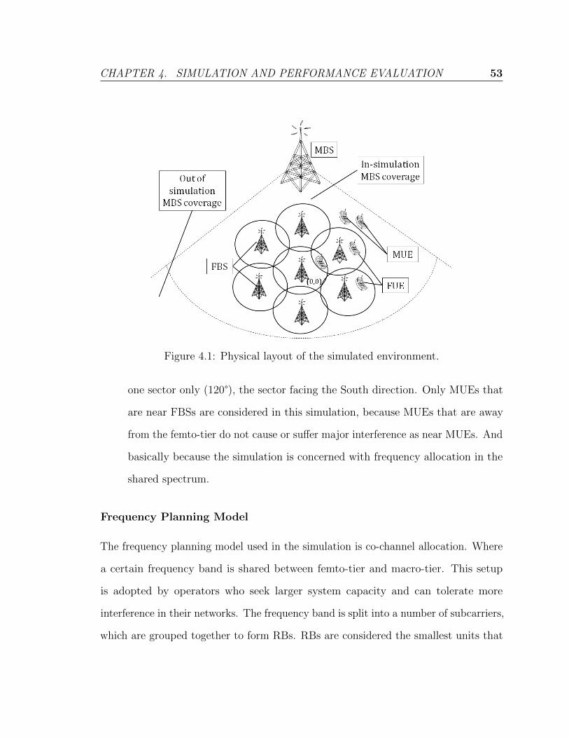
CHAPTER 4. SIMULATION AND PERFORMANCE EVALUATION 53
Figure 4.1: Physical layout of the simulated environment.
one sector only (120°), the sector facing the South direction. Only MUEs that
are near FBSs are considered in this simulation, because MUEs that are away
from the femto-tier do not cause or suffer major interference as near MUEs. And
basically because the simulation is concerned with frequency allocation in the
shared spectrum.
Frequency Planning Model
The frequency planning model used in the simulation is co-channel allocation. Where
a certain frequency band is shared between femto-tier and macro-tier. This setup
is adopted by operators who seek larger system capacity and can tolerate more
interference in their networks. The frequency band is split into a number of subcarriers,
which are grouped together to form RBs. RBs are considered the smallest units that
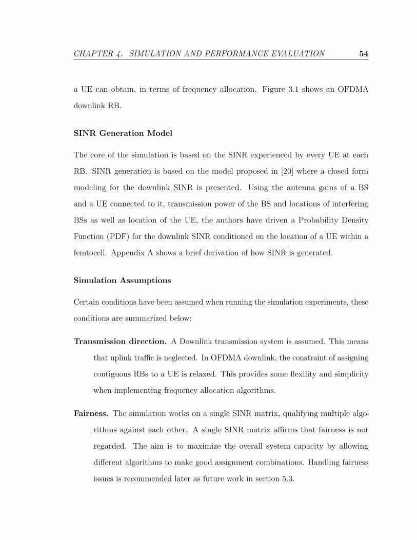
CHAPTER 4. SIMULATION AND PERFORMANCE EVALUATION 54
a UE can obtain, in terms of frequency allocation. Figure 3.1 shows an OFDMA
downlink RB.
SINR Generation Model
The core of the simulation is based on the SINR experienced by every UE at each
RB. SINR generation is based on the model proposed in [20] where a closed form
modeling for the downlink SINR is presented. Using the antenna gains of a BS
and a UE connected to it, transmission power of the BS and locations of interfering
BSs as well as location of the UE, the authors have driven a Probability Density
Function (PDF) for the downlink SINR conditioned on the location of a UE within a
femtocell. Appendix A shows a brief derivation of how SINR is generated.
Simulation Assumptions
Certain conditions have been assumed when running the simulation experiments, these
conditions are summarized below:
Transmission direction. A Downlink transmission system is assumed. This means
that uplink traffic is neglected. In OFDMA downlink, the constraint of assigning
contiguous RBs to a UE is relaxed. This provides some flexility and simplicity
when implementing frequency allocation algorithms.
Fairness. The simulation works on a single SINR matrix, qualifying multiple algo-
rithms against each other. A single SINR matrix affirms that fairness is not
regarded. The aim is to maximize the overall system capacity by allowing
different algorithms to make good assignment combinations. Handling fairness
issues is recommended later as future work in section 5.3.
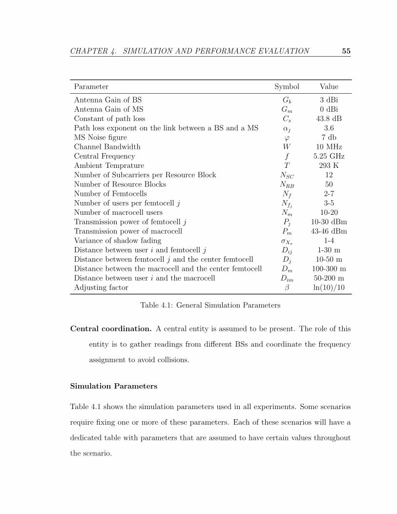
CHAPTER 4. SIMULATION AND PERFORMANCE EVALUATION 55
Parameter Symbol Value
Antenna Gain of BS Gb 3 dBiAntenna Gain of MS Gm 0 dBiConstant of path loss Cs 43.8 dBPath loss exponent on the link between a BS and a MS αj 3.6MS Noise figure ϕ 7 dbChannel Bandwidth W 10 MHzCentral Frequency f 5.25 GHzAmbient Temprature T 293 KNumber of Subcarriers per Resource Block NSC 12Number of Resource Blocks NRB 50Number of Femtocells Nf 2-7Number of users per femtocell j Nfj 3-5Number of macrocell users Nm 10-20Transmission power of femtocell j Pj 10-30 dBmTransmission power of macrocell Pm 43-46 dBmVariance of shadow fading σXs 1-4Distance between user i and femtocell j Dij 1-30 mDistance between femtocell j and the center femtocell Dj 10-50 mDistance between the macrocell and the center femtocell Dm 100-300 mDistance between user i and the macrocell Dim 50-200 mAdjusting factor β ln(10)/10
Table 4.1: General Simulation Parameters
Central coordination. A central entity is assumed to be present. The role of this
entity is to gather readings from different BSs and coordinate the frequency
assignment to avoid collisions.
Simulation Parameters
Table 4.1 shows the simulation parameters used in all experiments. Some scenarios
require fixing one or more of these parameters. Each of these scenarios will have a
dedicated table with parameters that are assumed to have certain values throughout
the scenario.
CHAPTER 4. SIMULATION AND PERFORMANCE EVALUATION 56
4.1.2 Candidate Algorithms
Chapter 2 provided a survey of recent works in the field of frequency allocation. The
surveyed works covered the techniques used in such field. A number of schemes have
been chosen to evaluate the performance of the proposed algorithm. These schemes
have been implemented to the best of our knowledge, to carry out the functions
intended originally by their authors in the referenced papers. We carefully chose the
closest techniques to our proposed scheme. We prioritized schemes that depended on
channel allocation over schemes that depended on power allocation. We were also
keen to choose schemes that are easy to implement in order not to miss any detail
that might compromise fairness in our simulation. The next section shows the results
of our choice.
4.1.3 Kim’s Algorithm
In [12], Kim et al. proposed a centralized, system capacity maximization algorithm.
The algorithm is two-fold: 1. Power allocation phase, and 2. Sub-channel allocation
phase. To match the objective function of this scheme with the proposed MCF, only
the sub-channel allocation part has been implemented. To maintain the simulation
assumptions in [20], transmission power of a BS is kept constant throughout a single
experiment. Two versions of this algorithm have been developed: a CSG version,
to match the simulation assumptions for the proposed MCF algorithm, and another
Open Subscriber Group (OSG) version to fully exploit the strength of Kim’s algorithm.
The difference between the two versions is that in a CSG environment, users are pre-
attached to their BSs, and hence, users are allocated RBs at the serving BS. Whereas
in the OSG version, a UE is allowed to switch to a better serving BS by means of
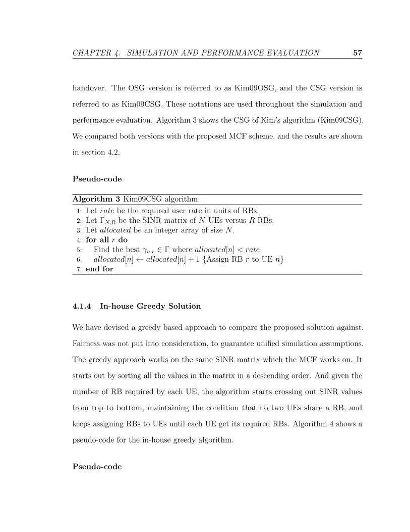
CHAPTER 4. SIMULATION AND PERFORMANCE EVALUATION 57
handover. The OSG version is referred to as Kim09OSG, and the CSG version is
referred to as Kim09CSG. These notations are used throughout the simulation and
performance evaluation. Algorithm 3 shows the CSG of Kim’s algorithm (Kim09CSG).
We compared both versions with the proposed MCF scheme, and the results are shown
in section 4.2.
Pseudo-code
Algorithm 3 Kim09CSG algorithm.
1: Let rate be the required user rate in units of RBs.2: Let ΓN,R be the SINR matrix of N UEs versus R RBs.3: Let allocated be an integer array of size N .4: for all r do5: Find the best γn,r ∈ Γ where allocated[n] < rate6: allocated[n]← allocated[n] + 1 {Assign RB r to UE n}7: end for
4.1.4 In-house Greedy Solution
We have devised a greedy based approach to compare the proposed solution against.
Fairness was not put into consideration, to guarantee unified simulation assumptions.
The greedy approach works on the same SINR matrix which the MCF works on. It
starts out by sorting all the values in the matrix in a descending order. And given the
number of RB required by each UE, the algorithm starts crossing out SINR values
from top to bottom, maintaining the condition that no two UEs share a RB, and
keeps assigning RBs to UEs until each UE get its required RBs. Algorithm 4 shows a
pseudo-code for the in-house greedy algorithm.
Pseudo-code
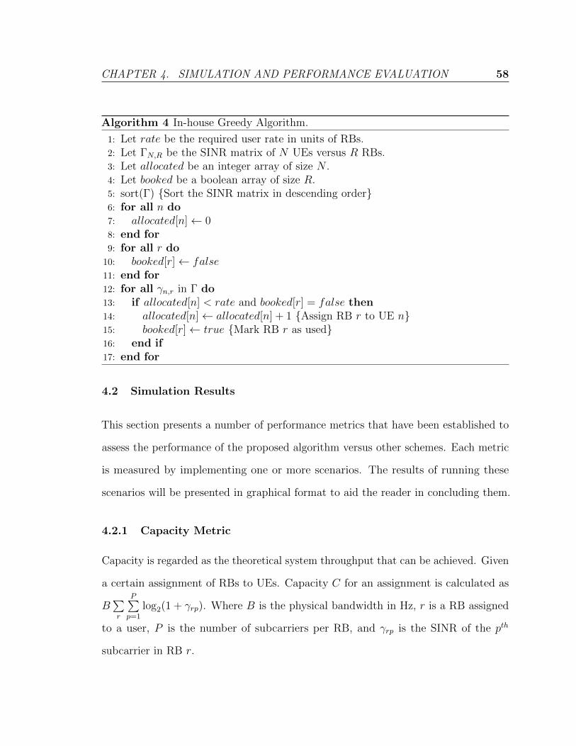
CHAPTER 4. SIMULATION AND PERFORMANCE EVALUATION 58
Algorithm 4 In-house Greedy Algorithm.
1: Let rate be the required user rate in units of RBs.2: Let ΓN,R be the SINR matrix of N UEs versus R RBs.3: Let allocated be an integer array of size N .4: Let booked be a boolean array of size R.5: sort(Γ) {Sort the SINR matrix in descending order}6: for all n do7: allocated[n]← 08: end for9: for all r do10: booked[r]← false11: end for12: for all γn,r in Γ do13: if allocated[n] < rate and booked[r] = false then14: allocated[n]← allocated[n] + 1 {Assign RB r to UE n}15: booked[r]← true {Mark RB r as used}16: end if17: end for
4.2 Simulation Results
This section presents a number of performance metrics that have been established to
assess the performance of the proposed algorithm versus other schemes. Each metric
is measured by implementing one or more scenarios. The results of running these
scenarios will be presented in graphical format to aid the reader in concluding them.
4.2.1 Capacity Metric
Capacity is regarded as the theoretical system throughput that can be achieved. Given
a certain assignment of RBs to UEs. Capacity C for an assignment is calculated as
B∑r
P∑p=1
log2(1 + γrp). Where B is the physical bandwidth in Hz, r is a RB assigned
to a user, P is the number of subcarriers per RB, and γrp is the SINR of the pth
subcarrier in RB r.
CHAPTER 4. SIMULATION AND PERFORMANCE EVALUATION 59
Experiment A1: Effect of changing number of users per femtocell
In this experiment, capacity is evaluated in response to changing the number of users
per femtocell. The experiment has been repeated 20 times per each value from the set
[1, 2, 3, 4, 5]. Table 4.2 identifies the experiment specific parameters that differ from
the general simulation parameters presented in table 4.1.
Parameter Symbol Value
Number of users per femtocell j Nfj [1, 2, 3, 4, 5]Number of Femtocells Nf 7Number of macrocell users Nm 15
Table 4.2: Experiment A1 specific parameters.
For each experiment run with a certain seed, all capacities attained from all schemes
are normalized relative to 100, i.e. the capacity value of the algorithm that scores best
is set to 100, and capacities from other algorithms are set to a percentage of the best
capacity, as in equation 4.1. Then, for each value of Nfj , all normalized capacities are
averaged as in equation 4.2
Normalized capacity at seed s =Capacity at seed s
Best capacity at seed s∗ 100 (4.1)
Normalized capacity at a certain value Nfj =
∑s
Normalized capacity at seed s
20
(4.2)
Figure 4.2 shows the simulation results of experiment A1. The proposed optimal
algorithm, MCF, outperforms all other schemes as expected. The in-house greedy
approach scores near optimal capacity, 0.5% to 1.0% less performance than optimal.
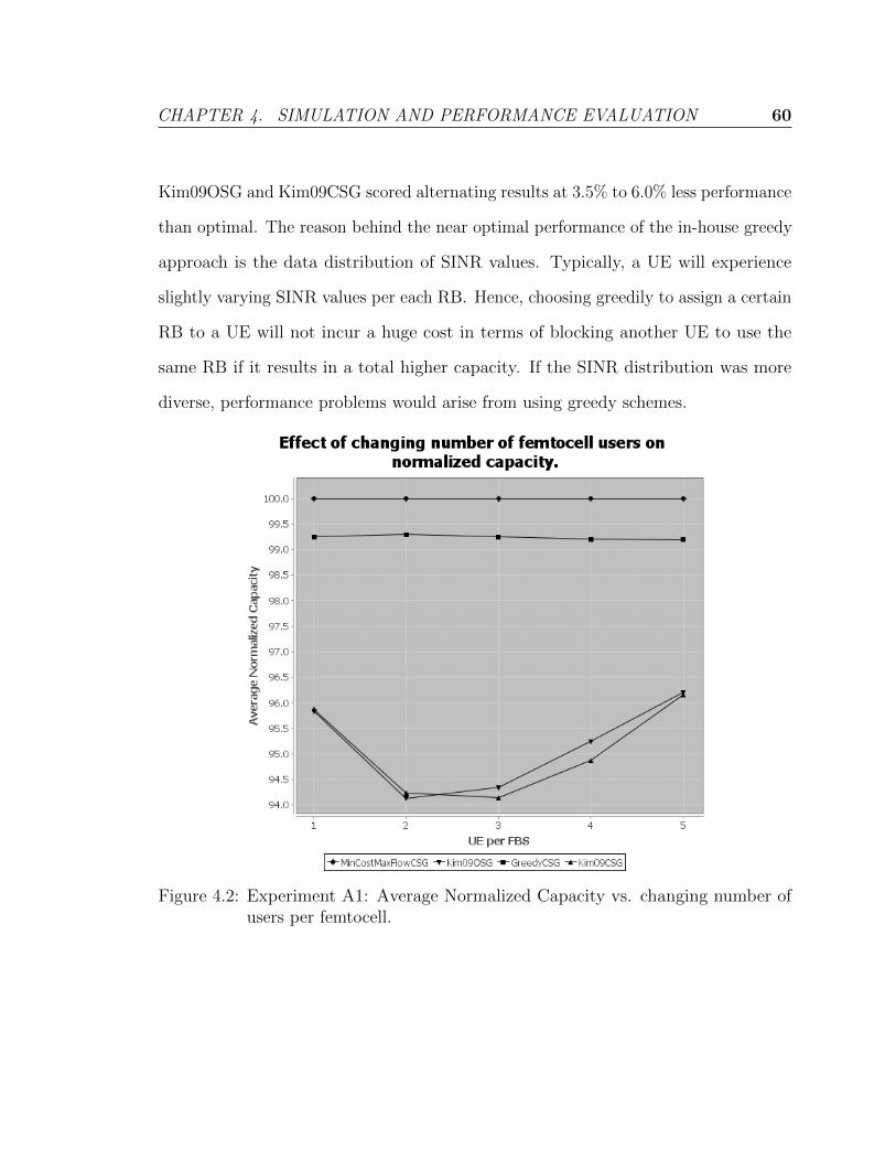
CHAPTER 4. SIMULATION AND PERFORMANCE EVALUATION 60
Kim09OSG and Kim09CSG scored alternating results at 3.5% to 6.0% less performance
than optimal. The reason behind the near optimal performance of the in-house greedy
approach is the data distribution of SINR values. Typically, a UE will experience
slightly varying SINR values per each RB. Hence, choosing greedily to assign a certain
RB to a UE will not incur a huge cost in terms of blocking another UE to use the
same RB if it results in a total higher capacity. If the SINR distribution was more
diverse, performance problems would arise from using greedy schemes.
Figure 4.2: Experiment A1: Average Normalized Capacity vs. changing number ofusers per femtocell.
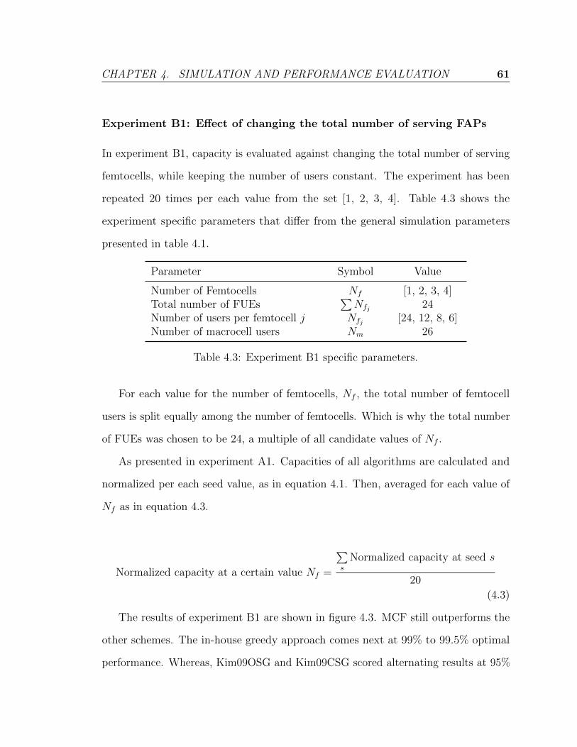
CHAPTER 4. SIMULATION AND PERFORMANCE EVALUATION 61
Experiment B1: Effect of changing the total number of serving FAPs
In experiment B1, capacity is evaluated against changing the total number of serving
femtocells, while keeping the number of users constant. The experiment has been
repeated 20 times per each value from the set [1, 2, 3, 4]. Table 4.3 shows the
experiment specific parameters that differ from the general simulation parameters
presented in table 4.1.
Parameter Symbol Value
Number of Femtocells Nf [1, 2, 3, 4]Total number of FUEs
∑Nfj 24
Number of users per femtocell j Nfj [24, 12, 8, 6]Number of macrocell users Nm 26
Table 4.3: Experiment B1 specific parameters.
For each value for the number of femtocells, Nf , the total number of femtocell
users is split equally among the number of femtocells. Which is why the total number
of FUEs was chosen to be 24, a multiple of all candidate values of Nf .
As presented in experiment A1. Capacities of all algorithms are calculated and
normalized per each seed value, as in equation 4.1. Then, averaged for each value of
Nf as in equation 4.3.
Normalized capacity at a certain value Nf =
∑s
Normalized capacity at seed s
20
(4.3)
The results of experiment B1 are shown in figure 4.3. MCF still outperforms the
other schemes. The in-house greedy approach comes next at 99% to 99.5% optimal
performance. Whereas, Kim09OSG and Kim09CSG scored alternating results at 95%
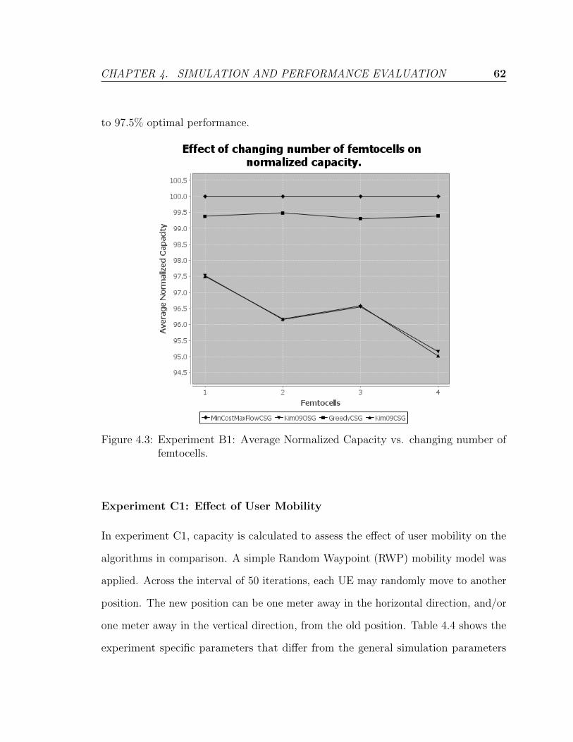
CHAPTER 4. SIMULATION AND PERFORMANCE EVALUATION 62
to 97.5% optimal performance.
Figure 4.3: Experiment B1: Average Normalized Capacity vs. changing number offemtocells.
Experiment C1: Effect of User Mobility
In experiment C1, capacity is calculated to assess the effect of user mobility on the
algorithms in comparison. A simple Random Waypoint (RWP) mobility model was
applied. Across the interval of 50 iterations, each UE may randomly move to another
position. The new position can be one meter away in the horizontal direction, and/or
one meter away in the vertical direction, from the old position. Table 4.4 shows the
experiment specific parameters that differ from the general simulation parameters
CHAPTER 4. SIMULATION AND PERFORMANCE EVALUATION 63
presented in table 4.1.
Parameter Symbol Value
Number of Femtocells Nf 4Number of users per femtocell j Nfj 4Total number of FUEs
∑Nfj 16
Number of macrocell users Nm 9
Table 4.4: Experiment C1 specific parameters.
As seen in table 4.4, the number of FUEs is 16, and the number of MUEs is 9, for
a total of 25 UEs. This results in two RBs per user.
The layout generation is done once at the beginning of this experiment. And the
positions of all UEs are updated at each iteration, by applying RWP mobility model,
as explained. The SINR matrix is calculated at each iteration as well, before the
algorithms run again for this iteration.
The results of experiment C1 are shown in figure 4.4. The proposed benchmark
MCF stays at the top, while the in-house greedy approach is just below it at 98.5% to
99.7% optimal performance. Kim09OSG and Kim09CSG fluctuate around 95.5% to
98% optimal performance.
In the experiments above, although a greedy scheme performed quite well versus
the optimal scheme, the other two approaches namely; Kim09OSG and Kim09CSG
did not reach such performance. The main drawback in Kim’s approach proposed
in [12] is that it deals with one RB at a time, trying to maximize the benefit (capacity
in this case) from using this RB. The problem is that a UE can be sufficiently served
from earlier RBs, leaving out better capacity RBs that might come later, and probably
wasting good RBs on other UEs. This flaw in Kim’s approach did not let it benefit
fully from being a greedy-based scheme.
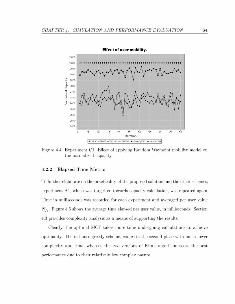
CHAPTER 4. SIMULATION AND PERFORMANCE EVALUATION 64
Figure 4.4: Experiment C1: Effect of applying Random Waypoint mobility model onthe normalized capacity.
4.2.2 Elapsed Time Metric
To further elaborate on the practicality of the proposed solution and the other schemes;
experiment A1, which was targetted towards capacity calculation, was repeated again.
Time in milliseconds was recorded for each experiment and averaged per user value
Nfj . Figure 4.5 shows the average time elapsed per user value, in milliseconds. Section
4.3 provides complexity analysis as a means of supporting the results.
Clearly, the optimal MCF takes more time undergoing calculations to achieve
optimality. The in-house greedy scheme, comes in the second place with much lower
complexity and time, whereas the two versions of Kim’s algorithm score the best
performance due to their relatively low complex nature.
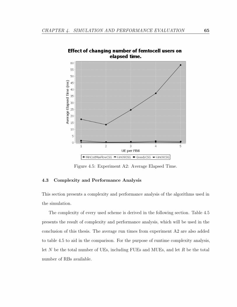
CHAPTER 4. SIMULATION AND PERFORMANCE EVALUATION 65
Figure 4.5: Experiment A2: Average Elapsed Time.
4.3 Complexity and Performance Analysis
This section presents a complexity and performance analysis of the algorithms used in
the simulation.
The complexity of every used scheme is derived in the following section. Table 4.5
presents the result of complexity and performance analysis, which will be used in the
conclusion of this thesis. The average run times from experiment A2 are also added
to table 4.5 to aid in the comparison. For the purpose of runtime complexity analysis,
let N be the total number of UEs, including FUEs and MUEs, and let R be the total
number of RBs available.
CHAPTER 4. SIMULATION AND PERFORMANCE EVALUATION 66
MCF Complexity
Algorithm 2 runs in iterations. It finds a shortest path in every iteration, assigning a
RB to a user, possibly reassigning another RB if needed. This makes the outer loop of
O(R) complexity. The call to Bellmanford shortest path depicted in Algorithm 1 has
a worst case complexity of O(V.E) where V is the size of vertices list and E is the
size of edges list. Since the generated graph is fully connected then V = R +N + 2
and E = R.N +R+N . Essentially, this comes from R RBs, each one is connected to
N UEs, in addition to N links to the artificial source and R links to the artificial sink.
Note that the dominant term is R.N .
Hence the total complexity of a MCF based on Bellmanford shortest path is
O(R.(R +N).(R.N)) = O(R2.N(R +N))
Kim’s Algorithm Complexity
The complexity analysis of algorithm 3 is pretty straight forward. It encompasses R
loops on all RBs, each has a maximum of N UEs to check. This brings the algorithm
to a complexity of O(N.R). Similarly, the OSG version of this algorithm, referred to
as Kim09OSG, is O(N.R.B), where B is the number of BSs.
Greedy In-house Scheme Complexity
Algorithm 4 starts by sorting out the SINR matrix, typically with complexityO(N.R) log(N.R).
The loop in lines 11-17 is of O(N.R). Since sorting is the dominating factor then the
algorithm complexity is of O(N.R) log(N.R)
Based on the results in table 4.5, recommendations will be provided in chapter 5,
which concludes this thesis.
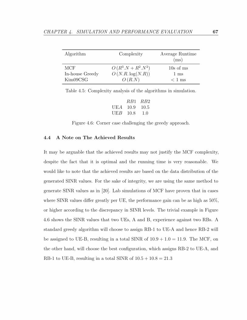
CHAPTER 4. SIMULATION AND PERFORMANCE EVALUATION 67
Algorithm Complexity Average Runtime(ms)
MCF O (R3.N +R2.N2) 10s of msIn-house Greedy O (N.R. log(N.R)) 1 msKim09CSG O (R.N) < 1 ms
Table 4.5: Complexity analysis of the algorithms in simulation.
RB1 RB2UEA 10.9 10.5UEB 10.8 1.0
Figure 4.6: Corner case challenging the greedy approach.
4.4 A Note on The Achieved Results
It may be arguable that the achieved results may not justify the MCF complexity,
despite the fact that it is optimal and the running time is very reasonable. We
would like to note that the achieved results are based on the data distribution of the
generated SINR values. For the sake of integrity, we are using the same method to
generate SINR values as in [20]. Lab simulations of MCF have proven that in cases
where SINR values differ greatly per UE, the performance gain can be as high as 50%,
or higher according to the discrepancy in SINR levels. The trivial example in Figure
4.6 shows the SINR values that two UEs, A and B, experience against two RBs. A
standard greedy algorithm will choose to assign RB-1 to UE-A and hence RB-2 will
be assigned to UE-B, resulting in a total SINR of 10.9 + 1.0 = 11.9. The MCF, on
the other hand, will choose the best configuration, which assigns RB-2 to UE-A, and
RB-1 to UE-B, resulting in a total SINR of 10.5 + 10.8 = 21.3
CHAPTER 5. SUMMARY AND CONCLUSION 68
Chapter 5
Summary and Conclusion
5.1 Summary
In this thesis we presented an introduction to femtocell networks and highlighted
the essence of establishing them. We also stressed that the application of newer
networks like LTE and LTE Advanced will require the existence of femtocells as a
step towards the logical evolution of small and personal BSs. We also presented the
interference problem in detail, and the importance of mitigation solutions in smooth
service provisioning.
We leveraged a representative set of proposals from the literature to combat inter-
ference. Several solutions exist that vary in nature (centralized versus distributed) and
at the level at which the solution is applied (femtocellular, femtocellular / macrocellu-
lar). Some solutions resort to transmission power management while others utilizes
frequency allocation. A comparison of some of these solutions was presented in chapter
2. Also, we proposed a novel and effective algorithm to address a definite void in the
literature to tackle outstanding problems in interference mitigation.
CHAPTER 5. SUMMARY AND CONCLUSION 69
We emphasize on the importance of interference mitigation to guarantee the
expected return from femtocell networks. The use of highly efficient algorithms has
been already proposed in the literature to complement traditional methods that rely
on pure optimizations to either the physical or the MAC layers. In [40] the need for
non-conventional network planning and optimization techniques has been motivated,
with assertions that distributed, self-optimized techniques are anticipated to produce
more reliable results than ordinary algorithms [15].
When multiple operators come into play [51], and with the introduction of LTE
networks and the notions of virtualization, ’global spectrum’ [52], and cognitive
radio [53], very high level of coordination is required to guarantee smooth operation
for all operators. A new class of cooperative techniques will emerge to cope with this
new network architecture [53, 54]. At the same time, self-optimization on the cell
level will be a critical feature to have because FBSs will no longer come from the
same provider, in addition to the large number of small cells introduced by femtocell
technology.
Heterogeneous Networks (HetNets) [17, 35,55], a recently introduced evolutionary
notion of networking, have been establishing the importance of cooperative multi-
operator environment. A HetNet comprises a number of mixed macrocells, remote
radio heads and low-power nodes such as picocell and femtocells. Main characteristics
of the HetNet architecture include: high degree of spatial reuse, enhanced indoor
coverage, and highly technically challenging environment [18]. Such environment
demonstrates a number of interference sources, for example: unplanned deployment,
power difference between nodes, and range expanded users.
CHAPTER 5. SUMMARY AND CONCLUSION 70
5.2 Conclusion
We presented the results of extensive simulations to assess the quality of the proposed
solution. Despite the outstanding results that the proposed solution demonstrated
against representatives from the literature, we confidently see that a carefully optimized
greedy algorithm will be sufficient - although not optimal - to use. Even with lots of
greedy based algorithms in the literature, the way the algorithm is devised and coded
makes a difference.
Chapter 4 shows the results of lab simulations that made us reach the conclusion
that although greedy is not optimal, but greedy is good. As long as channel models
follow certain non-random distributions, greedy performance will be the most accept-
able in terms of quality and complexity. Simulations showed that a carefully coded
greedy approach scored a performance of 99% optimal. Moreover, operators still have
the liberty to choose to achieve the remaining 1% at the extra small cost of complexity,
using algorithms like the proposed MCF.
5.3 Recommendations and Future Work
Certain constraints have been assumed when running the experimental simulation as
elaborated in section 4.1. These constraints were assumed to make the simulation more
focused and easier in implementation. However, in a real scenarios these restrictions
cease to exist. And the less constraints a simulation assumes, the more realistic it is.
This section provides some recommendations to overcome the simulation assumptions,
and can be considered as future work.
CHAPTER 5. SUMMARY AND CONCLUSION 71
5.3.1 Fairness Issues
As presented, MCF works on a two dimensional matrix of numbers, maximizing the
summation of values, under certain constraints. MCF in its core does not regard the
locations of the chosen values within the SINR mtarix. Hence, constraints are put to
limit the number of RBs per UE. However, as seen throughout this thesis, fairness
is totally ignored. We developed a recommendation based on Proportional Fairness
algorithms, to incorporate fairness in a MCF. The idea is to apply a fairness factor on
the SINR matrices at subsequent frames, to force a UE that has been served relatively
more than other UEs, to have its SINR levels reduced by some factor proportional.
This reduction factor is directly proportional to the amount of admission this UE has
gained.
5.3.2 Adding Support to Uplink
The proposed scheme was targetted to downlink only, because downlink frequency
assignment is easier to deal with due to the fact that assigned resources don’t have
to be contiguous. There is a number of tricks in MCF implementation that allows
adding specific constraints to the resulting assignment. For example, in a MCF graph,
controlling the flow values on the links from the artificial source to the UEs, controls
how many flow units can move through a certain UE node, or in other words control
how many RBs can be assigned. We have been investigating tweaks on the regular
MCF to add support of uplink transmission as well, however, at the time of writing
the thesis, these tweaks were not mature enough to report.
CHAPTER 5. SUMMARY AND CONCLUSION 72
5.3.3 Distributed Operation
The proposed scheme in this thesis assumes centralized operation. It assumes the
existence of a centralized entity that gathers SINR information from BSs and handle
frequency assignment properly to avoid collision. The amount of signalling needed to
interface with the centralized entity may be in some cases costly or intolerable. This
urges the development of a distributed version of the proposed scheme. In [19], the
authors propose a decentralized hashing algorithm to aid in identifying nodes in a
network in a distributed fashion. They provide a collision resolution mechanism as
well. This scheme can be incorporated with MCF to provide a distributed optimal
scheme.
BIBLIOGRAPHY 73
Bibliography
[1] International Telecommunications Union, “Key global telecom indicators for
the world telecommunication service sector.” http://www.itu.int/ITU-D/ict/
statistics/at_glance/KeyTelecom.html.
[2] S. Saunders, S. Carlaw, A. Giustina, R. R. Bhat, V. S. Rao, and R. Siegberg,
Femtocells: Opportunities and Challenges for Business and Technology. New
York, NY, USA: John Wiley and Sons, 2009.
[3] E. Dahlman, S. Parkvall, J. Skold, and P. Beming, 3G Evolution, Second Edition:
HSPA and LTE for Mobile Broadband. Academic Press, 2008.
[4] M.-S. Alouini and A. Goldsmith, “Area Spectral Efficiency of Cellular Mobile
Radio Systems,” vol. 2, pp. 652–656, May 1997.
[5] X. Chu, Y. Wu, L. Benmesbah, and W.-K. Ling, “Resource Allocation in Hy-
brid Macro/Femto Networks,” in Wireless Communications and Networking
Conference Workshops (WCNCW), 2010 IEEE, pp. 1–5, April 2010.
[6] Y. Bai, J. Zhou, and L. Chen, “Hybrid Spectrum Usage for Overlaying LTE Macro-
cell and Femtocell,” GLOBECOM 2009 - 2009 IEEE Global Telecommunications
Conference, pp. 1–6, November 2009.
BIBLIOGRAPHY 74
[7] M. Dohler, R. Heath, A. Lozano, C. Papadias, and R. Valenzuela, “Is the PHY
Layer Dead?,” Communications Magazine, IEEE, vol. 49, pp. 159–165, April
2011.
[8] J. Hoydis, M. Kobayashi, and M. Debbah, “Green Small-Cell Networks,” Vehicular
Technology Magazine, IEEE, vol. 6, pp. 37–43, March 2011.
[9] J. Zhang, G. D. L. Roche, and G. L. D. Roche, Femtocells: Technologies and
Deployment. John Wiley and Sons, Ltd., 2010.
[10] D. Lopez-Perez, A. Valcarce, and G. de La Roche, “OFDMA femtocells: A
roadmap on interference avoidance,” IEEE Communications Magazine, vol. 47,
pp. 41–48, September 2009.
[11] J. Cullen, “Radioframe presentation,” Femtocells Europe, June 2008.
[12] J. Kim and D.-H. Cho, “A Joint Power and Subchannel Allocation Scheme
Maximizing System Capacity in Dense Femtocell Downlink Systems,” in Per-
sonal, Indoor and Mobile Radio Communications, 2009 IEEE 20th International
Symposium on, pp. 1381–1385, September 2009.
[13] D. Knisely, T. Yoshizawa, and F. Favichia, “Standardization of Femtocells in
3GPP,” Communications Magazine, IEEE, vol. 47, pp. 68–75, September 2009.
[14] S. Carlaw, “IPR and The Potential Effect on Femtocell Markets,” Femtocells
Europe, June 2008.
[15] J.-H. Yun and K. Shin, “Adaptive Interference Management of OFDMA Fem-
tocells for Co-Channel Deployment,” Selected Areas in Communications, IEEE
Journal on, vol. 29, pp. 1225–1241, June 2011.
BIBLIOGRAPHY 75
[16] “Merrill Lynch. Wireless data growth: How far, how fast, and who wins?,” tech.
rep., Merrill Lynch, 2007.
[17] S.-M. Cheng, S.-Y. Lien, F.-S. Chu, and K.-C. Chen, “On Exploiting Cogni-
tive Radio to Mitigate Interference in Macro/Femto Heterogeneous Networks,”
Wireless Communications, IEEE, vol. 18, pp. 40–47, June 2011.
[18] D. Lopez-Perez, I. Guvenc, G. de la Roche, M. Kountouris, T. Quek, and J. Zhang,
“Enhanced Intercell Interference Coordination Challenges in Heterogeneous Net-
works,” Wireless Communications, IEEE, vol. 18, pp. 22–30, June 2011.
[19] K. Sundaresan and S. Rangarajan, “Efficient resource management in ofdma
femto cells,” in Proceedings of the tenth ACM international symposium on Mobile
ad hoc networking and computing, MobiHoc ’09, (New York, NY, USA), pp. 33–42,
ACM, 2009.
[20] K. W. Sung, H. Haas, and S. McLaughlin, “A Semianalytical PDF of Downlink
SINR for Femtocell Networks,” EURASIP Journal on Wireless Communications
and Networking, vol. 2010, pp. 1–10, 2010.
[21] H. Hristov, R. Feick, and W. Grote, “Improving indoor signal coverage by
use of through-wall passive repeaters,” in Antennas and Propagation Society
International Symposium, 2001. IEEE, vol. 2, pp. 158 –161 vol.2, 2001.
[22] V. Chandrasekhar, J. Andrews, and A. Gatherer, “Femtocell Networks: A Survey,”
Communications Magazine, IEEE, vol. 46, pp. 59–67, September 2008.
BIBLIOGRAPHY 76
[23] T. Nihtila, “Increasing Femto Cell Throughput with HSDPA Using Higher Order
Modulation,” in Networking and Communications Conference, 2008. INCC 2008.
IEEE International, pp. 49–53, May 2008.
[24] H. Claussen, “Performance of Macro- and Co-Channel Femtocells in a Hierarchical
Cell Structure,” in Personal, Indoor and Mobile Radio Communications, 2007.
PIMRC 2007. IEEE 18th International Symposium on, pp. 1–5, September 2007.
[25] G. Korinthios, E. Theodoropoulou, N. Marouda, I. Mesogiti, E. Nikolitsa, and
G. Lyberopoulos, “Early Experiences and Lessons Learned from Femtocells,”
Communications Magazine, IEEE, vol. 47, pp. 124–130, September 2009.
[26] K. Kim and C. Wang, “Enterprise voip in fixed mobile converged networks,”
in Multimedia Analysis, Processing and Communications (W. Lin, D. Tao,
J. Kacprzyk, Z. Li, E. Izquierdo, and H. Wang, eds.), vol. 346 of Studies in
Computational Intelligence, pp. 585–621, Springer Berlin / Heidelberg, 2011.
[27] M. Krichen, J. Cohen, and D. Barth, “File transfer application for sharing femto
access,” CoRR, vol. abs/1104.5150, 2011.
[28] H. Aki, M. C. Erturk, and H. Arslan, “Dynamic channel allocation schemes for
overlay cellular architectures,” in Proceedings of the 9th conference on Wireless
telecommunications symposium, WTS’10, (Piscataway, NJ, USA), pp. 67–71,
IEEE Press, 2010.
[29] T. Kahwa and N. Georganas, “A Hybrid Channel Assignment Scheme in Large-
Scale, Cellular-Structured Mobile Communication Systems,” Communications,
IEEE Transactions on, vol. 26, pp. 432–438, April 1978.
BIBLIOGRAPHY 77
[30] J. Sin and N. Georganas, “A Simulation Study of a Hybrid Channel Assign-
ment Scheme for Cellular Land-Mobile Radio Systems with Erlang-C Service,”
Communications, IEEE Transactions on, vol. 29, pp. 143–147, February 1981.
[31] W. Yue, “Analytical methods to calculate the performance of a cellular mo-
bile radio communication system with hybrid channel assignment,” Vehicular
Technology, IEEE Transactions on, vol. 40, pp. 453–460, May 1991.
[32] I. Guvenc, M.-R. Jeong, F. Watanabe, and H. Inamura, “A Hybrid Frequency
Assignment for Femtocells and Coverage Area Analysis for Co-channel Operation,”
Communications Letters, IEEE, vol. 12, pp. 880–882, December 2008.
[33] Y. Bai, J. Zhou, and L. Chen, “Hybrid Spectrum Sharing for Coexistence of
Macrocell and Femtocell,” in Communications Technology and Applications, 2009.
ICCTA ’09. IEEE International Conference on, pp. 162–166, October 2009.
[34] M. Bennis, L. Giupponi, E. Diaz, M. Lalam, M. Maqbool, E. Strinati,
A. De Domenico, and M. Latva-aho, “Interference Management in Self-organized
Femtocell Networks: The BeFEMTO Approach,” in Wireless Communication,
Vehicular Technology, Information Theory and Aerospace Electronic Systems
Technology (Wireless VITAE), 2011 2nd International Conference on, pp. 1–6,
March 2011.
[35] S.-P. Yeh, S. Talwar, G. Wu, N. Himayat, and K. Johnsson, “Capacity and
Coverage Enhancement in Heterogeneous Networks,” Wireless Communications,
IEEE, vol. 18, pp. 32–38, June 2011.
BIBLIOGRAPHY 78
[36] R.-T. Juang, P. Ting, H.-P. Lin, and D.-B. Lin, “Interference Management of Fem-
tocell in Macro-cellular Networks,” in Wireless Telecommunications Symposium
(WTS), 2010, pp. 1–4, April 2010.
[37] H.-C. Lee, D.-C. Oh, and Y.-H. Lee, “Mitigation of Inter-Femtocell Interference
with Adaptive Fractional Frequency Reuse,” in Communications (ICC), 2010
IEEE International Conference on, pp. 1–5, May 2010.
[38] T. Lee, H. Kim, J. Park, and J. Shin, “Dynamic fractional-frequency reuse for
femtocells,” in Proceedings of the 5th International Conference on Ubiquitous
Information Management and Communication, ICUIMC ’11, (New York, NY,
USA), pp. 80:1–80:6, ACM, 2011.
[39] F. Mazzenga, M. Petracca, R. Pomposini, F. Vatalaro, and R. Giuliano, “Algo-
rithms for Dynamic Frequency Selection for Femto-cells of Different Operators,”
in Personal Indoor and Mobile Radio Communications (PIMRC), 2010 IEEE
21st International Symposium on, pp. 1550–1555, September 2010.
[40] T. Akbudak and A. Czylwik, “Distributed Power Control and Scheduling for
Decentralized OFDMA Networks,” in Smart Antennas (WSA), 2010 International
ITG Workshop on, pp. 59–65, February 2010.
[41] Z. Bharucha, A. Saul, G. Auer, and H. Haas, “Dynamic resource partitioning
for downlink femto-to-macro-cell interference avoidance,” EURASIP Journal on
Wireless Communications and Networking, vol. 2010, pp. 2:1–2:12, January 2010.
[42] G. E. M. Zhioua, P. Godlewski, S. Hamouda, and S. Tabbane, “Quietest channel
selection for femtocells in ofdma networks,” in Proceedings of the 8th ACM
BIBLIOGRAPHY 79
international workshop on Mobility management and wireless access, MobiWac
’10, (New York, NY, USA), pp. 125–128, ACM, 2010.
[43] H. Claussen, L. Ho, and L. Samuel, “Self-optimization of Coverage for Femtocell
Deployments,” in Wireless Telecommunications Symposium, 2008. WTS 2008,
pp. 278–285, April 2008.
[44] N. Arulselvan, V. Ramachandran, S. Kalyanasundaram, and G. Han, “Distributed
Power Control Mechanisms for HSDPA Femtocells,” in VTC Spring 2009 - IEEE
69th Vehicular Technology Conference, pp. 1–5, April 2009.
[45] E. J. Hong, S. Y. Yun, and D.-H. Cho, “Decentralized Power Control Scheme
in Femtocell Networks: A Game Theoretic Approach,” in Personal, Indoor and
Mobile Radio Communications, 2009 IEEE 20th International Symposium on,
pp. 415–419, September 2009.
[46] C.-W. Chen, C.-Y. Wang, S.-L. Chao, and H.-Y. Wei, “Dance: a game-theoretical
femtocell channel exchange mechanism,” ACM SIGMOBILE Mobile Computing
and Communications Review, vol. 14, pp. 13–15, July 2010.
[47] V. Chandrasekhar, J. Andrews, T. Muharemovic, Z. Shen, and A. Gatherer,
“Power Control in Two-tier Femtocell Networks,” Wireless Communications, IEEE
Transactions on, vol. 8, pp. 4316–4328, August 2009.
[48] M. Sahin, I. Guvenc, M.-R. Jeong, and H. Arslan, “Handling CCI and ICI
in OFDMA Femtocell Networks Through Frequency Scheduling,” Consumer
Electronics, IEEE Transactions on, vol. 55, pp. 1936–1944, November 2009.
BIBLIOGRAPHY 80
[49] R. K. Ahuja, T. L. Magnanti, and J. B. Orlin, Network Flows: Theory, Algorithms,
and Applications. Englewood Cliffs, NJ: Prentice Hall, 1993.
[50] D. B. West, Introduction to Graph Theory (2nd Edition). Prentice Hall, Aug.
2000.
[51] F. Mazzenga, M. Petracca, R. Pomposini, and F. Vatalaro, “Improving qos of
femtocells in multi-operator environments,” in Trustworthy Internet (L. Salgarelli,
G. Bianchi, and N. Blefari-Melazzi, eds.), pp. 117–128, Springer Milan, 2011.
[52] E. K. Paik, S.-H. Lee, C. Lee, J. Han, C. Park, T. Kwon, and Y. Choi, “Service
Differentiation Using Mobile Femtocell Virtualization,” in Consumer Communi-
cations and Networking Conference (CCNC), 2010 7th IEEE, pp. 1–4, January
2010.
[53] R. Urgaonkar and M. J. Neely, “Opportunistic Cooperation in Cognitive Femtocell
Networks,” ArXiv e-prints, March 2011.
[54] K. Lee, O. Jo, and D.-H. Cho, “Cooperative Resource Allocation for Guaranteeing
Intercell Fairness in Femtocell Networks,” Communications Letters, IEEE, vol. 15,
pp. 214–216, February 2011.
[55] H. Li, J. Hajipour, A. Attar, and V. Leung, “Efficient HetNet Implementation
Using Broadband Wireless Access with Fiber-connected Massively Distributed
Antennas Architecture,” Wireless Communications, IEEE, vol. 18, pp. 72–78,
June 2011.
APPENDIX A. DERIVATION OF SINR PDF 81
Appendix A
Derivation of SINR PDF
This appendix provides a summary to the derivation of the downlink SINR matrix as
demonstrated in [20]. In short the authors calculate three PDFs to derive the PDF of
downlink SINR. The three PDFs are:
1. The PDF for the power received at a UE.
2. The PDF of the aggregated interference received at the same UE.
3. The PDF of the background noise value.
Given a BS at the center of a cell, call it Cell of Interest (CoI). The cell has a
radius R, and M UEs uniformly distributed within the radius of this cell. Without
loss of generality, the CoI can be assumed to be placed at the origin (0, 0). Using this,
an arbitrary UE m is located at (rm, rθ) where 0 ≤ rm ≤ R and 0 ≤ rθ ≤ 2π. Also,
the location of the jth interfering BS would be (rb(j), θb(j)).
To calculate the power received at UE m:
• P ts : transmission power of the BS at the CoI.
APPENDIX A. DERIVATION OF SINR PDF 82
• Gb: antenna gain of the BS at the CoI, Gm: the antenna gain of the UE.
• Cs: constant of path loss in the CoI.
• αs: path loss exponent of the CoI.
• XS: Gaussian random variable modeling the shadow fading, with zero mean
and σ2Xs
variance in db.
• β:ln 10
10.
The received signal power at UE m from the serving BS will be
P rs = P t
sGbGmCsr−αsm exp(βXs)
which can also be written as
P rs = exp
[ln(P t
sGbGmCs)− αs ln rm + (βXs)]
which follows a log-normal distribution [20], and thus the PDF conditional on the
location of the UE m is given by
fprs(z | rm, θm) =1
zσs√
2πexp
[−(ln z − µs)2
2σ2s
](A.1)
where µs = ln(P tsGbGmCs)− αs ln rm and σ2
s = β2σ2Xs
.
To calculate the interference at a UE m:
• P tj : transmission power from the jth BS.

APPENDIX A. DERIVATION OF SINR PDF 83
• Cj: path loss constant on the link between jth BS and UE m.
• αs: path loss exponent on the link between jth BS and UE m.
• Xj: Gaussian random variable modeling the shadow fading on the link between
jth BS and UE m, with zero mean and σ2Xj
variance in db.
• dmb(j): distance between jth BS and UEm=√
[r2m + rb(j)2 − 2rmrb(j) cos(θm − θb(j))].
The received interference power from the jth interfering BS will be
Irj = P tjGbGmCjdmb(j)
−αj exp(βXj)
which can also be modeled as a random variable in the form of Y = exp(X) as the
transmission power, and thus follows a log-normal distribution and its PDF is given
by:
fIrj (z | rm, θm) =1
zσj√
2πexp
[−(ln z − µj)2
2σ2j
](A.2)
where µj = ln(P tjGbGmCj)− αjdmb(j)) and σ2
j = β2σ2Xj
To calculate the background noise value Nbg:
• k: the Boltzmann constant.
• T : the ambient temperature in Kelvin.
• W : channel bandwidth.
• ϕ: Noise figure of the UE.
APPENDIX A. DERIVATION OF SINR PDF 84
Therefore Nbg = kTWϕ which can also be represented as a log-normal random variable
with a zero variance and mean µn = ln(kTWϕ) as follows
Nbg = exp(ln(kTWϕ) +Xn) (A.3)
given that Xn is a Gaussian random variable with zero mean and zero variance [20].
Using three log-normal random variables in equations (A.1, A.2 and A.3), the
downlink SINR of UE m is denoted by
γm =P rs
L∑i=1
Irj +Nbg
=P rs
Υ(A.4)
where Υ is the summation of all interference powers and background noise power,
and can also be approximated as a log-normal random variable [20].
The PDF of Υ conditioned on the location of UE m is
fΥ(z | rm, θm) =1
zσΥ
√2π
exp
[−(ln z − µΥ)2
2σ2Υ
](A.5)
where σ2Υ = ln
L+1∑j=1
exp(2µj + σ2
j
) (exp
(σ2j
)− 1)
[L+1∑j=1
exp(µj +
σ2j
2
)]2 + 1
,
µΥ = ln
[L+1∑j=1
exp(µj +
σ2j
2
)]− σ2
Υ
2
Equations A.1, A.5 and A.4 are used to generate the SINR experienced for all UEs,
by repeating the same steps for all UEs at all cells.