Interference Analysis And Mitigation Of Telemetry (tm) And

University of Texas at El PasoDigitalCommons@UTEP

Open Access Theses & Dissertations

2018-01-01

Interference Analysis And Mitigation Of Telemetry(tm) And 4g Long-Term Evolution (lte) Systems InAdjacent Spectrum BandsJuan Francisco GonzalezUniversity of Texas at El Paso, [email protected]

Follow this and additional works at: https://digitalcommons.utep.edu/open_etdPart of the Electrical and Electronics Commons

This is brought to you for free and open access by DigitalCommons@UTEP. It has been accepted for inclusion in Open Access Theses & Dissertationsby an authorized administrator of DigitalCommons@UTEP. For more information, please contact [email protected].

Recommended CitationGonzalez, Juan Francisco, "Interference Analysis And Mitigation Of Telemetry (tm) And 4g Long-Term Evolution (lte) Systems InAdjacent Spectrum Bands" (2018). Open Access Theses & Dissertations. 1441.https://digitalcommons.utep.edu/open_etd/1441

https://digitalcommons.utep.edu/?utm_source=digitalcommons.utep.edu%2Fopen_etd%2F1441&utm_medium=PDF&utm_campaign=PDFCoverPages

https://digitalcommons.utep.edu/open_etd?utm_source=digitalcommons.utep.edu%2Fopen_etd%2F1441&utm_medium=PDF&utm_campaign=PDFCoverPages

https://digitalcommons.utep.edu/open_etd?utm_source=digitalcommons.utep.edu%2Fopen_etd%2F1441&utm_medium=PDF&utm_campaign=PDFCoverPages

http://network.bepress.com/hgg/discipline/270?utm_source=digitalcommons.utep.edu%2Fopen_etd%2F1441&utm_medium=PDF&utm_campaign=PDFCoverPages

https://digitalcommons.utep.edu/open_etd/1441?utm_source=digitalcommons.utep.edu%2Fopen_etd%2F1441&utm_medium=PDF&utm_campaign=PDFCoverPages

mailto:[email protected]

INTERFERENCE ANALYSIS AND MITIGATION OF TELEMETRY (TM)

AND 4G LONG-TERM EVOLUTION (LTE) SYSTEMS

IN ADJACENT SPECTRUM BANDS

JUAN FRANCISCO GONZALEZ

Master’s Program in Electrical Engineering

APPROVED:

Virgilio Gonzalez, Ph.D., Chair

Bryan Usevitch, Ph.D.

Filiberto A. Macias, M.S.

Pabel Corral

Susumu “Duke” Yasuda

Charles Ambler, Ph.D.

Dean of the Graduate School

Copyright ©

by

Juan Francisco Gonzalez

2018

Dedication

to my loving family

my parents

Francisco Javier & María del Rocío

and my siblings

Javier Eliseo, Rocío, and Margarita

for their unconditional support and guidance

INTERFERENCE ANALYSIS AND MITIGATION OF TELEMETRY (TM)

AND 4G LONG-TERM EVOLUTION (LTE) SYSTEMS

IN ADJACENT SPECTRUM BANDS

by

JUAN FRANCISCO GONZALEZ, B.S.E.E.

THESIS

Presented to the Faculty of the Graduate School of

The University of Texas at El Paso

in Partial Fulfillment

of the Requirements

for the Degree of

MASTER OF SCIENCE

Department of Electrical and Computer Engineering

THE UNIVERSITY OF TEXAS AT EL PASO

May 2018

v

Acknowledgements

I would like to express my deepest gratitude to Dr. Virgilio Gonzalez of the Electrical and

Computer Engineering Department at The University of Texas at El Paso, for his consideration,

guidance, never-ending knowledge, and patience. "Keep It Simple and S." is a phrase that will be

engraved in my academic and professional practice; as for the last 'S', probably only Dr. Gonzalez,

Pablo, and I will recognize it. Dr. Gonzalez showed me the way to do things effectively and in a

simpler manner, to not overcrowd my thoughts and to focus on what the real issue is. He also

taught me to learn how to express my thoughts and to land whatever is in my head to a piece of

paper. I wish more students had the opportunity to experience his knowledge and determination.

I would also like to appreciate the organization and techniques that Dr. Pablo Rangel

employed during this project. I honestly do not know how he could keep track of everything and

do it effectively, it was impressive. I learned a lot from Dr. Rangel's practices and his determination

to execute a project, and I am very thankful that he always showed his support to me.

A thank you is also directed to Dr. Joel Quintana, for displaying his dedication and material

to Dr. Rangel and me. Also, for including us in discussions about current events, as this helped me

keep my mind rolling and to let me know that I should also take care of what is outside.

I also wish to thank the other members of my committee, of the Electrical and Computer

Engineering Department, both at The University of Texas at El Paso. Their suggestions, comments

and additional guidance were invaluable to the completion of this work.

Furthermore, I would like to thank The University of Texas at El Paso Electrical and

Computer Engineering Department professors and staff for all their hard work and dedication,

providing me the means to complete my degree and prepare for a career as an electrical engineer.

And finally, I must thank my friends and family for always showing support, being with

me, understanding the hardship of being in graduate school, and for participating in playful banter

to make ourselves laugh and distract me from just working from morning to midnight. I do not

vi

have the words to express all my feelings here, but I want them all to know that this would not

have been possible if it not for their collective support.

Being able to reach this point in my career has been a challenging experience, from working

several jobs and spending most of my time at school, I will always be thankful for all the people

who have guided me through. And I will especially be thankful for having the opportunity to share

all these wonderful years with Alejandra Escajeda Figueroa, I will like to give her my utmost

gratitude for being part of my life during these years and those to come.

Thank you all.

vii

NOTE: This thesis was submitted to my Supervising Committee in the Spring of 2018.

Abstract

Currently, the telecommunications, radio systems, and many other wireless services in the

United States are using the spectrum from the 6 kHz to the 300 GHz frequencies. Although it may

seem enough for said systems, as more users and devices are being introduced into the market, the

spectrum is limiting the faster introduction of these devices and/or systems. The radio frequency

spectrum is home to many transmissions, from amateur radio to cellphone applications, which all

share similar frequency bands. By sharing, the number of applications can be increased in a single

band, but their performance may be affected. Herein, experiments describing the relationship of

LTE and Telemetry systems are displayed, in order to classify the behavior of these systems under

close operation.

The Federal Communications Commission (FCC) oversees regulating interstate and

international communications by radio, television, wire, satellite and cable. It played an important

role in the FCC Auction 97, commonly known as Advanced Wireless Services-3 (AWS-3). The

White Sands Missile Range (WSMR) was the main user to be affected in this auction, since there

was a considerable loss in the military reserved spectrum. Provided herein are background

information, systems involved in the mitigation, overview of the spectrum usage, and data

collection from the spectrum involving AWS-3. An experiment on a testbed is described and

analyzed to simulate communication systems present in said bands, in order to observe the

viii

interaction between each other. This with the purpose of providing rules for a more efficient use

of the spectrum, and for suggesting mitigation techniques to the WSMR users.

The primary focus of this document is to explore what solutions there are to adjacent

interfering bands. This to be able to operate normally without any hindrance from external systems;

meaning that the wireless systems from WSMR are to not interfere with the 4G LTE Uplink and

Downlink bands, and vice-versa. Since fines exists for any type of interference done on other

channels, economical aspects that influence the behavior of the WSMR systems are also included.

Performance metrics will be gathered in the testbed, to understand what happens with interference,

and to determine the best practices for both systems to coexist harmoniously.

Also included is a brief introduction of the fifth-generation standard for wireless

communications (5G), by exploring and explaining the current trends to be able to implement this

standard into today's systems. It may be of interest to merge onto a new faster, more reliable, and

of higher data network; hence why it is included. The 5G network will build on to what the 4G

LTE network already has, the purpose is to enhance its capabilities and pave the way for the

Internet of Things (IoT).

ix

Table of Contents

Acknowledgements ..........................................................................................................................v

Abstract ......................................................................................................................................... vii

Table of Contents ........................................................................................................................... ix

List of Tables ................................................................................................................................ xii

List of Figures .............................................................................................................................. xiii

List of Illustrations ..................................................................................................................... xviii

Chapter 1: Introduction ....................................................................................................................1

Chapter 2: Literature Review ...........................................................................................................3

Chapter 3: Background Information ................................................................................................6

3.1 Radio Frequency Spectrum ...............................................................................................6

3.1.1 L, S, and C-bands ..................................................................................................7

3.2 Limitations of the Spectrum with respect to Shannon-Hartley .........................................9

3.3 Software Defined Radio ..................................................................................................10

3.4 Cellular Standards and Frequency Table ........................................................................11

3.5 Antenna Basics................................................................................................................12

Chapter 4: Methodology ................................................................................................................15

4.1 Database ..........................................................................................................................15

4.2 Frequency Bands of Interest ...........................................................................................16

4.3 System Experiment .........................................................................................................18

4.4 Composition and Expectation .........................................................................................19

4.5 Testbed Implementation..................................................................................................20

4.5.1.1 Numerical Parameters .............................................................................23

4.5.1.2 Visual Parameters ...................................................................................24

4.6 Testbed Adjustments .......................................................................................................27

4.7 Experiment Description ..................................................................................................29

Chapter 5: Results ..........................................................................................................................31

5.1 Baseline Parameters ........................................................................................................31

5.1.1 LTE Downlink (eNB station to UE device) ........................................................31

x

5.1.2 LTE Uplink (UE device to eNB station).............................................................35

5.1.3 Telemetry Baseline Characteristics .....................................................................35

5.2 Telemetry Interference on LTE Systems ........................................................................41

5.2.1 Lower L-band......................................................................................................42

Equal power levels output by the TM and LTE systems ....................................42

TM power increased above the LTE power level ...............................................48

5.2.2 Upper L-band ......................................................................................................51



5.2.3 Lower S-band ......................................................................................................58



5.2.4 Upper S-band ......................................................................................................65



5.2.4 Lower C-band .....................................................................................................70



5.2.5 Middle C-band ....................................................................................................76



5.3 LTE Interference on Telemetry Systems ........................................................................80

5.3.1 Lower L-band......................................................................................................81

5.3.2 Upper L-band ......................................................................................................85

5.3.3 Lower S-band ......................................................................................................88

5.3.3 Upper S-band ......................................................................................................91

5.3.4 Lower C-band .....................................................................................................94

5.3.4 Middle C-band ....................................................................................................97

xi

Chapter 6: Conclusions ..................................................................................................................99

References ....................................................................................................................................102

Glossary .......................................................................................................................................104

Vita 106

xii

List of Tables

Table 3.1: Digital Cellular Operating Bands ................................................................................ 12

Table 4.1: Telemetry bands of interest. ........................................................................................ 16

Table 4.2: FDD LTE bands & frequencies. .................................................................................. 17

xiii

List of Figures

Figure 3.1: Close-up look of the 72 - 124 MHz range, as established by the NTIA. ..................... 7

Figure 3.2: AWS-3 bands involved. The upper-L band of interest is highlighted by the yellow

box1. ................................................................................................................................................ 7

Figure 3.3: L-band spectrum users and frequencies. ...................................................................... 8

Figure 3.4: S-band spectrum users and frequencies........................................................................ 9

Figure 3.5: C-band spectrum users and frequencies. ...................................................................... 9

Figure 3.6: Visual representation of the composition of the types of radios employed nowadays.

....................................................................................................................................................... 11

Figure 3.7: Radio link and purpose of the antennas...................................................................... 12

Figure 3.8: Expected loss in polarization mismatch. .................................................................... 13

Figure 3.9: Radiation pattern of a dipole antenna. ........................................................................ 14

Figure 3.10: Additional radiation parameters. .............................................................................. 14

Figure 4.2: Basic experimental layout for the communication systems employed. ..................... 18

Figure 4.3: Final testbed implementation with the Telemetry source, LTE interference source,

noise source, and the digital filter. Two spectrum analyzers were used to observe the behavior

before and after filtering the signals. ............................................................................................ 21

Figure 4.4: Constellation Diagram for a BPSK signal (rotated 90° for illustration purposes). This

image was generated using the testbed. ........................................................................................ 25

Figure 4.5: Two-length eye diagram for a BPSK signal. Image generated with the testbed. ....... 25

Figure 4.6: An ASK eye diagram. Generated only for illustration purposes. ............................... 26

Figure 4.7: SNR vs BER plot for a simulated OFDM signal for illustration purposes only. ....... 26

Figure 4.8: Spectrum of an LTE downlink signal without amplification. .................................... 28

Figure 4.9: Spectrum of an LTE downlink signal with an amplifier. ........................................... 28

Figure 5.1: LTE DL OFDM Carrier with no interference. ........................................................... 32

Figure 5.2: The received signal from the UE to the eNB station. ................................................. 33

Figure 5.3: Throughput and BLER for a clean UL signal. ........................................................... 33

Figure 5.4: Plot of the BLER over time. ....................................................................................... 34

Figure 5.5: Constellation Diagram of a QPSK UL channel.......................................................... 34

Figure 5.6: Transmitted LTE UL channel signal. ......................................................................... 35

Figure 5.7: A clean BPSK transmitted signal with a 150 kHz bandwidth. ................................... 36

xiv

Figure 5.8: BPSK constellation rotated 90 degrees. ..................................................................... 37

Figure 5.9: Eye diagram of a clean BPSK signal.......................................................................... 37

Figure 5.10: The received BPSK signal. ....................................................................................... 38

Figure 5.11: Received BPSK constellation diagram..................................................................... 39

Figure 5.12: The Rx 2-length eye diagram for a BPSK signal. .................................................... 39

Figure 5.13: Tx constellation diagram of an OQPSK signal. ....................................................... 40

Figure 5.14: Rx constellation diagram for an OQPSK signal. ...................................................... 41

Figure 5.15: OQPSK TM signal and LTE DL signal in adjacent bands. The center frequency is

1.445 GHz. .................................................................................................................................... 43

Figure 5.16: BLER for the LTE system. ....................................................................................... 43

Figure 5.17: Constellation, data rate over time, and throughput for the LTE system. ................. 44

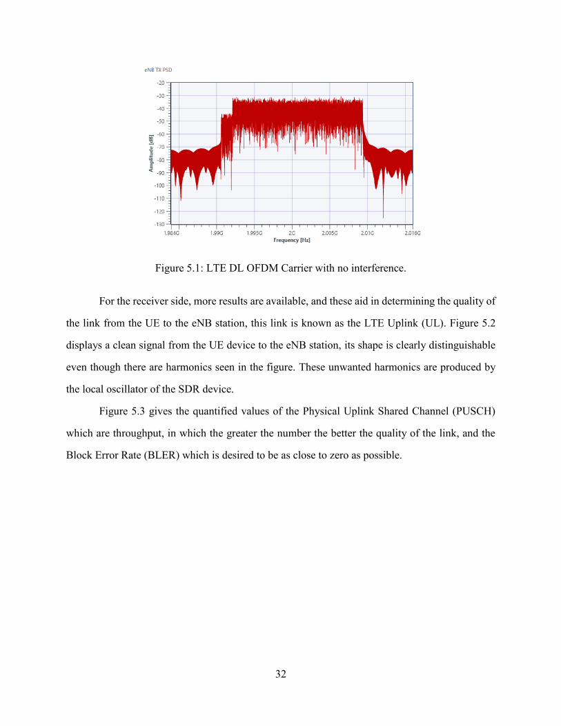
Figure 5.19: BLER graph for the current scenario. ...................................................................... 45

Figure 5.20: More measurements for the LTE system. ................................................................ 46

Figure 5.21: Both TM and LTE signals overlapping. ................................................................... 47

Figure 5.22: BLER for the LTE system with the TM overlapped signal. .................................... 47

Figure 5.23: Constellation graph and data rate drop as well as throughput for the LTE system. . 48

Figure 5.24: Spectrum graph of the two signals, with the TM system having more power than the

LTE signal. .................................................................................................................................... 49

Figure 5.25: BLER of the scenario. .............................................................................................. 49

Figure 5.26: More parameters to qualify and quantify the scenario. ............................................ 50

Figure 5.27: Spectrum graph and BLER graph for the described scenario. ................................. 51

Figure 5.28: Additional parameters for qualification and quantification of the scenario. ............ 51

Figure 5.29: Spectrum and BLER graph for the current scenario. The spectrum analyzer was

centered at 1.8 GHz....................................................................................................................... 52

Figure 5.30: Additional qualification and quantification parameters for the scenario. ................ 53

Figure 5.31: Spectrum and BLER graphs for the current configuration. No interference detected.

....................................................................................................................................................... 54

Figure 5.32: Additional parameters for the LTE system. No detrimental interference observed. 54

Figure 5.33: Spectrum and BLER graph for the current scenario. BLER starts to vary. ............. 55

Figure 5.34: More performance metrics, the throughput does not see much of a change. ........... 55

Figure 5.35: Spectrum and BLER graphs for the current experiment. ......................................... 56

xv

Figure 5.36: Constellation and data rate parameters for the current experiment. ......................... 56

Figure 5.37: Spectrum and BLER graphs for the current experiment. ......................................... 57

Figure 5.38: Constellation diagram, data rate graph, and throughput metrics. ............................. 57

Figure 5.39: Spectrum and the LTE BLER graph of the current experiment. .............................. 59

Figure 5.40: Additional metrics for measuring the LTE performance. ........................................ 59

Figure 5.41: Spectrum and LTE BLER graph for the experiment. ............................................... 60

Figure 5.42: Additional metrics to aid in the quantification and qualification of the link. .......... 60

Figure 5.43: The spectrum graph shows both signals overlapping, and the LTE BLER shows the

result of this................................................................................................................................... 61

Figure 5.44: Additional parameters that show that the LTE link is still in decent operation. ...... 62

Figure 5.45: Spectrum graph and the LTE BLER graph for the current scenario. ....................... 63

Figure 5.46: The parameters obtained here reinforce the figure above. ....................................... 63

Figure 5.47: Spectrum graph for the TM and LTE signals and BLER graph for the LTE system.

....................................................................................................................................................... 64

Figure 5.48: Constellation diagram and data rate graph for the LTE system. .............................. 64

Figure 5.49: Spectrum graph of the signals, and BLER of the LTE system. ................................ 66

Figure 5.50: Constellation and data rate graphs. ........................................................................... 66

Figure 5.51: Both TM and LTE signals overlapping in the spectrum graph while the LTE BLER

remains at zero. ............................................................................................................................. 67

Figure 5.52: Jittery constellation graph and constant data rate. .................................................... 67

Figure 5.53: Spectrum graph and LTE BLER graphs for the current experiment. ....................... 68

Figure 5.54: Additional parameters that prove the LTE system works normally. ........................ 69

Figure 5.55: Spectrum graph of the two signals and LTE BLER graph. ...................................... 70

Figure 5.56: These metrics show that the performance of the LTE system was degraded due to

the TM signal. ............................................................................................................................... 70

Figure 5.57: Spectrum graph and BLER for the LTE system with no TM interference. ............. 72

Figure 5.58: Constellation and data rate. ...................................................................................... 72

Figure 5.59: Spectrum graph of the TM and LTE systems at the lower C-band, as well as the

BLER for the LTE system. ........................................................................................................... 73

Figure 5.60: The constellation diagram is jittery, although the throughput remained very similar

to the C-band baseline value. ........................................................................................................ 73

xvi

Figure 5.61: Spectrum graph of the two signals 15 MHz apart, and the BLER of the LTE system

that indicates the interference was significant. ............................................................................. 74

Figure 5.62: Constellation diagram and data rate for the LTE system. ........................................ 74

Figure 5.63: The spectrum graph shows that the TM signal overpowers the LTE signal by a small

factor, and the BLER graph shows that the link has some errors but remains operational. ......... 75

Figure 5.64: Constellation diagram and the data rate graph that shows the link is still operational.

....................................................................................................................................................... 75

Figure 5.65: Spectrum graph of the semi-overlapping signals and the BLER at a high value. .... 76

Figure 5.66: Completely scattered and jittery constellation with a throughput of zero. ............... 76

Figure 5.67: Spectrum graph of the signals and BLER graph of the TM system. ........................ 77

Figure 5.68: Clear constellation diagram and decent data rate for the LTE system. .................... 78

Figure 5.69: Spectrum graph of the signals in the middle C-band and the affected BLER. ......... 78

Figure 5.70: Clear constellation but low data rate and throughput. .............................................. 79

Figure 5.71: Spectrum graph and a high BLER for the LTE system. ........................................... 80

Figure 5.72: Constellation diagram with a very low throughput graph. ....................................... 80

Figure 5.73: Spectrum of the TM and LTE signals 20 MHz apart. The FSER graph of the TM

system shows that the interference was not detrimental. .............................................................. 83

Figure 5.74: Additional parameters to qualify the OQPSK TM link. The constellation diagram,

spectrum received, and eye diagram. ............................................................................................ 83

Figure 5.75: Spectrum graph and FSER of the TM system. ......................................................... 84

Figure 5.76: Constellation diagram, spectrum graph with increased noise floor, and eye diagram.

....................................................................................................................................................... 84

Figure 5.77: Overlapped signals and FSER graph that shows that at certain instances where the

FSER was 1. .................................................................................................................................. 85

Figure 5.78: Jittery constellation, spectrum graph, and eye diagram. .......................................... 85

Figure 5.79: Spectrum graph and FSER. ...................................................................................... 87

Figure 5.80: Parameters seen by the TM receiver. Constellation diagram, spectrum graph, and

eye diagram. .................................................................................................................................. 87

Figure 5.81: Spectrum analyzer graph shows how the signals are overlapping, yet a small peak

can be seen that represents the TM signal. The FSER graph shows that there were some errors in

the system...................................................................................................................................... 88

xvii

Figure 5.82: Jittery constellation diagram, spectrum graph with a higher noise floor, and an

unrecognizable eye........................................................................................................................ 88

Figure 5.83: Spectrum graph of the signals and FSER plot of the TM system. ........................... 90

Figure 5.84: Constellation diagram, spectrum graph as seen by the TM Rx, and eye diagram. .. 90

Figure 5.85: Spectrum graph with the TM signal barely noticeable, and FSER plot of the system.

....................................................................................................................................................... 91

Figure 5.86: Qualitative graphs for the TM system with LTE interference. ................................ 91

Figure 5.87: TM and LTE signals together. Spectrum graph and FSER. ..................................... 92

Figure 5.88: Constellation diagram, TM Rx spectrum graph, and eye diagram. .......................... 93

Figure 5.89: Spectrum graph and FSER for the TM system......................................................... 93

Figure 5.90: Jittery constellation, spectrum as seen by the TM Rx, and eye diagram. ................ 94

Figure 5.91: Spectrum graph of the TM system at a lower C-band frequency. ............................ 95

Figure 5.92: Additional visual parameters for the TM system at a high frequency. .................... 95

Figure 5.93: Spectrum graph of the TM and LTE signals, and the FSER for the TM system. .... 96

Figure 5.94: Jittery constellation diagram, with noisy spectrum seen by the TM Rx, and eye

diagram. ........................................................................................................................................ 96

Figure 5.96: Spectrum average graph of the LTE and TM signals, as well as the FSER for the

TM system. ................................................................................................................................... 98

Figure 5.97: Spectrum graph of the signals 25 MHz apart, with an improved FSER than Figure

5.96................................................................................................................................................ 98

xviii

List of Illustrations

Illustration 4.1: Two views of the testbed. The four SDR devices in charge of transmitting and

receiving are present, as well as their connections. On the left side, the splitters and combiners

are shown. ..................................................................................................................................... 22

Illustration 4.2: SDR device utilized in filtering.4.5.1 Testbed Parameters ................................. 22

Illustration 4.3: Spectrum analyzing equipment used for detecting the signals being sent by the

SDRs. The top one is the pre-filtering stage and the bottom one is the post-filtering stage. ........ 23

Illustration 4.4: Amplifier used before the filter input. The red pin represents the 5 V DC supply,

and the black pin represents ground.............................................................................................. 29

1

Chapter 1: Introduction

The radio frequency spectrum is being readjusted to fit the consumer need for mobile data

and applications, and these readjustments bring problems to the existing users of the spectrum.

With this, many spectrum management techniques are required to ensure the normal operation of

the communication systems participating in adjacent spectrum bands. One of the solutions to

understand and classify the readjustment of communication systems in the spectrum, is to create a

flexible testbed that will be able to emulate said systems. This to predict the behavior of

interference and to create rules of interaction between systems to prevent interference. Described

herein, are techniques to mitigate interference between LTE and Telemetry communication

systems for purposes of spectrum allocation and interference mitigation.

The Federal Communications Commission (FCC) made available 65 megahertz (MHz) of

reserved spectrum for commercial use, as described in Auction 97 Advanced Wireless Services

(AWS-3) [1]. In the 1755 – 1780 MHz band, 25 MHz of military spectrum will be removed for

commercial use, and the current use of the 1755 – 1780 MHz band will be allocated into the 1780

– 1850 MHz band. Telemetry systems, radars, aviation, radio services, and cellular networks are

some of the users of the spectrum. The challenge is to place the previous mentioned systems into

the same band without causing noticeable interference or decreasing performance. A possible

solution is to coordinate joint usage of the radio spectrum for communications and other radio

frequency system applications. By identifying and classifying spectrum users, an optimal

assignation of spectral resources is to be proposed. AWS-3 loss mitigation is of utmost importance,

as it will be the concept that defines the set of rules or procedures that will have to be followed to

ensure optimal conditions to prevent major losses in the communication systems.

With the classification of spectrum users, a high-level network architecture will be

recommended, as well as tools to create a backbone similar to telecommunications service

providers to allow leverage of existing technologies. The evolved architecture must consider the

support and coexistence for some type of legacy technologies already deployed for

2

communications, and telemetry. The testbed will test and evaluate devices, tools, options and

solutions to the communications and radio operations for the military. Finally, a database of all

known signals that interact within the WSMR radio spectrum will be implemented. Since the

existing users are already in service and cannot be totally replaced overnight, Software Defined

Radio (SDR) equipment will be utilized to simulate said assets in service to ensure that the

proposed solution will function properly. The results from the experimentation will help determine

if an equipment replacement process is necessary, or if an adjustment with the current equipment

will suffice. These simulations and testing will generate data that will be placed in the database.

All the simulation results will be gathered to reach accurate conclusions that aid in the decision of

selecting which users can coexist in the spectrum band.

By using a SDR, spectrum users can be identified and classified depending on their

required power, spectrum usage, modulation scheme, Signal-to-Noise Ratio (SNR),

communication technology (Wi-Fi, 4G LTE, Bluetooth, etc.), behavior between signals,

bandwidth, and data rate. Recollection will be then stored into a database that will allow the

manipulation of data to prove concepts and to determine solutions.

Filtering solutions will also be considered to eliminate the interference that some systems

may pose on another, e.g., a Long-Term Evolution (LTE) system on a telemetry system. A situation

where an existing system will be considered as an interfering user to an LTE system will be tested,

as well as an LTE system interfering an existing system. Since legacy systems are present, this

testing method will be the focus to prevent numerous modifications to the existing systems.

In summary, to counteract the loss of spectrum to WSMR due to auctions made by the FCC

to allow more use of the spectrum for telecommunication companies, a testbed was developed to

study the interaction between systems with the hopes of creating rules of interaction and

interference mitigation techniques.

3

Chapter 2: Literature Review

Thesis Statement: Spectrum management and spectrum decongestant practices have

proven to be effective in the allocation of spectrum to users depending on their hierarchy or

assigned use by the NTIA. Currently, a portion of the military reserved spectrum was reassigned

to commercial users (AT\&T, Verizon, Sprint, T-Mobile, etc.) in a process known as AWS-3. The

spectrum management techniques described herein will help generate the rules that are needed

for optimal performance in communication systems sharing adjacent bands.

This thesis has as a basis the journal article titled “White Sands Missile Range (WSMR)

Radio Spectrum Enterprise Testbed: A Spectrum Allocation Solution” published in the ITEA

Journal on June 2017 by the authors Juan. F Gonzalez (self), Pablo Rangel, and Virgilio Gonzalez,

Ph.D., and it encompasses the basic testbed described herein. It also explains the process of how

the results are going to be obtained through the testbed, and what each of the components oversee.

It also mentions the database for the documents that are required to understand this material and

to determine the correct rules of interaction between systems to reduce interference [2].

The testbed has a heavy inspiration on the work that Kip Temple provides in his paper

titled “An Initial Look at Adjacent Band Interference Between Aeronautical Mobile Telemetry and

Long-Term Evolution Wireless Service” [3] in which he describes the AWS-3 auction and how

wireless services and technologies will be affected in this auction. He describes the technologies

involved and how the carriers interact when they are near, which is a study that is also being

conducted herein. The testbed and the experiments draw heavily from this paper by Temple.

In Cotton et al.'s [4] conference paper, the U.S. department of commerce employed a

Spectrum Monitoring Pilot Program to recollect data present in the federated spectrum, these data

would then be developed into a Measured Spectrum Occupancy Database (MSOD). This program

is useful to the thesis in that it gives an example of how to acquire spectrum data for analysis, since

the focus of the thesis is in spectrum management techniques; and with the sensing system

described herein, the data generated by the test bed can be obtained in a similar fashion.

4

The National Advanced Spectrum and Communications Test Network [5] created a draft

report where they provide robust test processes and validate measurement data. Described herein

is an established test methodology and measure of the out of band emissions (OOBE) from LTE

user equipment (UE) and evolved NodeB base stations (eNB) activities in the U.S. AWS-3

frequency band into the adjacent L frequency band.

For the LTE Performance Analysis, in Yang et al.s' [6] an extensive analysis of the LTE's

characteristics, such as: modulation and coding schemes, MIMO, transmit diversity, spatial

multiplexing, channel estimation, block error rate, and spectral efficiency, between many others.

With these characteristics, the systems employed in the thesis can be classified and understood

extensively.

As far as for telemetry operation, in the Quasonix Advanced Modulation Techniques for

Telemetry course [7], there are explanations of how to create telemetry systems, how to obtain the

performance metrics, modulation and demodulation, Forward Error Correction (FEC) and

performance comparisons. With this basis, the system described in the thesis can be effectively

created using these characteristics, and it will be certain that test bed will act similar to currently

existing telemetry systems.

In Souryal et al.'s [6] and in Temple's [3] journal article and report, respectively, the

architecture for the test beds are displayed. All sharing a similar fashion of a transmitter and

receiver system, interference source (system) and noise. While also acquiring data through

monitoring the signal power, error rates, and observing the behavior of the systems. This

architecture will serve to detect, implement, sample, and to analyze the systems and the spectrum.

In the Range Commanders Council (RCC) Telemetry Group's document titled Telemetry

Standards [8], as the title suggests, all the telemetry parameters, definitions, standards, and

frequency allocations were obtained from said document. It is of paramount importance to this

thesis, since most of the information contained in the thesis is heavily referenced in this document.

It was prepared by the RCC to "foster the compatibility of telemetry transmitting, receiving, and

signal processing equipment".

5

Spectrum Management Overview by T. Tjelta and R. Struzak [9] explains the current needs

for spectrum utilization in mobile services and personal wireless communication systems. It also

gives a quick introduction on how the electromagnetic -waves are related to the radio spectrum.

Although the paper focuses more on how federal regulation authorities should control the spectrum

use, it is worth mentioning that the technology applications will impact greatly how these

regulations should be generated. The testbed could assist in the legislation of the regulations

mentioned in order to aid the authorities in simulating the communication systems in the

discussion.

In the Dynamic Spectrum Management: Complexity and Duality journal article by Z. Q.

Luo and Z. Zhang [10], the authors consider a scenario where a "multiuser communication system"

has a standard approach to reduce interference, by diving the spectrum into "tones" or more

adequately, bands. The use solely a mathematical approach in scenarios such as multiple users and

multiple bands, or few users and many bands, in order to maximize the sharing of the spectrum. It

does not employ the use of a testbed, instead, it uses a computational approach to determine the

correct sizing of the bands, and the number of users that can be present in order to use the spectrum

efficiently. It is worth mentioning that this practice could be used to justify the correct bandwidth

of the signals employed in the testbed.

The literature mentioned before aids the author in determining the best practices for

creating a testbed that will emulate the scenarios described in the literature. Also, the literature

aids in explaining the telemetry concepts as well as the LTE characteristics. Some of the results

from the experiment can be compared to the results obtained in some of the literature reviewed,

with this, a close comparison can be done to determine the validity of the results presented herein.

6

Chapter 3: Background Information

This chapter was solely created to aid the reader in refreshing certain topics that are needed

to understand the material presented herein.

3.1 RADIO FREQUENCY SPECTRUM

The Radio Frequency Spectrum encompasses the frequencies from 3 kHz to 300 GHz, and

it is regulated in totality by the FCC. The National Telecommunications and Information

Administration (NTIA) is the entity who assigns specific frequency ranges -known as frequency

bands- to users who employ radio services. These users include telecommunications companies

(Verizon, AT&T, T-Mobile, Sprint, etc.), federal, military, amateur, research, radio and television

broadcasting, location services, and amateur users.

These users have to adjust to only using the frequencies in which they are allowed to

operate, failure to do so will result in fines imposed by the FCC Enforcement Bureau (FCCEB)

[11]. Some limitations exist, and users of their respective bands must employ their own

communications techniques to be able to operate in those frequencies at their desired conditions.

Figure 3.1 is a portion of the United States Frequency Allocations, it displays what users there are,

and at what band they operate [5].

Those are some of the users that exists in the spectrum. And those users have to restrain to

only using the frequencies they were allocated in. Otherwise, the FCCEB will have to take an

enforcement action.

As mentioned before, the AWS-3 affected primarily the WSMR personnel, as their 1755 –

1780 MHz band had to be auctioned to the telecommunication companies for LTE Uplink; and

their systems were reassigned to the 1780-1850 MHz band, also known as upper L-band. The

adjacent users of the upper L-band are shown in Figure 3.2, where adjacent users to the band of

interest are shown. Notice that the use of this band is for AMT [3] and for Space Operation (Earth-

to-Space).

7

Figure 3.1: Close-up look of the 72 - 124 MHz range, as established by the NTIA1.

Figure 3.2: AWS-3 bands involved. The upper-L band of interest is highlighted by the yellow

box1.

The experiments performed will be mainly focused the L, S, and C-bands, since these are

the bands that are affected by the AWS auctions.

3.1.1 L, S, and C-bands

Below are the spectrum snippets for the main bands of interest, this nomenclature follows

the IEEE frequency band designations [12]. These are highly linked to military and commercial

1 [5]

8

use. Figure 3.3 displays the current users of the L-band (from 1 - 2 GHz) and the frequencies of

interested are highlighted in the red boxes. This band was auctioned during the AWS-3.

Figure 3.3: L-band spectrum users and frequencies1.

The S-band (from 2 - 4 GHz) is the following band that will be included in the AWS-4,

and a portion of it is depicted in Figure 3.4. The frequencies of interest are highlighted in the red

boxes. Experiments were mainly conducted in the L and S-bands.

Finally, the C-band (4 - 8 GHz) will be the band of interest as well. It is mainly for future

reference, and since it is not as crowded as the previously mentioned bands, if the equipment allows

it, it can be utilized. A portion of it and its applications can be seen in Figure 3.5.

9

Figure 3.4: S-band spectrum users and frequencies1.

Figure 3.5: C-band spectrum users and frequencies1.

3.2 LIMITATIONS OF THE SPECTRUM WITH RESPECT TO SHANNON-HARTLEY

These spectrum allocations done by the NTIA play an important role in the channel

capacities of the users. The Shannon-Hartley equation 𝐶 = 𝐵 ∗ log2(1 + 𝑆𝑁𝑅) approximates the

maximum rate at which information can be transmitted, where 𝐶 is the channel capacity (bits per

second), 𝐵 is the bandwidth (Hz), and the 𝑆𝑁𝑅 is the signal-to-noise (SNR) ratio. The SNR is

obtained by dividing the average signal power 𝑆 and the average power of the noise 𝑁. This SNR

10

ratio (𝑆/𝑁) is important to look at, since the higher it is, the easier it is to decode the information

at the receiver, and if the resulting ratio falls below a value of one, then usually other spectrum

techniques are employed to be able to transmit data.

In part, the NTIA limits the amount of data that can be transmitted by a user. Although

there are techniques to reduce the amount of bandwidth needed, such as to increase the SNR, they

are not enough to outweigh the benefits of using a large amount of bandwidth. The users usually

do not use their whole spectrum band to transmit, they use "chunks" of spectrum. These chunks

can be assumed to be channels inside a spectrum band.

3.3 SOFTWARE DEFINED RADIO

Software Defined Radio (SDR) is "Radio in which some or all of the physical layer

functions are software defined" [13], which basically means that instead of leaving the hardware

to do the processing, up-conversion, sampling, modulation, etc., the software is now in charge of

performing these actions. Figure 3.6 is an example of the difference between the Traditional Radio,

Software Defined Radio, and Cognitive Radio. When comparing the traditional to the software

defined radio, the main difference is the amount of processing done by the hardware and the

software. It is easily seen that the SDR technique is migrating to mostly using software, as its name

suggests.

Cognitive Radio (CR) employs the same methods as SDR, it functions as an extension of

modern SDRs. It is an "aware radio" that has sensors and is aware of the environment [14]. By

employing machine learning, this CR can be taught to adapt to scenarios present in the spectrum.

For example, if a communications system is failing, the CR can determine to either increase the

transmission power, change the type of modulation, or readjust to an unused portion of the

spectrum (as long as it remains inside its established band).

11

Figure 3.6: Visual representation of the composition of the types of radios employed nowadays2.

3.4 CELLULAR STANDARDS AND FREQUENCY TABLE

Table 3.1 displays the frequencies used by the cellular bands, and the duplex mode that is

implemented in said bands of the Evolved Universal Terrestrial Radio Access (E-UTRA) [15].

Only the bands of interest are being considered. Uplink (UL) and Downlink (DL) frequencies are

usually separated, as they are not mixed, nor do they transmit the same amount of data. The UL

data rate is relatively smaller than the DL. In UL, only information from the User Equipment (UE)

is being sent to the LTE antenna (eNodeB or eNB). On the contrary, the DL portion of LTE, is

classified as the information sent from the eNB to the UE, and is greater in comparison to the data

rate of the UL.

These bands will be referenced throughout the document. It is important to familiarize with

the fact that most of these bands are adjacent to the telemetry bands that will be discussed later.

The distinction between the telemetry and the 4G-LTE bands will be done with greater clarity in

the subsequent chapters.

2 [20]

12

Table 3.1: Digital Cellular Operating Bands3

E-UTRA Operating Band

Uplink (UL) operating band

eNB receive

UE transmit

in MHz

Downlink (DL) operating band

eNB transmit

UE receive

in MHz

Duplex

Mode

𝑓𝑈𝐿 𝑙𝑜𝑤 − 𝑓𝑈𝐿 ℎ𝑖𝑔ℎ 𝑓𝐷𝐿 𝑙𝑜𝑤 − 𝑓𝐷𝐿 ℎ𝑖𝑔ℎ

1 1920 – 1980 2110 – 2170 FDD

2 1850 – 1910 1930 – 1990 FDD

4 1710 – 1755 2110 – 2155 FDD

7 2500 – 2570 2620 – 2690 FDD

22 3410 – 3490 3510 – 3590 FDD

23 2000 – 2020 2180 – 2200 FDD

25 1850 – 1915 1930 – 1995 FDD

30 2305 – 2315 2350 – 2360 FDD

33 1900 – 1920 1900 – 1920 TDD

40 2300 – 2400 2300 – 2400 TDD

42 3400 – 3600 3400 – 3600 TDD

43 3600 – 3800 3600 – 3800 TDD

3.5 ANTENNA BASICS

This section was mainly extracted from Rhode & Schwarz "Antenna Basics" [16].

In order to test a system wirelessly, antennas are strictly needed. The basic purpose of the

antenna in a communication system is shown in Figure 3.7: Radio link and purpose of the

antennas., where one needs the transmitting and receiver systems, as well as their respective

antennas, and a path of propagation which is usually air.

Figure 3.7: Radio link and purpose of the antennas4.

3 [21] 4 [16]

13

Also, it is worth mentioning that the antennas contain polarization that is determined by

the direction of an electric field. There are three types of polarization:

• Linear polarization

• Circular polarization

• Elliptical polarization

Polarization employs an important role in the synchronization of the signals. If the

polarization of the receiving antenna does not equal the polarization of the transmitting antenna,

or the incoming wave, a polarization mismatch will occur. In Figure 3.8, the losses due to mismatch

are pictured; where 'V' stands for vertical polarization, 'H' for horizontal polarization, 'LHC' for

left-hand circular polarization, and 'RHC' for right-hand circular polarization. This aids in the

understanding of losses in wireless communications systems, and/or mitigation of interference

between communication systems.

Figure 3.8: Expected loss in polarization mismatch4.

It is worth mentioning that the majority of antennas used in the testbed are dipoles. For

which their radiation patterns are shown in Figure 3.9, which makes it seem as a "donut" shaped

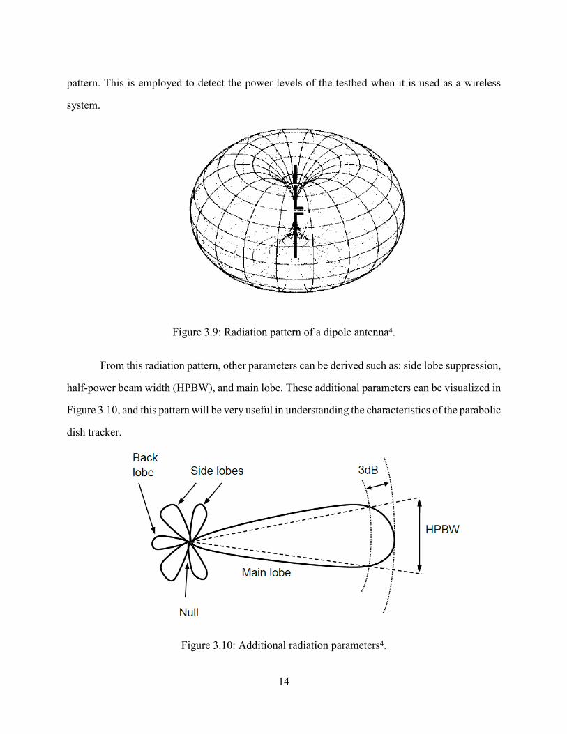
14

pattern. This is employed to detect the power levels of the testbed when it is used as a wireless

system.

Figure 3.9: Radiation pattern of a dipole antenna4.

From this radiation pattern, other parameters can be derived such as: side lobe suppression,

half-power beam width (HPBW), and main lobe. These additional parameters can be visualized in

Figure 3.10, and this pattern will be very useful in understanding the characteristics of the parabolic

dish tracker.

Figure 3.10: Additional radiation parameters4.

15

Chapter 4: Methodology

A comprehensive ontology was generated to explore the theoretical concepts of Radio

Frequency (RF) such as: fundamentals, bands, technology, applications, and uses, for the purpose

of defining the current situation of the spectrum and to provide theoretical solutions that will then

be tested on the experiments.

Several experiment scenarios will be designed to test the systems that will interact with

each other; and to observe the behavior between each other, and how to mitigate any interference.

The recorded data will aid in making better decisions regarding recommendations for the existing

systems.

This chapter is heavily inspired by the work presented in [2], as this document serves as a

continuation.

4.1 DATABASE

The ontology database is currently in a spreadsheet format. It will be translated into a

database language that will allow the thorough search of the content, and the display of the

references that were extracted.

The database contains the selected references of technical knowledge on signals and

systems, electromagnetic fields and waves, radio physics, data communications, antenna theory,

Software Defined Radio (SDR), Cognitive Radio (CR), spectrum analysis basics, telemetry,

frequency band nomenclature, cellular communication, wireless connectivity, Internet of Things

(IoT), and applications, and is the basis for classifying the users in the spectrum.

The criteria for classifying users in the spectrum will be based on the material of the

database. Figure 4. shows the procedure that will be used to generate the information in the

database, and what it will be used for.

16

Figure 4.1: Approach for the database creation and for its application.

4.2 FREQUENCY BANDS OF INTEREST

This section contains information on what frequencies were studied on the testbed. These

frequency bands were focused on since they are described in the IRIG-106 Telemetry Standards

document [8]. Also, the LTE frequency bands close to those of the telemetry standards were taken

into consideration.

The frequency bands that are of interest for telemetry are listed in Table 4.1. These

frequencies were used in the testbed since they are the ones established in the telemetry standards

document mentioned before. These frequencies should be taken into consideration in order to

simulate a more accurate telemetry system.

Table 4.1: Telemetry bands of interest.

Band Frequency Range (MHz) Application

L Lower 1435 – 1525 Mobile and Telemetry

Upper 1710 – 1990 Telemetry: 1780 – 1850 MHz

S Lower 2200 – 2290 Telemetry

Upper 2360 – 2395 Telemetry

C Lower 4400 – 4940 Telemetry

Mid 5090 – 5150 Telemetry

17

The frequency bands that are of interest for 4G-LTE simulation are shown in Table 4.2

[17]. These frequencies were also set in the testbed in order to simulate a more realistic

environment.

Table 4.2: FDD LTE bands & frequencies.

LTE Band Number UPLINK (UL) in MHz DOWNLINK (DL) in MHz

1 1920 – 1980 2110 – 2170

2 1850 – 1910 1930 – 1990

3 1710 – 1785 1805 – 1880

4 1710 – 1755 2110 – 2155

7 2500 – 2570 2620 – 2690

10 1710 – 1770 2110 – 2170

15 1900 – 1920 2600 – 2620

16 2010 – 2025 2585 – 2600

22 3410 – 3500 3510 – 3600

23 2000 – 2020 2180 – 2200

25 1850 – 1915 1930 – 1995

30 2305 – 2315 2350 – 2360

The main concern is for the telemetry system to function under interference from the LTE

source, and vice-versa. A coexistence of systems is paramount to this research.

18

4.3 SYSTEM EXPERIMENT

The top-level layout of the experiment that will be used to recollect data is depicted in

Figure 4.2 [2]. Each of the blocks are necessary to ensure a basic communications system with

added interference. A simulation of a telemetry and LTE systems is desired. The telemetry system

will be the main user and LTE will act as the interference for the main experiment, in order to

observe the behavior of these two systems in conjunction. Another test will be performed to

compare LTE as the main user and the telemetry system as a source of interference.

Figure 4.2: Basic experimental layout for the communication systems employed5.

The blocks in Figure 4.2 represent a hardware component that does a specific task. The

blocks Tx and Rx are part of the same communication system (LTE or Telemetry), while the M#

blocks are mitigation devices. The Interference Source and Noise blocks are in charge of

hampering the performance of the main communication system.

The general structure for the experiment is comprised of a transmitter (Tx), which will

begin as a telemetry system for the initial tests, and then it will swap the behavior to act as an LTE

system. An interference source will also be considered, this being first an LTE system whenever

our Tx is a telemetry system and vice-versa. Noise will be added to the system to emulate an actual

real-world situation; additive white Gaussian noise (AWGN) is considered. These previously

mentioned systems will each output a signal that will be added together in a mixer (represented by

5 [2]

19

the cross within the circle), to be acquired by the receiver (Rx). The system also contains mitigation

blocks (M1, M2, and M3), that will explore possible solutions to ensure that the data from Tx will

be received as accurate as possible in the Rx block. The operational values of the data signals such

as frequency, power (dBW), modulation scheme (QAM, PSK, BPSK, APSK, etc.), and bandwidth,

will be automated for the experimental data acquisition, while some will remain static in order to

find the natural variance of the system. Each of these operational values can be represented as a

series of combinations that will yield different results. For this experiment, the values employed

will have to be similar to those of current systems in order to obtain unbiased or more accurate

results. Frequency will remain static in the selected bands, while power from both Tx, interference

source, and noise will be variant. Modulation schemes will be similar to those used in today’s

standards, and some will be experimented with to see if there are modulation schemes that perform

better than others.

The experiment will explore different type of mitigations for the blocks such as filters,

amplifiers, attenuators, and/or forward error correction (FEC) codes. At the end, the target is for

the Frame Synchronization Error Rate (FSER) to be at zero. It is important to note that the

experiments might use an available anechoic chamber to simulate our system without causing any

disturbances to the FCC. Meaning that the system will be completely isolated from the exterior,

and the only sources of noise and interference will be created in the experiment.

The parameters for these tests will be adjusted accordingly to the data that will be collected

from the spectrum sensors located at the WSMR.

4.4 COMPOSITION AND EXPECTATION

All the tests will be performed without using classified information and the data transmitted

will be randomly generated. The SDR devices will emulate hardware and data link parameters of

existing WSMR using consumer civil standards (any technology proprietary to WSMR that is not

for public release is not included). Both the LTE and the telemetry systems will have their own

20

enclosure to have an unbiased system test. The Tx, Rx, interference source, and noise components

will be SDR devices, and the blocks M1, M2, and M3 will be either physical devices or SDR

functional blocks. These entities will perform the techniques that will mitigate interference.

What is expected from this experiment is to determine the best practices to mitigate the

interference between systems, if any. Simulations to determine said practices will be comprised of

software and hardware components.

4.5 TESTBED IMPLEMENTATION

With the utilization of SDRs and components such as coaxial cables, splitters and

combiners, the final testbed was developed. One SDR was used to generate a Telemetry transceiver

that included several PSK modulation schemes. Two other SDRs were used as the LTE system

(interference source), one device was used as the User Equipment (UE), e.g. a cellphone; the other

device acted as the eNodeB (eNB) station, or antenna. And the last SDR device was simply used

as the AWGN source.

All the outputs (TX) sources from the SDRs are combined into a final SDR device that is

in charge of filtering out the LTE signal, to leave the Telemetry signal clean. It is implied that a

certain amount of noise will not be filtered, which will affect the system. This noise and the amount

of unfiltered LTE (if any) will determine the performance and quality of the Telemetry system.

Lastly, after the filtering stage, the output will be split into four links which will go into

the Telemetry, LTE, and Spectrum Analyzer devices. This final configuration can be easily seen

in Figure 4.3, where each of the devices is labeled accordingly for easier readability. The devices

can be easily deactivated through software, or simply disconnected, in order to observe the

different behavior of the communications systems. The LTE can be deactivated, or the noise,

which would in theory, yield a clean Telemetry signal, and vice-versa.

21

Many types of filters were observed and tested, although the best performing filter

appeared to be a Chebyshev bandpass filter. The cutoff frequencies were set to the low and high

frequencies of the telemetry bands, this to attenuate the LTE signal as much as possible.

With the flexibility of the testbed, all the systems could be generated with ease and without

any violations to the FCC since it has the capability to work in a closed loop system. A wireless

test was conducted, but in a 2.4 GHz band that is considered the ISM band (industrial, scientific,

and medical radio) and with a power below 100 mW, again, to avoid any violations to the FCC

rulings.

Figure 4.3: Final testbed implementation with the Telemetry source, LTE interference source,

noise source, and the digital filter. Two spectrum analyzers were used to observe

the behavior before and after filtering the signals.

The physical layout of the testbed is presented in Illustration 4.1, it encompasses the SDRs

and the splitters in a closed controlled configuration. The filtering device, which is also a SDR is

represented in Illustration 4.2. These are presented with the purpose of aiding the reader into

understanding the layout clearly. There are two spectrum analyzers used for detecting the signals

in the radio frequency spectrum, the equipment used is presented in Illustration 4.3. Different

22

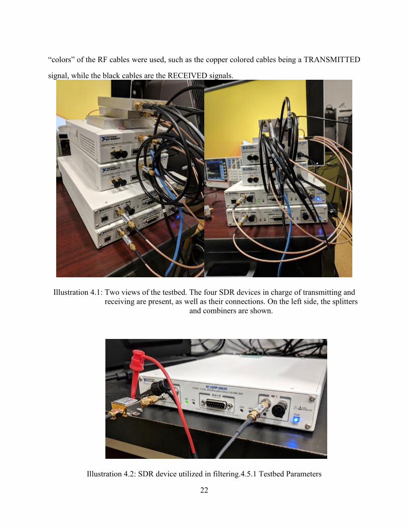
“colors” of the RF cables were used, such as the copper colored cables being a TRANSMITTED

signal, while the black cables are the RECEIVED signals.

Illustration 4.1: Two views of the testbed. The four SDR devices in charge of transmitting and

receiving are present, as well as their connections. On the left side, the splitters

and combiners are shown.

Illustration 4.2: SDR device utilized in filtering.4.5.1 Testbed Parameters

23

Illustration 4.3: Spectrum analyzing equipment used for detecting the signals being sent by the

SDRs. The top one is the pre-filtering stage and the bottom one is the post-

filtering stage.

For the testbed, two types of parameters were obtained: numerical and visual. Each of these

parameters are found in the testbed's software implementation. The numerical parameters' main

purpose is to quantify the performance of the testbed, while the visual parameters are used to

qualify performance.

4.5.1.1 Numerical Parameters

To quantify the performance of the system, numerical parameters must be obtained. These

parameters were obtained in the L, S, and the lower C-band, mainly in the border regions between

the telemetry and the LTE frequency bands.

It is important to notice the performance in different frequency bands to see how they differ

depending on what frequency band they are in (if any).

The numerical parameters are:

24

• Antenna Gain

o G/t

• Bandwidth (BW) of the Transmitted Signal

• BER or BLER (in LTE systems)

o Typically required to be ≤ 10−6

• Center Frequency (fc)

• Data Rate

• FSER

o Most likely required to be zero

• I/Q Rate

• Modulation Scheme

• Noise Floor

o Noise Factor/Figure (if applicable)

▪ Can be calculated by the input SNR vs output SNR when passing

through a device. Or by output noise vs thermal noise.

• Rx Power

o Rx Sensitivity Level (detection threshold)

• SNR

• Tx Power

All these quantifying parameters are to be obtained in the frequencies described, while

focusing mainly on the telemetry frequencies and their border bands.

4.5.1.2 Visual Parameters

To qualify the performance of the system, visual parameters must also be obtained along

with the numerical parameters. In every of the tests performed for the numerical parameters, the

visual parameters have to be observed —mainly through a spectrum analyzer or a Vector Network

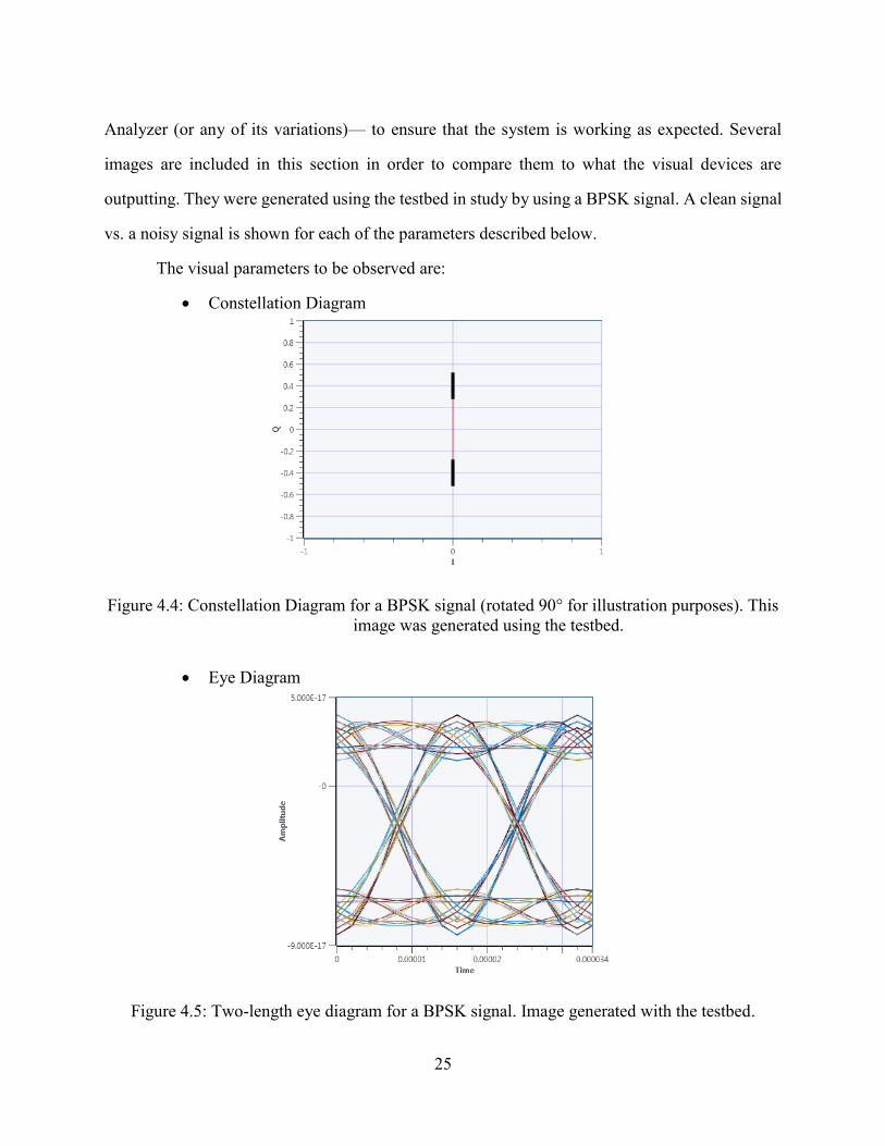
25

Analyzer (or any of its variations)— to ensure that the system is working as expected. Several

images are included in this section in order to compare them to what the visual devices are

outputting. They were generated using the testbed in study by using a BPSK signal. A clean signal

vs. a noisy signal is shown for each of the parameters described below.

The visual parameters to be observed are:

• Constellation Diagram

Figure 4.4: Constellation Diagram for a BPSK signal (rotated 90° for illustration purposes). This

image was generated using the testbed.

• Eye Diagram

Figure 4.5: Two-length eye diagram for a BPSK signal. Image generated with the testbed.

26

Figure 4.6: An ASK eye diagram. Generated only for illustration purposes.

• SNR vs BER/BLER

Figure 4.7: SNR vs BER plot for a simulated OFDM signal for illustration purposes only.

• Spectrum Graphs

• Waterfall Graph

27

These results are useful to help classify the testbed and the experiments in a numerical and visual

way. Compliance values are usually set by the consumer, although the main values of concern are

the Tx power, FSER, data rate, and SNR. Again, these values will help classify the performance

of the experiment scenario.

4.6 TESTBED ADJUSTMENTS

Since the signals are constantly being split and combined, an amplifying stage was

necessary the tests. Each of the splitters divided the power equally among its ports, and since the

splitting stage consists of a 1:2 splitter to the input of the filter and the spectrum analyzer, the

power loss was considerable, even if the transmission was at maximum power (20 dBm). This

meant that the power seen in the LTE framework UE receiver was averaging at -95 dBm as seen

in Figure 4.8: Spectrum of an LTE downlink signal without amplification.Figure 4.8, whereas with

the amplifying stage, a power of -55 dBm was obtained, which yielded greater results as seen in

Figure 4.9. This was the reasoning behind using an amplifying stage to adjust the testbed so that it

would encompass both scenarios. There will be two amplification stages (if necessary), the one

will occur at the filter input, and the other will occur before the 1:4 splitter.

28

Figure 4.8: Spectrum of an LTE downlink signal without amplification.

Figure 4.9: Spectrum of an LTE downlink signal with an amplifier.

Illustration 4.4 shows the configuration for the amplifier into the receiver of the filter. A 5

V DC voltage supply was used to power the amplifier. The amplifier had an average gain of 20

dB, the average was calculated by using the value of the gain at different frequencies (from 1 GHz

to 6 GHz).

29

Illustration 4.4: Amplifier used before the filter input. The red pin represents the 5 V DC supply,

and the black pin represents ground.

4.7 EXPERIMENT DESCRIPTION

Several experiments were conducted, in which its outcomes are presented in Chapter 5:

Results. The basic idea of the experimentation was to simulate the TM and LTE systems in

adjacent bands, out of band, and in band for the L, S, and lower C-bands [3]. The TM system used

an OQPSK modulation scheme while the LTE system used a 64-QAM modulation scheme, this to

show the most aggressive modulation types for these systems in order to determine the worst-case

scenario.

An adjacent band experiment consisted of transmitting TM, and LTE (UL & DL) in

proximity. For example, in the L band the TM system was centered at a frequency of 1790 MHz

while the LTE UL was centered at 1770 MHz and the LTE DL was centered at around 1920 GHz

in order to stay within the specified limits. This would simulate a “real world” scenario where the

spectrum chunk is adjusted accordingly to have the maximum number of users. In this scenario,

guard bands can be determined to ensure acceptable performance in the TM and LTE systems,

with minimal interference; typically, 5 MHz of guard band is good enough.

30

The other experiment, out of band, refers to signals being centered far away from each

other. For example, in the S band a TM system can be centered at 2245 MHz while an LTE DL

signal will be centered at 2120 MHz, again, keeping the frequencies inside the limits. Although it

is highly recommended to respect the frequency allocations in these experiments, other

experiments in non-existent bands can be made, where a TM signal can be centered at 2 GHz and

an LTE signal (UL or DL) can be centered at 1.9 GHz, this with the purpose of observing a different

behavior. This experiment simulates a more realistic approach, as the signals are usually set in the

center of the band, precisely to avoid interfering with other bands.

Lastly, the in-band emission experiments refer to signals overlapping in the same spectrum

band, this is a scenario that is very unlikely to happen, but its results are interesting to study in

case it occurs. For example, a TM signal can be centered at 2 GHz, while an LTE signal is centered

at 2.01 GHz, which will make both signals overlap since the bandwidth of the LTE signal is 20

MHz, and the TM signal has around 100 or 200 kHz of 3-dB bandwidth.

31

Chapter 5: Results

FSER, eye diagrams, constellation diagrams, and spectrum graphs were obtained from the

experiments described herein. With the qualitative and quantitative results, the rules and

techniques of mitigation can be generated.

The main parameters that were adjusted in the software interface for each of these exams

were: power level of the transmitter (gain for the TM system and power for the LTE system),

center frequency, modulation type, and receiver gain for the TM system.

For each of the experiments, a visual reference or baseline test with no interference was

created. This with the purpose of using it as a comparison for tests where the system is affected.

5.1 BASELINE PARAMETERS

This section contains the images for the LTE baseline parameters. These parameters were

obtained in an ideal environment, without TM interference and maximum power. The presets for

the LTE system are:

• eNodeB station:

o Transmitter

▪ Modulation and Coding Scheme (MCS): MCS 17, 64-QAM

▪ Center Frequency: 2 GHz

▪ Tx Power: 20 dBm

o Receiver

▪ Center Frequency: 1.8 GHz

5.1.1 LTE Downlink (eNB station to UE device)

The generated images from the testbed show how the quality of the link is when all these

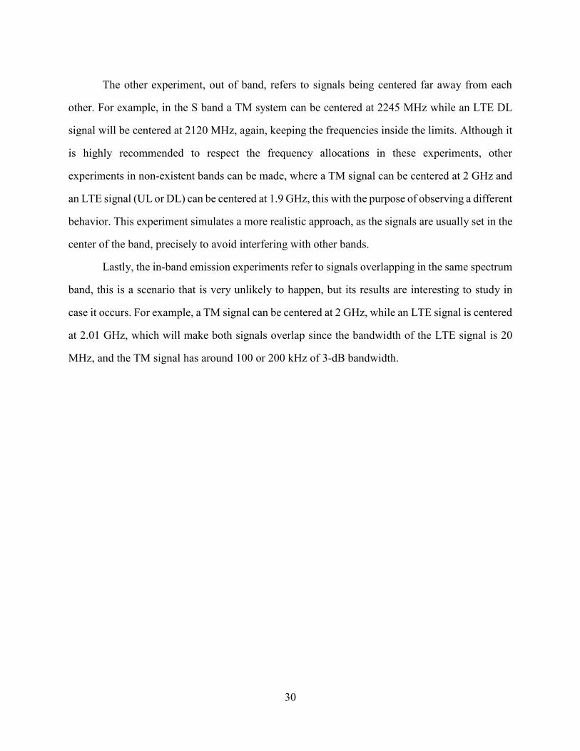
conditions are met, and no interference is present. Figure 5.1 displays the spectrum of a clean LTE

Downlink (DL) signal, no other signal is overlapping it and its square flat shape can be easily

distinguished. This signal is sent from the eNB station to the UE device.

32

Figure 5.1: LTE DL OFDM Carrier with no interference.

For the receiver side, more results are available, and these aid in determining the quality of

the link from the UE to the eNB station, this link is known as the LTE Uplink (UL). Figure 5.2

displays a clean signal from the UE device to the eNB station, its shape is clearly distinguishable

even though there are harmonics seen in the figure. These unwanted harmonics are produced by

the local oscillator of the SDR device.

Figure 5.3 gives the quantified values of the Physical Uplink Shared Channel (PUSCH)

which are throughput, in which the greater the number the better the quality of the link, and the

Block Error Rate (BLER) which is desired to be as close to zero as possible.

33

Figure 5.2: The received signal from the UE to the eNB station.

Figure 5.3: Throughput and BLER for a clean UL signal.

Figure 5.4 is additional visual parameter that can aid in determining the quality of the link.

The BLER is desired to be zero, but in an ideal situation and taking into consideration that the Tx

power of an actual UE device is much smaller than that of an eNB station, certain losses are

expected. The constellation diagram is a great visual tool to determine the quality of a link as well

as seen in Figure 5.5, where the “dots” or sampling instants have to be as tight and close as possible.

If there were to be jitter induced in these dots, they would be noticeably scattered.

34

Figure 5.4: Plot of the BLER over time.

Figure 5.5: Constellation Diagram of a QPSK UL channel.

These visual and numerical parameters will be used as a baseline to compare further

experiments. It will be explained how one result is compared to the other, and why one is preferred

over the other.

35

5.1.2 LTE Uplink (UE device to eNB station)

As the DL channel, the UL channel also has several visual and numerical parameters that

aid in determining the quality of a link. As mentioned before, these images and numerical values

will represent the baseline (reference point) for further experiments. The spectrum of the

transmitted signal from the UE to the eNB station is clearly seen in Figure 5.6 where there is no

interference. Notice that the main lobe or the peaks of the signal are not centered at 1.8 GHz even

though that is the center frequency at which it is transmitted. This is an LTE standard in which the

signal, if demodulated correctly, will show a frequency offset error of 7.5 kHz [18].

Figure 5.6: Transmitted LTE UL channel signal.

5.1.3 Telemetry Baseline Characteristics

Two tests were ran to baseline the TM system with a BPSK and an OQPSK signal. These

tests were run with a clean PSK modulated signal, meaning that no interference from the LTE

system was present. The presets for the TM system both had these characteristics:

• Tx Gain: 10 dB

• Rx Gain: 10 dB

• Center Frequency: 1.8 GHz

• Modulation Scheme: BPSK, QPSK, and OQPSK

36

This test was simply comprised of a Tx and Rx pair in a closed controlled system. There

was only one channel or link as compared to the two of the LTE system. Figure 5.7 is a clean

BPSK carrier centered at 1.8 GHz, the apparent power transmitted is close to -35 dBm. This will

be used as a point of comparison when other signals are sent, although the Tx signal is usually not

interfered, while the Rx signal is where the losses of the cable and the splitters are seen. From this,

a constellation diagram is also obtained as seen in Figure 5.8, the constellation diagram represents

the signal in a two-dimensional scatter diagram. The dots represent the possible symbols that may

be selected by a given modulation scheme as points in the complex plane [19].

Figure 5.7: A clean BPSK transmitted signal with a 150 kHz bandwidth.

37

Figure 5.8: BPSK constellation rotated 90 degrees.

The last element to be obtained is the eye diagram from the transmitter as seen in Figure

5.9. The eye diagram is used to determine the effects of channel noise and intersymbol interference.

The SNR can be determined by the opening of the eye, and in the following tests, a noisier channel

will be studied, and the effects on the eye diagram will be easy to see.

Figure 5.9: Eye diagram of a clean BPSK signal.

38

The previous visual parameters are useful in determining the quality of a Tx link, whenever

the Rx visual parameters are equal (in theory) to the ones presented before, it can be inferred that

the link quality is acceptable.

To compare these parameters, images taken from the testbed were obtained for the

receiving side. A spectrum graph was obtain as seen in Figure 5.10, where it is clearly seen that

some induced noise was present, although, it is safe to say that this signal is of good quality; the

baseline signal will be compared to the ones in the test to determine how much noise was induced.

It is also worth mentioning that the power transmitted was reduced by 15 dBm, it can be increased

if desired by using the amplifier, but with this baseline test it was sufficient and the amplifier was

not required.

Figure 5.10: The received BPSK signal.

The second visual parameter that can be obtained and compared is the constellation

diagram. In Figure 5.11 the Rx constellation diagram is shown, and it is clearly seen that it does

not look similar to the Tx constellation diagram. Noise was induced along the path of the wave,

but it is still easy to notice that it is still the same BPSK constellation. Other modulation schemes

produce different eye diagrams that will be shown for further reference, although, the two

modulation schemes used for telemetry are BPSK, and OQPSK.

39

Figure 5.11: Received BPSK constellation diagram.

These parameters can also be compared with the eye diagram. The three visual parameters

transmitted are received, and it is helpful in such a way that the user can see how the

communication link behaves under specific conditions. In Error! Reference source not found. the

shape of the eye diagram is clearly seen, and it can be determined that it looks very similar to the

one presented in the Tx counterpart. Although, some noise which is expected is included in the

link, making the eye diagram look “fuzzy”.

Figure 5.12: The Rx 2-length eye diagram for a BPSK signal.

40

The purpose of using two modulation schemes for the TM system is to observe how they

behave in different scenarios. In BPSK, there is only one bit per symbol, while in OQPSK there

are two bits per symbol, which means that the data rate of an OQPSK signal is double than that of

a BPSK signal while conserving the same bandwidth. In Figure 5.13, the constellation diagram of

an OQPSK signal is shown, and it is clearly seen that the constellation varies with respect to the

BPSK signal. Also, in Figure 5.14, the received constellation diagram is shown with the purpose

of comparing it to the transmitted constellation.

Figure 5.13: Tx constellation diagram of an OQPSK signal.

41

Figure 5.14: Rx constellation diagram for an OQPSK signal.

It can be clearly seen that some noise has been induced in the channel, although, this noise

is minimal compared to the noise that will be seen in the interference scenarios. Finally, the FSER

for a QPSK and BPSK signal was obtained, for the OQPSK signal, a preliminary FSER was

calculated. This FSER is still under work since there are some settings that have to be adjusted.

5.2 TELEMETRY INTERFERENCE ON LTE SYSTEMS

The first tests ran were done in order to answer the question of how much can the TM

system impact an LTE system. It is important to note that the TM interference is more significant

on commercial users, as its interference is noticeable and may prevent LTE service.

Both lower and upper band visual measurements were obtained. These visual

measurements represent how much a TM signal affects an LTE signal. The first images depict an

ideal scenario with no interference, which will be used as the reference or baseline.

For the interference tests, the Agilent (now Keysight) spectrum analyzer was used to

capture the spectrum when both TM and LTE signals were transmitted. The testbed was used to

acquire the images that aid in the quantification and qualification of the link.

42

5.2.1 Lower L-band

The first experiment was conducted on lower L-band frequencies. Note that the LTE

frequencies are made up and the TM frequencies are inside the frequencies regulated by the IRIG-

106 document. Some of the tests might include the actual carriers inside regulated frequency

bands, and since it is a controlled closed system, there is no risk of FCC rule violations.

Equal power levels output by the TM and LTE systems

As mentioned before, the adjacent band test is of utmost interest. In this case, a TM signal

was generated with the following characteristics:

• Modulation Scheme: OQPSK with 100 kHz of 3-dB bandwidth.


• Tx Gain/Tx Power: 5 dB

And an LTE DL signal was generated with the following characteristics:

• DL

o Modulation Scheme: MCS 17 (64-QAM)

o Center Frequency: 1.470 GHz

o Tx Power: 20 dBm

In this experiment, the same power level was transmitted for both signals. This test

represents the closest the signals can be without the LTE suffering from interference. The graph

in Figure 5.15 represents them in the radio spectrum. With these conditions, the LTE system

behaves normally, as seen in Figure 5.16 where the BLER remained at zero. With Figure 5.17, it

can be reinforced that this configuration of the TM signal does not affect the LTE system.

43

Figure 5.15: OQPSK TM signal and LTE DL signal in adjacent bands. The center frequency is

1.445 GHz.

Figure 5.16: BLER for the LTE system.

44

Figure 5.17: Constellation, data rate over time, and throughput for the LTE system.

The following test was made to determine how much a TM signal can affect an LTE signal

in an in-band scenario. In this case, the TM signal was centered at 1.46 GHz while the LTE signal

stayed at 1.47 GHz. This signals can be seen together in Figure 5.18 and the BLER measurement

is seen in Figure 5.19, lastly more measurements can be seen in Figure 5.20 where the data rate

has decreased by 33% on average due to the interference of the TM system.

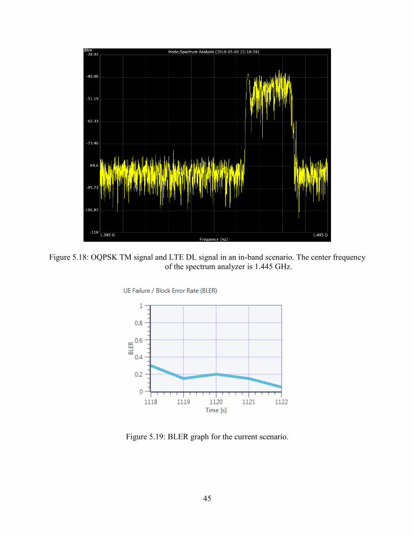
45

Figure 5.18: OQPSK TM signal and LTE DL signal in an in-band scenario. The center frequency

of the spectrum analyzer is 1.445 GHz.

Figure 5.19: BLER graph for the current scenario.

46

Figure 5.20: More measurements for the LTE system.

The final test on the lower L-band for TM interference on LTE was performed where both

systems were transmitting at a center frequency of 1.45 GHz. If both systems are transmitting at

the same center frequency, then the LTE suffers greatly from this interference as seen in the

following figures.

In Figure 5.21, the spectrum graph shows both signals overlapping, the LTE signal can be

seen with the TM signal in the middle, but both are hard to distinguish. The BLER in Figure 5.22

displays how much the LTE system was impacted, almost to the point of being unable to operate.

Lastly, Figure 5.23 depicts the performance drop in the DL of the LTE system.

47

Figure 5.21: Both TM and LTE signals overlapping.

Figure 5.22: BLER for the LTE system with the TM overlapped signal.

48

Figure 5.23: Constellation graph and data rate drop as well as throughput for the LTE system.

TM power increased above the LTE power level

By doubling the Tx gain in the TM system from 5 dB to 10 dB with a 20 MHz separation

(1.43 GHz for TM and 1.45 GHz for LTE), the behavior between systems becomes different as

described before. The separation between signals becomes shorter now that the power has

increased, in Figure 5.24 it is clearly seen that both signals are far from each other and can function

normally. In Figure 5.25 and Figure 5.26 the parameters to determine the quality of the LTE system

can be observed, and it is determined that the link was not affected by this scenario.

49

Figure 5.24: Spectrum graph of the two signals, with the TM system having more power than the

LTE signal.

Figure 5.25: BLER of the scenario.

50

Figure 5.26: More parameters to qualify and quantify the scenario.

The experiment where interference is beginning to affect the LTE system is when the TM

signal is separated by a value lower than 20 MHz. This is where the interference begins to affect

the LTE system considerably. Figure 5.27 displays the effects of this scenario, where the TM signal

is close to the LTE signal, which are 15 MHz apart. Also, the BLER is displayed in the same

figure, and it can be inferred that the system is affected considerably. Finally, Figure 5.28 makes

it easy to see how the system was affected by looking into the additional parameters provided.

From these results, it was determined that any gain above 10 dB (or -45 dBm) for the TM

system will behave in a similar fashion to a gain at the 10 dB level. Hence, why the results were

not included.

51

Figure 5.27: Spectrum graph and BLER graph for the described scenario.

Figure 5.28: Additional parameters for qualification and quantification of the scenario.

5.2.2 Upper L-band

The same experiments that were run in the lower L-band will be run in the upper L-band

to study the possibility of the systems not behaving the same in different frequencies. In wireless

systems, it is expected that the propagation loss is higher at higher frequencies, but in closed

controlled systems this might not be the case.

52

For these experiments, the TM and LTE DL systems will be operating in the 1710 – 1850

MHz frequency band. The first experiment will consist of a TM signal transmitting in an out of

band fashion relative to the LTE system, and for the further tests, the TM signal will be getting

closer to the LTE signal, in which the behavior will be recorded.


The first test consisted of the TM and LTE signals being transmitted at the same power

level (5 dB gain for the TM Tx and 20 dBm for the LTE Tx) transmitting at different frequencies.

The modulation schemes remain the same for the tests as well.

• TM center frequency at 1.8 GHz.

• LTE DL center frequency at 1.82 GHz.

With a 20 MHz separation, the following results were found, and in Figure 5.29 the

spectrum graph where the two signals are displayed as well as the BLER graph are shown, where

the BLER remains at zero which is desirably. This signifies that the LTE system was not affected

by the configuration of the TM signal.

Figure 5.29: Spectrum and BLER graph for the current scenario. The spectrum analyzer was

centered at 1.8 GHz.

53

Figure 5.30: Additional qualification and quantification parameters for the scenario.

Figure 5.30 complements the fact that the system was not affected. The data rate remained

constant while the constellation dots seem very tight together. Referring to the fact of the lower L-

band experiments where a 20 MHz band at the same power level is safe.

Continuing the experimentation, the TM signal will conserve the same gain/power and it

will get closer to the LTE signal in order to study its behavior. In this experiment, the TM signal

will be centered at 1.805 GHz to have a 15 MHz separation. The LTE system will remain in the

same configuration. In Figure 5.31 it is clearly seen that the LTE system was not disturbed despite

the distance between the signals, and in Figure 5.32 it is reinforced that the TM signal is not

affecting the LTE system. With these parameters, it is easy to determine that the TM link is not

affecting the LTE link as long as it stays at a distance of 15 MHz, while at the same power level.

This could be classified as the guard band distance.

54

Figure 5.31: Spectrum and BLER graphs for the current configuration. No interference detected.

Figure 5.32: Additional parameters for the LTE system. No detrimental interference observed.

The following experiment was done in order to determine that at any separation lower than

15 MHz is when the LTE system begins to reduce its performance. Figure 5.33 shows that the

signals in the spectrum are almost merging, and that the BLER beings to vary. This BLER means

that some error will be induced in the system due to the interference. There is one important thing

to notice, in Figure 5.34, the constellation remains tight but the throughput decreases; it does not

decrease by a large amount, but it is still considered a decrease compared to the baseline.

55

Figure 5.33: Spectrum and BLER graph for the current scenario. BLER starts to vary.

Figure 5.34: More performance metrics, the throughput does not see much of a change.


The following experiment consists of the TM gain being increased to corroborate with the

fact that a 20 MHz guard band is enough when the TM power is greater than the LTE power. The

TM gain will be increased to 15 dB and the LTE system will remain the same. The starting center

56

frequency for the TM system will be 1.8 GHz and the LTE system will remain at 1.82 GHz. The

TM signal will get closer in order to determine at what distance the LTE system will be affected.

Figure 5.35: Spectrum and BLER graphs for the current experiment.

Figure 5.36: Constellation and data rate parameters for the current experiment.

With the TM signal closer to the LTE signal, conserving the same configuration, a different

behavior was observed when they were 15 MHz apart. In Figure 5.37, the spectrum graph shows

that the signals are easily distinguishable, but the BLER graph shows that the errors are very

considerable, up to the point of the LTE link being inoperable for most of the time. To corroborate

these results, Figure 5.38 shows how degraded the link became with the TM signal. The

57

constellation is barely recognizable, and the data rate and throughput have been reduced by almost

95%. This reinforces the rule that at higher power, a band guard of 20 MHz is necessary.

Figure 5.37: Spectrum and BLER graphs for the current experiment.

Figure 5.38: Constellation diagram, data rate graph, and throughput metrics.

This concludes the experiments done on the L-band. It was observed how from the lower

L to the upper L-band had different behavior when the TM system was set to a higher power than

that of the LTE system. The next experiments will focus on the S-band, and lastly, the C-band

where the effects of higher frequencies will be studied.

58

5.2.3 Lower S-band

The following experiments will be conducted in the lower S-band which is at higher

frequencies than the L-band. Theoretically, in a wireless system, at higher frequencies the path

loss is higher, but in this experiment the effects will be studied in a closed controlled system.


The first tests consisted of the following parameters:

• TM

o Modulation Scheme: OQPSK with 100 kHz of 3-dB bandwidth


o Tx Gain: 5 dB

• LTE DL



o Tx Power: 20 dBm

Once again, the signals will be separated by 20 MHz to see how the systems behave. If

there is any interference that might affect the system, the measurements will display them. Figure

5.39 and Figure 5.40 prove that this configuration does not affect the LTE system at all. The LTE

system can function normally at this state.

59

Figure 5.39: Spectrum and the LTE BLER graph of the current experiment.

Figure 5.40: Additional metrics for measuring the LTE performance.

The following experiment will test the behavior of the TM and LTE systems 15 MHz apart

to determine if the link is still operable, and to observe how much is the quality of the LTE system

affected (if any). The power level for both systems remain the same, and the center frequency of

the TM signal is shifted to 2.205 GHz. Figure 5.41 and Figure 5.42 prove that there are no

noticeable changes or detrimental effects on the LTE system due to the TM signal. Once again,

this proves that the 15 MHz guard band is more than enough at the same power level.

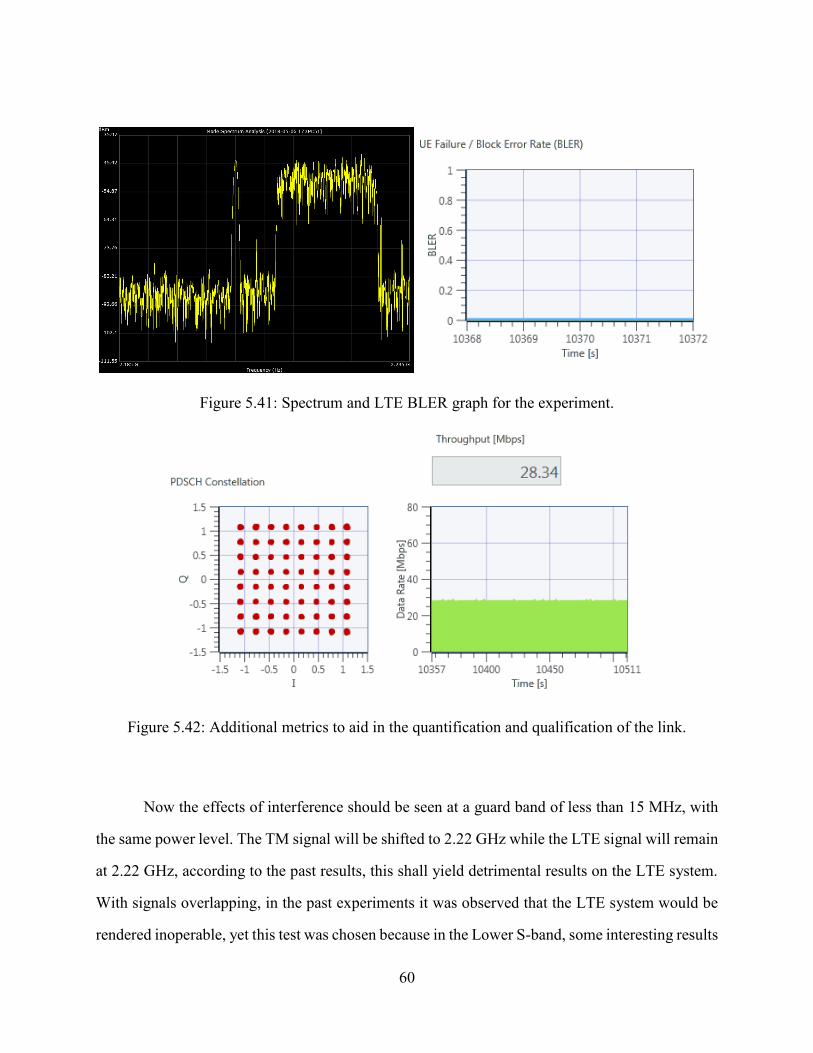
60

Figure 5.41: Spectrum and LTE BLER graph for the experiment.

Figure 5.42: Additional metrics to aid in the quantification and qualification of the link.

Now the effects of interference should be seen at a guard band of less than 15 MHz, with

the same power level. The TM signal will be shifted to 2.22 GHz while the LTE signal will remain

at 2.22 GHz, according to the past results, this shall yield detrimental results on the LTE system.

With signals overlapping, in the past experiments it was observed that the LTE system would be

rendered inoperable, yet this test was chosen because in the Lower S-band, some interesting results

61

were found out. In Figure 5.43, it is clearly seen that the TM signal is completely lost inside the

LTE signal, and, the BLER of the LTE system was very minimal to what was expected compared

to the other results. In the lower L-band, the same experiment rendered the LTE system inoperable,

while on this test in the lower S-band, the LTE system functions perfectly. Figure 5.44 further

reinforces the fact that the LTE system was not affected by the TM signal, which means that at the

same power level, the TM signal does not affect the LTE system at all in the lower S-band.

Although, it can be said that there are minor decreases in performance, but not so large to affect

the LTE system considerably.

Figure 5.43: The spectrum graph shows both signals overlapping, and the LTE BLER shows the

result of this.

62

Figure 5.44: Additional parameters that show that the LTE link is still in decent operation.


After the overlapping experiment made no significant interference, a higher power level

will be injected to the TM signal to prove if it yields the same results. In this scenario, the TM

signal will be shifted to the 2.23 GHz and the LTE system will be at 2.25 GHz. The TM signal’s

gain was increased to 15 dB from 5 dB in order to try to interfere with the LTE system. Again, it

is proven that at higher power levels, a 20 MHz is more than enough as seen in Figure 5.45. Also,

Figure 5.46 further contributes to this statement.

63

Figure 5.45: Spectrum graph and the LTE BLER graph for the current scenario.

Figure 5.46: The parameters obtained here reinforce the figure above.

For the following experiment, the TM signal was shifted to the 2.235 GHz frequency, while

the LTE remained the same, for this scenario, a guard band of 15 MHz was studied to determine

if it kept the LTE system running at an acceptable performance. For the same power level test,

there were no noticeable interference issues, could be to the fact that the LTE signal completely

overshadowed the TM signal. Although, in this test a different result was obtained, such as in

Figure 5.47 where the graph shows that the signals are at 15 MHz from each other, and the BLER

graph shows that the errors started to increase due to this. Again, reinforcing the idea that the TM

64

and LTE signals should be at least 20 MHz apart from each other to avoid interference. To further

contribute to this statement, Figure 5.48 shows that there is a 33% reduction in performance,

meaning that in fact, the TM system affected the LTE system greatly.

Figure 5.47: Spectrum graph for the TM and LTE signals and BLER graph for the LTE system.

Figure 5.48: Constellation diagram and data rate graph for the LTE system.

These results conclude the experimentation on the lower S-band, it was interesting to

discover that the TM system did not affect the LTE system while remaining at the same power

65

level, although when the TM system increases power, it follows the same rule of the 20 MHz guard

band requirement.

The following experiments will be conducted in the upper S-band, and the behavior will

be recorded as well to determine if the same rules apply to these scenarios.

5.2.4 Upper S-band

The same experiments will now be shifted into the upper S-band. The same rules will be

tested here such as 15 MHz guard band required for the same power level and 20 MHz required

for the TM signal with higher power. Similar results are expected, although there can be a situation

where the rule does not apply.


The first tests consist of the following:

• TM



o Tx Gain: 5 dB

• LTE DL



o Tx Power: 20 dBm

The results of the configuration described before are presented in Figure 5.49 and Figure

5.50, which clearly depict that the LTE system was not affected by the TM signal. Although it is

important to notice that the constellation graph has a small amount of jitter, which could mean that

getting the TM signal closer will induce errors.

66

Figure 5.49: Spectrum graph of the signals, and BLER of the LTE system.

Figure 5.50: Constellation and data rate graphs.

This next experiment was performed to determine if the LTE system will still function

while the TM signal was overlapping, to see if the same behavior from the lower S-band is

observed in the upper S-band. The results obtained were interesting, and Figure 5.51 proves the

same behavior. While the TM signal is completely in-band of the LTE signal, there is no noticeable

interference for the system, as the BLER graph shows. Figure 5.52 also proves that there were no

detrimental effects on the LTE system despite the TM signal being right in the middle.

67

Figure 5.51: Both TM and LTE signals overlapping in the spectrum graph while the LTE BLER

remains at zero.

Figure 5.52: Jittery constellation graph and constant data rate.


The following experiments will consist of increasing the TM signal gain to 15 dB from 5

dB. As observed in the lower S-band, it is expected to conserve the same behavior. With a greater

68

power transmitted from the TM system, the LTE system is expected to deteriorate when the signals

are less than 20 MHz apart.

The test will resort back to the first configuration of the first experiment done on the upper

S-band, while only varying in the gain of the TM Tx. To begin, the signals will be 20 MHz apart

as shown in the spectrum graph of Figure 5.53, also the BLER of the LTE system is shown in this

figure, and it proves that at 20 MHz apart, the LTE system works normally. To strengthen this

claim, Figure 5.54 displays that the values obtained from this experiment are similar to the baseline

values.

Figure 5.53: Spectrum graph and LTE BLER graphs for the current experiment.

69

Figure 5.54: Additional parameters that prove the LTE system works normally.

In past tests, the LTE system would begin to suffer from interference when the signals were

15 MHz apart, hence, in the following test a similar procedure will be experimented.

The TM frequency will be shifted up to 2.37 GHz in order to be 15 MHz apart from the

LTE signal. Figure 5.55 shows that the BLER curve is not at zero, hence, some errors will be

induced into the system. Figure 5.56 further explores the degradation of the LTE system due to

interference from the TM source. Reasserting again that a minimum distance of 20 MHz is required

between TM and LTE signals to conserve operation.

70

Figure 5.55: Spectrum graph of the two signals and LTE BLER graph.

Figure 5.56: These metrics show that the performance of the LTE system was degraded due to

the TM signal.

5.2.4 Lower C-band

The similar experiments conducted in the past bands will also be performed in the lower

C-band.

71


First, a TM signal will be transmitted to try to interfere with an LTE system with both

having the following initial characteristics:

• TM



o Tx Gain: 5 dB

• LTE DL



o Tx Power: 20 dBm

The first test will be run with the frequencies 15 MHz apart, since for the last tests, it has

been seen that 20 MHz is when the LTE system begins to throttle. Although, this effect only

happened in the L-band but not in the S-band, hence, it is important to repeat the scenario in the

C-bands.

In the C-band, a lot of losses are expected since it is an experiment in a high frequency

range. Hence the result of the none-interfered baseline test for the C-band yielded the results in

Figure 5.57, which shows that there is significant loss due to the high frequency at which it is

operated. Also, Figure 5.58 shows that there are some errors despite no interference being present

in the system.

72

Figure 5.57: Spectrum graph and BLER for the LTE system with no TM interference.

Figure 5.58: Constellation and data rate.

After acquiring the baseline values for the LTE system at high frequencies, a TM signal

was inserted at 4.595 GHz, making it 20 MHz apart to test the band guard. And the results show

that this was enough to keep the LTE link operational as seen in Figure 5.59 where the values are

close to the baseline. Figure 5.60 further proves that this configuration remains within the values

of the lower C-band baseline values, and it is safe to assume that 20 MHz is an acceptable quantity

for a guard band.

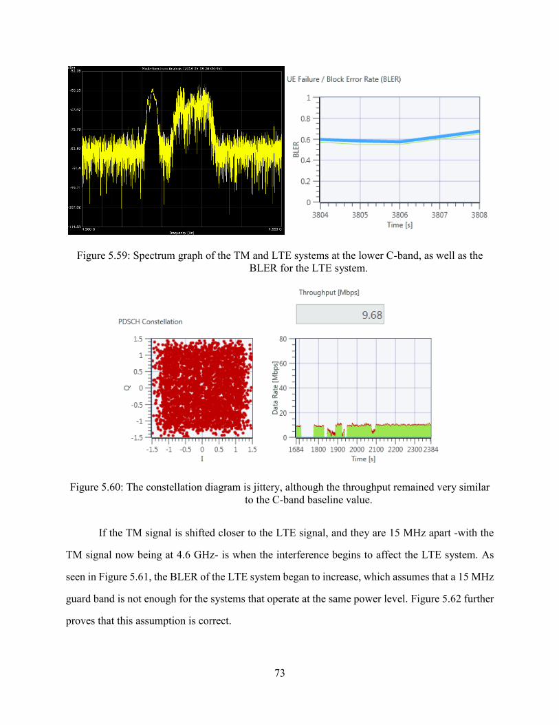
73

Figure 5.59: Spectrum graph of the TM and LTE systems at the lower C-band, as well as the

BLER for the LTE system.

Figure 5.60: The constellation diagram is jittery, although the throughput remained very similar

to the C-band baseline value.

If the TM signal is shifted closer to the LTE signal, and they are 15 MHz apart -with the

TM signal now being at 4.6 GHz- is when the interference begins to affect the LTE system. As

seen in Figure 5.61, the BLER of the LTE system began to increase, which assumes that a 15 MHz

guard band is not enough for the systems that operate at the same power level. Figure 5.62 further

proves that this assumption is correct.

74

Figure 5.61: Spectrum graph of the two signals 15 MHz apart, and the BLER of the LTE system

that indicates the interference was significant.

Figure 5.62: Constellation diagram and data rate for the LTE system.


When the TM signal overpowers the LTE signal, the 20 MHz guard band is still acceptable

to conserve an LTE system. Figure 5.63 shows the signal adjacent to each other, and shows the

BLER graph. While the BLER does not remain at zero, the link is still operational and has

sufficient throughput as seen in

75

Figure 5.63: The spectrum graph shows that the TM signal overpowers the LTE signal by a small

factor, and the BLER graph shows that the link has some errors but remains

operational.

Figure 5.64: Constellation diagram and the data rate graph that shows the link is still operational.

In the past tests, it was observed that the LTE system was still operational under TM

interference, but when the TM signal overpowers the LTE signal and are at 15 MHz apart, the LTE

link is rendered useless. Figure 5.65 shows how the signals are very close to each other, and that

the BLER is at a value of one most of the time, rendering the link useless. Figure 5.66 shows how

the link is not operational under these conditions.

76

Figure 5.65: Spectrum graph of the semi-overlapping signals and the BLER at a high value.

Figure 5.66: Completely scattered and jittery constellation with a throughput of zero.

The experiments performed on the lower C-band proved that the conditions of the system

change drastically and that more caution has to be taken into consideration. Higher frequencies

behave in a very distinct manner in comparison to the lower frequency bands, hence why it is

advised to follow the rules presented herein to ensure an acceptable performance.

5.2.5 Middle C-band

Once again, the system is shifted to higher frequencies to observe the behavior. It is

expected that the LTE link will be degraded even when no interference is present. Both TM and

77

LTE systems suffer from the high frequencies, as seen in the spectrum graph of Figure 5.67 where

both have suffered major attenuation. Although, Figure 5.68 shows that the LTE link is still

operational with a reduced data rate.


Further experiments will emulate the conditions presented in the lower C-band

experiments, starting with the TM and LTE signals at the same power level, 20 MHz apart, and

then 15 MHz apart. This to observe and classify their behavior.

Figure 5.67: Spectrum graph of the signals and BLER graph of the TM system.

78

Figure 5.68: Clear constellation diagram and decent data rate for the LTE system.

The following experiment consists of the two signals at 15 MHz apart to see if the

degradation of the LTE system becomes greater. In this test, the same condition was proven as in

the lower C-band, that when the TM signal is 20 MHz or lower, the LTE system begins to suffer.

Figure 5.69 shows how the signals are together and how the BLER of the LTE system was affected.

Figure 5.70 shows how the link was affected and even though there are instances where the data

rate is high, on average, the data rate suffers from this interference.

Figure 5.69: Spectrum graph of the signals in the middle C-band and the affected BLER.

79

Figure 5.70: Clear constellation but low data rate and throughput.


From the results presented herein, a higher power TM signal will be tested in order to

corroborate the idea of a 20 MHz guard band. In this scenario, a TM signal will be centered at

5.115 GHz and it is expected to degrade the LTE system completely.

The results from the test show that a 20 MHz guard band is indeed necessary to conserve

the LTE system operational, even if it is at lower data rates. Figure 5.71 shows that the LTE link

was affected greatly since the BLER values are extremely high, which could lead to the LTE

system being inoperable. To further observe this case, Figure 5.72 shows that the link has been

degraded almost to the point of no operation. Even though there is still a very small data rate, the

end-user will most likely identify it as the link being inoperable. Again, strengthening the claims

stated before.

80

Figure 5.71: Spectrum graph and a high BLER for the LTE system.

Figure 5.72: Constellation diagram with a very low throughput graph.

With the TM on LTE interference scenarios presented in the L, S, and C-band, the

following tests will now include the interference of LTE on TM systems. A different behavior is

expected to rise, hence why the new experimentation is presented.

5.3 LTE INTERFERENCE ON TELEMETRY SYSTEMS

After testing how the TM signals will affect the LTE system, it is required to also study

how the LTE system would affect the TM system. With this, stricter rules of interaction can be

81

created for both systems in order to maximize coexistence. A similar approach to experimentation

as the previous section will be followed. A TM signal will be centered at a specific frequency

while the TM signal will be shifting closer in order to interfere with the TM signal. An OQPSK

signal will be used to test this scenario, the parameters that will help classify the TM system will

be the constellation diagram, spectrum graph from spectrum analyzer and testbed, eye diagram,

and a preliminary FSER graph.

Interfering with TM is not as severe as interfering with LTE, since the private companies

are spending large amounts of money to keep their links fully operational, and anyone who tampers

with them will be probably fined. Hence, why the TM on LTE interference issue was explored

first.

As the TM on LTE tests, this LTE on TM tests will be also conducted in the L, S, and C-

bands. The same spectrum analyzer will be utilized, while the other parameters will be extracted

from the TM transceiver GUI. Once again, the testbed was used to acquire the images that aid in

the quantification and qualification of the link.

These tests will mainly show that the TM signal works under LTE interference as long as

the TM signal overpowers the LTE signal. As mentioned before, the FSER value is still in a

preliminary state, which means that the FSER graph represents when the TM signal has actually

locked in to the synchronization bits (16 pseudo random bits) and that it is receiving those bits

correctly. The LTE is expected to break that sync at a certain power level above the TM system or

at a certain frequency.

5.3.1 Lower L-band

It is crucial to understand that the TM system is more resilient to the LTE system. This is

due to the fact that the LTE system is simply seen as noise to the TM system. Hence, the important

factor that would affect the TM system is the power of the LTE system, not so much the frequency

at which it is operating. And the results from the tests will be explained to fit this theory.

82

The first test performed was on the lower L-band. The TM frequencies will comply with

the standards set by the FCC, and the LTE frequencies will be made up in order to observe the

worst-case scenario to determine the best rules for the TM system. The reasoning behind finding

the worst-case scenario, is that any other scenario outside the worst-cases, will function normally

(in theory). As a result, all of the tests will be conducted as an in-band scenario and with the same

power level.

As mentioned before, the adjacent band test is of utmost interest. In this case, a TM signal

was generated with the following characteristics:

• Modulation Scheme: OQPSK with 200 kHz of 3-dB bandwidth.


• Tx Gain: 10 dB

• Rx Gain: 10 dB


• DL



o Tx Power: 20 dBm

This would make the signals 20 MHz apart, what will be studied is the noise increase on

the TM Rx due to the LTE signal. Once again, the 20 MHz bandwidth is good enough to conserve

the link of the TM system. Figure 5.73 shows how the signals are laid out in the spectrum while

the FSER shows that the link is still operational. From Figure 5.74, the qualification parameters

show us that the quality of the link is acceptable due to the constellation diagram being clear, as

well as the spectrum seen by the receiver, and the eye diagram of the receiver.

83

Figure 5.73: Spectrum of the TM and LTE signals 20 MHz apart. The FSER graph of the TM

system shows that the interference was not detrimental.

Figure 5.74: Additional parameters to qualify the OQPSK TM link. The constellation diagram,

spectrum received, and eye diagram.

The next test consisted of the LTE signal being shifted so that both signals were 10 MHz

apart. Meaning that the TM signal remained at 1.445 GHz and the LTE signal at 1.455 GHz. Since

the LTE signal has a bandwidth of 20 MHz, some overlapping may occur due to the short

separation. The spectrum graph in Figure 5.75 shows how the signals are almost merging, despite

being close to each other, the FSER remained at zero. One important factor that was observed can

be seen in Figure 5.76 is that the spectrum graph of the receiver noticed more noise in the system.

84

It can be inferred that the TM signal can be as close as 10 MHz to the LTE signal, but this

will affect the LTE greatly. The TM signal is more resilient to the LTE than the LTE being resilient

to TM.

Figure 5.75: Spectrum graph and FSER of the TM system.

Figure 5.76: Constellation diagram, spectrum graph with increased noise floor, and eye diagram.

This other experiment was done in order to observe what would happen when both signals

overlap, hence, both signals are now centered at 1.445 GHz. With this, it can be inferred that the

TM system will operate normally as long as the LTE signal does not overpower it. Figure 5.77

shows how the TM signal was completely hidden by the LTE signal, as seen by the spectrum

analyzer, and, the FSER had instances where a high value was obtained, rendering the system

85

useless. In Figure 5.78 it is clearly seen that the constellation diagram has lost its tightness, and

that the noise floor in the spectrum was increased by roughly 20 dBm. It is fair to mention that

these are theoretical values obtained by observing the spectrum graphs.

Figure 5.77: Overlapped signals and FSER graph that shows that at certain instances where the

FSER was 1.

Figure 5.78: Jittery constellation, spectrum graph, and eye diagram.

5.3.2 Upper L-band

Similar to the tests performed in the lower L-band, the experiments presented in this upper

L-band will follow a similar fashion. This to study the behavior of the TM system at different

86

frequencies and to characterize the interference the LTE system provokes by raising the noise floor

of the TM receiver.

For the first experiment, a TM signal was generated with the following characteristics:

• Modulation Scheme: OQPSK with 200 kHz of 3-dB bandwidth


• Tx Gain: 10 dB

• Rx Gain: 10 dB


• DL



o Tx Power: 20 dBm

With this configuration, the signals will be 15 MHz apart, and the impact of this scenario

will be studied. As seen in the past tests, the noise floor of the TM receiver was increased with no

noticeable issues. The spectrum graph in Figure 5.79 shows how the signals are next to each other,

and the FSER graph reasserts the assumption of the TM signal operating normally. The graphs in

Figure 5.80 show that the constellation diagram is in good shape, and that the noise floor was not

raised considerably on the TM system, while the eye diagram looks clear as well.

87

Figure 5.79: Spectrum graph and FSER.

Figure 5.80: Parameters seen by the TM receiver. Constellation diagram, spectrum graph, and

eye diagram.

The next test will have the two signals 5 MHz apart, which is an extreme case that in a real-

world scenario would not be possible due to the FCC regulations, but it has to be studied in order

to understand the scenario in case a mishap occurs. The LTE signal will be centered at 1.78 GHz,

while the TM signal will remain at 1.785 GHz. In Figure 5.81, the spectrum graph shows that there

is still a small amount of the TM signal shown, and that the FSER graph detected errors in the

system. In Figure 5.82, the constellation is sparse, the spectrum graph shows that a considerable

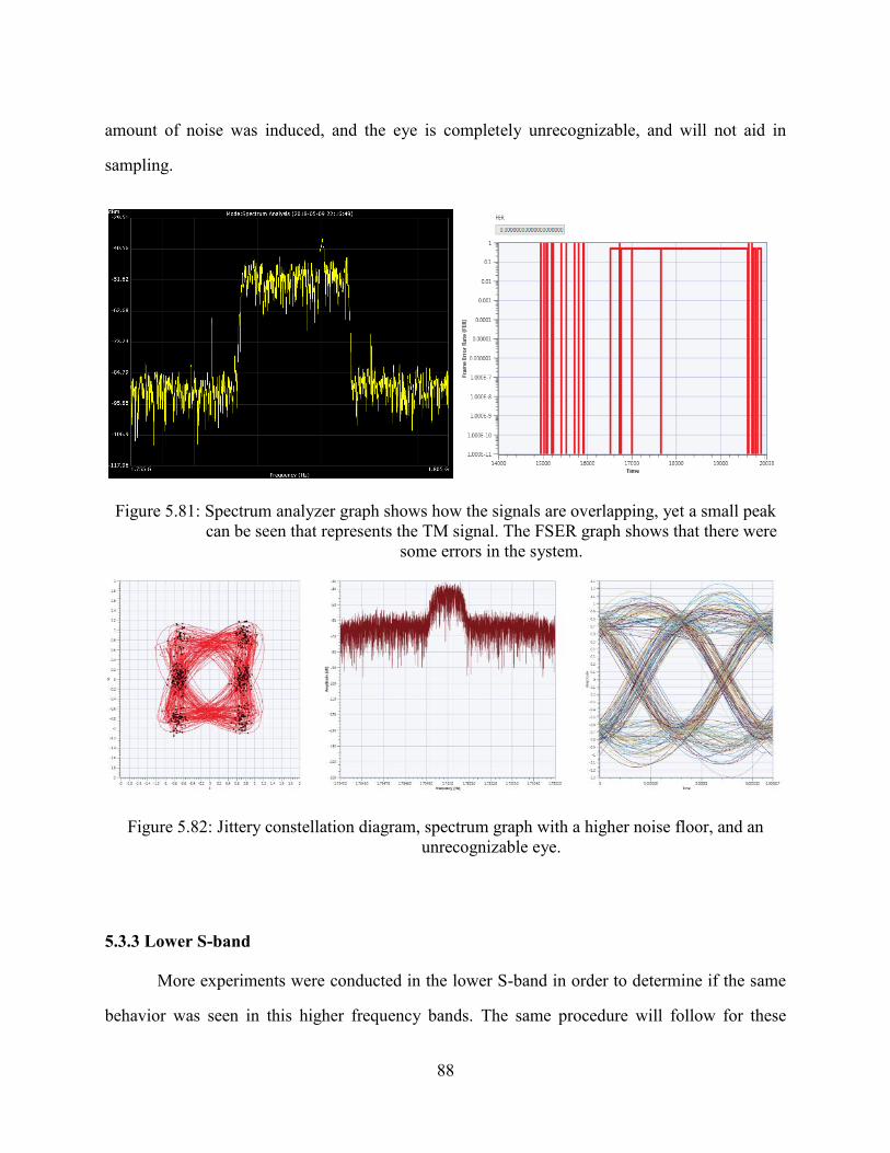
88

amount of noise was induced, and the eye is completely unrecognizable, and will not aid in

sampling.

Figure 5.81: Spectrum analyzer graph shows how the signals are overlapping, yet a small peak

can be seen that represents the TM signal. The FSER graph shows that there were

some errors in the system.

Figure 5.82: Jittery constellation diagram, spectrum graph with a higher noise floor, and an

unrecognizable eye.

5.3.3 Lower S-band

More experiments were conducted in the lower S-band in order to determine if the same

behavior was seen in this higher frequency bands. The same procedure will follow for these

89

experiments where the TM signal will remain centered and the LTE signal will be shifted among

the spectrum to reduce the guard band distance.

As previously mentioned, the frequencies will change but the system parameters will

remain the same, which are as follows:

• Modulation Scheme: OQPSK with 200 kHz of 3-dB bandwidth


• Tx Gain: 10 dB

• Rx Gain: 10 dB


• DL



o Tx Power: 20 dBm

The results from the experimentation reinforced the concept of how LTE interference

affects a TM system. With this 15 MHz distance, the following results were obtained as seen in

Figure 5.83, where the FSER plot remained at zero and the spectrum graph with both signals. To

further enhance this assumption, Figure 5.84 shows that the quality of the link is acceptable, as all

of the parameters are easily distinguishable. Again, this rule of the 15 MHz guard band proves that

it is enough to keep the TM link functioning.

90

Figure 5.83: Spectrum graph of the signals and FSER plot of the TM system.

Figure 5.84: Constellation diagram, spectrum graph as seen by the TM Rx, and eye diagram.

For this next test, the LTE signal will get closer in order to test the worst-case scenario,

when the LTE system will be transmitting in the TM band. The LTE signal will be 5 MHz apart

from the TM signal, hence, the TM signal will remain at 2.225 GHz, but the LTE signal will be

shifted down to 2.23 GHz. As expected, this scenario should affect the TM system greatly and

induce a high amount of errors. Again, it was proven that this scenario is greatly detrimental to the

TM system as seen in Figure 5.85 where the TM signal is almost hidden in the LTE signal, while

the FSER plot shows that many errors were present in the system. To reinforce this claim, the

graphs in Figure 5.86 show that the TM system became very jittery while the noise floor of the

91

spectrum graph was drastically increased, as well as rendering the eye diagram completely

unreadable.

Figure 5.85: Spectrum graph with the TM signal barely noticeable, and FSER plot of the system.

Figure 5.86: Qualitative graphs for the TM system with LTE interference.

5.3.3 Upper S-band

Moving to a higher frequency sees different behavior, although, it is expected that the

system functions similar to the lower S-band. Hence, the configuration for these scenarios is:

• Modulation Scheme: OQPSK with 200 kHz 3-dB bandwidth


92

• Tx Gain: 10 dB

• Rx Gain: 10 dB


• DL



o Tx Power: 20 dBm

The initial results obtained are displayed in Figure 5.87, where the spectrum graph is

showing both signals clearly, and the FSER graph remained at zero, meaning that a full sync was

obtained. Also, the visual parameters in Figure 5.88 demonstrate that the link is under normal

operation.

Figure 5.87: TM and LTE signals together. Spectrum graph and FSER.

93

Figure 5.88: Constellation diagram, TM Rx spectrum graph, and eye diagram.

The following test will encompass a center frequency separation of 10 MHz between

signals, again, in order to classify the LTE effect on the TM system. The power levels and

bandwidth will stay the same, but the center frequency of the LTE system will be shifted to 2.38

GHz. As seen in the resulting graphs of Figure 5.89, the TM signal is beginning to merge with the

LTE signal, which leads to the FSER graph in which several synchronization errors were found.

Figure 5.89: Spectrum graph and FSER for the TM system.

94

Figure 5.90: Jittery constellation, spectrum as seen by the TM Rx, and eye diagram.

With these results, it can be concluded that the LTE interference over the TM system

behaves in similar fashion in the L and S frequency bands. Again, reinforcing the idea that the

LTE interference on the TM system is seen as increasing the noise in the channel.

With a 15 MHz separation in the center frequencies, the TM link is still operational

although certain errors may be introduced. Small errors, but they will still be present. Although

the TM signal can be more resilient to LTE interference, it is still recommended to keep the 20

MHz guard band between center frequencies to ensure both systems remain operational.

5.3.4 Lower C-band

At higher frequencies, the system has been observed to struggle and in the following tests,

the performance degradation of working at higher frequencies as well as the LTE interference will

be observed.

It is important to baseline the system at the C-band frequencies, hence the graphs contained

in Figure 5.91 and Figure 5.92 show how the TM system operates normally at these high

frequencies.

95

Figure 5.91: Spectrum graph of the TM system at a lower C-band frequency.

Figure 5.92: Additional visual parameters for the TM system at a high frequency.

The first scenario’s configuration is:


• Center Frequency: 4405 GHz

• Tx Gain: 10 dB

• Rx Gain: 10 dB


• DL


o Center Frequency: 4390 GHz

96

o Tx Power: 20 dBm

The results proved that the LTE signal in fact affected the TM signal considerably. Figure

5.93 shows that even though the TM system already had synchronization errors, the LTE system

increased the number of errors due to it being close to the TM system. Figure 5.94 also displays

how this interference affected the system.

Figure 5.93: Spectrum graph of the TM and LTE signals, and the FSER for the TM system.

Figure 5.94: Jittery constellation diagram, with noisy spectrum seen by the TM Rx, and eye

diagram.

In order to keep the TM system with the least amount of errors, a 25 MHz center frequency

separation is needed. Figure 5.95 shows that still errors were present, but not in the same amount

than with the LTE interference.

97

Figure 5.95: Spectrum graph with the signals 25 MHz apart, and a FSER graph for the TM system.

5.3.4 Middle C-band

The measurements in the C-band have room from improvement, yet these early simulations

give an idea of what challenges there are, and where to focus first to develop a fully functional

system in the C-band. Hence, the configuration for this system is:



• Tx Gain: 10 dB

• Rx Gain: 10 dB


• DL



o Tx Power: 20 dBm

Similar results to the past tests were found, and they are depicted in Figure 5.96, which

agrees to the assumption that the system itself being at high frequencies affects the TM system.

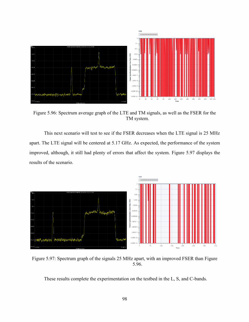
98

Figure 5.96: Spectrum average graph of the LTE and TM signals, as well as the FSER for the

TM system.

This next scenario will test to see if the FSER decreases when the LTE signal is 25 MHz

apart. The LTE signal will be centered at 5.17 GHz. As expected, the performance of the system

improved, although, it still had plenty of errors that affect the system. Figure 5.97 displays the

results of the scenario.

Figure 5.97: Spectrum graph of the signals 25 MHz apart, with an improved FSER than Figure

5.96.

These results complete the experimentation on the testbed in the L, S, and C-bands.

99

Chapter 6: Conclusions

This section includes the data of how the TM system affected the LTE system, their rules

of interaction in order to keep the LTE system at an acceptable performance, and a brief

introduction into how these results will aid in the 5G technologies by implementing a similar

testbed.

In the first cases of the interference of the TM system on the LTE system, it was clear that

there was a pattern developing for the L-band, from which two rules of interaction where obtained

to ensure the normal performance in an LTE system. The rules of interaction of an LTE and a TM

system in the L-band are as follows:

• If the TM and the LTE signals are at the same power level, to prevent interference

their minimum guard band distance should be no less than 15 MHz.

• If the TM signal overpowers the LTE signal, to avoid detrimental effects on the

LTE system, both signals should have a guard band distance of at least 20 MHz.

These rules were generated with the observations done on the results of the tests in the L-

band.

For the S-band, different results were yielded, which led to the suggestion of the following

rules to ensure normal operation for the LTE system.

• If the TM and the LTE signals are at the same power level, the LTE system will

suffer no considerable interference from the TM system. A small effect may be

observed on the LTE signal, but the TM system will be rendered useless if the

signals are overlapping or in close vicinity.

• If the TM signal overpowers the LTE signal, again, both signals should be spaced

at a minimum of 20 MHz to prevent interference on the LTE system.

The rules for the C-band change drastically, and according to the results, the LTE link

suffers from being operated at a high frequency even without interference; when interference is

introduced, the following rules can apply for the C-band:

100

• When the TM and the LTE systems display the same power level, a 20 MHz

distance between signals is needed to ensure the LTE system does not suffer any

additional degradation from the high frequency. The LTE link still functions but

with reduced performance.

• If the TM signal overpowers the LTE signal, a 20 MHz is also required to keep the

link operational. Any lower value of the band guard will render the LTE link

completely useless.

These rules of interaction conclude the TM on LTE interference scenarios. These rules are

strongly recommended to ensure normal performance of both systems and to make sure the signals

coexist harmoniously.

For the interference mitigation of the LTE system on the TM system, different rules must

be followed to protect the TM system. In the LTE system, interference from the TM system was

felt instantaneously and the performance of the link suffered greatly, the spectrum graph of the

LTE Rx displayed both TM and LTE signals simultaneously, and its effects were seen clearly. For

the TM system, the LTE signal remains masked as noise to the TM Rx, meaning that any LTE

signal that gets closer and closer to the TM signal, will only be raising the noise level of the TM

Rx, affecting its performance by increasing the FSER, reducing the channel capacity, and affecting

the visual parameters such as the constellation and eye diagrams.

As a result, for the TM system:

• Visual parameters should be taken into consideration when calculating/determining

the interference from the LTE system.

• The FSER measurements can be used as quantification for the quality of the TM

link.

• Following the rules established by the LTE rules of interaction should be followed

in order to prevent fines from the FCCEB.

• The TM system is resilient at the 15 MHz center frequency separation as long as

the power levels remain equal.

101

The 5G standard will include many technologies from the 4G standard, moreover, it will

be a collection of technologies that comprise 5G, not just a single one. 5G will pave the way for

the many Internet-of-Things (IoT) applications such as autonomous driving automobiles, big data

applications, personal devices, and more. With the inclusion of millimeter waves, small cells,

massive MIMO (Multiple-Input Multiple-Output), beamforming, and full duplex (Nordrum,

2017), a testbed concept can also be considered in order to test the possible scenarios that may

appear with the 5G technologies.

The 5G concept is still in development and many technologies have been suggested, and

the concept of building a testbed to experiment on the 5G scenarios is a possibility since the testbed

presented herein yielded results which aid in the rules of interaction between systems to ensure an

optimal performance. While the need for data increases, it is important to be prepared and

understand the limits of the communication systems, and with a developed testbed, it can be a

reality.

All the tests were conducted as worst-case scenarios in order to experiment with the limits

of the simulated systems. This to reduce the number of experiments required, since any other test

outside the worst-case scenarios is expected to function normally (in theory). With this flexible

SDR testbed, it was proven that the emulation of communication systems as well as their

qualification and quantification. This testbed focuses all the resources into the SDR which makes

it easy to manipulate via software.

102

References

[1] Federal Communications Commission (FCC), "Advanced Wireless Services (AWS),"

2017. [Online]. Available: https://www.fcc.gov/general/advanced-wireless-services-aws.

[2] J. Gonzalez, P. Rangel and V. Gonzalez, "White Sands Missile Range (WSMR) Radio

Spectrum Enterprise Testbed: A Spectrum Allocation Solution," The ITEA Journal, vol.

38, no. 2, pp. 159-163, June 2017.

[3] K. Temple, "An Initial Look at Adjacent Band Interference Between Aeronautical Mobile

Telemetry and Long-Term Evolution Wireless Service," California: Edwards Air Force

Base, 2016.

[4] M. Cotton and e. al., "An overview of the NTIA/NIST spectrum monitoring pilot

program,," in IEEE Wireless Communications and Networking Conference Workshops

(WCNCW), New Orleans, 2015.

[5] National Telecommunications and Information Administration, "United States Frequency

Allocations," 2016. [Online]. Available: https://www.ntia.doc.gov/page/2011/united-states-

frequency-allocation-chart.

[6] W.-B. Yang and M. Souryal, "LTE Physical Layer Performance Analysis," 2013.

[7] Quasonix, "Advanced Modulation Techniques for Telemetry," in International

Telemetering Conference, Las Vegas, 2011.

[8] Range Commanders Council, "IRIG Standard 106-17: Telemetry Standards," Secretariat

Range Commanders Council US Army, White Sands Missile Range, 2017.

[9] T. Tjelta and R. Struzak, "Spectrum Management Overview," The Radio Science Bulletin,

p. 28, March 2012.

[10] Z.-Q. Luo and S. Zhang, "Dynamic Spectrum Management: Complexity and Duality,"

IEEE Signal Processing Society, vol. 2, no. 1, pp. 57-73, 15 February 2008.

[11] Federal Communications Commission Internet Services Staff, "Enforcement Bureau,"

2015. [Online]. Available: http://transition.fcc.gov/eb/.

[12] 686_WG - Terminology Working Group, "IEEE Std 521-2002 (Revision of IEEE Std 521-

1984) - IEEE Standard Letter Designations for Radar-Frequency Bands," AES - IEEE

Aerospace and Electronic Systems Society, 2009.

[13] The Wireless Innovation Forum, "What is Software Defined Radio?," 2017. [Online].

Available: http://www.wirelessinnovation.org/Introduction_to_SDR.

[14] J. Polson, "Cognitive Radio Applications in Software Defined Radio," in SDR 04 Technical

Conference and Product Exposition, 2004.

[15] 3rd Generation Partnership Project (3GPP), "3rd Generation Partnership Project; Technical

Specification Group Radio Access Network; Evolved Universal Terrestrial Radio Access

103

(E-UTRA); User Equipment (UE) radio transmission and reception (Release 12)," 3GPP

TS 36.101, Valbonne - FRANCE, 2015.

[16] M. Reckeweg and C. Rohner, "Antenna Basics," Rhode & Schwarz, 2015.

[17] Adrio Communications Ltd, "LTE Frequency Bands & Spectrum Allocations," 6

November 2010. [Online]. Available: http://www.radio-

electronics.com/info/cellulartelecomms/lte-long-term-evolution/lte-frequency-

spectrum.php. [Accessed 9 November 2017].

[18] 3rd Generation Partnership Project (3GPP), "LTE; Evolved Universal Terrestrial Radio

Access (E-UTRA); Physical channels and modulation," 2008.

[19] A. S. Tanenbaum and D. J. Wetherall, "Digital Modulation and Multiplexing," in Computer

Networks, Pearson, 2010, pp. 131-132.

[20] K. Ghosh and A. Nath, "Cognitive Radio Networks: a comprehensive study on scope,"

International Journal of Innovative Research in Advanced Engineering (IJIRAE), vol. 2,

no. 12, pp. 44-56, December 2015.

[21] 3rd Generation Partnership Project, "Evolved Universal Terrestrial Radio Access (E-

UTRA) User Equipment (UE) radio transmission and reception," 3GPP Organizational

Partners' Publications Office, 2015.

[22] A. Nordrum, "Everything You Need to Know About 5G," 27 January 2017. [Online].

Available: https://spectrum.ieee.org/video/telecom/wireless/everything-you-need-to-know-

about-5g.

104

Glossary

3GPP 3rd Generation Partnership Project

4G Fourth generation of cellular technology (preceded by 3G).

AMT Aeronautical Mobile Telemetry

AWGN Additive White Gaussian Noise

BER Bit Error Rate

BLER Block Error Rate (4G LTE only)

BPSK Binary Phase-Shift Keying

BW Bandwidth

DL LTE-Downlink channel (from antenna to cellphone)

eNB eNodeB (cell tower)

FCC Federal Communications Commission

FER Frame Error Rate

FSER Frame Synchronization Error Rate

G/t Antenna Gain

I/Q In-phase/Quadrature components

IoT Internet-of-Things

ISM Industrial, Scientific, Medical radio frequency band

LHC Left Hand Circular Polarization

LTE Long Term Evolution

NF Noise Floor

NTIA National Telecommunications and Information Administration

105

OFDM Orthogonal Frequency-Division Multiplexing

OQPSK Offset Quadrature Phase-Shift Keying

PDSCH Physical Downlink Shared Channel

PSK Phase-Shift Keying

PUSCH Physical Uplink Shared Channel

QAM Quadrature Amplitude Modulation

QPSK Quadrature Phase-Shift Keying

RHC Right Hand Circular Polarization

Rx Receiver

SNR Signal-to-Noise Ratio

TM Telemetry

Tx Transmitter

UE User Equipment (cellphone, tablet, mobile device)

UL LTE-Uplink channel (from cellphone to antenna)

WSMR White Sands Missile Range

106

Vita

Juan Francisco González Flores was born on September 26, 1994. The third child of

Francisco Javier González Cázares and María del Rocío Flores Licón. He entered The University

of Texas at El Paso (UTEP) in the fall of 2012. While pursuing his bachelor's degree in Electrical

and Engineering, he worked for a year and a half as the assistant System Administrator in the

Electrical and Computer Engineering Department along with Rene Brito, under the command of

Nito Gumataotao. While working as a system admin, he did voluntary undergraduate research in

Fiber Optics with Dr. Joel Quintana; he won the 3rd place in the poster competition of the MAES

Symposium in October 2015. After terminating his system admin job, he went to work for one

semester in the Office of Technology Commercialization (OTC), a branch of the Office of

Research and Sponsored Projects (ORSP) at the University; where they specialized in

commercializing UTEP's inventions, for the inventors to sell and license their technology. He

received his Bachelor of Science in Electrical Engineering on May 2016. During the summer of

2016, he worked as an Environmental Engineering Intern under the supervision of Rajesh Bhakta;

where he focused on air quality systems and permitting.

He began his graduate studies at UTEP in the fall of 2016 to pursue his master’s degree in

electrical engineering. He worked as a Research Assistant under the supervision of Dr. Virgilio

Gonzalez, in the Cyberphysical Systems Laboratory, concentrating in the Applied

Communications section. He was able to continue pursuing education thanks to the funding of the

WSMR project conducted by Drs. Virgilio Gonzalez and Pablo Rangel; and thanks to the Texas

Instruments Foundation Endowed Scholarship in Spring 2016, Fall 2016, and Spring 2017. His

community involvement includes being the Vice President for the honor society of IEEE (IEEE-

HKN Zeta Delta chapter), the webmaster for MAES/SHPE and TSPE UTEP chapters, and as the

graduate adviser in UTEP's IEEE chapter.

This thesis was typed by Juan Francisco González.

Documents

Interference Analysis And Mitigation Of Telemetry (tm) And