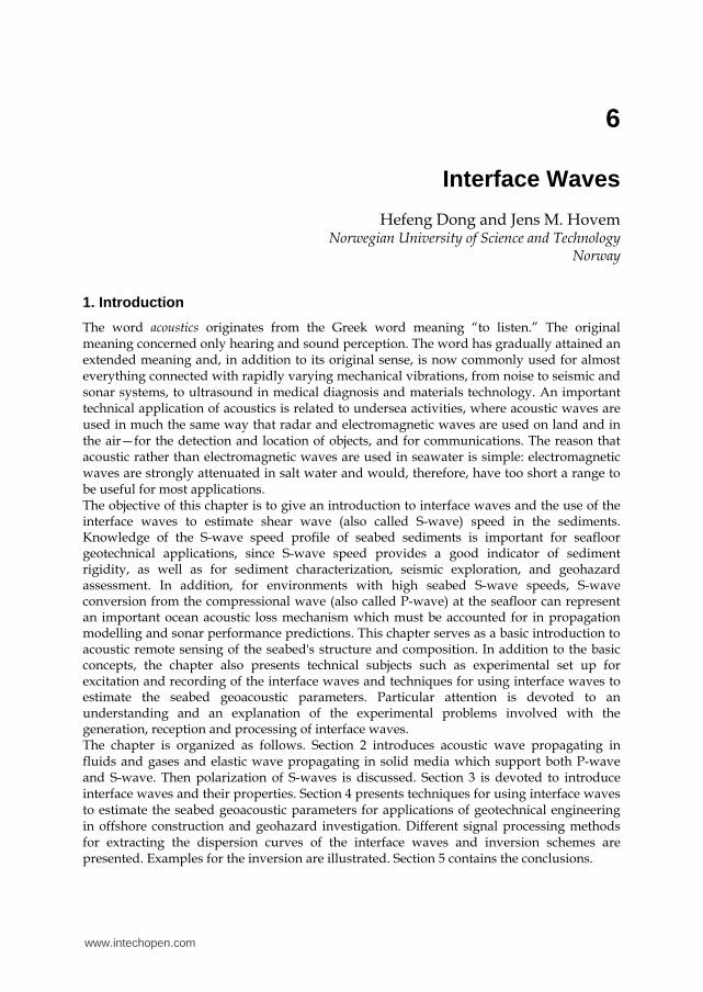
6

Interface Waves

Hefeng Dong and Jens M. Hovem Norwegian University of Science and Technology

Norway

1. Introduction

The word acoustics originates from the Greek word meaning “to listen.” The original meaning concerned only hearing and sound perception. The word has gradually attained an extended meaning and, in addition to its original sense, is now commonly used for almost everything connected with rapidly varying mechanical vibrations, from noise to seismic and sonar systems, to ultrasound in medical diagnosis and materials technology. An important technical application of acoustics is related to undersea activities, where acoustic waves are used in much the same way that radar and electromagnetic waves are used on land and in the air—for the detection and location of objects, and for communications. The reason that acoustic rather than electromagnetic waves are used in seawater is simple: electromagnetic waves are strongly attenuated in salt water and would, therefore, have too short a range to be useful for most applications. The objective of this chapter is to give an introduction to interface waves and the use of the interface waves to estimate shear wave (also called S-wave) speed in the sediments. Knowledge of the S-wave speed profile of seabed sediments is important for seafloor geotechnical applications, since S-wave speed provides a good indicator of sediment rigidity, as well as for sediment characterization, seismic exploration, and geohazard assessment. In addition, for environments with high seabed S-wave speeds, S-wave conversion from the compressional wave (also called P-wave) at the seafloor can represent an important ocean acoustic loss mechanism which must be accounted for in propagation modelling and sonar performance predictions. This chapter serves as a basic introduction to acoustic remote sensing of the seabed's structure and composition. In addition to the basic concepts, the chapter also presents technical subjects such as experimental set up for excitation and recording of the interface waves and techniques for using interface waves to estimate the seabed geoacoustic parameters. Particular attention is devoted to an understanding and an explanation of the experimental problems involved with the generation, reception and processing of interface waves. The chapter is organized as follows. Section 2 introduces acoustic wave propagating in fluids and gases and elastic wave propagating in solid media which support both P-wave and S-wave. Then polarization of S-waves is discussed. Section 3 is devoted to introduce interface waves and their properties. Section 4 presents techniques for using interface waves to estimate the seabed geoacoustic parameters for applications of geotechnical engineering in offshore construction and geohazard investigation. Different signal processing methods for extracting the dispersion curves of the interface waves and inversion schemes are presented. Examples for the inversion are illustrated. Section 5 contains the conclusions.

www.intechopen.com

Waves in Fluids and Solids 154

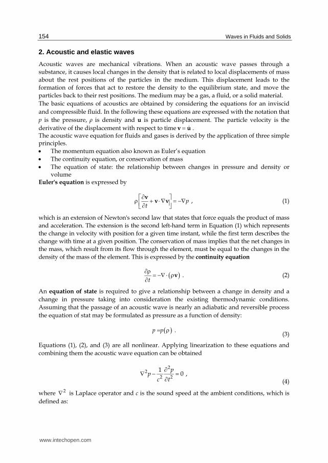
2. Acoustic and elastic waves

Acoustic waves are mechanical vibrations. When an acoustic wave passes through a substance, it causes local changes in the density that is related to local displacements of mass about the rest positions of the particles in the medium. This displacement leads to the formation of forces that act to restore the density to the equilibrium state, and move the particles back to their rest positions. The medium may be a gas, a fluid, or a solid material. The basic equations of acoustics are obtained by considering the equations for an inviscid and compressible fluid. In the following these equations are expressed with the notation that p is the pressure, ┩ is density and u is particle displacement. The particle velocity is the derivative of the displacement with respect to time v u . The acoustic wave equation for fluids and gases is derived by the application of three simple principles. The momentum equation also known as Euler’s equation The continuity equation, or conservation of mass The equation of state: the relationship between changes in pressure and density or

volume Euler's equation is expressed by

,pt

v

v v (1)

which is an extension of Newton's second law that states that force equals the product of mass and acceleration. The extension is the second left-hand term in Equation (1) which represents the change in velocity with position for a given time instant, while the first term describes the change with time at a given position. The conservation of mass implies that the net changes in the mass, which result from its flow through the element, must be equal to the changes in the density of the mass of the element. This is expressed by the continuity equation

.t

v (2)

An equation of state is required to give a relationship between a change in density and a change in pressure taking into consideration the existing thermodynamic conditions. Assuming that the passage of an acoustic wave is nearly an adiabatic and reversible process the equation of stat may be formulated as pressure as a function of density:

.p p (3)

Equations (1), (2), and (3) are all nonlinear. Applying linearization to these equations and combining them the acoustic wave equation can be obtained

22

2 21

0 ,p

pc t

(4)

where 2 is Laplace operator and c is the sound speed at the ambient conditions, which is defined as:

www.intechopen.com

Interface Waves 155

.K

c (5)

Thus the sound speed is given by the square root of the ratio between volume stiffness or bulk modulus K, which has the same dimension as pressure expressed in N/m2 or in pascal (Pa) and density, and the dimension of density is kg/m3. Both the volume stiffness and density are properties of the medium, and therefore depend on external conditions such as pressure and temperature. Therefore the sound speed is a local parameter, which may vary with the location, for instance, when the sound speed varies with the depth in the water. Equation (4) gives the wave equation for sound pressure. After linearization, the particle velocity is obtained from Newton’s second law

1

,pt

u

(6)

and the particle displacement satisfies the wave equation

2

2 21

0 .c t

u

u

(7)

It is often convenient to describe the particle displacement by a scalar variable as

, u (8)

is the displacement potential, which also satisfies the wave equation:

2

22 21

0 .c t

(9)

The sound pressure can be expressed by the displacement potential

2

2 .pt

(10)

By Fourier transformation, the wave equation is transformed from time domain to frequency domain:

( , ) ( , )exp( ) ,t i t dt

r r (11)

and back to time domain by the inverse transformation

1

( , ) ( , )exp( ) .2

t i t d

r r (12)

The wave equation for the displacement potential may be expressed in frequency domain as:

2 2( ) ( , ) 0 , r r (13)

www.intechopen.com

Waves in Fluids and Solids 156

where the wave number ( ) r is defined as

( ) .( )c

rr

(14)

Equation (13) is the Helmholtz equation, which is often easier to solve than the corresponding wave equation in time domain. A fluid medium can only support pressure or compressional waves also called P-waves or longitudinal waves with particle displacement in the direction of the wave propagation. A solid medium can in addition also support transverse waves or S-waves with particle displacement perpendicular to the direction of wave propagation. The wave equation in solid medium is given as:

2

22 ( 2 ) ( ) .

t

u

u u (15)

In this wave equation, ┣ and ┤ are Lamé elasticity coefficients, ┩ is the density of the medium, and u is the particle displacement vector with components ux, uy and uz. It is often convenient to recast equation (14) expressing the particle displacement vector by two potential functions, a scalar potential and a vector potential Ψ . The particle displacement vector is then expressed as:

. u Ψ (16)

Inserting equation (16) into equation (15) yields

2 2

2 2

2 + .

t t

Ψ Ψ

Ψ (17)

By definition, ( ) 0 Ψ . In equation (17), the terms containing and Ψ are independently selected to satisfy the respective parts of equation (17). This results in the following two wave equations:

2

22 2 ,

t

(18)

22

2 .t

Ψ Ψ

(19)

From Equation (18), we observe that the scalar potential propagates at a speed, called P-wave speed cp, defined as:

2

= .pH

c (20)

The vector potential Ψ of equation (19) propagates with the S-wave speed cs, defined as:

www.intechopen.com

Interface Waves 157

.sc (21)

The ratio between the two wave speeds defined by equations (20) and (21) is given by the Poisson ratio as:

1 2 .

2 1s

p

c

c

(22)

After inserting the two wave speeds into equations (18) and (19), respectively, the two wave equations are rewritten as

22

2 21

,pc t

(23)

2

22 21

.sc t

ΨΨ (24)

Equations (23) and (24) are the two wave equations relevant to acoustic-seismic wave propagation in an isotropic elastic medium. In a boundless, non-absorbing, homogeneous and isotropic solid these two types of body waves propagate independently of each other with speeds given by (20) and (21), respectively. In inhomogeneous media with space-dependent parameters, for instance at an interface between two different media, conversions between P-wave and S-wave take place, and vice versa. In many applications we are only interested in a two-dimensional case in which the particle movements are in the x-z plane and where there is no y-plane dependency. S-waves that are polarized so that the particle movement is in the x-z plane are called vertically polarized S-waves or SV waves. In general, S-waves are both vertically and horizontally polarized. The horizontal polarized S-waves are also called SH waves. However, in most underwater acoustic applications, we only need to consider vertically polarized S-waves since these are the waves that may be excited in the bottom by a normal volume source in the water column. An incident P-wave in a fluid medium at an interface between the fluid and a solid medium generates a reflected P-wave in the fluid and two transmitted waves: one P-wave and one S-wave. An incident P-wave at an interface between two solid media generates reflected P-wave and S-wave in the incident medium and transmitted P-wave and S-wave in the second medium. In any case the reflected and transmitted waves are determined by the boundary conditions, which require that the normal stress, normal particle displacement, tangential stress, and tangential particle displacement are continuous at the interface. In the fluid, the tangential stress is zero and there is no constraint on the tangential particle displacement.

3. Interface waves

In this section we introduce interface waves and their properties (Rauch, 1980). The simplest type of interface wave is the well-known Rayleigh wave, which can propagate along a free

www.intechopen.com

Waves in Fluids and Solids 158

surface of a solid medium and has a penetration depth of about one wavelength of the Rayleigh wave. A Scholte wave is another wave of the same type that can propagate at a fluid/solid interface and its decay inside the solid is comparable with that of the Rayleigh wave. The penetration depth in the fluid remains small when the adjacent solid is very soft, that is when the S-wave speed in the solid is smaller than the sound speed in the fluid. This is the situation for most water/unconsolidated-sediment combinations. But the penetration depth can be much larger if the S-wave speed in the solid is larger than the sound speed in the fluid, as is normally the case for all water/rock combinations. The most complicated type of interface wave is the well-known Stoneley wave, which can occur at the interface between two solid media for only limited combinations of parameters. Its penetration depth into each of the solid media is similar to that of the Rayleigh wave. The existence of the interface waves discussed above requires that at least one of the two media is a solid while the other medium may be a vacuum, air, a fluid or a solid. Love wave is another type of interface wave which is related to SH wave polarized parallel to a given interface and propagates within solid layers. It is guided by a free surface or a fluid/solid interface (Love, 1926; Sato, 1954).

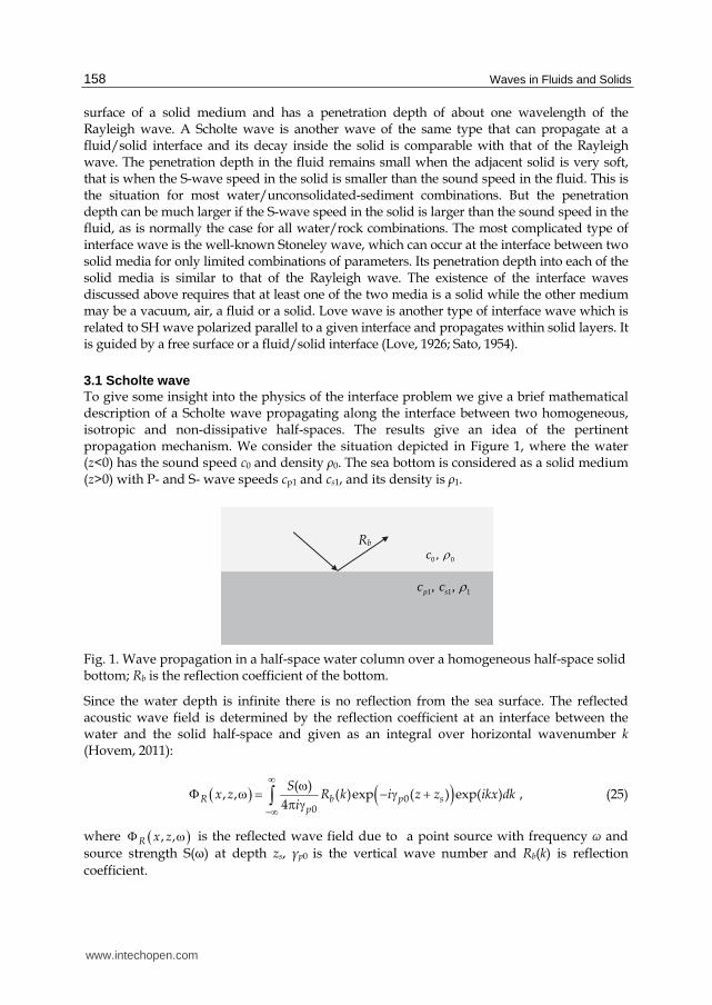
3.1 Scholte wave To give some insight into the physics of the interface problem we give a brief mathematical description of a Scholte wave propagating along the interface between two homogeneous, isotropic and non-dissipative half-spaces. The results give an idea of the pertinent propagation mechanism. We consider the situation depicted in Figure 1, where the water (z<0) has the sound speed c0 and density ┩0. The sea bottom is considered as a solid medium (z>0) with P- and S- wave speeds cp1 and cs1, and its density is ┩1.

Fig. 1. Wave propagation in a half-space water column over a homogeneous half-space solid bottom; Rb is the reflection coefficient of the bottom.

Since the water depth is infinite there is no reflection from the sea surface. The reflected acoustic wave field is determined by the reflection coefficient at an interface between the water and the solid half-space and given as an integral over horizontal wavenumber k (Hovem, 2011):

00

( ), , ( )exp ( ) exp( ) ,

4R b p sp

Sx z R k i z z ikx dk

i

(25)

where , ,R x z is the reflected wave field due to a point source with frequency ω and source strength S(┱) at depth zs, γp0 is the vertical wave number and Rb(k) is reflection coefficient.

0 0, c 1 1 1, , p sc c

Rb

www.intechopen.com

Interface Waves 159

Consider a plane, monochromatic wave of angular frequency ┱ = 2┨f propagating in the +x direction – the problem becomes two-dimensional (no y-coordinate dependency). Therefore the particle displacement has only two components u = (ux, uz) and the vector potential has only one component ψ = (0, ┰, 0). The two components of the particle displacement in equation (16) are then defined as:

,

.

x

z

ux z

uz x

(26a)

(26b)

The components of the stress expressed by the potentials are

2 20 0

0 0 0 2 2

0 0

xx zz

xz

px z

,

(27a)

(27b)

in the water, and

2 2 2 21 1 1 1

1 1 1 12 2 2

2 2 21 1 1

1 1 2 2

2 2 2 21 1 1 1

1 1 1 12 2 2

2 2

2

2 2

xx

xz

zz

x zx z z

x z x z

x zx z x

,

(28a)

(28b)

(28c)

in the bottom. The boundary conditions at the interface between the water and the solid bottom at z = 0 are

0 1

1

1 0

z z

zz

xz

u u

p

.

(29a)

(29b)

(29c)

Assuming the displacement potentials of the form:

0 0exp exp (z 0) ,pA z i kx t (30)

1 1

1 1

exp exp (z 0)

exp exp (z 0)

p

s

B z i kx t

C z i kx t

.(31a)

(31b)

The potentials have to fulfil the wave equations:

www.intechopen.com

Waves in Fluids and Solids 160

2 2

0 0 0 0 . (32)

in the water, and

2 2

1 1 1 0 ,p (33)

2 2

1 1 1 0 ,s (34)

in the solid bottom. Since the horizontal wave number, k, is the same for all waves at the interface, the vertical wave numbers describing the vertical decays of the fields have to be

2 20 0 0

2 21 1 1

2 21 1 1

p p p

p p p

s s s

i k

i k

i k

,

(35a)

(35b)

(35c)

where

0 1 10 1 1

, , , .p p sp p p s

kv c c c

(36)

are the horizontal wave number, the wave numbers for the P-wave in the water and the P- and S-waves in the bottom, respectively, and vp is the phase speed. The use of the boundary conditions Equation (29) leads to a set of three equations for the amplitudes A, B, and C.

2 21 1

2 2 2 20 0 1 1 1 1 1 1

0 1

0 2 ( ) 0( ) ( 2 ) 2 = 0 .

0

p s

p p s

p p

ik k A

Bk k i k

Cik

(37)

The relationship between these amplitudes are given by 2 2

1 02

11

021

2

s p

ps

p

s

kB A

ikC A

.

(38a)

(38b)

The set of homogeneous, linear equations (37) has a non-trivial solution only if the coefficient determinant is vanishing, which results in:

2 42

1 1 102 2 2

1 1 014 2 .p s p

s ps kck k c

(39)

www.intechopen.com

Interface Waves 161

Inserting equations (35) and (36) into equation (39), we get the expression for the phase speed of the Scholte wave

2

22 2 4210

2 21 1 1 11

0

1

4 1 1 2 .

1

p

pp p p p

p s ssp

p

v

cv v v v

c c cc v

c

(40)

Equation (40) has always one positive real root, which is the Scholte wave p Schv v and can be found numerically. In the general situation with finite water depth, D, the sound propagates as in a waveguide by reflections from both the sea surface and the bottom. The sound field in a waveguide is given by an integral over horizontal wave numbers (Equation (17.66) in Hovem, 2011). The solution of this integral is approximately found by using the residue technique as the sum of the residues at the poles of the integrand. The poles are given by the zeros of the denominator of the integrand

01 exp( 2 ) 0 ,b s pR R D (41)

where Rs and Rb are reflection coefficients of the sea surface and the bottom, respectively. Assume that at the sea surface Rs= -1 and the poles are given as the solution to

01 exp( 2 ) 0 .b pR D (42)

Using the expression of the reflection coefficient of the bottom (Equation (15.42) in Hovem, 2011) we can get

2 421 1 10

02 2 21 0 11

4 2 tanh .p s pp

p ss

Dkck k c

(43)

By applying equations (35) and (36), this expression can be transformed into

22 2 2

21 1 1

2

2410

21 1 0

0

4 1 1 2

1

tanh 1 .

1

p p p

p s s

p

pp p

s p pp

p

v v v

c c c

v

cv vD

c v cv

c

(44)

Equation (44) is the dispersion equation for the case with finite water depth and we see that, when D→∞, this expression becomes identical to the expression of equation (40) for the

www.intechopen.com

Waves in Fluids and Solids 162

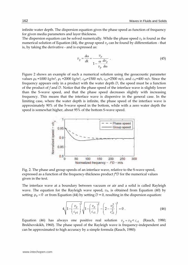
infinite water depth. The dispersion equation gives the phase speed as function of frequency for given media parameters and layer thickness. The dispersion equation can be solved numerically. While the phase speed vp is found as the numerical solution of Equation (44), the group speed vg can be found by differentiation - that is, by taking the derivative - and is expressed as:

.1

pg

p

p

vdv

dvdk

v d

(45)

Figure 2 shows an example of such a numerical solution using the geoacoustic parameter values ρ0 =1000 kg/m3, ρ1 =2000 kg/m3, cp0=1500 m/s, cp1=2500 m/s, and cs1=400 m/s. Since the frequency appears only in a product with the water depth D, the speed must be a function of the product of f and D. Notice that the phase speed of the interface wave is slightly lower than the S-wave speed, and that the phase speed decreases slightly with increasing frequency. This means that the interface wave is dispersive in the general case. In the limiting case, where the water depth is infinite, the phase speed of the interface wave is approximately 90% of the S-wave speed in the bottom, while with a zero water depth the speed is somewhat higher, about 95% of the bottom S-wave speed.

Fig. 2. The phase and group speeds of an interface wave, relative to the S-wave speed, expressed as a function of the frequency-thickness product f*D for the numerical values given in the text.

The interface wave at a boundary between vacuum or air and a solid is called Rayleigh wave. The equation for the Rayleigh wave speed, vR, is obtained from Equation (40) by setting 0 0 or from Equation (44) by setting D = 0, resulting in the dispersion equation:

22 2 2

21 1 1

4 1 1 2 0 .p p p

p s s

v v v

c c c

(46)

Equation (46) has always one positive real solution 1< p R sv v c (Rauch, 1980; Brekhovskikh, 1960). The phase speed of the Rayleigh wave is frequency-independent and can be approximated to high accuracy by a simple formula (Rauch, 1980):

www.intechopen.com

Interface Waves 163

10.87 1.12

.1R sv c (47)

where ┥ is the Poisson’s ratio. The phase speed of the Rayleigh is approximately 95% of the S-wave speed, as can be seen in Figure 2. Thus, in a solid medium a measurement of the Rayleigh wave speed may also give an accurate measure of S-wave speed. The phase speed vp of the Scholte wave is also frequency-independent, and always slightly smaller than the lowest speed occurring in any of the two bordering media i.e. vp < min (cp0, cs1). With the use of hydrophones in the water or geophones on or in the bottom, one can detect and record the sound pressure within the water mass and the components of the particle displacement in the solid bottom. We will now determine the real components of the displacement vector of the Scholte wave. Using equations (26), (30), (31) and (36), the displacement components are expressed as 0 0

0 0

ˆ ( , )sin , ( 0)ˆ ( , )cos , ( 0)

x x

z z

u u k z kx t z

u u k z kx t z

,

(48a)

(48b)

where 0 0

0 0 0

ˆ ( , ) exp

ˆ ( , ) exp

x p

z p p

u k z kA z

u k z A z

,

(49a)

(49b)

in the water, and 1 1

1 1

ˆ ( , )sin , ( 0)ˆ ( , )cos , ( 0)

x x

z z

u u k z kx t z

u u k z kx t z

, (50a)

(50b)

where

0 2 21 1 1 1 1 12

1 1

0 2 2 21 1 1 12

1

ˆ 2 exp ( )exp

ˆ 2 exp ( )exp

( , )

( , )

p

x p s s s p

s p

p

z s s p

s

u z k z

u k z k z

kAk z

Ak z

,

(51a)

(51b)

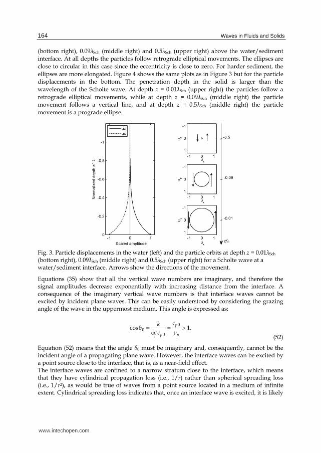
in the bottom. Equations (48) - (51) are parametric representations of ellipses having their main axes parallel to the axes of the coordinate system. With increasing distance from the interface, the displacement amplitudes 0 0ˆ ˆ, x zu u and 1ˆzu decrease exponentially without changing sign. The horizontal displacement in the bottom, 1ˆxu , shows the same asymptotic behaviour, but with the sign changing at the depth of about one-tenth of the Scholte wavelength. Figure 3 plots the particle displacements as a function of depth relative to the Scholte wavelength ┣Sch in the water column (left panel) and the particle orbits (right panels) for a typical water/sediment interface. The same parameters are used as in Figure 2 and the frequency-thickness product f*D = 200. The penetration depth in the water is about one-half of the Scholte wavelength. The right panels plot the particle movement at depth z = 0.01┣Sch

www.intechopen.com

Waves in Fluids and Solids 164

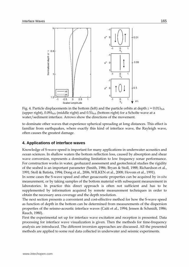
(bottom right), 0.09┣Sch (middle right) and 0.5┣Sch (upper right) above the water/sediment interface. At all depths the particles follow retrograde elliptical movements. The ellipses are close to circular in this case since the eccentricity is close to zero. For harder sediment, the ellipses are more elongated. Figure 4 shows the same plots as in Figure 3 but for the particle displacements in the bottom. The penetration depth in the solid is larger than the wavelength of the Scholte wave. At depth z = 0.01┣Sch (upper right) the particles follow a retrograde elliptical movements, while at depth z = 0.09┣Sch (middle right) the particle movement follows a vertical line, and at depth z = 0.5┣Sch (middle right) the particle movement is a prograde ellipse.

Fig. 3. Particle displacements in the water (left) and the particle orbits at depth z = 0.01┣Sch (bottom right), 0.09┣Sch (middle right) and 0.5┣Sch (upper right) for a Scholte wave at a water/sediment interface. Arrows show the directions of the movement.

Equations (35) show that all the vertical wave numbers are imaginary, and therefore the signal amplitudes decrease exponentially with increasing distance from the interface. A consequence of the imaginary vertical wave numbers is that interface waves cannot be excited by incident plane waves. This can be easily understood by considering the grazing angle of the wave in the uppermost medium. This angle is expressed as:

00

0cos 1.p

p p

ck

c v

(52)

Equation (52) means that the angle θ0 must be imaginary and, consequently, cannot be the incident angle of a propagating plane wave. However, the interface waves can be excited by a point source close to the interface, that is, as a near-field effect. The interface waves are confined to a narrow stratum close to the interface, which means that they have cylindrical propagation loss (i.e., 1/r) rather than spherical spreading loss (i.e., 1/r2), as would be true of waves from a point source located in a medium of infinite extent. Cylindrical spreading loss indicates that, once an interface wave is excited, it is likely

www.intechopen.com

Interface Waves 165

Fig. 4. Particle displacements in the bottom (left) and the particle orbits at depth z = 0.01┣Sch (upper right), 0.09┣Sch (middle right) and 0.5┣Sch (bottom right) for a Scholte wave at a water/sediment interface. Arrows show the directions of the movement.

to dominate other waves that experience spherical spreading at long distances. This effect is familiar from earthquakes, where exactly this kind of interface wave, the Rayleigh wave, often causes the greatest damage.

4. Applications of interface waves

Knowledge of S-wave speed is important for many applications in underwater acoustics and ocean sciences. In shallow waters the bottom reflection loss, caused by absorption and shear wave conversion, represents a dominating limitation to low frequency sonar performance. For construction works in water, geohazard assessment and geotechnical studies the rigidity of the seabed is an important parameter (Smith, 1986; Bryan & Stoll, 1988; Richardson et al., 1991; Stoll & Batista, 1994; Dong et al., 2006, WILKEN et al., 2008; Hovem et al., 1991). In some cases the S-wave speed and other geoacoustic properties can be acquired by in-situ measurement, or by taking samples of the bottom material with subsequent measurement in laboratories. In practice this direct approach is often not sufficient and has to be supplemented by information acquired by remote measurement techniques in order to obtain the necessary area coverage and the depth resolution. The next section presents a convenient and cost-effective method for how the S-wave speed as function of depth in the bottom can be determined from measurements of the dispersion properties of the seismo-acoustic interface waves (Caiti et al., 1994; Jensen & Schmidt, 1986; Rauch, 1980). First the experimental set up for interface wave excitation and reception is presented. Data processing for interface wave visualization is given. Then the methods for time-frequency analysis are introduced. The different inversion approaches are discussed. All the presented methods are applied to some real data collected in underwater and seismic experiments.

www.intechopen.com

Waves in Fluids and Solids 166

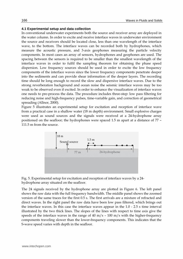
4.1 Experimental setup and data collection In conventional underwater experiments both the source and receiver array are deployed in the water column. In order to excite and receive interface waves in underwater environment the source and receivers should be located close, less than one wavelength of the interface wave, to the bottom. The interface waves can be recorded both by hydrophones, which measure the acoustic pressure, and 3-axis geophones measuring the particle velocity components. In most cases an array of sensors, hydrophones and geophones are used. The spacing between the sensors is required to be smaller than the smallest wavelength of the interface waves in order to fulfil the sampling theorem for obtaining the phase speed dispersion. Low frequency sources should be used in order to excite the low frequency components of the interface waves since the lower frequency components penetrate deeper into the sediments and can provide shear information of the deeper layers. The recording time should be long enough to record the slow and dispersive interface waves. Due to the strong reverberation background and ocean noise the seismic interface waves may be too weak to be observed even if excited. In order to enhance the visualization of interface waves one needs to pre-process the data. The procedure includes three-step: low pass filtering for reducing noise and high-frequency pulses, time-variable gain, and correction of geometrical spreading (Allnor, 2000). Figure 5 illustrates an experimental setup for excitation and reception of interface wave from a practical case in a shallow water (18 m depth) environment. Small explosive charges were used as sound sources and the signals were received at a 24-hydrophone array positioned on the seafloor; the hydrophones were spaced 1.5 m apart at a distance of 77 – 111.5 m from the source.

Fig. 5. Experimental setup for excitation and reception of interface waves by a 24-hydrophone array situated on the seafloor.

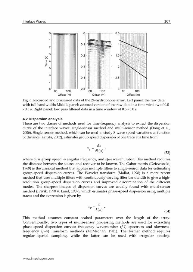
The 24 signals received by the hydrophone array are plotted in Figure 6. The left panel shows the raw data with the full frequency bandwidth. The middle panel shows the zoomed version of the same traces for the first 0.5 s. The first arrivals are a mixture of refracted and direct waves. In the right panel the raw data have been low pass filtered, which brings out the interface waves. In this case the interface waves appear in the 1.0 - 2.5 s time interval illustrated by the two thick lines. The slopes of the lines with respect to time axis give the speeds of the interface waves in the range of 40 m/s – 100 m/s with the higher-frequency components traveling slower than the lower-frequency components. This indicates that the S-wave speed varies with depth in the seafloor.

77 m 24-hydrophone

Sound source 1.5 m

18 m

www.intechopen.com

Interface Waves 167

Fig. 6. Recorded and processed data of the 24-hydrophone array. Left panel: the raw data with full bandwidth; Middle panel: zoomed version of the raw data in a time window of 0.0 - 0.5 s. Right panel: low pass filtered data in a time window of 0.5 - 3.0 s.

4.2 Dispersion analysis There are two classes of methods used for time-frequency analysis to extract the dispersion curve of the interface waves: single-sensor method and multi-sensor method (Dong et al., 2006). Single-sensor method, which can be used to study S-wave speed variations as function of distance (Kritski, 2002), estimates group speed dispersion of one trace at a time from

,

( )gd

vdk

(53)

where vg is group speed, ω angular frequency, and k(ω) wavenumber. This method requires the distance between the source and receiver to be known. The Gabor matrix (Dziewonski, 1969) is the classical method that applies multiple filters to single-sensor data for estimating group-speed dispersion curves. The Wavelet transform (Mallat, 1998) is a more recent method that uses multiple filters with continuously varying filter bandwidth to give a high-resolution group-speed dispersion curves and improved discrimination of the different modes. The sharpest images of dispersion curves are usually found with multi-sensor method (Frivik, 1998 & Land, 1987), which estimates phase-speed dispersion using multiple traces and the expression is given by

.

( )pvk

(54)

This method assumes constant seabed parameters over the length of the array. Conventionally, two types of multi-sensor processing methods are used for extracting phase-speed dispersion curves: frequency wavenumber (f-k) spectrum and slowness-frequency (p-ω) transform methods (McMechan, 1981). The former method requires regular spatial sampling, while the latter can be used with irregular spacing.

www.intechopen.com

Waves in Fluids and Solids 168

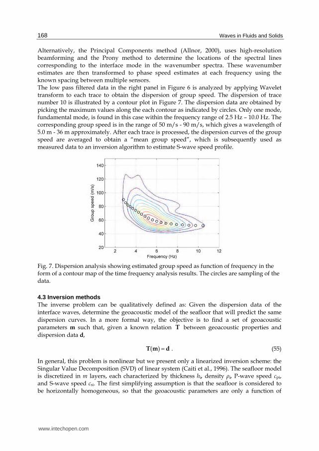
Alternatively, the Principal Components method (Allnor, 2000), uses high-resolution beamforming and the Prony method to determine the locations of the spectral lines corresponding to the interface mode in the wavenumber spectra. These wavenumber estimates are then transformed to phase speed estimates at each frequency using the known spacing between multiple sensors. The low pass filtered data in the right panel in Figure 6 is analyzed by applying Wavelet transform to each trace to obtain the dispersion of group speed. The dispersion of trace number 10 is illustrated by a contour plot in Figure 7. The dispersion data are obtained by picking the maximum values along the each contour as indicated by circles. Only one mode, fundamental mode, is found in this case within the frequency range of 2.5 Hz – 10.0 Hz. The corresponding group speed is in the range of 50 m/s - 90 m/s, which gives a wavelength of 5.0 m - 36 m approximately. After each trace is processed, the dispersion curves of the group speed are averaged to obtain a “mean group speed”, which is subsequently used as measured data to an inversion algorithm to estimate S-wave speed profile.

Fig. 7. Dispersion analysis showing estimated group speed as function of frequency in the form of a contour map of the time frequency analysis results. The circles are sampling of the data.

4.3 Inversion methods The inverse problem can be qualitatively defined as: Given the dispersion data of the interface waves, determine the geoacoustic model of the seafloor that will predict the same dispersion curves. In a more formal way, the objective is to find a set of geoacoustic parameters m such that, given a known relation T between geoacoustic properties and dispersion data d,

( ) .┌ m d (55)

In general, this problem is nonlinear but we present only a linearized inversion scheme: the Singular Value Decomposition (SVD) of linear system (Caiti et al., 1996). The seafloor model is discretized in m layers, each characterized by thickness hi, density ┩i, P-wave speed cpi, and S-wave speed csi. The first simplifying assumption is that the seafloor is considered to be horizontally homogeneous, so that the geoacoustic parameters are only a function of

www.intechopen.com

Interface Waves 169

depth in the sediment. The second simplifying assumption is that the dispersion of the interface wave at the water-sediment interface is only a function of S-wave speed of the bottom materials and the layering. The other geoacoustic properties are fixed and not changed during the inversion procedure since the dispersion is not sensitive to these parameters. These assumptions reduce the number of parameters to be estimated and the computational effort needed, but do not seriously affect the accuracy of the estimates. The actual computation of the predicted dispersion of phase/group speed is performed with a standard Thomson-Haskell integration scheme (Haskell, 1953), which has the advantage of being fast and economical in terms of computer usage. However, different codes can be used to generate predictions without affecting the structure of the inversion algorithm. With the assumptions the model generates the dispersion of phase/group speed

np v R as function of the S-wave speed m

s c R :

,s pTc v (56)

where Jacobian n m ┌ R R . Depending on the system represented by equation (55) is over- or underdetermined, its solution may not exist or may not be unique. So it is customary to look for a solution of (56) in the least square sense; that is, a vector cs that minimizes

2s pTc v . Consider the most common case where m < n; that is, we have more data than

parameters to be estimated. The least-square solution is found by solving the normal equation:

1( ) .T T

s pc T T T v

(57)

Here TT is the transpose conjugate of matrix T. By using the SVD to the rectangular matrix T the solution can be expressed as:

,T

s p -1c W┋ U v (58)

1 1

( ).

Tm mi p i

s i ii ii i

u vc w w (59)

In equations (57), (58) and (59) [ ]T TT W ┋ O U , U and W are unitary orthogonal matrices with dimension (nn) and (mm) respectively and ┋ is a square diagonal matrix of dimension m, with diagonal entries i called singular values of T with 12…m; O is a zero matrix with dimension (m(n-m)); ui is the ith column of U and wj the jth column of W. Since the matrix ┋ is ill conditioned in the numerical solution of this inverse problem a technique called regularization is used to deal with the ill conditioning (Tikhonov & Arsenin, 1977). The regularized solution is given by:

.T T Ts p -1c (T T + H H) T v (60)

H with dimension (mm) is a generic operator that embeds the a priori constraints imposed on the solution and regularization parameter ┣ > 0. The detailed discussion on regularization can be found in (Caiti et al., 1994). The regularized solution is given by

www.intechopen.com

Waves in Fluids and Solids 170

† ,s pTc v (61)

with

.T T† -1 -1T = W(┋+┋ (HW) (HW)) U (62)

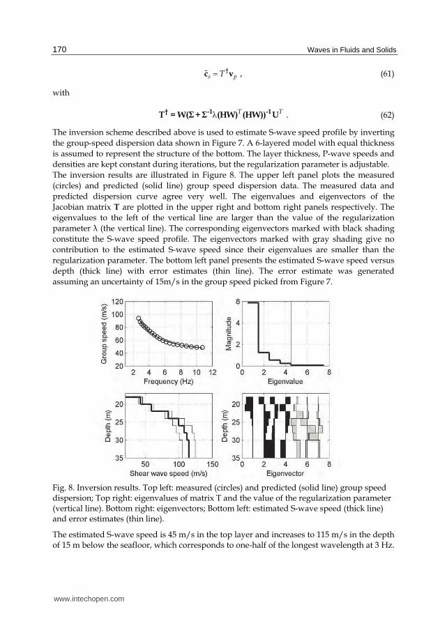
The inversion scheme described above is used to estimate S-wave speed profile by inverting the group-speed dispersion data shown in Figure 7. A 6-layered model with equal thickness is assumed to represent the structure of the bottom. The layer thickness, P-wave speeds and densities are kept constant during iterations, but the regularization parameter is adjustable. The inversion results are illustrated in Figure 8. The upper left panel plots the measured (circles) and predicted (solid line) group speed dispersion data. The measured data and predicted dispersion curve agree very well. The eigenvalues and eigenvectors of the Jacobian matrix T are plotted in the upper right and bottom right panels respectively. The eigenvalues to the left of the vertical line are larger than the value of the regularization parameter ┣ (the vertical line). The corresponding eigenvectors marked with black shading constitute the S-wave speed profile. The eigenvectors marked with gray shading give no contribution to the estimated S-wave speed since their eigenvalues are smaller than the regularization parameter. The bottom left panel presents the estimated S-wave speed versus depth (thick line) with error estimates (thin line). The error estimate was generated assuming an uncertainty of 15m/s in the group speed picked from Figure 7.

Fig. 8. Inversion results. Top left: measured (circles) and predicted (solid line) group speed dispersion; Top right: eigenvalues of matrix T and the value of the regularization parameter (vertical line). Bottom right: eigenvectors; Bottom left: estimated S-wave speed (thick line) and error estimates (thin line).

The estimated S-wave speed is 45 m/s in the top layer and increases to 115 m/s in the depth of 15 m below the seafloor, which corresponds to one-half of the longest wavelength at 3 Hz.

www.intechopen.com

Interface Waves 171

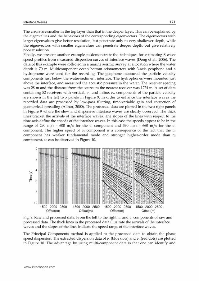
The errors are smaller in the top layer than that in the deeper layer. This can be explained by the eigenvalues and the behaviors of the corresponding eigenvectors. The eigenvectors with larger eigenvalues give better resolution, but penetrate only to very shallower depth, while the eigenvectors with smaller eigenvalues can penetrate deeper depth, but give relatively poor resolution. Finally, we present another example to demonstrate the techniques for estimating S-wave speed profiles from measured dispersion curves of interface waves (Dong et al., 2006). The data of this example were collected in a marine seismic survey at a location where the water depth is 70 m. Multicomponent ocean bottom seismometers with 3-axis geophone and a hydrophone were used for the recording. The geophone measured the particle velocity components just below the water-sediment interface. The hydrophones were mounted just above the interface, and measured the acoustic pressure in the water. The receiver spacing was 28 m and the distance from the source to the nearest receiver was 1274 m. A set of data containing 52 receivers with vertical, vz, and inline, vx, components of the particle velocity are shown in the left two panels in Figure 9. In order to enhance the interface waves the recorded data are processed by low-pass filtering, time-variable gain and correction of geometrical spreading (Allnor, 2000). The processed data are plotted in the two right panels in Figure 9 where the slow and dispersive interface waves are clearly observed. The thick lines bracket the arrivals of the interface waves. The slopes of the lines with respect to the time-axis define the speeds of the interface waves. In this case the speeds appear to be in the range of 290 m/s - 600 m/s for the vz component and 390 m/s - 660 m/s for the vx component. The higher speed of vx component is a consequence of the fact that the vx component has weaker fundamental mode and stronger higher-order mode than vz component, as can be observed in Figure 10.

Fig. 9. Raw and processed data. From the left to the right: vz and vx components of raw and processed data. The thick lines in the processed data illustrate the arrivals of the interface waves and the slopes of the lines indicate the speed range of the interface waves.

The Principal Components method is applied to the processed data to obtain the phase speed dispersion. The extracted dispersion data of vz (blue dots) and vx (red dots) are plotted in Figure 10. The advantage by using multi-component data is that one can identify and

www.intechopen.com

Waves in Fluids and Solids 172

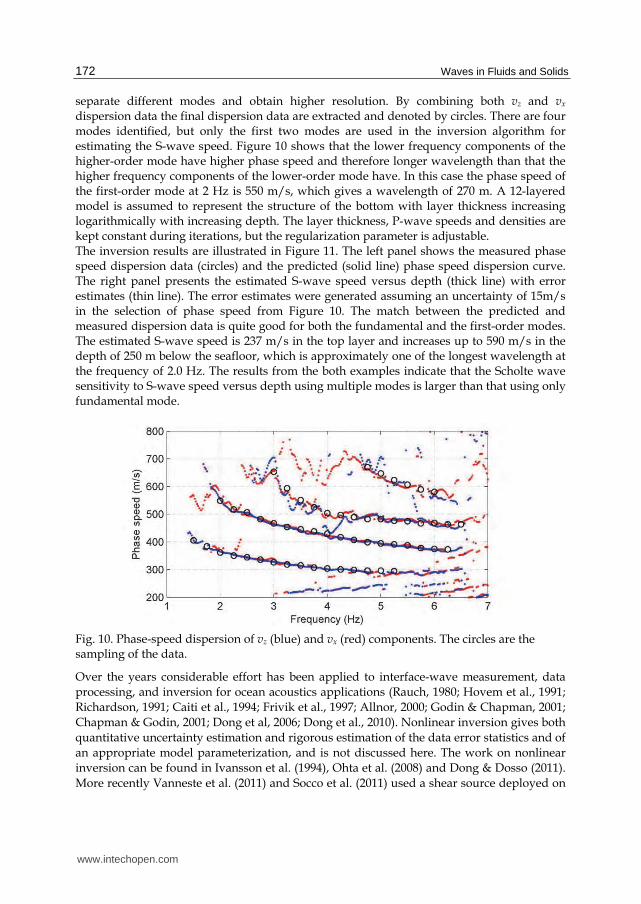
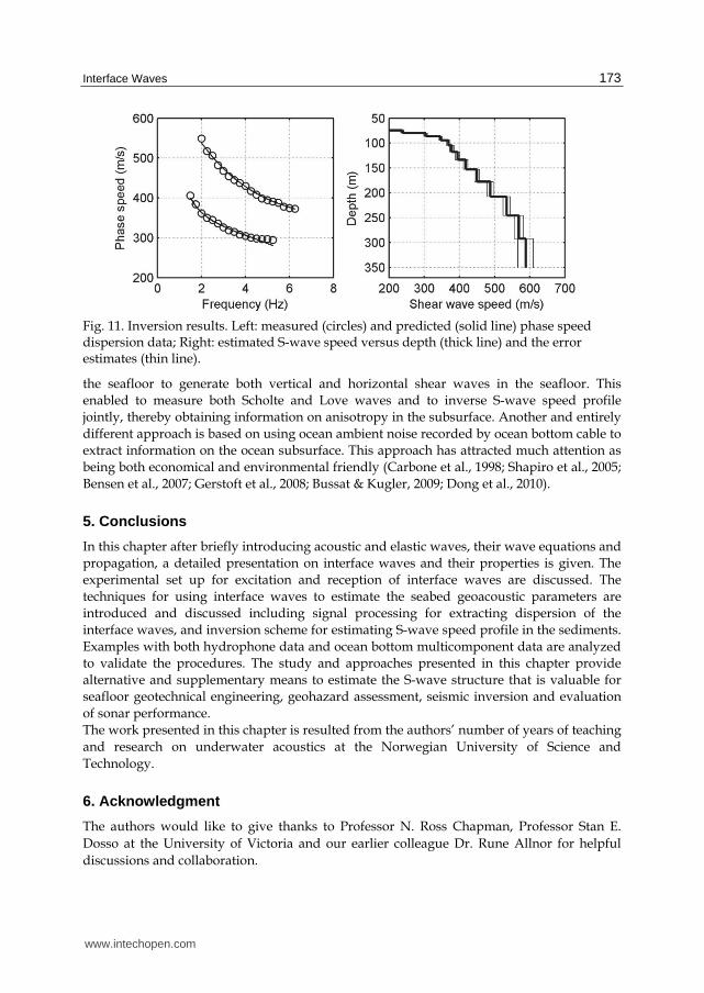
separate different modes and obtain higher resolution. By combining both vz and vx dispersion data the final dispersion data are extracted and denoted by circles. There are four modes identified, but only the first two modes are used in the inversion algorithm for estimating the S-wave speed. Figure 10 shows that the lower frequency components of the higher-order mode have higher phase speed and therefore longer wavelength than that the higher frequency components of the lower-order mode have. In this case the phase speed of the first-order mode at 2 Hz is 550 m/s, which gives a wavelength of 270 m. A 12-layered model is assumed to represent the structure of the bottom with layer thickness increasing logarithmically with increasing depth. The layer thickness, P-wave speeds and densities are kept constant during iterations, but the regularization parameter is adjustable. The inversion results are illustrated in Figure 11. The left panel shows the measured phase speed dispersion data (circles) and the predicted (solid line) phase speed dispersion curve. The right panel presents the estimated S-wave speed versus depth (thick line) with error estimates (thin line). The error estimates were generated assuming an uncertainty of 15m/s in the selection of phase speed from Figure 10. The match between the predicted and measured dispersion data is quite good for both the fundamental and the first-order modes. The estimated S-wave speed is 237 m/s in the top layer and increases up to 590 m/s in the depth of 250 m below the seafloor, which is approximately one of the longest wavelength at the frequency of 2.0 Hz. The results from the both examples indicate that the Scholte wave sensitivity to S-wave speed versus depth using multiple modes is larger than that using only fundamental mode.

Fig. 10. Phase-speed dispersion of vz (blue) and vx (red) components. The circles are the sampling of the data.

Over the years considerable effort has been applied to interface-wave measurement, data processing, and inversion for ocean acoustics applications (Rauch, 1980; Hovem et al., 1991; Richardson, 1991; Caiti et al., 1994; Frivik et al., 1997; Allnor, 2000; Godin & Chapman, 2001; Chapman & Godin, 2001; Dong et al, 2006; Dong et al., 2010). Nonlinear inversion gives both quantitative uncertainty estimation and rigorous estimation of the data error statistics and of an appropriate model parameterization, and is not discussed here. The work on nonlinear inversion can be found in Ivansson et al. (1994), Ohta et al. (2008) and Dong & Dosso (2011). More recently Vanneste et al. (2011) and Socco et al. (2011) used a shear source deployed on

www.intechopen.com

Interface Waves 173

Fig. 11. Inversion results. Left: measured (circles) and predicted (solid line) phase speed dispersion data; Right: estimated S-wave speed versus depth (thick line) and the error estimates (thin line).

the seafloor to generate both vertical and horizontal shear waves in the seafloor. This enabled to measure both Scholte and Love waves and to inverse S-wave speed profile jointly, thereby obtaining information on anisotropy in the subsurface. Another and entirely different approach is based on using ocean ambient noise recorded by ocean bottom cable to extract information on the ocean subsurface. This approach has attracted much attention as being both economical and environmental friendly (Carbone et al., 1998; Shapiro et al., 2005; Bensen et al., 2007; Gerstoft et al., 2008; Bussat & Kugler, 2009; Dong et al., 2010).

5. Conclusions

In this chapter after briefly introducing acoustic and elastic waves, their wave equations and propagation, a detailed presentation on interface waves and their properties is given. The experimental set up for excitation and reception of interface waves are discussed. The techniques for using interface waves to estimate the seabed geoacoustic parameters are introduced and discussed including signal processing for extracting dispersion of the interface waves, and inversion scheme for estimating S-wave speed profile in the sediments. Examples with both hydrophone data and ocean bottom multicomponent data are analyzed to validate the procedures. The study and approaches presented in this chapter provide alternative and supplementary means to estimate the S-wave structure that is valuable for seafloor geotechnical engineering, geohazard assessment, seismic inversion and evaluation of sonar performance. The work presented in this chapter is resulted from the authors’ number of years of teaching and research on underwater acoustics at the Norwegian University of Science and Technology.

6. Acknowledgment

The authors would like to give thanks to Professor N. Ross Chapman, Professor Stan E. Dosso at the University of Victoria and our earlier colleague Dr. Rune Allnor for helpful discussions and collaboration.

www.intechopen.com

Waves in Fluids and Solids 174

7. References

Allnor, R. (2000). Seismo-Acoustic Remote Sensing of Shear Wave Velocities in Shallow Marine Sediments, PhD. Thesis, No. 420006, Norwegian University of Science and Technology, Trondheim, Norway

Brekhovskikh, L. M. (1960). Waves in Layered media, Academic Press, New York, N. Y. USA Bryan, G. M. & Stoll, R. D. (1988). The Dynamic Shear Modulus of Marine Sediments, J.

Acoust. Soc. Am., Vol. 83, pp. 2159-2164 Bucker, H. P. (1970). Sound Propagation in a Channel with Lossy Boundaries, J. Acoust. Soc.

Am. Vol. 48, pp. 1187-1194 Bussat, S. & Kugler, S. (2009). Recording Noise - Estimating Shear-Wave Velocities:

Feasibility of Offshore Ambient- Noise Surface Wave Tomography (ANSWT) on a Reservior Scale, SEG Expanded Abstracts, pp. 1627-1631

Caiti, A., Akal, T. & Stoll, R.D. (1994). Estimation of Shear Wave Velocity in Shallow Marine Sediments, IEEE J. Ocean. Eng., Vol. 19, pp. 58-72

Carbone, N. M., Deane, G. B. & Buckingham, M. J. (1998). Estimating the compressional and shear wave speeds of a shallow water seabed from the vertical coherence of ambient noise in the water column, J. Acoust. Soc. Am., Vol. 103(2), pp. 801-813

Chapman, D. M. F. & Godin, O. A. (2001). Dispersion of Interface Waves in Sediments with Power-Law Shear Speed Profile. II. Experimental Observations and Seismo-Acoustic Inversion, J. Acoust. Soc. Am., Vol. 110, pp. 1908-1916

Dong, H., Allouche, N., Drijkoningen, G. G. & Versteeg, W. (2010). Estimation of Shear-Wave Velocity in Shallow Marine Environment, Proc. of the 10th European Conference on Underwater Acoustics, Vol. 1, pp. 175-180, Akal, T (Ed.)

Dong, H, Hovem, J. M. & Kristensen, Å. (2006). Estimation of Shear Wave Velocity in Shallow Marine Sediment by Multi-Component Seismic Data: a Case Study, Procs. of the 8th European Conference on Underwater Acoustics, Vol. 2, pp. 497-502, Jesus, S. M. & Rodringuez, O. C. (Ed.)

Dong, H., Hovem, J. M. & Frivik, S. A. (2006). Estimation of Shear Wave Velocity in Seafloor Sediment by Seismo-Acoustic Interface Waves: a Case Study for Geotechnical Application, In: Theoretical and Computational Acoustics, pp. 33-43, World Scientific

Dong, H., Liu, L., Thompson, M. & Morton, A. (2010). Estimation of Seismic Interface Wave Dispersion Using Ambient Noise Recorded by Ocean Bottom Cable, Proc. of the 10th European Conference on Underwater Acoustics, Vol. 1, pp. 183-188, Akal, T. (Ed.)

Dong, H. & Dosso S. E. (2011). Bayesian Inversion of Interface-Wave Dispersion for Seabed Shear-Wave Speed Profiles, IEEE J. Ocean. Eng., Vol. 36 (1), pp. 1-11

Dziewonski, A.S., Bloch, S. & Landisman, M. A. (1969). A technique for the analysis of Transient Seismic Signals, Bull. Seismol. Soc. Am. Vol. 59, pp. 427-444

Frivik, S. A., Allnor, R. & Hovem, J. M. (1997). Estimation of Shear Wave Properties in the Upper Sea-Bed Using Seismo-Acoustical Interface Waves, In: High Frequency Acoustics in Shallow Water, pp. 155-162, N. G. Pace, E. Pouliquen, O Bergem, & Lyons, A. P. (Ed.), NATO SACLANT Undersea Research Centre, Italy

Gerstoft, P., Hodgkiss, W. S., Siderius, M., Huang, C. H. & Harrison, C. H. (2008). Passive Fathometer Processing, J. Acoust. Soc. Am., Vol. 123, No. 3, pp. 1297-1305

Godin, O. A. & Chapman, D. M. F. (2001). Dispersion of Interface Waves in Sediments with Power-Law Shear Speed Profile. I. Exact and Approximate Analytic Results, J. Acoust. Soc. Am., Vol. 110, pp. 1890-1907

www.intechopen.com

Interface Waves 175

Haskell, N. A. (1953). Dispersion of Surface Waves on Multilayered Media, Bullet. Seismolog. Soc. of America, Vol. 43, pp. 17-34

Hovem, J. M. (2011). Marine Acoustics: The Physics of Sound in Underwater Environments, Peninsula Publishing, ISBN 978-0-932146-65-6, Los Altos Hills, California, USA.

Hovem, J. M., Richardson, M. D. & Stoll, R. D. (1991), Shear Waves in Marine Sediments, Dordrecht: Kluwer Academic

Ivansson, S., Moren, P. & Westerlin, V. (1994). Hydroacoustical Experiments for the Determination of Sediment Properties, Proc. IEEE Oceans94, Vol. III, pp. 207-212

Jensen, F. B., & Schmidt, H. (1986). Shear Properties of Ocean Sediments Determined from Numerical Modelling of Scholte Wave Data, In: Ocean Seismo-Acoustics, Low Frequency Underwater Acoustics, Akal, T. & Berkson, J. M. (Ed.), pp. 683-692, Plenum Press, New York, USA

Kritski, A., Yuen, D.A. and Vincent, A. P. (2002). Properties of Near Surface Sediments from Wavelet Correlation Analysis, Geophysical Research letters, Vol. 29, pp. 1922-1925

Land, S. W., Kurkjian, A. L., McClellan, J. H., Morris, C. F. & Parks, T. W. (1987). Estimating Slowness Dispersion from Arrays of Sonic Logging Waveforms”, Geophysics, Vol. 52 No. 4, pp. 530-544

Love, A. E. H. (1926). Some Problems of Geodynamics, 2nd ed. Cambridge University Press, London

Mallat, S. (1998). A Wavelet Tour of Signal Processing, Academic Press, USA McMechan, G. A. & Yedlin, M. J. (1981). Analysis of Dispersion Waves by Wave-Field

Transformation, Geophysics, Vol. 46, pp. 869-874 Ohta, K., Matsumoto, S., Okabe, K., Asano, K. & Kanamori, Y. (2008). Estimation of Shear-

Wave Speed in Ocean-Bottom Sediment Using Electromagnetic Induction Source, IEEE J. Ocean. Eng., Vol. 33, pp. 233-239

Rauch, D. (1980). Seismic Interface Waves in Coastal Waters: A Review, SACLANTCEN Report SR-42, NATO SACLANTASW Research Centre, Italy

Richardson, M. D., Muzi, E., Miaschi, B. & Turgutcan, F. (1991). Shear Wave Velocity Gradients in Near-Surface Marine Sediments, In: Shear Waves in Marine Sediments, Hovem, J. M., Richardson, M. D. & Stoll, R. D., (Ed.), pp. 295-304, Dordrecht: Kluwer Academic

Shapiro, N. M., Campillo, M., Stehly, L. & Ritzwoller, M. H. (2005). High Resolution Surface Wave Tomography from Ambient Seismic Noise, Science, Vol. 307, pp. 1165-1167

Smith, D. T. (1986). Geotechnical Characteristics of the Seabed Related to Seismo-Acoustics, In: Ocean Seismo-Acoustics, T. Akal and J. M. Berkson, (Ed.), PP. 483-500, Plenum, New York, USA

Socco, V. L., Boiero, D., Maraschini, M., Vanneste, M., Madshus, C., Westerdahl, H., Duffaut, K. & Skomedal, E. (2011). On the use of the Norwegian Geotechnical Institute’s prototype seabed-coupled shear wave vibrator for shallow soil characterization – II. Joint inversion of multimodal Love and Scholte surface waves, Geophys. J. Int., Vol. 185 (1), pp. 237-252

Stato, Y. (1954). Study on Surface waves XI. Definition and Classification of Surface Waves, Bulletin, Earthquake Research Institute, Tokyo University, Vol. 32, pp. 161-167

Stoll, R. D. & Batista, e. (1994). New Tools for Studying Seafloor Geotechnical Properties, J. Acoust. Soc. Am., Vol. 96, pp. 2937-2944

Tikhonov, A. N. & Arsenin,V. Y. (1977). Solution of Ill-Posed Problems, New York Wiley, USA

www.intechopen.com

Waves in Fluids and Solids 176

Viktirov, I. A. (1967). Rayleigh and Lamb Waves, Plenum Press, New York, N. Y. USA Vanneste, M., Madshus, C., Socco, V.L., Maraschini, M., Sparrevik, P. M., Westerdahl, H.,

Duffaut, K., Skomedal, E. & Bjørnarå, T. I. (2011). On the use of the Norwegian Geotechnical Institute’s prototype seabed-coupled shear wave vibrator for shallow soil characterization – I. Acquisition and processing of multimodal surface waves, Geophys. J. Int., Vol. 185 (1), pp. 221-236

Westwood, E. K.; Tindle, C. T. & Chapman, N. R. (1996). A Normal Mode Model for Acousto-Elastic Ocean Environments, J. Acoust. Soc. Am. Vol. 100, pp. 3631-3645

Wilken, D., Wolz, S., Muller, C. & Rabbel, W. (2008). FINOSEIS: A New Approach to Offshore-Building Foundation Soil Analysis Using High Resolution Seismic Reflection and Scholte-Wave Dispersion Analysis, J. Applied Geophysics, Vol. 68, pp. 117-123

www.intechopen.com

Waves in Fluids and SolidsEdited by Prof. Ruben Pico Vila

ISBN 978-953-307-285-2Hard cover, 314 pagesPublisher InTechPublished online 22, September, 2011Published in print edition September, 2011

InTech EuropeUniversity Campus STeP Ri Slavka Krautzeka 83/A 51000 Rijeka, Croatia Phone: +385 (51) 770 447 Fax: +385 (51) 686 166www.intechopen.com

InTech ChinaUnit 405, Office Block, Hotel Equatorial Shanghai No.65, Yan An Road (West), Shanghai, 200040, China

Phone: +86-21-62489820 Fax: +86-21-62489821

Acoustics is an discipline that deals with many types of fields wave phenomena. Originally the field of Acousticswas consecrated to the sound, that is, the study of small pressure waves in air detected by the human ear.The scope of this field of physics has been extended to higher and lower frequencies and to higher intensitylevels. Moreover, structural vibrations are also included in acoustics as a wave phenomena produced byelastic waves. This book is focused on acoustic waves in fluid media and elastic perturbations inheterogeneous media. Many different systems are analyzed in this book like layered media, solitons,piezoelectric substrates, crystalline systems, granular materials, interface waves, phononic crystals, acousticlevitation and soft media. Numerical methods are also presented as a fourth-order Runge-Kutta method andan inverse scattering method.

How to referenceIn order to correctly reference this scholarly work, feel free to copy and paste the following:

Hefeng Dong and Jens M. Hovem (2011). Interface Waves, Waves in Fluids and Solids, Prof. Ruben Pico Vila(Ed.), ISBN: 978-953-307-285-2, InTech, Available from: http://www.intechopen.com/books/waves-in-fluids-and-solids/interface-waves