Embed Size (px)
Citation preview

Dr. Rakhesh Singh Kshetrimayum
6. Plane waves reflection from media
interface
Dr. Rakhesh Singh Kshetrimayum
3/25/20141 Electromagnetic Field Theory by R. S. Kshetrimayum
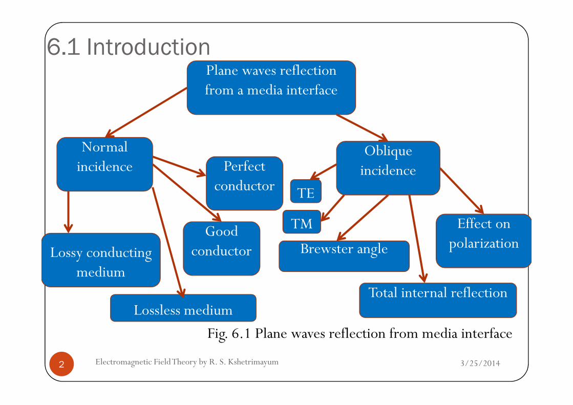
6.1 Introduction Plane waves reflection from a media interface
Normal incidence
TE
Oblique incidencePerfect
conductor
3/25/2014Electromagnetic Field Theory by R. S. Kshetrimayum2
TE
Lossless medium
Good conductor
Fig. 6.1 Plane waves reflection from media interface
Lossy conducting medium
TMBrewster angle
Total internal reflection
Effect on polarization
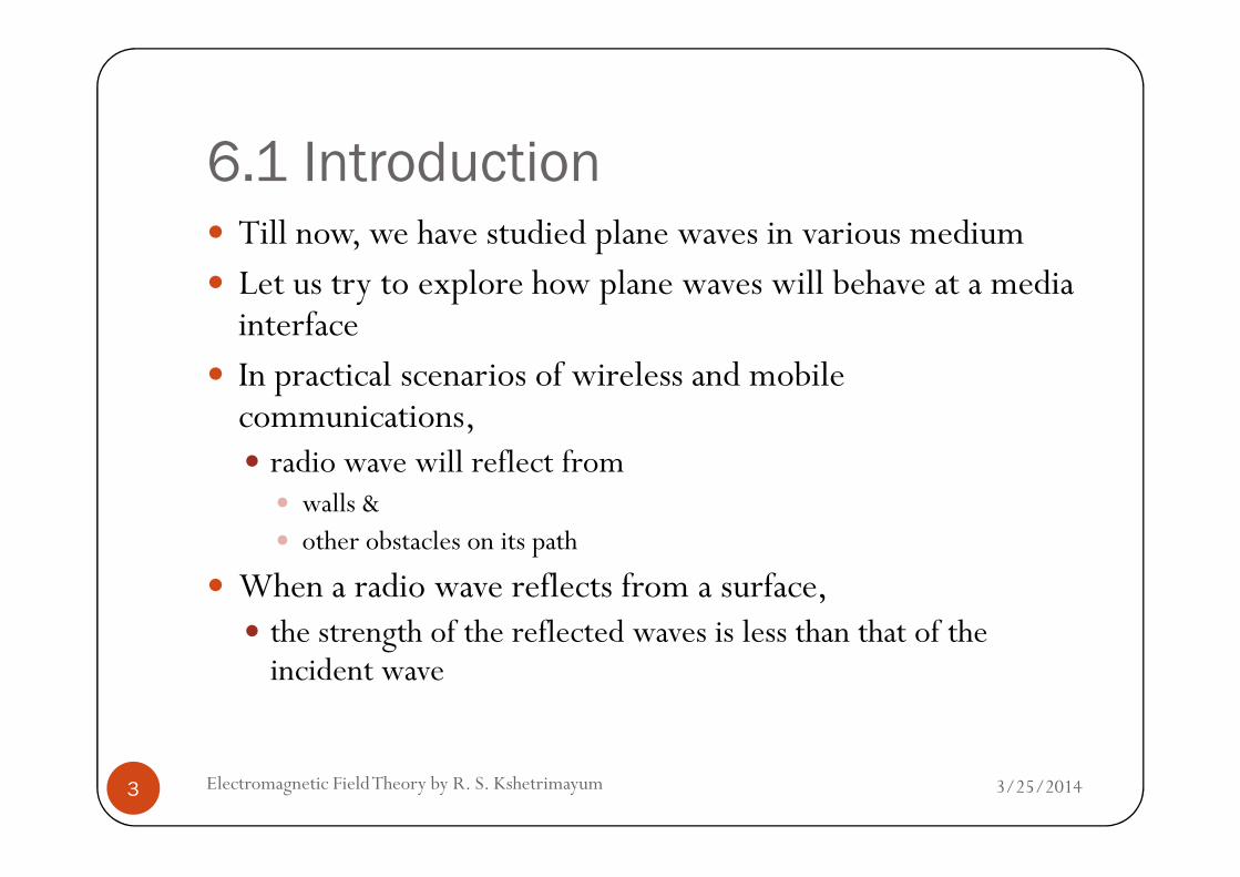
6.1 Introduction� Till now, we have studied plane waves in various medium� Let us try to explore how plane waves will behave at a media interface
� In practical scenarios of wireless and mobile communications, � radio wave will reflect from
� walls & � other obstacles on its path
� When a radio wave reflects from a surface, � the strength of the reflected waves is less than that of the incident wave
3/25/20143 Electromagnetic Field Theory by R. S. Kshetrimayum
6.1 Introduction� The ratio of the two (reflected wave/incident wave) is known as the ‘reflection coefficient’ of the surface
� This ratio depends on the � conductivity (σ), � permittivity (ε) and
3/25/2014Electromagnetic Field Theory by R. S. Kshetrimayum4
� permittivity (ε) and � permeability (µ)
� of the material that forms the reflective surface � as well as material properties of the
� air
� from which the radio wave is incident
6.1 Introduction� Some part of the wave will be transmitted through the material
� How much of the incident wave has been transmitted through the material is � also dependent on the material parameters mentioned above
3/25/2014Electromagnetic Field Theory by R. S. Kshetrimayum5
� also dependent on the material parameters mentioned above� It is given by another ratio known as ‘transmission coefficient’
� It is the ratio of the transmitted wave divided by the incident wave

6.1 Introduction� In plane wave reflection from media interface, � what we will be doing is
� basically writing down the � electric and � magnetic field expressions
3/25/2014Electromagnetic Field Theory by R. S. Kshetrimayum6
� magnetic field expressions
� in all the regions of interest and � apply the boundary conditions
� to get the values of the � transmission and � reflection coefficients
6.1 Introduction� One of the possible applications of such an exercise is in wireless communication, � where we have to find the
� transmission and � reflection coefficients of
� multipaths
3/25/2014Electromagnetic Field Theory by R. S. Kshetrimayum7
� multipaths� Electromagnetic waves are often
� reflected or � scattered or � diffracted
� at one or more obstacles before arriving at the receiver
6.2 Plane wave reflection from media
interface at normal incidence
� For smooth surfaces, � EM waves are reflected;
� For rough surfaces, � EM waves are scattered;
� For edges of surfaces,
3/25/2014Electromagnetic Field Theory by R. S. Kshetrimayum8
� For edges of surfaces, � EM waves are diffracted
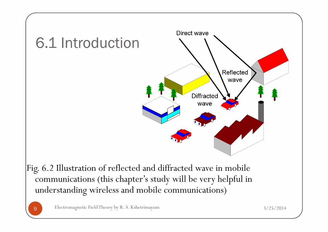
� Fig. 6.2 depicts multipath for a mobile receiver in the car from � direct, � reflected and � diffracted waves
� of the signal sent from the base station
6.1 Introduction
3/25/2014Electromagnetic Field Theory by R. S. Kshetrimayum9
Fig. 6.2 Illustration of reflected and diffracted wave in mobile communications (this chapter’s study will be very helpful in understanding wireless and mobile communications)
6.2 Plane wave reflection from media
interface at normal incidence
� We will consider the case of normal incidence, � when the incident wave propagation vector is along the normal to the interface between two media
6.2.1 Lossy conducting medium
� We will assume plane waves with electric field vector
3/25/2014Electromagnetic Field Theory by R. S. Kshetrimayum10
� We will assume plane waves with electric field vector oriented along the x-axis and
� propagating along the positive z-axis without loss of generality
� For z<0 (we will refer this region as region I and it is assumed to be a lossy medium)
6.2 Plane wave reflection from media
interface at normal incidence
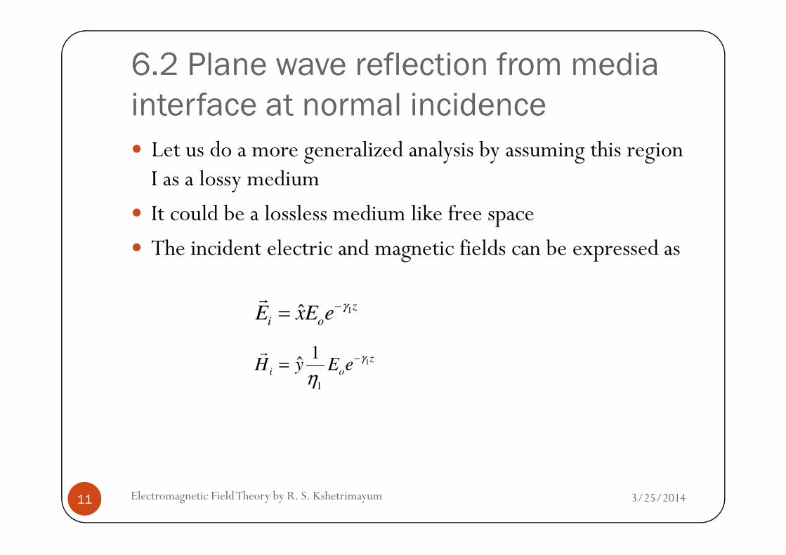
� Let us do a more generalized analysis by assuming this region I as a lossy medium
� It could be a lossless medium like free space� The incident electric and magnetic fields can be expressed as
3/25/2014Electromagnetic Field Theory by R. S. Kshetrimayum11
1ˆ z
i oE xE e
γ−=r
1
1
1ˆ z
i oH y E e
γ
η−=
r

6.2 Plane wave reflection from media
interface at normal incidence
� where η1 is the medium 1 wave impedance and � Eo is the arbitrary amplitude of the incident electric field� The expression for intrinsic wave impedance and propagation constant
3/25/2014Electromagnetic Field Theory by R. S. Kshetrimayum12
( )1 1 1 1
1 1 1 1 1 1
1 1 1 11 1 1
; 1j j j j
j jjj j
ωµ ωµ ωµ ση γ α β ω µ ε
γ ωε σ ωεωµ ωε σ= = = = + = −
++
6.2 Plane wave reflection from media
interface at normal incidence
iEr
Er
2
tγr
1
iγr
iHr
tEr
tHr
iEr
r
3/25/2014Electromagnetic Field Theory by R. S. Kshetrimayum13
2 2 2, ,ε µ σ
rEr
1 1 1, ,ε µ σ
1
rγr
rHrr
Er
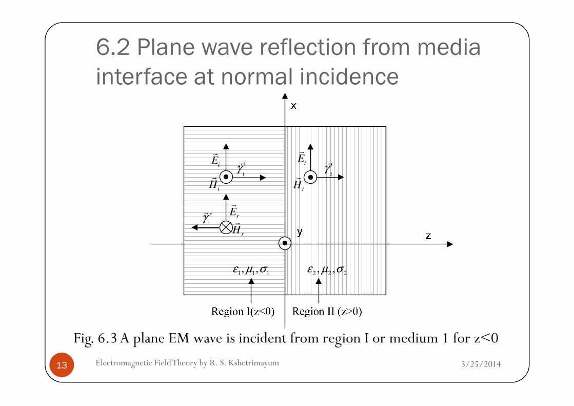
Fig. 6.3 A plane EM wave is incident from region I or medium 1 for z<0

6.2 Plane wave reflection from media
interface at normal incidence
� Convention: � a circle with a dot in the center � an arrow pointing perpendicularly out of the page and
� a circle with a cross � an arrow pointing perpendicularly into the page)
3/25/2014Electromagnetic Field Theory by R. S. Kshetrimayum14
the page)
� Notation for fields: � subscript i� incident, r� reflected and t�transmitted
6.2 Plane wave reflection from media
interface at normal incidence
� Note that the incident wave from region I will be partially reflected and transmitted at the media interface between two regions
� For reflected wave, z<0, wave direction is in the –z axis and the reflected electric field is expressed as
3/25/2014Electromagnetic Field Theory by R. S. Kshetrimayum15
the reflected electric field is expressed as
� where the Γ is the reflection coefficient
1ˆ z
r oE x E e
γ+= Γr

6.2 Plane wave reflection from media
interface at normal incidence
� The reflection coefficient is defined as the ratio of amplitude of the reflected electric field divided by amplitude of the incident electric field as follows:
r
i
E
EΓ =
3/25/2014Electromagnetic Field Theory by R. S. Kshetrimayum16
� The reflected magnetic field can be obtained from the reflected electric field using the Maxwell’s curl equations as
iE

6.2 Plane wave reflection from media
interface at normal incidence
1
1
1 1 1
ˆ ˆ ˆ
0 0
r r
r r
r
z
o
E j H
x y z
E j E jH
j x y z
E eγ
ωµ
ωµ ωµ ωµ+
∇× = −
∇× ∇× ∂ ∂ ∂⇒ = − = =
∂ ∂ ∂
Γ
r r
r rr
3/25/2014Electromagnetic Field Theory by R. S. Kshetrimayum17
( ) ( ) ( )1 1 11
1
1 1 1
0 0
ˆ ˆ ˆ
o
z z z
o o o
E e
j jy E e y E e y E e
z j
γ γ γγγ
ωµ ωµ ωµ+ + +
Γ
∂ = Γ = Γ = − Γ
∂
1
1
ˆ z
r oH y E e
γ
η+Γ
∴ = −r

6.2 Plane wave reflection from media
interface at normal incidence
� Therefore, the Poynting vector for reflected wave of region I is
� shows power is traveling in the -z axis for the reflected wave
2 2* 2
*
1
ˆz
r r r o
zS E H E e
α
η+= × == − Γ
r r r
3/25/2014Electromagnetic Field Theory by R. S. Kshetrimayum18
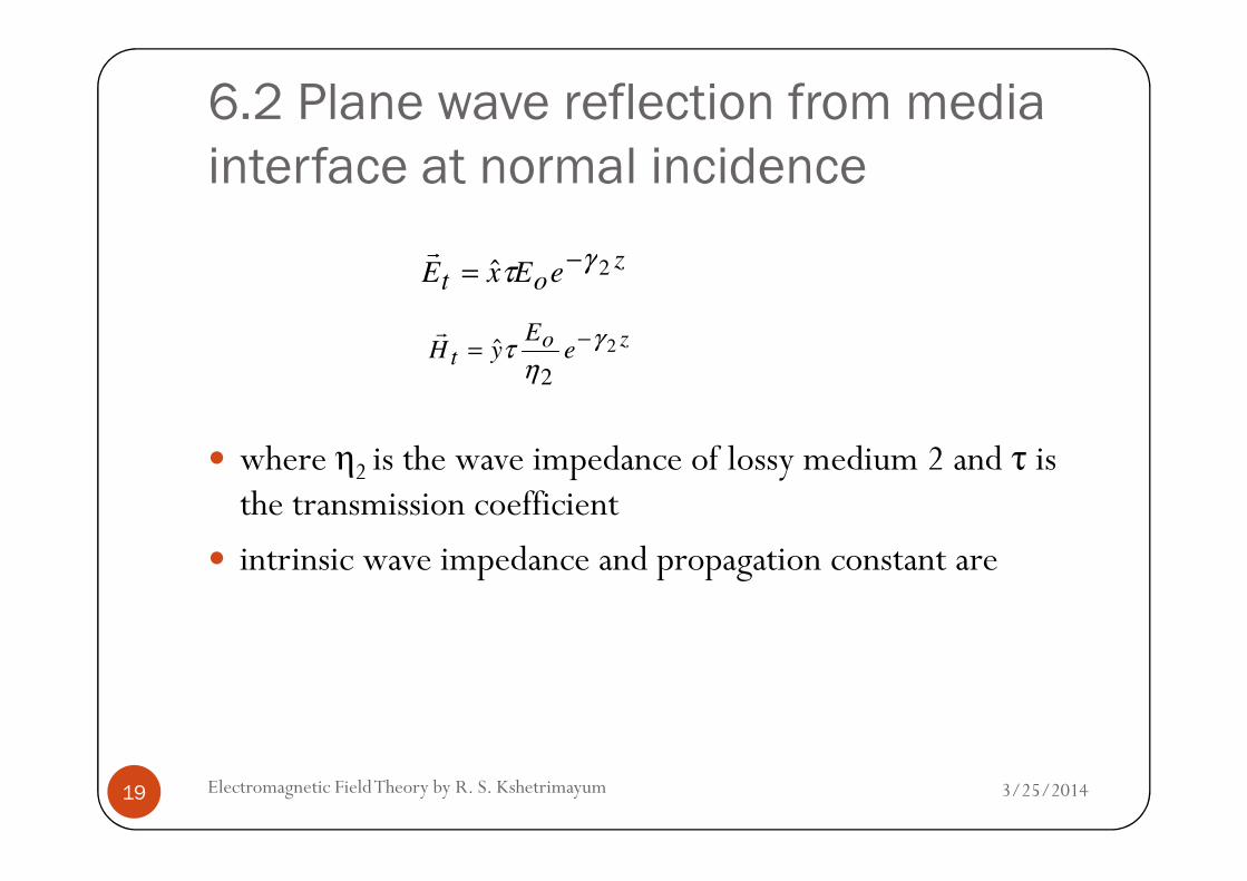
� shows power is traveling in the -z axis for the reflected wave� For transmitted wave, z>0, wave is propagating in lossymedium 2 (we will refer this region as region II),
6.2 Plane wave reflection from media
interface at normal incidence
where η is the wave impedance of lossy medium 2 and τ is
zot eExE 2ˆ γτ −=
r
zot e
EyH 2
2
ˆ γ
ητ −=
r
3/25/2014Electromagnetic Field Theory by R. S. Kshetrimayum19
� where η2 is the wave impedance of lossy medium 2 and τ is the transmission coefficient
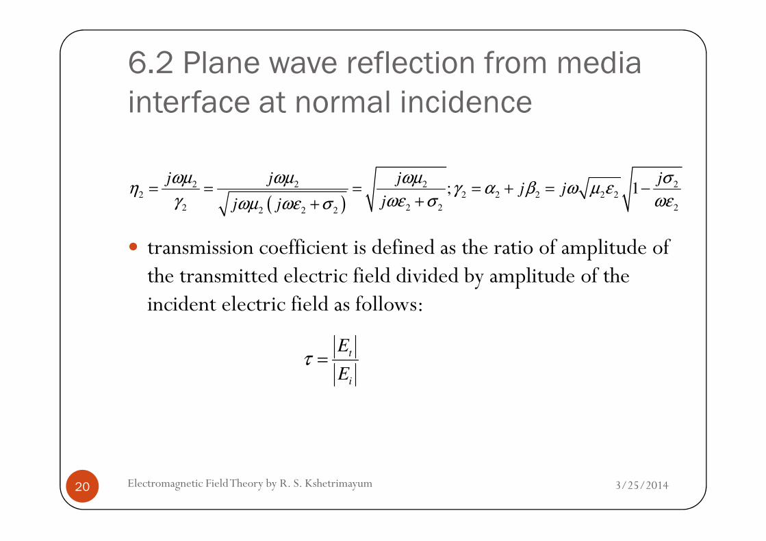
� intrinsic wave impedance and propagation constant are
6.2 Plane wave reflection from media
interface at normal incidence
� transmission coefficient is defined as the ratio of amplitude of the transmitted electric field divided by amplitude of the
( )2 2 2 2
2 2 2 2 2 2
2 2 2 22 2 2
; 1j j j j
j jjj j
ωµ ωµ ωµ ση γ α β ω µ ε
γ ωε σ ωεωµ ωε σ= = = = + = −
++
3/25/2014Electromagnetic Field Theory by R. S. Kshetrimayum20
the transmitted electric field divided by amplitude of the incident electric field as follows:
t
i
E
Eτ =
6.2 Plane wave reflection from media
interface at normal incidence
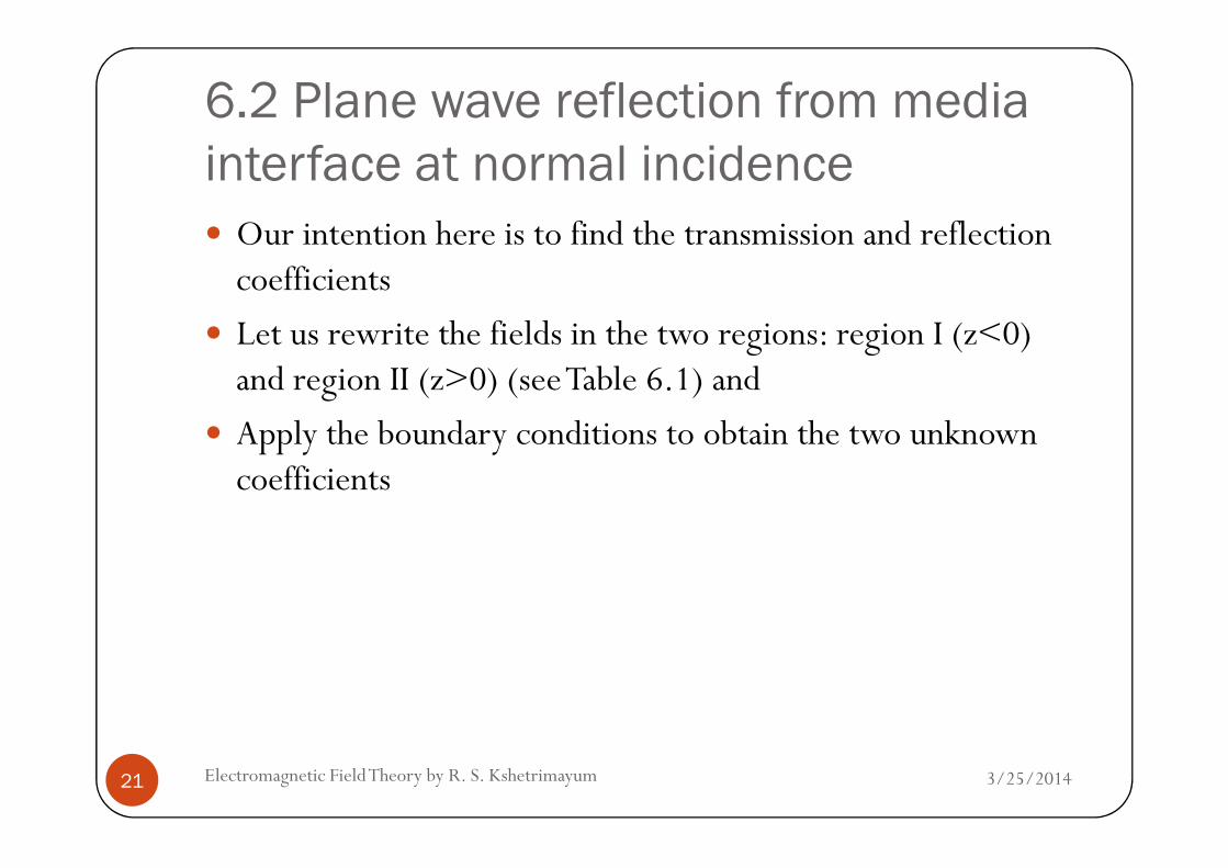
� Our intention here is to find the transmission and reflection coefficients
� Let us rewrite the fields in the two regions: region I (z<0) and region II (z>0) (see Table 6.1) and
� Apply the boundary conditions to obtain the two unknown
3/25/2014Electromagnetic Field Theory by R. S. Kshetrimayum21
� Apply the boundary conditions to obtain the two unknown coefficients

6.2 Plane wave reflection from media
interface at normal incidence
Region I (lossy medium 1) Region II (lossy medium 2)
Table 6.1 Fields in the two lossy regions (normal incidence)
3/25/2014Electromagnetic Field Theory by R. S. Kshetrimayum22
1ˆ z
i oE xE e
γ−=r
1
1
1ˆ z
i oH y E e
γ
η−=
r
1ˆ z
r oE x E e
γ+= Γr
1
1
ˆ z
r oH y E e
γ
η+Γ
= −r
zot eExE 2ˆ γτ −=
r zot e
EyH 2
2
ˆ γ
ητ −=
r
6.2 Plane wave reflection from media
interface at normal incidence
� This is basically boundary value problem with boundary conditions at z=0
� Note that total electric and magnetic fields (both incident and reflected) are tangential to the interface at z=0
� Similarly, the transmitted electric and magnetic field are also
3/25/2014Electromagnetic Field Theory by R. S. Kshetrimayum23
� Similarly, the transmitted electric and magnetic field are also tangential to the interface at z=0
� Also note that there are no surface current density at the interface
� Hence, the tangential components of electric and magnetic fields must be continuous at the interface z=0
6.2 Plane wave reflection from media
interface at normal incidence
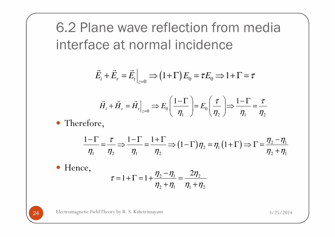
Therefore,
( ) 0 00
1 1i r t
zE E E E Eτ τ
=+ = ⇒ + Γ = ⇒ + Γ =
r r r
0 00
1 2 1 2
1 1i r t
zH H H E E
τ τ
η η η η=
− Γ − Γ+ = ⇒ = ⇒ =
r r r
3/25/2014Electromagnetic Field Theory by R. S. Kshetrimayum24
� Therefore,
� Hence,
( ) ( ) 2 1
2 1
1 2 1 2 2 1
1 1 11 1
η ητη η
η η η η η η
−− Γ − Γ + Γ= ⇒ = ⇒ − Γ = + Γ ⇒ Γ =
+
2 1 2
2 1 1 2
21 1
η η ητ
η η η η
−= + Γ = + =
+ +
6.2 Plane wave reflection from media
interface at normal incidence
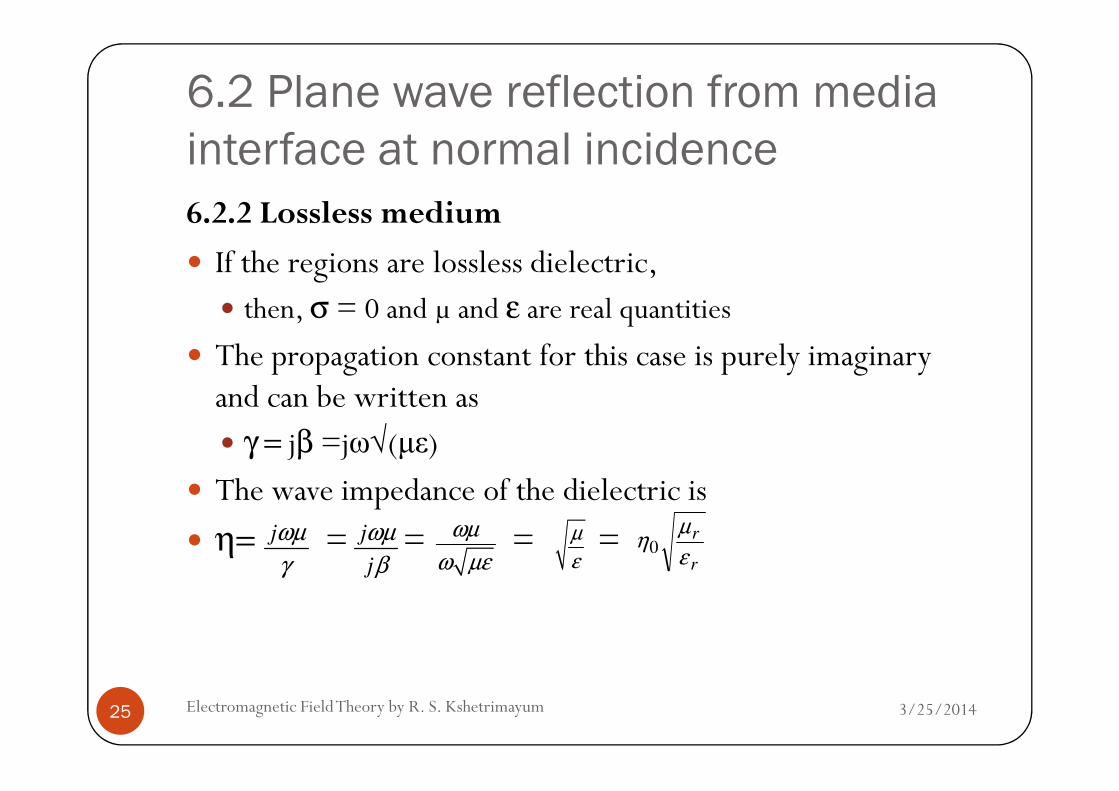
6.2.2 Lossless medium
� If the regions are lossless dielectric, � then, σ = 0 and µ and ε are real quantities
� The propagation constant for this case is purely imaginary and can be written as
3/25/2014Electromagnetic Field Theory by R. S. Kshetrimayum25
and can be written as � γ = jβ =jω√(µε)
� The wave impedance of the dielectric is � η= = = = = jωµ
γ
j
j
ωµ
β
ωµ
ω µε
µ
ε r
r
ε
µη0

6.2 Plane wave reflection from media
interface at normal incidence
� For a lossless medium, � η is real, so, � both Γ and τ are real� Electric and magnetic fields are in phase with each otherThe wavelength in the dielectric is
3/25/2014Electromagnetic Field Theory by R. S. Kshetrimayum26
� The wavelength in the dielectric is� = =� And the phase velocity is� = = =� where c is the speed of light in free space
λ2π
β
2π
ω µε
pvω
β µε
1
rr
c
εµ

6.2 Plane wave reflection from media
interface at normal incidence
Table 6.2 Fields in the two lossless regions (normal incidence)
Region I (lossless medium 1) Region II (lossless medium 2)
3/25/2014Electromagnetic Field Theory by R. S. Kshetrimayum27
1ˆ j z
i oE xE e
β−=r
1
1
1ˆ j z
i oH y E e
β
η−=
r
1ˆ j z
r oE x E e
β+= Γr
1
1
ˆ j z
r oH y E e
β
η+Γ
= −r
2ˆ j z
t oE x E e
βτ −=r
2
2
ˆ j zo
t
EH y e
βτη
−=r
6.2 Plane wave reflection from media
interface at normal incidence
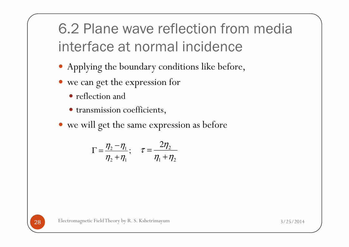
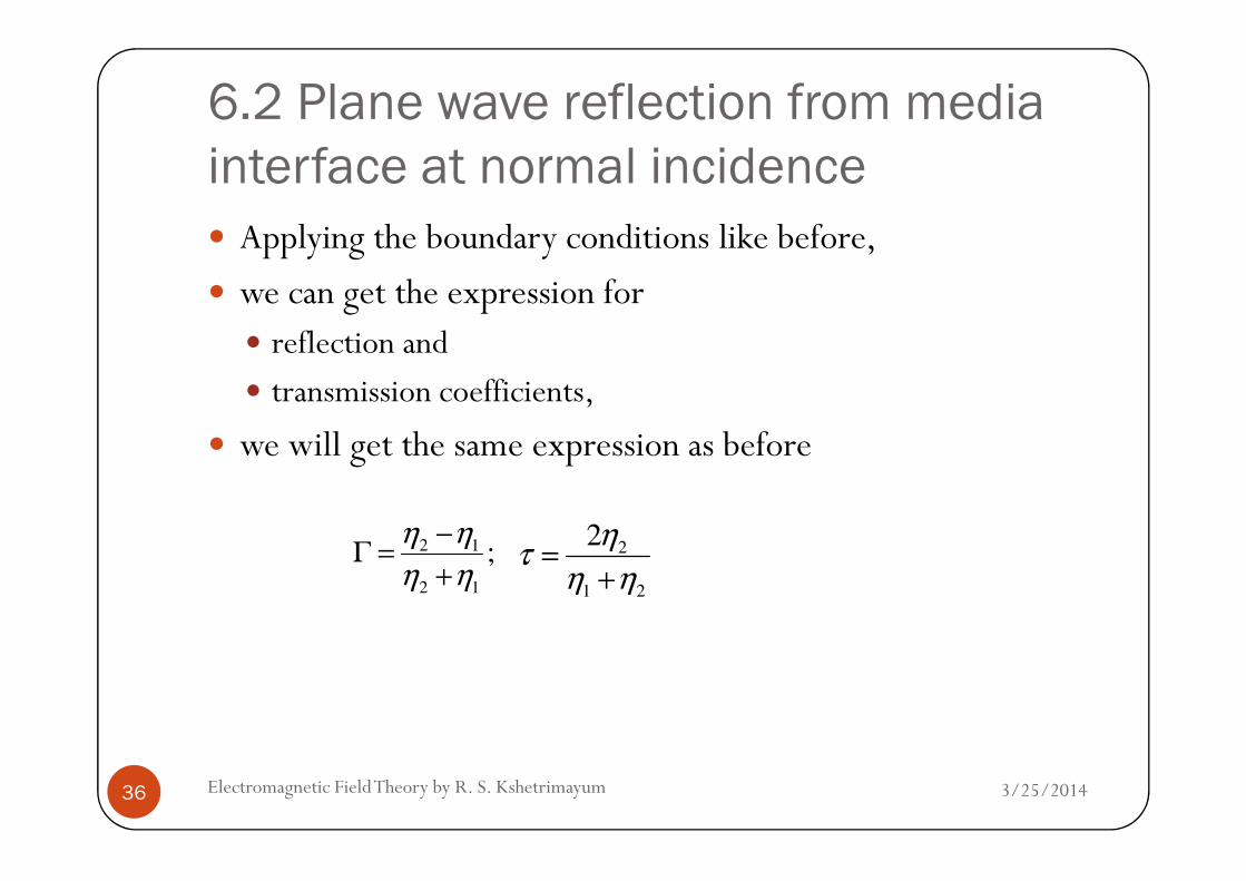
� Applying the boundary conditions like before, � we can get the expression for
� reflection and � transmission coefficients,
� we will get the same expression as before
3/25/2014Electromagnetic Field Theory by R. S. Kshetrimayum28
� we will get the same expression as before
2 1
2 1
;η η
η η
−Γ =
+
2
1 2
2ητ
η η=
+
6.2 Plane wave reflection from media
interface at normal incidence
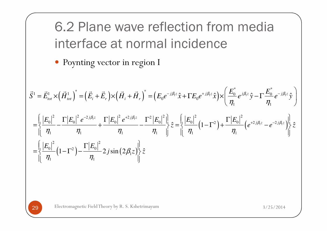
� Poynting vector in region I
( ) ( ) ( ) ( )1 1 1 1
* ** *
1 1 1 0 0
0 0
1 1
ˆ ˆ ˆ ˆj z j z j z j z
tot tot i r i r
E ES E H E E H H E e x E e x e y e y
β β β β
η η− + −
= × = + × + = + Γ × − Γ
r r r r r r r
2 2 2 2 2 22 2 2j z j zβ β− + Γ Γ Γ Γ
3/25/2014Electromagnetic Field Theory by R. S. Kshetrimayum29
( ) ( )
( ) ( )
1 1
1 1
2 2 2 2 2 22 2 2
0 0 0 0 0 0 2 22
1 1 1 1 1 1
2 2
0 02
1
1 1
ˆ ˆ1
ˆ1 2 sin 2
j z j z
j z j zE E e E e E E E
z e e z
E Ej z z
β β
β β
η η η η η η
βη η
− +
+ − Γ Γ Γ Γ
= − + − = − Γ + −
Γ = − Γ −
6.2 Plane wave reflection from media
interface at normal incidence
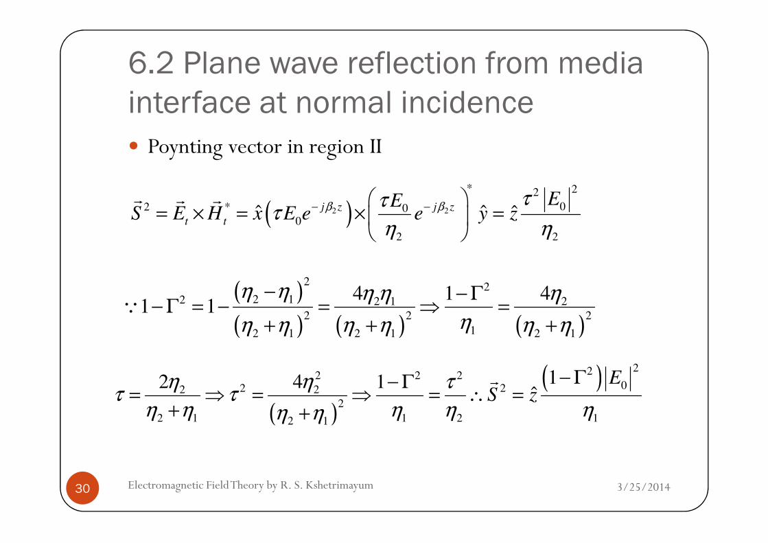
� Poynting vector in region II
( )2 2
* 22
02 * 0
0
2 2
ˆ ˆ ˆj z j z
t t
EES E H x E e e y z
β β τττ
η η− −
= × = × =
r r r
3/25/2014Electromagnetic Field Theory by R. S. Kshetrimayum30
( )
( ) ( ) ( )
22
2 12 2 1 2
2 2 2
12 1 2 1 2 1
4 411 1
η η η η η
ηη η η η η η
− − Γ− Γ = − = ⇒ =
+ + +Q
( )
( ) 222 2 202 22 2
2
2 1 1 2 12 1
12 4 1ˆ
ES z
η η ττ τ
η η η η ηη η
− Γ− Γ= ⇒ = ⇒ = ∴ =
+ +
r

6.2 Plane wave reflection from media
interface at normal incidence
Power conservation
� Compare the time average power flow in the two regions� For z <0, the time average power flow through 1m2 cross section is
( )2
1 1 1− Γr
3/25/2014Electromagnetic Field Theory by R. S. Kshetrimayum31
� And for z >0, the time average power flow through 1m2
cross section is
( )2
21 1
0
1
1 1 1ˆRe
2 2avg
S S z Eη
− Γ= • =
r
( )2
22 2
0
1
1 1 1ˆRe
2 2avg
S S z Eη
− Γ= • =
r

6.2 Plane wave reflection from media
interface at normal incidence
� Hence,
� So real power is conserved6.2.3 Good conductor:
If the region II (z >0) is a good (but not perfect) conductor
1 2
avg avgS S=
3/25/2014Electromagnetic Field Theory by R. S. Kshetrimayum32
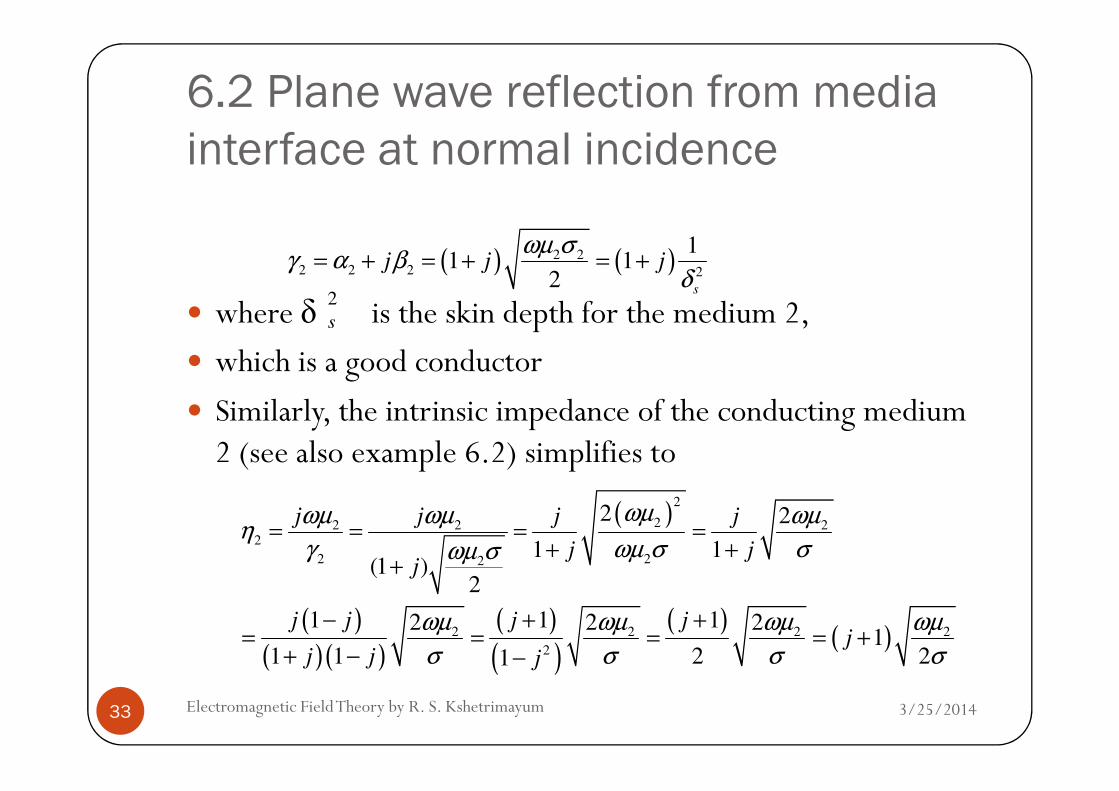
� If the region II (z >0) is a good (but not perfect) conductor and
� region I is a lossless medium like free space, � the propagation constant for medium 2 is
6.2 Plane wave reflection from media
interface at normal incidence
� where δ is the skin depth for the medium 2, � which is a good conductorSimilarly, the intrinsic impedance of the conducting medium
( ) ( )2 2
2 2 2 2
11 1
2s
j j jωµ σ
γ α βδ
= + = + = +
2
s
3/25/2014Electromagnetic Field Theory by R. S. Kshetrimayum33
� Similarly, the intrinsic impedance of the conducting medium 2 (see also example 6.2) simplifies to
( )
( )( )( )
( )
( )( )
( )
2
22 2 2
2
2 22
2 2 2 2
2
2 2
1 1(1 )
2
1 1 12 2 21
1 1 2 21
j j j j
j jj
j j j jj
j j j
ωµωµ ωµ ωµη
γ ωµ σ σωµ σ
ωµ ωµ ωµ ωµ
σ σ σ σ
= = = =+ +
+
− + += = = = +
+ − −
6.2 Plane wave reflection from media
interface at normal incidence
� Now, the wave impedance of medium 2 is complex, with a phase angle of 45o so the electric
� and magnetic field will be 45o out of phase and Γ and τ will be complex.
� Now, let us write down the field expressions in region I and
3/25/2014Electromagnetic Field Theory by R. S. Kshetrimayum34
� Now, let us write down the field expressions in region I and II for lossless dielectric (region I) and good conductor (region II) interface

6.2 Plane wave reflection from media
interface at normal incidence
Table 6.4 Fields in the two regions (normal incidence)
Region I (lossless medium) Region II (good conductor)
3/25/2014Electromagnetic Field Theory by R. S. Kshetrimayum35
1ˆ j z
i oE xE e
β−=r
1
1
1ˆ j z
i oH y E e
β
η−=
r
1ˆ j z
r oE x E e
β+= Γr
1
1
ˆ j z
r oH y E e
β
η+Γ
= −r
2ˆ z
t oE x E e
γτ −=r
2
2
ˆ zo
t
EH y e
γτη
−=r
6.2 Plane wave reflection from media
interface at normal incidence
� Applying the boundary conditions like before, � we can get the expression for
� reflection and � transmission coefficients,
� we will get the same expression as before
3/25/2014Electromagnetic Field Theory by R. S. Kshetrimayum36
� we will get the same expression as before
2 1
2 1
;η η
η η
−Γ =
+2
1 2
2ητ
η η=
+

6.2 Plane wave reflection from media
interface at normal incidence
� Note that we have to use the previous expressions for intrinsic wave impedances for lossless medium and good conductor
1;
µη
ε= ( ) 2
21
2j
ωµη
σ= +
3/25/2014Electromagnetic Field Theory by R. S. Kshetrimayum37
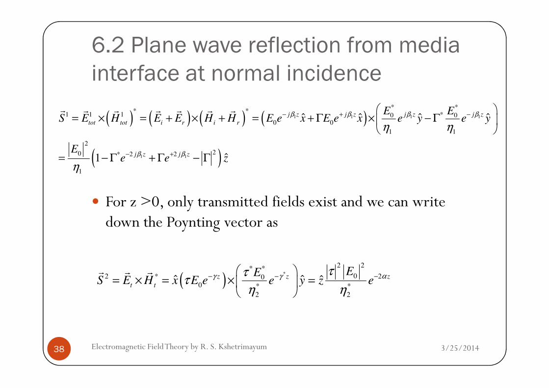
Power conservation
� let us find out the Poynting vector in the two regions� Noting that the field in region I comprise of incident and reflected wave,
� we can write the Poynting vector for z <0
ε ( )2
2
12
jησ
= +
6.2 Plane wave reflection from media
interface at normal incidence
For z >0, only transmitted fields exist and we can write
( ) ( ) ( ) ( )
( )
1 1 1 1
1 1
* ** *
1 1 1 *0 0
0 0
1 1
2
20 2 2*
1
ˆ ˆ ˆ ˆ
ˆ1
j z j z j z j z
tot tot i r i r
j z j z
E ES E H E E H H E e x E e x e y e y
Ee e z
β β β β
β β
η η
η
− + −
− +
= × = + × + = + Γ × − Γ
= − Γ + Γ − Γ
r r r r r r r
3/25/2014Electromagnetic Field Theory by R. S. Kshetrimayum38
� For z >0, only transmitted fields exist and we can write down the Poynting vector as
( )*
2 2* *
02 * 20
0 * *
2 2
ˆ ˆ ˆz z z
t t
EES E H x E e e y z e
γ γ ατττ
η η− − −
= × = × =
r r r
6.2 Plane wave reflection from media
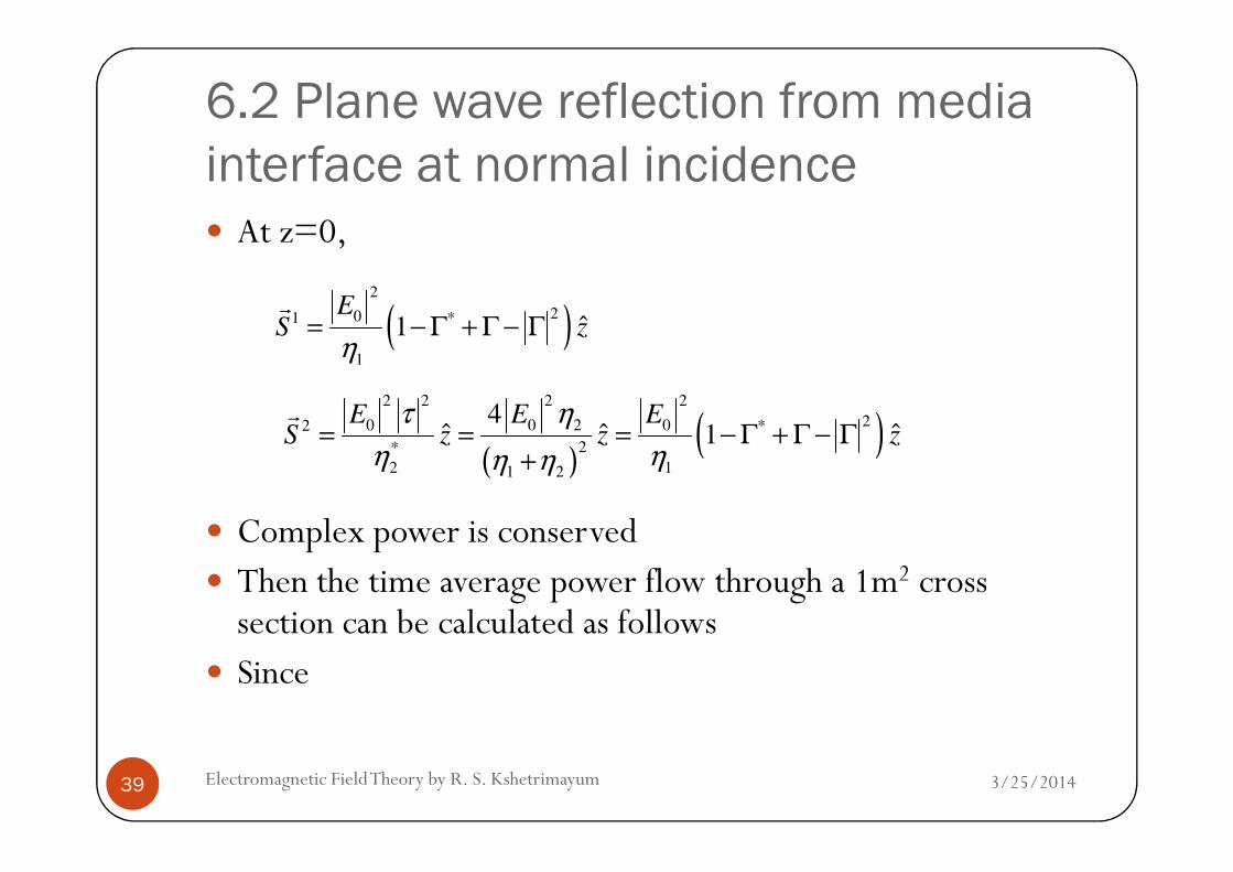
interface at normal incidence� At z=0,
( )2
201 *
1
ˆ1E
S zη
= − Γ + Γ − Γr
( )( )
2 2 2 2
20 0 2 02 *4
ˆ ˆ ˆ1E E E
S z z zτ η
= = = − Γ + Γ − Γr
3/25/2014Electromagnetic Field Theory by R. S. Kshetrimayum39
� Complex power is conserved� Then the time average power flow through a 1m2 cross section can be calculated as follows
� Since
( )( )2*
2 11 2
ˆ ˆ ˆ1S z z zη ηη η
= = = − Γ + Γ − Γ+

6.2 Plane wave reflection from media
interface at normal incidence
� is purely an imaginary number, therefore,
1 12 2* j z j ze e
β β− +−Γ + Γ
( )2
21 1
0
11 1ˆRe
2 2avg
S S z Eη
− Γ= • =
r
3/25/2014Electromagnetic Field Theory by R. S. Kshetrimayum40
� which shows power balance at z=0 only
( ) 0
1
ˆRe2 2
avgS S z E
η= • =
( ) z
avg eEzSSα
η2
2
2
2
0
221
2
1ˆRe
2
1 −Γ−=•=
r
6.2 Plane wave reflection from media
interface at normal incidence
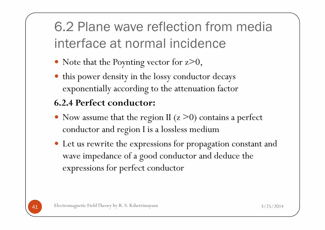
� Note that the Poynting vector for z>0, � this power density in the lossy conductor decays exponentially according to the attenuation factor
6.2.4 Perfect conductor:
� Now assume that the region II (z >0) contains a perfect
3/25/2014Electromagnetic Field Theory by R. S. Kshetrimayum41
� Now assume that the region II (z >0) contains a perfect conductor and region I is a lossless medium
� Let us rewrite the expressions for propagation constant and wave impedance of a good conductor and deduce the expressions for perfect conductor

6.2 Plane wave reflection from media
interface at normal incidence
Perfect conductor implies σ →∝, and
( ) ( )2 2
2 2 2 2
11 1
2s
j j jωµ σ
γ α βδ
= + = + = +
( ) 2
2
2
12
jωµ
ησ
= +
3/25/2014Electromagnetic Field Theory by R. S. Kshetrimayum42
� Perfect conductor implies σ2→∝, and � correspondingly, α2→∝, δs2→0, η2→0� Note that
� Therefore, τ→0 and Γ→-1
2 2 1
1 2 2 1
2,
η η ητ
η η η η
−= Γ =
+ +
6.2 Plane wave reflection from media
interface at normal incidence
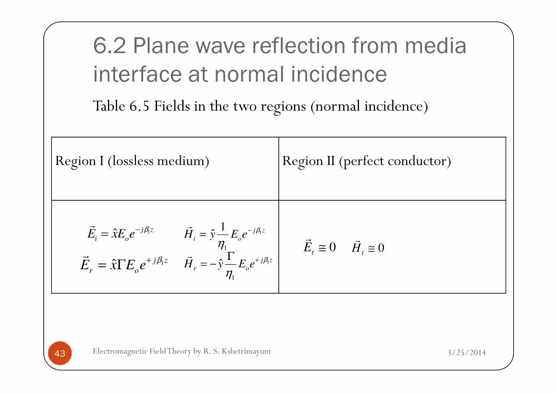
Table 6.5 Fields in the two regions (normal incidence)
Region I (lossless medium) Region II (perfect conductor)
3/25/2014Electromagnetic Field Theory by R. S. Kshetrimayum43
1ˆ j z
i oE xE e
β−=r
1
1
1ˆ j z
i oH y E e
β
η−=
r
1ˆ j z
r oE x E e
β+= Γr
1
1
ˆ j z
r oH y E e
β
η+Γ
= −r
0t
E ≅r
0t
H ≅r

6.2 Plane wave reflection from media
interface at normal incidence
� The field for z >0 thus decay infinitely fast and � are identically zero in the perfect conductor as we have seen in example 6.2 as well
� The perfect conductor can be thought of as ‘shorting out’ the incident electric field
3/25/2014Electromagnetic Field Theory by R. S. Kshetrimayum44
incident electric field� Now let us write down the field expressions in region I and II for lossless dielectric and perfect conductor interface (see Table 6.5)
6.2 Plane wave reflection from media
interface at normal incidence
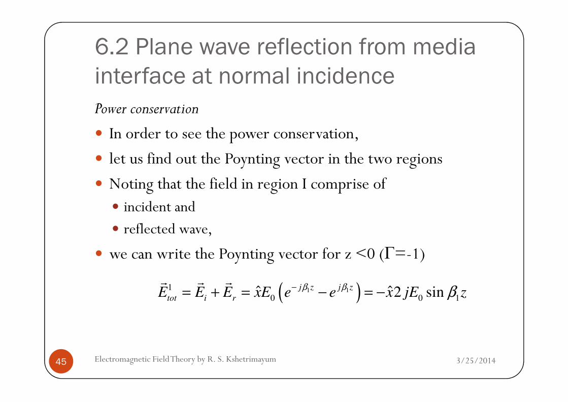
Power conservation
� In order to see the power conservation, � let us find out the Poynting vector in the two regions� Noting that the field in region I comprise of
� incident and
3/25/2014Electromagnetic Field Theory by R. S. Kshetrimayum45
� incident and � reflected wave,
� we can write the Poynting vector for z <0 (Γ=-1)
( )1 11
0 0 1ˆ ˆ2 sin
j z j z
tot i rE E E xE e e x jE z
β β β−= + = − = −r r r

6.2 Plane wave reflection from media
interface at normal incidence
� Therefore, the Poynting vector for z<0 is
( )1 11 0 0
1
1 1
ˆ ˆ2 cosj z j z
tot i r
E EH H H y e e y z
β β βη η
−= + = + =r r
( )2
4 Er r
3/25/2014Electromagnetic Field Theory by R. S. Kshetrimayum46
� which has a zero real part and � thus indicates that no real power is delivered to the perfect conductor� Fields in region II is anyway zero and hence power is also zero
( )2
*01 1 1
1 1
1
4ˆ sin cos
tot tot
ES E H zj z zβ β
η= × = −
r r

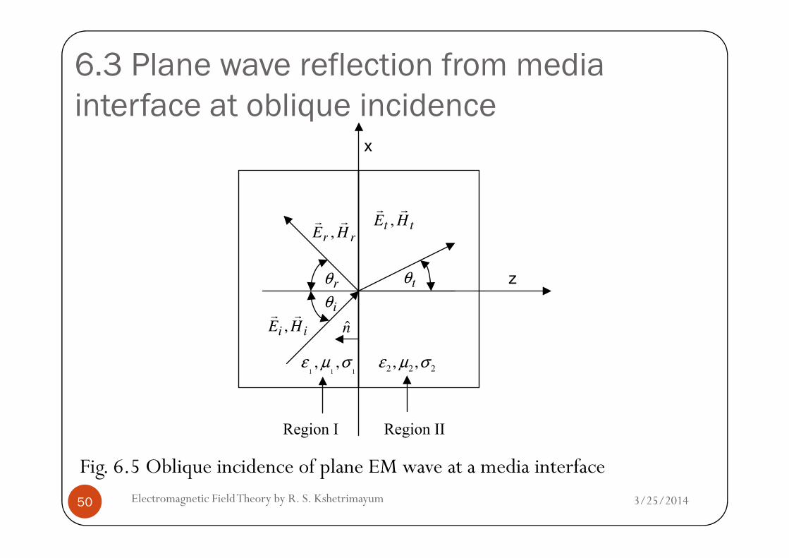
6.3 Plane wave reflection from media
interface at oblique incidence
� We will consider the problem of a plane wave � obliquely incident on a plane interface � between two lossy conducting regions
� We will first consider two particular cases of this problem as follows:
3/25/2014Electromagnetic Field Theory by R. S. Kshetrimayum47
follows:� the electric field is in the xz plane (parallel polarization)� the electric field is in normal to the xz plane (perpendicular polarization)

6.3 Plane wave reflection from media
interface at oblique incidence
� Any arbitrary incident plane wave can be expressed � as a linear combination of these two principal polarizations
� The plane of incidence is that plane containing � the normal vector to the interface and � the direction of propagation vector of the incident wave
3/25/2014Electromagnetic Field Theory by R. S. Kshetrimayum48
� the direction of propagation vector of the incident wave
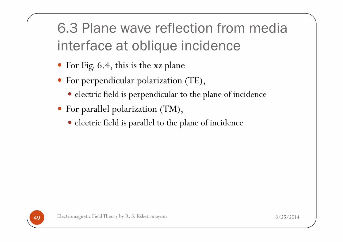
6.3 Plane wave reflection from media
interface at oblique incidence
� For Fig. 6.4, this is the xz plane� For perpendicular polarization (TE),
� electric field is perpendicular to the plane of incidence � For parallel polarization (TM),
� electric field is parallel to the plane of incidence
3/25/2014Electromagnetic Field Theory by R. S. Kshetrimayum49
� electric field is parallel to the plane of incidence
6.3 Plane wave reflection from media
interface at oblique incidence
tt HErr
,
z
x
rr HErr
,
rθ tθ
3/25/2014Electromagnetic Field Theory by R. S. Kshetrimayum50
Fig. 6.5 Oblique incidence of plane EM wave at a media interface
1 1 1, ,ε µ σ
2 2 2, ,ε µ σ
z
Region II
ii HErr
,
Region I
iθrθ tθ
n
6.3 Plane wave reflection from media
interface at oblique incidence
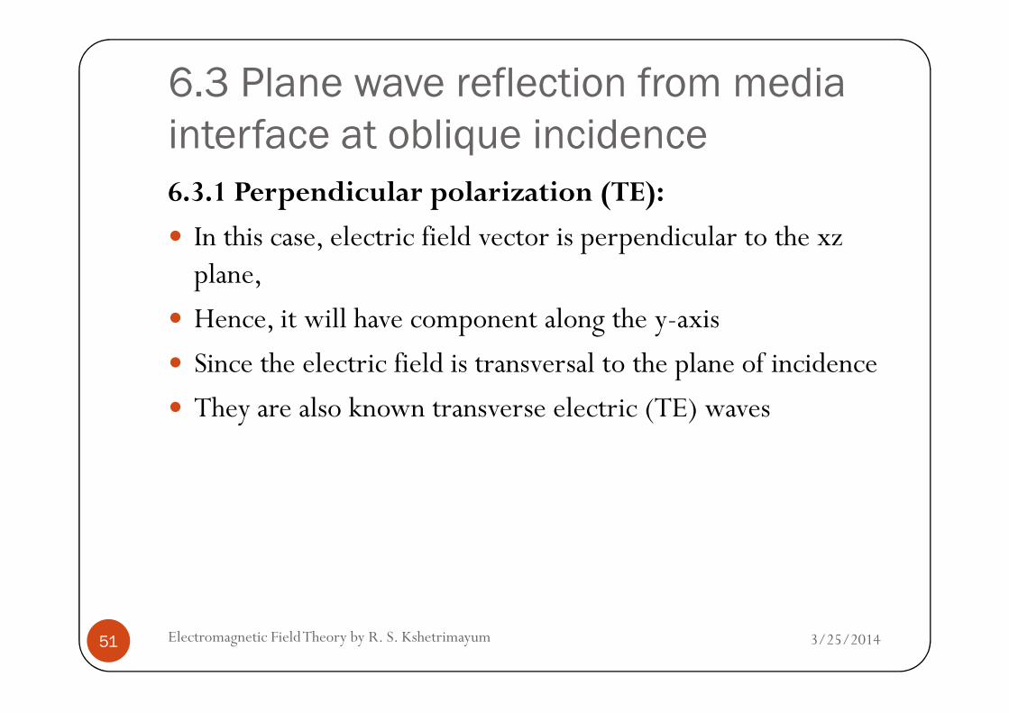
6.3.1 Perpendicular polarization (TE):
� In this case, electric field vector is perpendicular to the xzplane,
� Hence, it will have component along the y-axis� Since the electric field is transversal to the plane of incidence
3/25/2014Electromagnetic Field Theory by R. S. Kshetrimayum51
� Since the electric field is transversal to the plane of incidence� They are also known transverse electric (TE) waves

iθ rθn n z
xx
z
iθγ cos1
iθγ sin1
rθγ cos1
rθγ sin11
iγr
1
rγr
x
3/25/2014Electromagnetic Field Theory by R. S. Kshetrimayum52
tθn z
2cos
tγ θ
2sin tγ θ 2
tγr
Fig. 6.6 Wave propagation vector for (a) incident (b) reflected and (c) transmitted EM waves at oblique incidence

6.3 Plane wave reflection from media
interface at oblique incidence
� Let us assume that the incident wave propagates in the first quadrant of xz plane without loss of generality and
� (incident propagation vector) makes an angle θi with the normal (see Fig. 6.6 (a))
1
iγr
3/25/2014Electromagnetic Field Theory by R. S. Kshetrimayum53
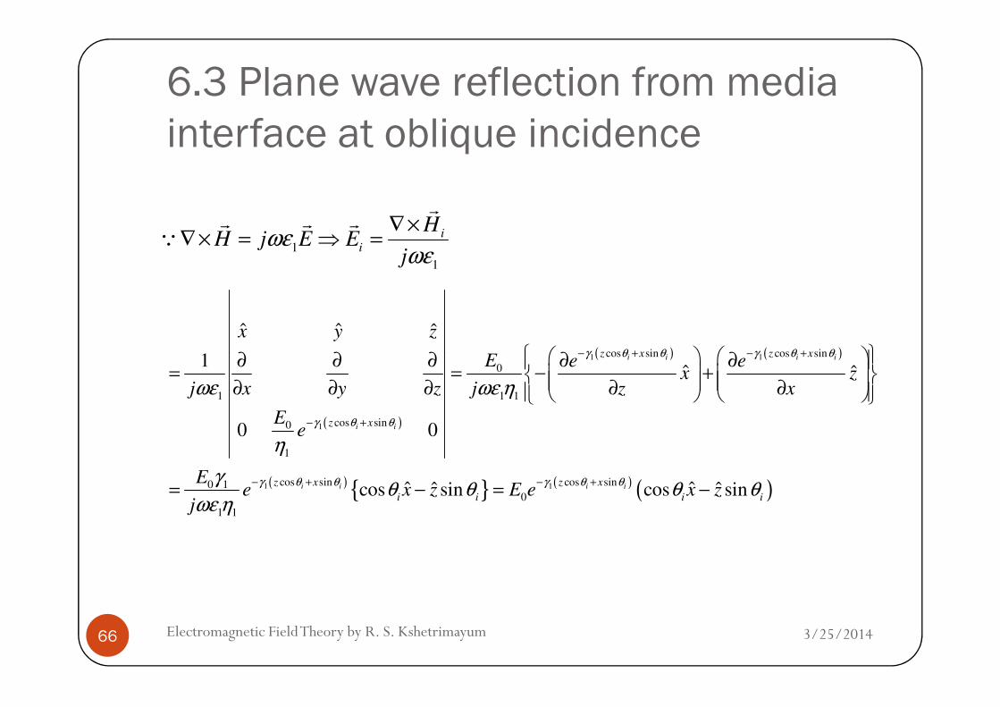
( ) ( ) ( )'
1 1 1 1 1 1ˆ ˆˆ ˆcos sin cos sin cos sin
i
i i i i i iz z x zz xx z x z xγ γ θ γ θ γ θ γ θ γ θ θ• = + • + = + = +
r r
( )1 cos sin
0ˆi iz x
iE E e y
γ θ θ− +=
r
1
1
i
i i i
EE j H H
jωµ
ωµ
∇×∇× = − ⇒ =
−
rr r r
Q
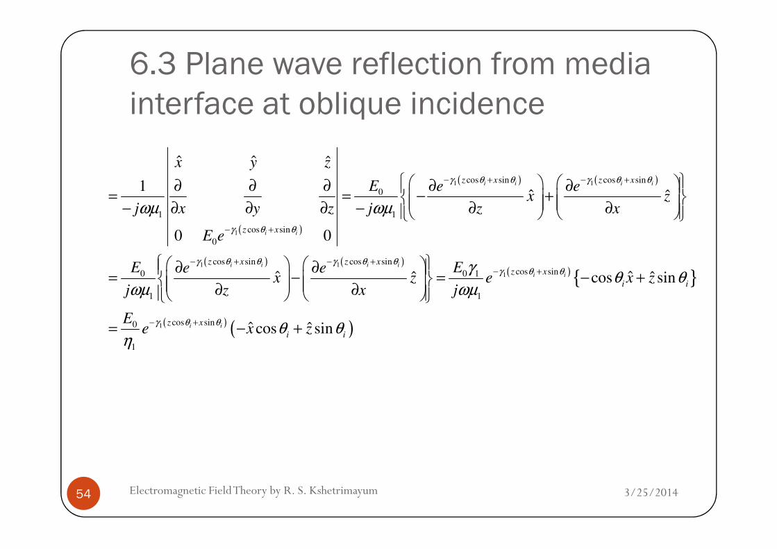
6.3 Plane wave reflection from media
interface at oblique incidence
( )
( ) ( )
( ) ( )
1 1
1
1 1
cos sin cos sin
0
1 1
cos sin
0
cos sin cos sin
0
ˆ ˆ ˆ
1ˆ ˆ
0 0
ˆ ˆ
i i i i
i i
i i i i
z x z x
z x
z x z x
x y z
E e ex z
j x y z j z x
E e
E e ex z
γ θ θ γ θ θ
γ θ θ
γ θ θ γ θ θ
ωµ ωµ
− + − +
− +
− + − +
∂ ∂ ∂ ∂ ∂ = = − + − ∂ ∂ ∂ − ∂ ∂
∂ ∂ = −
( ) { }1 cos sin0 1 ˆ ˆcos sini iz xEe x z
γ θ θγθ θ− +
= − +
3/25/2014Electromagnetic Field Theory by R. S. Kshetrimayum54
0
1
ˆ ˆE e e
x zj z xωµ
∂ ∂ = − ∂ ∂
( ) { }
( ) ( )
1
1
cos sin0 1
1
cos sin0
1
ˆ ˆcos sin
ˆ ˆcos sin
i i
i i
z x
i i
z x
i i
Ee x z
j
Ee x z
γ θ θ
γ θ θ
γθ θ
ωµ
θ θη
− +
− +
= − +
= − +
6.3 Plane wave reflection from media
interface at oblique incidence
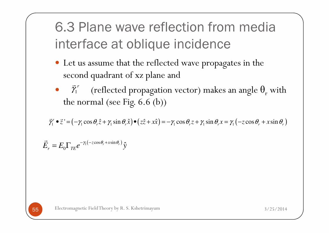
� Let us assume that the reflected wave propagates in the second quadrant of xz plane and
� (reflected propagation vector) makes an angle θr with the normal (see Fig. 6.6 (b))
1
rγr
3/25/2014Electromagnetic Field Theory by R. S. Kshetrimayum55
( ) ( ) ( )1 1 1 1 1 1ˆ ˆˆ ˆ' cos sin cos sin cos sin
r
r r r r r rz z x zz xx z x z xγ γ θ γ θ γ θ γ θ γ θ θ• = − + • + = − + = − +
r r
( )1 cos sin
0ˆr rz x
r TEE E e y
γ θ θ− − += Γ
r

6.3 Plane wave reflection from media
interface at oblique incidence
� Note that and will have the same magnitude � since both the waves are still in the same region I, � only their direction changes
� Since the Poynting vector must be negative like the previous case of normal incidence,
1
rγr
1
iγr
3/25/2014Electromagnetic Field Theory by R. S. Kshetrimayum56
case of normal incidence,
� You could also use the Maxwell’s curl equation below to find this
( ) ( )1 cos sin0
1
ˆ ˆcos sinr rz x
r TE r r
EH e x z
γ θ θ θ θη
− − += Γ +
r
1ωµj
EH r
r−
×∇=
rr
6.3 Plane wave reflection from media
interface at oblique incidence
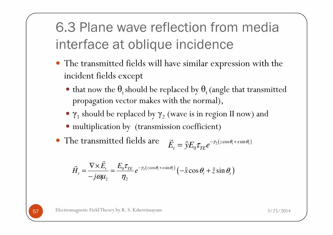
� The transmitted fields will have similar expression with the incident fields except� that now the θi should be replaced by θt (angle that transmitted propagation vector makes with the normal),
� γ1 should be replaced by γ2 (wave is in region II now) and
3/25/2014Electromagnetic Field Theory by R. S. Kshetrimayum57
� γ1 should be replaced by γ2 (wave is in region II now) and� multiplication by (transmission coefficient)
� The transmitted fields are ( )2 cos sin
0ˆ t tz x
t TEE yE e
γ θ θτ − +=
r
( ) ( )2 cos sin0
2 2
ˆ ˆcos sint tz xt TE
t t t
E EH e x z
j
γ θ θτθ θ
ωµ η
− +∇×= = − +
−
rr
6.3 Plane wave reflection from media
interface at oblique incidence
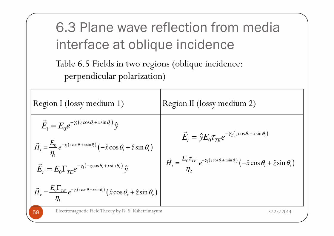
Table 6.5 Fields in two regions (oblique incidence: perpendicular polarization)
Region I (lossy medium 1) Region II (lossy medium 2)
3/25/2014Electromagnetic Field Theory by R. S. Kshetrimayum58
( )1 cos sin
0ˆi iz x
iE E e y
γ θ θ− +=
r
( ) ( )1 cos sin0
1
ˆ ˆcos sini iz x
i i i
EH e x z
γ θ θ θ θη
− += − +
r
( )1 cos sin
0ˆr rz x
r TEE E e y
γ θ θ− − += Γ
r
( ) ( )1 cos sin0
1
ˆ ˆcos sini iz xTE
r r r
EH e x z
γ θ θ θ θη
− +Γ= +
r
( )2 cos sin
0ˆ t tz x
t TEE yE e
γ θ θτ − +=
r
( ) ( )2 cos sin0
2
ˆ ˆcos sint tz xTE
t t t
EH e x z
γ θ θτθ θ
η
− += − +
r
6.3 Plane wave reflection from media
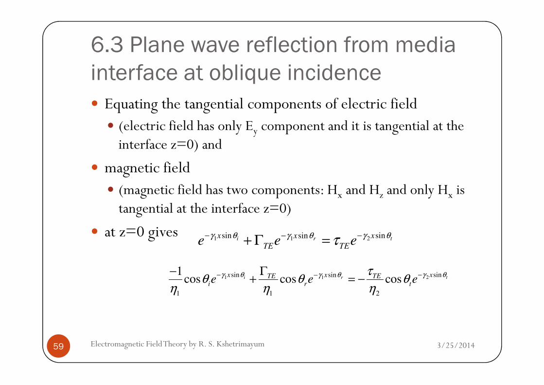
interface at oblique incidence
� Equating the tangential components of electric field � (electric field has only Ey component and it is tangential at the interface z=0) and
� magnetic field � (magnetic field has two components: Hx and Hz and only Hx is
3/25/2014Electromagnetic Field Theory by R. S. Kshetrimayum59
� (magnetic field has two components: Hx and Hz and only Hx is tangential at the interface z=0)
� at z=0 gives1 21sin sinsini trx xx
TE TEe e e
γ θ γ θγ θ τ− −−+ Γ =
1 21sin sinsin
1 1 2
1cos cos cosi trx xxTE TE
i r te e e
γ θ γ θγ θ τθ θ θ
η η η− −−Γ−
+ = −
6.3 Plane wave reflection from media
interface at oblique incidence
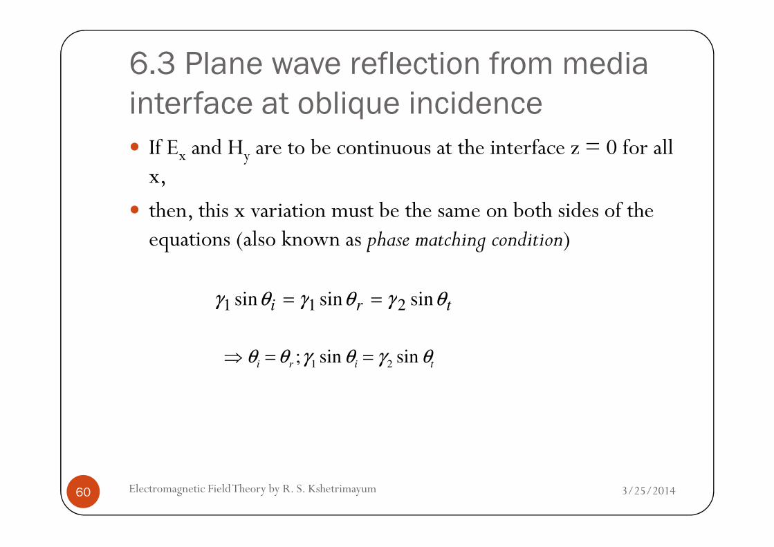
� If Ex and Hy are to be continuous at the interface z = 0 for all x,
� then, this x variation must be the same on both sides of the equations (also known as phase matching condition)
3/25/2014Electromagnetic Field Theory by R. S. Kshetrimayum60
tri θγθγθγ sinsinsin 211 ==
1 2; sin sin
i r i tθ θ γ θ γ θ⇒ = =

6.3 Plane wave reflection from media
interface at oblique incidence
� The first is Snell’s law of reflection � which states that the angle of incidence equals the angle of reflection
� The second result is the Snell’s law of refraction � (refraction is the change in direction of a wave due to change in
3/25/2014Electromagnetic Field Theory by R. S. Kshetrimayum61
� (refraction is the change in direction of a wave due to change in velocity from one medium to another medium)
� Also note that refractive index of a medium is defined as
0 0
0 0
r r
r r
p
cn
v
µ ε µ εµ ε
µ ε= = =

6.3 Plane wave reflection from media
interface at oblique incidence
� hence, for a lossless dielectric media,
Now we can simplify above two equations by applying Snell’s
2 2 22 2 1 2
1 1 2 11 1 1
sin
sin
i
t
v n
v n
µ ε εθ γ β
θ γ β µ ε ε= = = = = =
3/25/2014Electromagnetic Field Theory by R. S. Kshetrimayum62
� Now we can simplify above two equations by applying Snell’s two laws as follows
1TE TE
τ+ Γ =
1 1 2
cos coscosi r TE
TE t
θ θ τθ
η η η− + Γ = −
6.3 Plane wave reflection from media
interface at oblique incidence
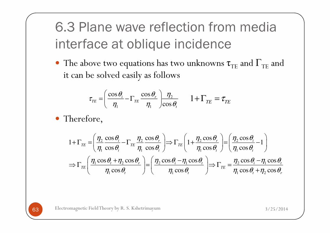
� The above two equations has two unknowns τTE and ГTE and it can be solved easily as follows
� Therefore,
2
1 1
cos cos
cos
i r
TE TE
t
θ θ ητ
η η θ
= − Γ
1TE TE
τ+ Γ =
3/25/2014Electromagnetic Field Theory by R. S. Kshetrimayum63
� Therefore,
22 2 2
1 1 1 1
1 2 2 1 2 1
1 1 1 2
cos coscos cos1 1 1
cos cos cos cos
cos cos cos cos cos cos
cos cos cos cos
i ir r
TE TE TE
t t t t
t r i t i t
TE TE
t t t r
θ η θη η θ η θ
η θ η θ η θ η θ
η θ η θ η θ η θ η θ η θ
η θ η θ η θ η θ
+ Γ = − Γ ⇒ Γ + = −
+ − −⇒Γ = ⇒Γ =
+

6.3 Plane wave reflection from media
interface at oblique incidence
� Hence, the reflection and transmission coefficients for oblique incidence (Fresnel coefficients) for perpendicular
2 1 1 2 2 1 2
1 2 1 2 1 2
cos cos cos cos cos cos 2 cos1 1
cos cos cos cos cos cos
i t t r i t i
TE TE
t r t r t r
η θ η θ η θ η θ η θ η θ η θτ
η θ η θ η θ η θ η θ η θ
− + + −∴ = + Γ = + = =
+ + +
3/25/2014Electromagnetic Field Theory by R. S. Kshetrimayum64
oblique incidence (Fresnel coefficients) for perpendicular polarization are given as follows:
� For normal incidence, it is a particular case and put
2 1
2 1
cos cos
cos cos
i t
TE
i t
η θ η θ
η θ η θ
−Γ =
+2
2 1
2 cos
cos cos
i
TE
i t
η θτ
η θ η θ=
+
0=== tri θθθ

6.3 Plane wave reflection from media
interface at oblique incidence
6.3.2 Parallel Polarization (TM):
� In this case, electric field vector lies in the xz plane� Since the magnetic field is transversal to the plane of incidence such waves are also called as transverse magnetic (TM) waves
3/25/2014Electromagnetic Field Theory by R. S. Kshetrimayum65
(TM) waves� So let us start with H vector which will have only y component,
( )ii xzi e
EyH
θθγ
ηsincos
1
0 1ˆ +−=r
6.3 Plane wave reflection from media
interface at oblique incidence
1
1
i
i
HH j E E
jωε
ωε
∇×∇× = ⇒ =
rr r r
Q
( ) ( )1 1cos sin cos sin
ˆ ˆ ˆ
1 i i i iz x z x
x y z
E e eγ θ θ γ θ θ− + − + ∂ ∂ ∂ ∂ ∂
3/25/2014Electromagnetic Field Theory by R. S. Kshetrimayum66
( )
( ) ( )
( ) { } ( )
1 1
1
1 1
cos sin cos sin
0
1 1 1
cos sin0
1
cos sin cos sin0 1
0
1 1
1ˆ ˆ
0 0
ˆ ˆˆ ˆcos sin cos si
i i i i
i i
i i i i
z x z x
z x
z x z x
i i i
E e ex z
j x y z j z x
Ee
Ee x z E e x z
j
γ θ θ γ θ θ
γ θ θ
γ θ θ γ θ θ
ωε ωε η
η
γθ θ θ
ωε η
− + − +
− +
− + − +
∂ ∂ ∂ ∂ ∂ = = − + ∂ ∂ ∂ ∂ ∂
= − = −( )ni
θ
6.3 Plane wave reflection from media
interface at oblique incidence
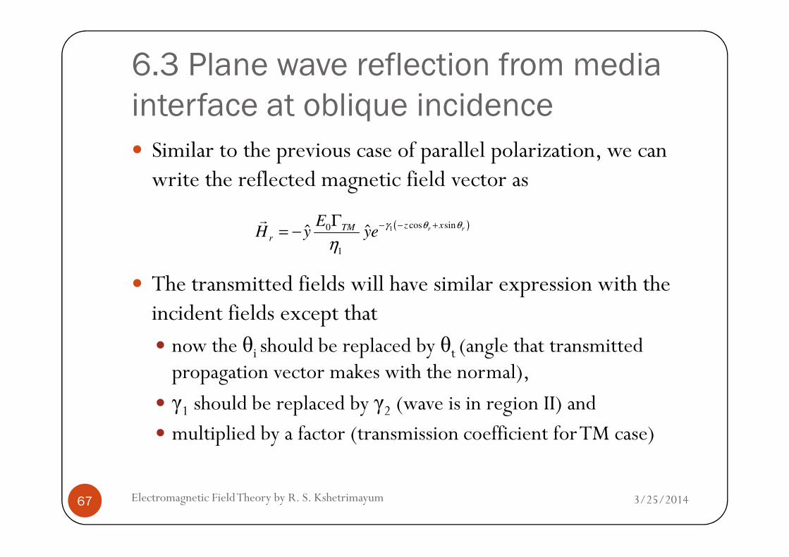
� Similar to the previous case of parallel polarization, we can write the reflected magnetic field vector as
� The transmitted fields will have similar expression with the
( )1 cos sin0
1
ˆ ˆ r rz xTM
r
EH y ye
γ θ θ
η
− − +Γ= −
r
3/25/2014Electromagnetic Field Theory by R. S. Kshetrimayum67
� The transmitted fields will have similar expression with the incident fields except that � now the θi should be replaced by θt (angle that transmitted propagation vector makes with the normal),
� γ1 should be replaced by γ2 (wave is in region II) and � multiplied by a factor (transmission coefficient for TM case)
6.3 Plane wave reflection from media
interface at oblique incidence
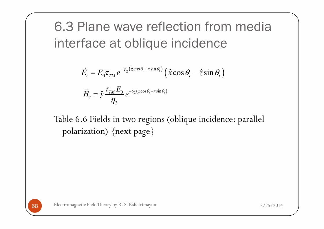
Table 6.6 Fields in two regions (oblique incidence: parallel
( ) ( )2cos sin
0ˆ ˆcos sint tz x
t TM t tE E e x z
γ θ θτ θ θ
− += −
r
( )2 cos sin0
2
ˆ t tz xTM
t
EH y e
γ θ θτ
η
− +=
r
3/25/2014Electromagnetic Field Theory by R. S. Kshetrimayum68
Table 6.6 Fields in two regions (oblique incidence: parallel polarization) {next page}

6.3 Plane wave reflection from media
interface at oblique incidence
Region I (lossy medium 1) Region II (lossy medium 2)
( ) ( )1 cos sin
0ˆ ˆcos sini iz x
i i iE E e x z
γ θ θ θ θ− += −
r
( )Er
( ) ( )2cos sin
0ˆ ˆcos sint tz x
t TM t tE E e x z
γ θ θτ θ θ
− += −
r
3/25/2014Electromagnetic Field Theory by R. S. Kshetrimayum69
( )ii xzi e
EyH
θθγ
ηsincos
1
0 1ˆ +−=r
( ) { }1 cos sin
0ˆ ˆcos sinr rz x
r TM r iE E e x z
γ θ θ θ θ− − += Γ +
r
( )1 cos sin0
1
ˆ ˆ r rz xTM
r
EH y ye
γ θ θ
η
− − +Γ= −
r
( )2 cos sin0
2
ˆ t tz xTM
t
EH y e
γ θ θτ
η− +
=r
6.3 Plane wave reflection from media
interface at oblique incidence
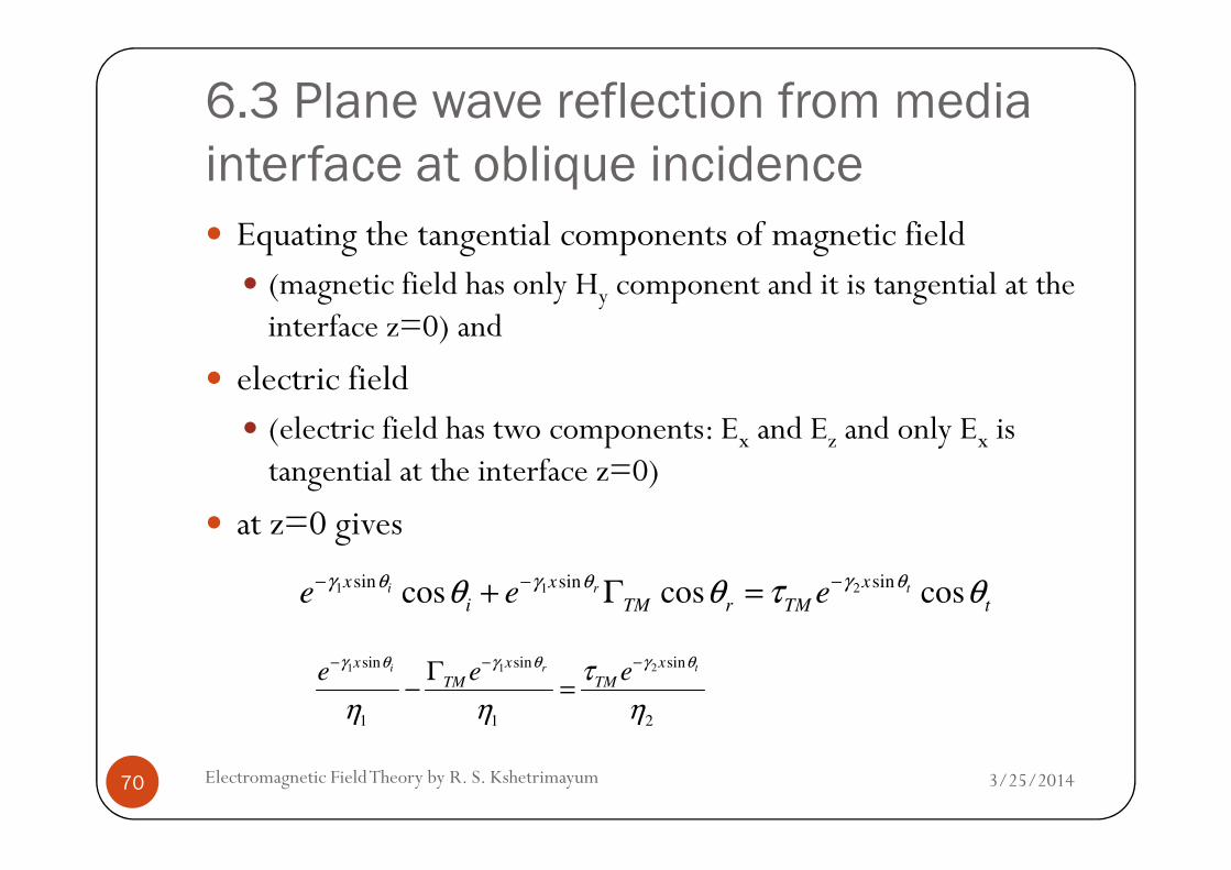
� Equating the tangential components of magnetic field � (magnetic field has only Hy component and it is tangential at the interface z=0) and
� electric field � (electric field has two components: Ex and Ez and only Ex is
3/25/2014Electromagnetic Field Theory by R. S. Kshetrimayum70
� (electric field has two components: Ex and Ez and only Ex is tangential at the interface z=0)
� at z=0 gives
1 21sin sinsincos cos cosi trx xx
i TM r TM te e e
γ θ γ θγ θθ θ τ θ− −−+ Γ =
21 1 sinsin sin
1 1 2
ti r xx x
TM TMe ee
γ θγ θ γ θ τ
η η η
−− −Γ− =
6.3 Plane wave reflection from media
interface at oblique incidence
� Therefore,
which is Snell’s law of reflection and refraction and this
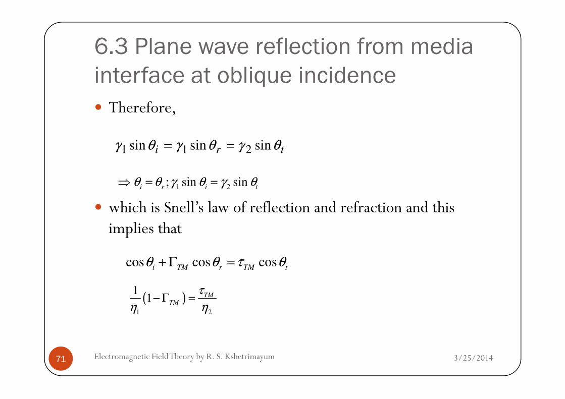
tri θγθγθγ sinsinsin 211 ==
1 2; sin sin
i r i tθ θ γ θ γ θ⇒ = =
3/25/2014Electromagnetic Field Theory by R. S. Kshetrimayum71
� which is Snell’s law of reflection and refraction and this implies that
cos cos cosi TM r TM t
θ θ τ θ+ Γ =
( )1 2
11 TM
TM
τ
η η− Γ =
6.3 Plane wave reflection from media
interface at oblique incidence
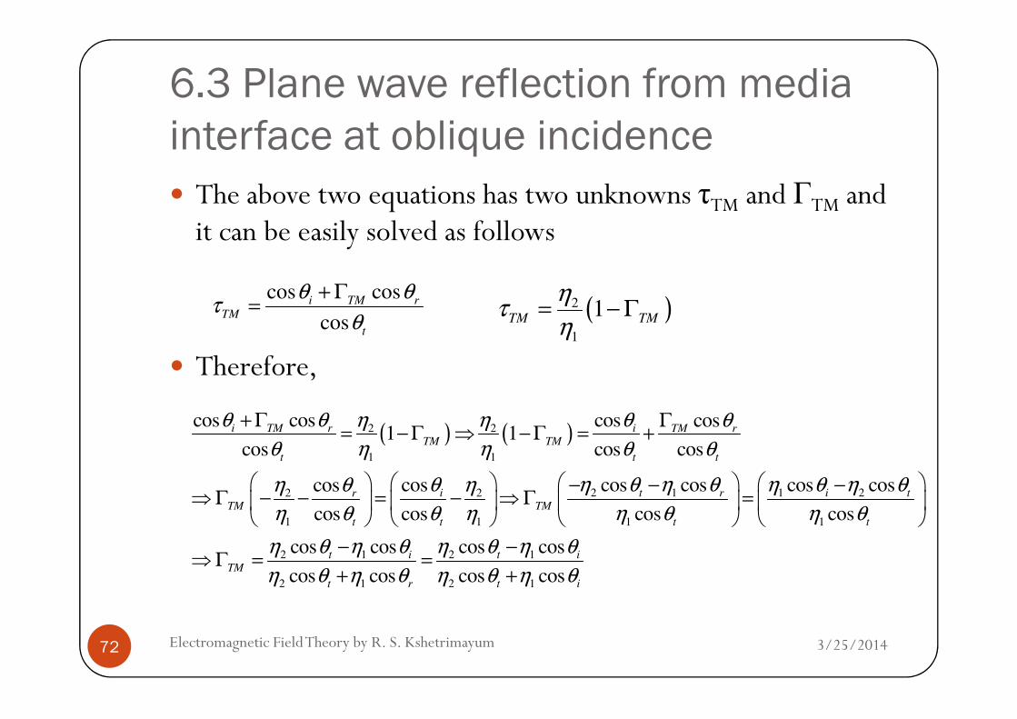
� The above two equations has two unknowns τTM and ГTM and it can be easily solved as follows
� Therefore,
cos cos
cos
i TM r
TM
t
θ θτ
θ
+ Γ= ( )2
1
1TM TM
ητ
η= − Γ
3/25/2014Electromagnetic Field Theory by R. S. Kshetrimayum72
� Therefore,
( ) ( )2 2
1 1
2 1 1 22 2
1 1 1 1
2 1
2
cos cos cos cos1 1
cos cos cos
cos cos cos cos coscos
cos cos cos cos
cos cos
cos
i TM r i TM r
TM TM
t t t
i t r i tr
TM TM
t t t t
t i
TM
θ θ θη η θ
θ η η θ θ
θ η θ η θ η θ η θη θ η
η θ θ η η θ η θ
η θ η θ
η θ
+ Γ Γ= − Γ ⇒ − Γ = +
− − −⇒ Γ − − = − ⇒ Γ =
−⇒ Γ = 2 1
1 2 1
cos cos
cos cos cos
t i
t r t i
η θ η θ
η θ η θ η θ
−=
+ +
6.3 Plane wave reflection from media
interface at oblique incidence
� Hence, the reflection and transmission coefficients for oblique
( ) 2 1 2 1 2 12 2 2
1 1 2 1 1 2 1
1 22
1 2 1 2 1
cos cos cos cos cos cos1 1
cos cos cos cos
2 cos 2 cos
cos cos cos cos
t i t i t i
TM TM
t i t i
i i
t i t i
η θ η θ η θ η θ η θ η θη η ητ
η η η θ η θ η η θ η θ
η θ η θη
η η θ η θ η θ η θ
− + − +∴ = − Γ = − =
+ +
= =
+ +
3/25/2014Electromagnetic Field Theory by R. S. Kshetrimayum73
Hence, the reflection and transmission coefficients for oblique incidence (Fresnel coefficients) for parallel polarization are given as follows:
� Note that cosine terms multiplication in the above equations is different from the previous expression for TE waves
2 1
2 1
cos cos
cos cos
t i
TM
t i
η θ η θ
η θ η θ
−∴Γ =
+
2
2 1
2 cos
cos cos
i
TM
t i
η θτ
η θ η θ=
+
6.3 Plane wave reflection from media
interface at oblique incidence
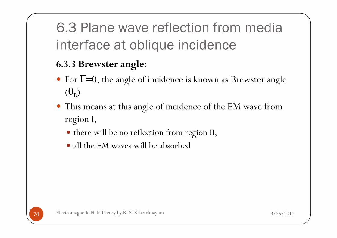
6.3.3 Brewster angle:
� For Γ=0, the angle of incidence is known as Brewster angle (θB)
� This means at this angle of incidence of the EM wave from region I,
3/25/2014Electromagnetic Field Theory by R. S. Kshetrimayum74
region I, � there will be no reflection from region II, � all the EM waves will be absorbed
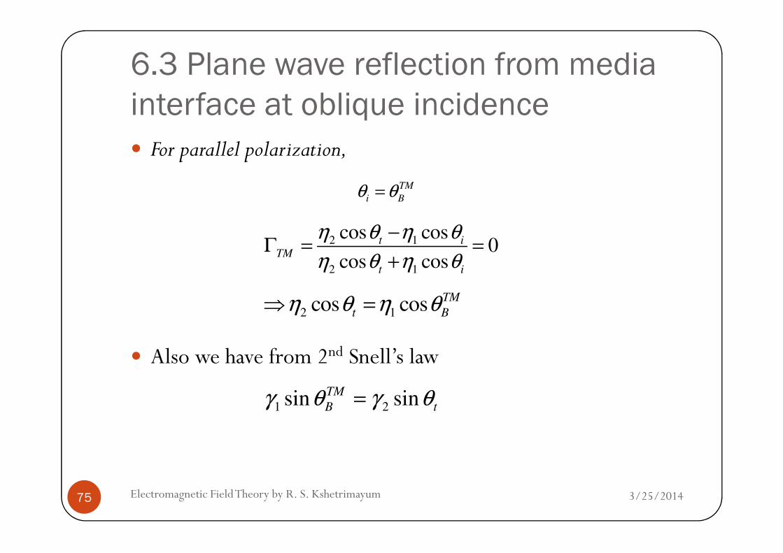
6.3 Plane wave reflection from media
interface at oblique incidence
� For parallel polarization,
2 1
2 1
cos cos0
cos cos
t i
TM
t i
η θ η θ
η θ η θ
−Γ = =
+
TM
i Bθ θ=
3/25/2014Electromagnetic Field Theory by R. S. Kshetrimayum75
� Also we have from 2nd Snell’s law
2 1cos cos
TM
t Bη θ η θ⇒ =
t
TM
B θγθγ sinsin 21 =
6.3 Plane wave reflection from media
interface at oblique incidence
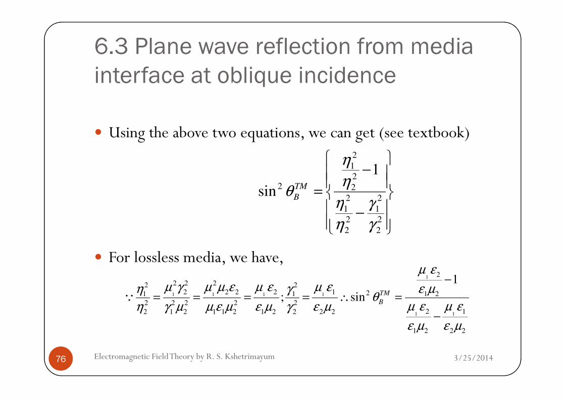
� Using the above two equations, we can get (see textbook)
−
=22
2
2
2
1
2
1
sinγη
η
η
θ TM
B
3/25/2014Electromagnetic Field Theory by R. S. Kshetrimayum76
� For lossless media, we have,1
1 1 1 1
1 1
2
2 2 22 22 2 2 2 1 21 1 1 2
2 2 2 2 2
2 12 1 2 1 1 2 1 2 2 2 2
1 2 2 2
1
; sinTM
B
µ ε
µ γ µ µ ε µ ε µ εη γ ε µθ
µ ε µ εη γ µ µ ε µ ε µ γ ε µ
ε µ ε µ
−
= = = = ∴ =
−
Q
−
2
2
2
1
2
2
2
1
γ
γ
η
ηB
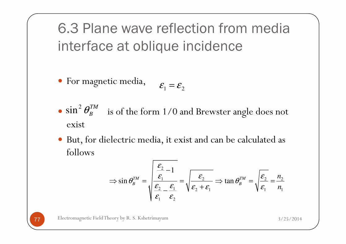
6.3 Plane wave reflection from media
interface at oblique incidence
� For magnetic media,
� is of the form 1/0 and Brewster angle does not exist
21εε =
TM
Bθ2sin
3/25/2014Electromagnetic Field Theory by R. S. Kshetrimayum77
exist� But, for dielectric media, it exist and can be calculated as follows
2
1 2 2 2
2 1 2 1 1 1
1 2
1
sin tanTM TM
B B
n
n
ε
ε ε εθ θ
ε ε ε ε εε ε
−
⇒ = = ⇒ = =+−
6.3 Plane wave reflection from media
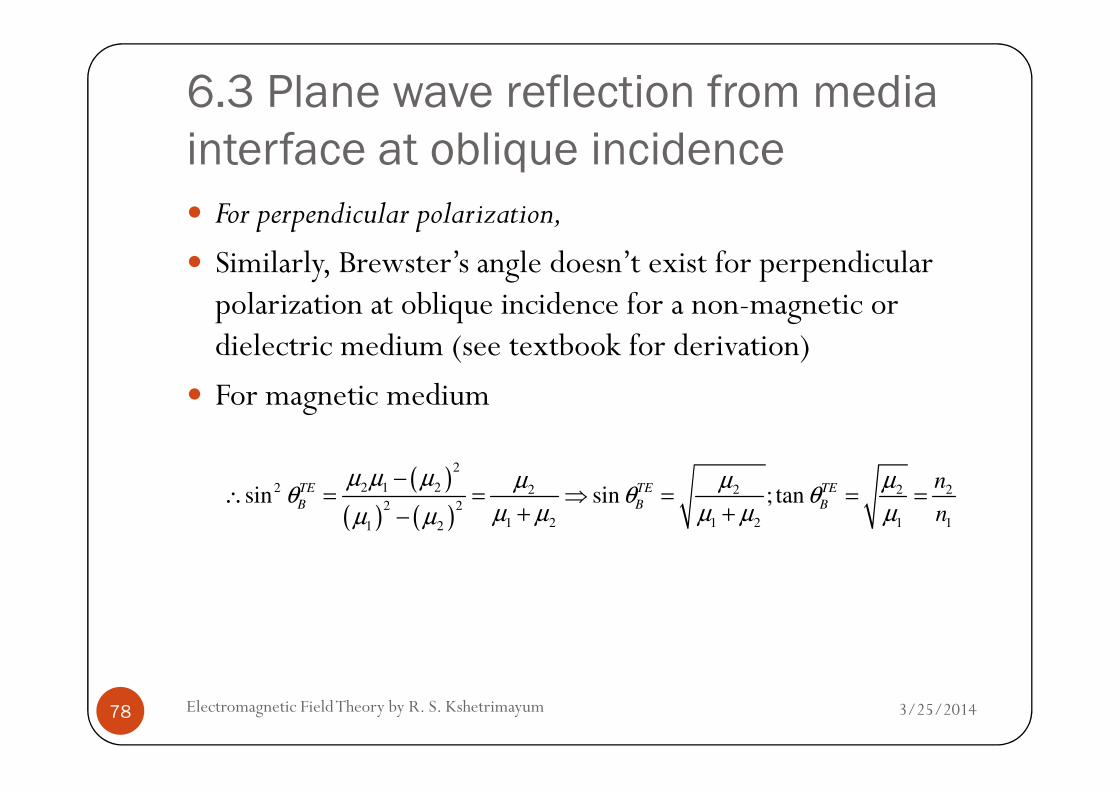
interface at oblique incidence
� For perpendicular polarization,
� Similarly, Brewster’s angle doesn’t exist for perpendicular polarization at oblique incidence for a non-magnetic or dielectric medium (see textbook for derivation)
� For magnetic medium
3/25/2014Electromagnetic Field Theory by R. S. Kshetrimayum78
� For magnetic medium
( )
( ) ( )
2
2 1 22 2 2 2 2
2 2
1 2 1 2 1 11 2
sin sin ; tanTE TE TE
B B B
n
n
µ µ µ µ µ µθ θ θ
µ µ µ µ µµ µ
−∴ = = ⇒ = = =
+ +−
6.3 Plane wave reflection from media
interface at oblique incidence� Brewster angle exist for oblique incidence (perpendicular polarization) for interface between two magnetic media
� An incident wave consisting of both polarizations will have reflected wave for only one polarization for Brewster angle
� Brewster angle is also known as Polarizing angle (used in optics and lasers)
3/25/2014Electromagnetic Field Theory by R. S. Kshetrimayum79
Polarizing angle optics and lasers)
� In other words, an incident wave which is composed of both TE and TM waves will have reflected TE (TM) waves only for dielectric (magnetic) media interface
� Thus, a circularly polarized incident wave at polarizing angle will become a linearly polarized wave
6.3 Plane wave reflection from media
interface at oblique incidence
6.3.4 Total internal reflection:
� Used in optical fibers� Light strikes an angle of incidence greater than critical angle,
� all of the light energy will be reflected back, and � none of them will be absorbed
3/25/2014Electromagnetic Field Theory by R. S. Kshetrimayum80
� none of them will be absorbed
� This critical angle is related to the refractive index of the two media and is given by
� where are the refractive index of medium 2 and 1 respectively
1 2
1
sinc
n
nθ −
=
6.3 Plane wave reflection from media
interface at oblique incidence
� In fact, this can be observed for both the polarizations we have discussed above
� From Snell’s Second law, we have,
2
1 2
sinsin sin sin t
i t i
γ θγ θ γ θ θ
γ= ⇒ =
3/25/2014Electromagnetic Field Theory by R. S. Kshetrimayum81
� If we consider non-magnetic materials (dielectrics) of , in that case,
1 2
1
sin sin sini t i
γ θ γ θ θγ
= ⇒ =
2
1
sinsin
t
i
ε θθ
ε⇒ =

6.3 Plane wave reflection from media
interface at oblique incidence
� Hence, for
� (it means the transmitted wave travels along the interface, for our case, it is x-axis) which implies that
,2
i c t
πθ θ θ= =
3/25/2014Electromagnetic Field Theory by R. S. Kshetrimayum82
our case, it is x-axis) which implies that
2 1 2
11
sin sinc c
ε εθ θ
εε
−
⇒ = ⇒ =

6.3 Plane wave reflection from media
interface at oblique incidence
� We can write the above relation as
Note that to have a real value of critical angle
1 1 1 10 2 0 22 2 2 2
1 0 1 0 1 1 1 1
sin sin sin sinr r r r
c
r r r r
n
n
µ µ ε εε µ εθ
ε µ µ ε ε µ ε− − − −
= = = =
ε ε>
3/25/2014Electromagnetic Field Theory by R. S. Kshetrimayum83
� Note that to have a real value of critical angle� Besides, we have assumed that for a dielectric,
1 2ε ε>
1 21
r rµ µ= =
6.3 Plane wave reflection from media
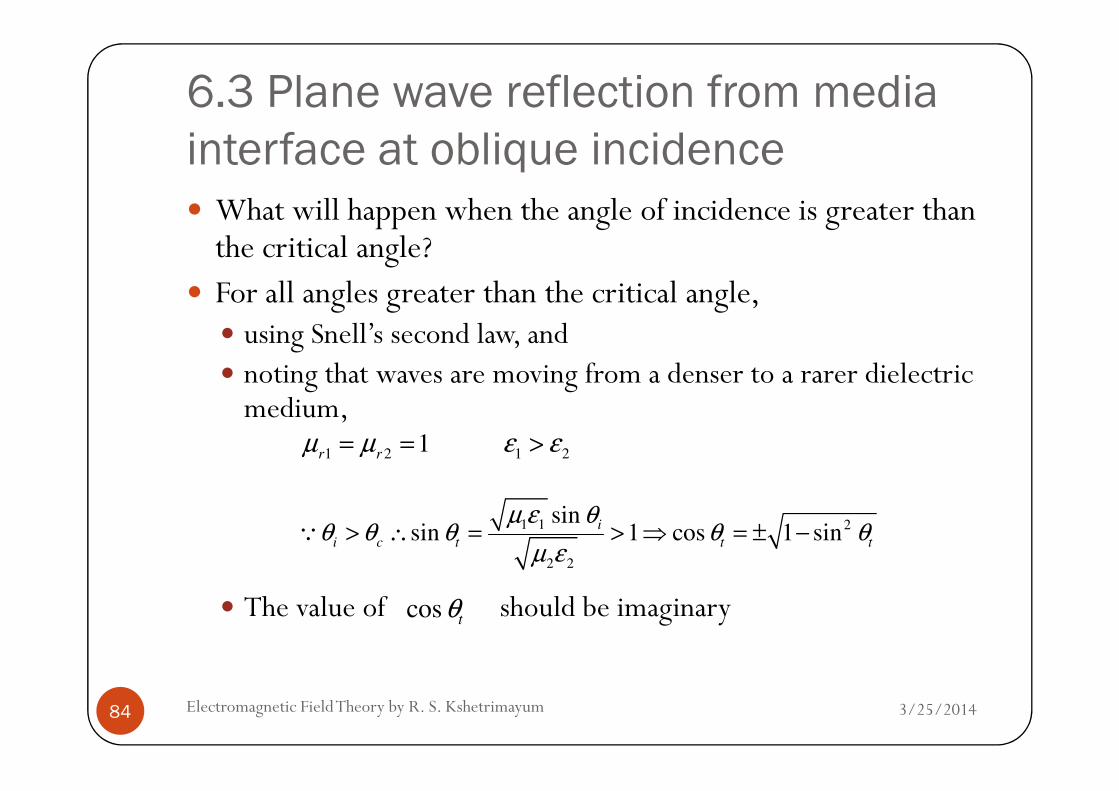
interface at oblique incidence� What will happen when the angle of incidence is greater than the critical angle?
� For all angles greater than the critical angle, � using Snell’s second law, and � noting that waves are moving from a denser to a rarer dielectric medium,
3/25/2014Electromagnetic Field Theory by R. S. Kshetrimayum84
medium,
� The value of should be imaginary
1 1 2
2 2
sinsin 1 cos 1 sin
i
i c t t t
µ ε θθ θ θ θ θ
µ ε> ∴ = > ⇒ = ± −Q
cost
θ
1 21
r rµ µ= =
1 2ε ε>

6.3 Plane wave reflection from media
interface at oblique incidence
� It can be shown that (see textbook for derivation)
� For z>0, since is an imaginary number, is also purely imaginary
2 2
2 2
0 02 cos 2 cos* *
2 2
ˆ ˆsin cost tj z j z
t t
E ES E H x e z e
β θ β θτ τθ θ
η η− −∴ = × = +
r r r
cost
θ *cos
tθ
3/25/2014Electromagnetic Field Theory by R. S. Kshetrimayum85
also purely imaginary� Hence, the second term is imaginary, therefore, no real power is flowing along z-axis in region II
� The first term which has direction along x-axis is real and is exponentially decaying with z
6.3 Plane wave reflection from media
interface at oblique incidence
� Hence,� When a wave is incident at an angle of incidence greater than or equal to the critical angle from region I,
� the wave will be total internally reflected in region I� Surface waves exist in the region II,
3/25/2014Electromagnetic Field Theory by R. S. Kshetrimayum86
� Surface waves exist in the region II, � which is propagating along x-axis (direction of power flow), and
� attenuating very fast along z-axis � People have used this for communications using submarines
6.3 Plane wave reflection from media
interface at oblique incidence
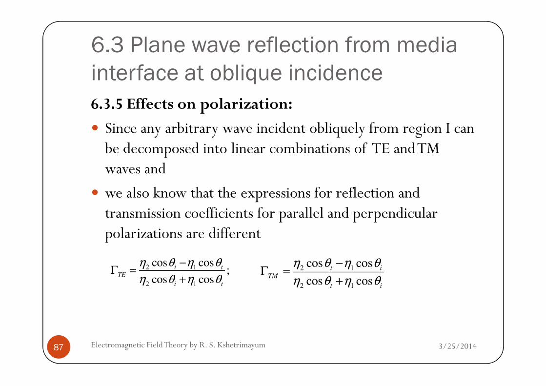
6.3.5 Effects on polarization:
� Since any arbitrary wave incident obliquely from region I can be decomposed into linear combinations of TE and TM waves and
� we also know that the expressions for reflection and
3/25/2014Electromagnetic Field Theory by R. S. Kshetrimayum87
� we also know that the expressions for reflection and transmission coefficients for parallel and perpendicular polarizations are different
2 1
2 1
cos cos;
cos cos
i t
TE
i t
η θ η θ
η θ η θ
−Γ =
+2 1
2 1
cos cos
cos cos
t i
TM
t i
η θ η θ
η θ η θ
−Γ =
+
6.3 Plane wave reflection from media
interface at oblique incidence
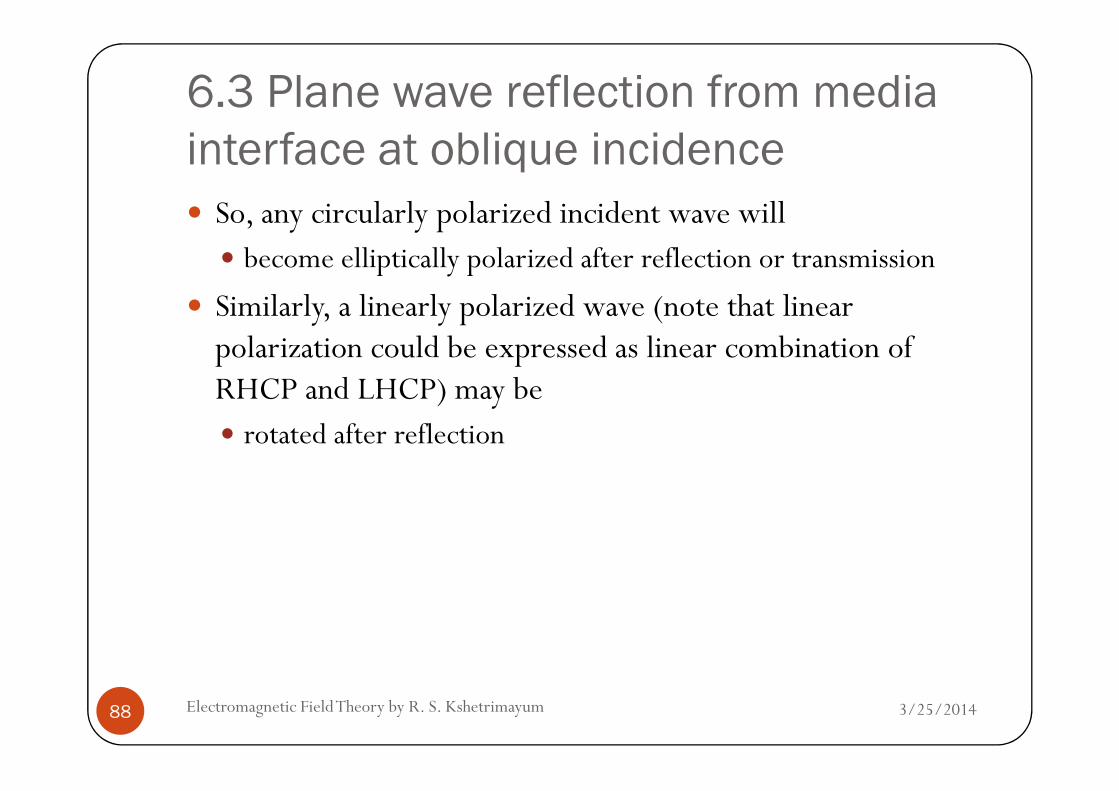
� So, any circularly polarized incident wave will � become elliptically polarized after reflection or transmission
� Similarly, a linearly polarized wave (note that linear polarization could be expressed as linear combination of RHCP and LHCP) may be
3/25/2014Electromagnetic Field Theory by R. S. Kshetrimayum88
RHCP and LHCP) may be � rotated after reflection

6.3 Plane wave reflection from media
interface at oblique incidence
� For instance, � If the region II is a perfect conductor, η2=0, Г=-1 for both TE and TM cases, � this means a RHCP wave after reflection will become LHCP
3/25/2014Electromagnetic Field Theory by R. S. Kshetrimayum89
� this means a RHCP wave after reflection will become LHCP wave and vice versa
� This is why circular polarization is not used for indoor communication systems since we have many reflections inside a room
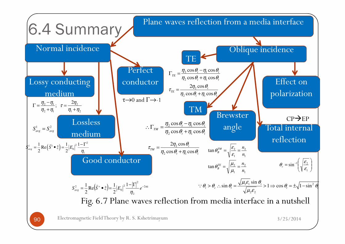
6.4 SummaryPlane waves reflection from a media interface
Normal incidenceTE
Lossless
Oblique incidence
Lossy conducting medium
Perfect conductor
TM Brewster angle
Effect on polarization
2 1
2 1
;η η
η η
−Γ =
+2
1 2
2ητ
η η=
+
τ→0 and Γ→-1
2 1
2 1
cos cos
cos cos
i t
TE
i t
η θ η θ
η θ η θ
−Γ =
+
2
2 1
2 cos
cos cos
i
TE
i t
η θτ
η θ η θ=
+
cos cosη θ η θ−CP�EP
3/25/2014Electromagnetic Field Theory by R. S. Kshetrimayum90
Lossless medium
Good conductor
Fig. 6.7 Plane waves reflection from media interface in a nutshell
angle Total internal reflection
( )2
21 1
0
1
1 1 1ˆRe
2 2avg
S S z Eη
− Γ= • =
r
1 2
avg avgS S=
2 1
2 1
cos cos
cos cos
t i
TM
t i
η θ η θ
η θ η θ
−∴Γ =
+
2
2 1
2 cos
cos cos
i
TM
t i
η θτ
η θ η θ=
+
CP�EP
= −
1
21sin
ε
εθc
1
2
1
2tann
nTM
B ==ε
εθ
1
2
1
2tann
nTE
B ==µ
µθ
1 1 2
2 2
sinsin 1 cos 1 sin
i
i c t t t
µ ε θθ θ θ θ θ
µ ε> ∴ = > ⇒ = ± −Q( ) z
avg eEzSSα
η2
2
2
2
0
21
2
1ˆRe
2
1 −+ Γ−=•=
r