Finance and Economics Discussion SeriesDivisions of Research & Statistics and Monetary Affairs

Federal Reserve Board, Washington, D.C.

Interconnectedness in the Interbank Market

Celso Brunetti, Jeffrey H. Harris, Shawn Mankad, and GeorgeMichailidis

2015-090

Please cite this paper as:Brunetti, Celso, Jeffrey H. Harris, Shawn Mankad, and George Michailidis (2015).“Interconnectedness in the Interbank Market,” Finance and Economics Discussion Se-ries 2015-090. Washington: Board of Governors of the Federal Reserve System,http://dx.doi.org/10.17016/FEDS.2015.090.

NOTE: Staff working papers in the Finance and Economics Discussion Series (FEDS) are preliminarymaterials circulated to stimulate discussion and critical comment. The analysis and conclusions set forthare those of the authors and do not indicate concurrence by other members of the research staff or theBoard of Governors. References in publications to the Finance and Economics Discussion Series (other thanacknowledgement) should be cleared with the author(s) to protect the tentative character of these papers.

Interconnectedness in the Interbank Market

Celso Brunetti, Jeffrey H. Harris, Shawn Mankad, George Michailidis Abstract: We study the behavior of the interbank market before, during and after the 2008 financial crisis. Leveraging recent advances in network analysis, we study two network structures, a correlation network based on publicly traded bank returns, and a physical network based on interbank lending transactions. While the two networks behave similarly pre-crisis, during the crisis the correlation network shows an increase in interconnectedness while the physical network highlights a marked decrease in interconnectedness. Moreover, these networks respond differently to monetary and macroeconomic shocks. Physical networks forecast liquidity problems while correlation networks forecast financial crises. Acknowledgements: We would like to thank for valuable discussions and comments: Kirsten Anderson, Stefano Battiston, Guido Caldarelli, Rama Cont, Michael Gordy, Erik Heitfield, Andrew Karolyi, Luigi Ruggerone, and Clara Vega, and seminar participants at Babson College, Cornell University, Hull University, the CFTC and the Board of Governors, and participants to the conference of the Society for Computational Economics, Oslo, 2014, the International Association for Applied Econometrics Annual Conference, London, 2014, the workshop on “Systemic risk and macro‐prudential regulation: perspectives from network analysis,” Bank of England, 2014, and the conference on “Behavioral Aspects in Macroeconomics and Finance,” Milan 2014. A preliminary draft of this paper was titled “The Breakdown of the Interbank Market during the Financial Crisis.” All errors are ours. The views in this paper should not be interpreted as reflecting the views of the Board of Governors of the Federal Reserve System or of any other person associated with the Federal Reserve System. All errors and omissions, if any, are the authors’ sole responsibility Celso Brunetti (celso.brunetti@frb.gov) is in the Division of Research and Statistics at the Federal Reserve Board; Jeffrey H. Harris (jharris@american.edu) is at American University’s Kogod School of Business; Shawn Mankad (smankad@rhsmith.umd.edu) is at University of Maryland's Smith School of Business; George Michailidis (gmichail@umich.edu) is in the Department of Statistics at the University of Michigan.

1

1. Introduction

The breakdown of liquidity in normally robust financial markets presents one of the

enduring questions from the recent financial crisis. During the crisis, central bank

intervention failed to enhance liquidity, and over short intervals, crowded out private

liquidity (Brunetti, di Filippo and Harris (2011)). In addition, precautionary hoarding

by relatively weak banks during the crisis appeared to exacerbate market liquidity

problems as well.1 Given the central role that banks play in providing valuable

liquidity to many markets, the interbank market plays a significant role in

facilitating market liquidity.2

In this paper, we study interconnectedness in the European interbank market

to explore whether, and how, bank interconnectedness evolves during the crisis using

two different network structures—the correlation (Granger-causality) network of

bank stock returns (Billio et al. (2012)) and the physical interbank trading network.

We study how interconnectedness in these networks is affected by monetary and

macroeconomic shocks related to the European Central Bank (ECB) interventions

and announcements of both conventional and unconventional ECB operations (see

Rogers, Scotti and Wright (2014)). Further, we explore whether interconnectedness

metrics help to forecast financial and economic activity.

We show that during the crisis, physical network connectedness drops

significantly, reflecting hoarding behavior among banks which impairs interbank

1 See, for instance, Acharya, Shin, and Yorulmazer (2010), Heider, Hoerova, and Holthausen (2010, Ashcraft, McAndrews and Skeie (2011), Acharya and Skeie (2011), and Acharya and Merrouche (2012). 2 Interconnectedness is one of the five (equally-important) characteristics used by the European Union to determine globally systemic important banks, or G-SIBs (BIS (2011)).

2

market liquidity. Conversely, and similar to results in Billio et al. (2012), we find that

European bank correlation networks reveal increased connectedness during the

crisis. These network-based findings show that correlation and physical networks

evolve differently and reflect different economic content. While the physical trading

network reveals the breakdown between banks, the correlation network reveals that

banks equity returns were driven by a common factor during the crisis.

Moreover, we find that correlation and physical networks respond differently

to monetary and macroeconomic shocks. Early in the crisis central banks intervened

heavily to promote funding and market liquidity. Interconnectedness in physical

networks adjusts strongly and quickly to these central bank operations and

announcements, revealing important market characteristics related to interbank

trading at short (daily) horizons. Conversely, interconnectedness in correlation

networks changes little in response to these events, presumably since these

announcements and interventions have little impact on the common factor driving

stock returns. In this light, monitoring the response of the interbank market to

announcements and interventions is more valuable to policy makers interested in

enhancing interconnectedness among banks.

We further compare networks to test whether interconnectedness measures

might serve to forecast short-term economic conditions. We show that correlation

networks can identify (and forecast) periods of impending financial crises.

Complementarily, physical interbank trading networks serve to identify weakening

interconnectedness in the interbank system that may lead to liquidity problems.

3

From a policy perspective, understanding both types of networks can be useful.

Correlation networks constructed from equity market returns rely on publicly-traded

equity prices, and so cannot isolate problem banks which are privately held. Likewise,

correlation networks cannot distinguish between common exposures and contagion,

nor can they identify the different channels of contagion, a precondition for preventive

and palliative actions by policy makers and regulators. While correlation networks

might better identify systemic risk,3 physical networks respond to smaller exogenous

shocks and are useful in identifying both systemically important and problem banks

on an on-going basis. Physical networks are therefore more useful when exogenous

shocks are not large enough to threaten systemic risk (i.e. most of the time). Since

market liquidity depends crucially on the connectedness between banks, regulators

would be well suited to monitor the interbank market for early signs of liquidity

problems.

Our work contributes to the literature on networks in finance, which, broadly

speaking, distinguishes between correlation networks, where edges are based on

indirect links like return correlations (e.g. Diebold and Yilmaz (2014), Billio et al.

(2012)), and physical networks, where direct links result from agent choices (e.g.,

banks A and B contract to exchange overnight funds as in Cont, Moussa and Santos

(2012)). We develop an accounting framework that helps to illuminate the different

nature of the two network structures. We then utilize the direct nature of trade in

3 See Puliga, Caldarelli and Battiston (2014).

4

our data to compare and contrast correlation networks with physical networks in our

empirical work.

The paper proceeds as follows. In Section 2, we provide a review of the main

literature. In Section 3, we provide an accounting framework which helps

understanding the two different network formations. Section 4 describes our data,

while Section 5 describes the interconnectedness metrics from the correlation and

physical networks we construct. In Section 6, we study how central bank

announcements and interventions, and traditional financial variables affect network

topology in a forecasting exercise. We conclude with a brief discussion in Section 7.

2. Network Interconnectedness Literature

A number of research papers highlight how common holdings can drive

interconnectedness within correlation networks. Much of the literature on networks

in finance concentrates on how network structures are important for the propagation

of shocks. Allen and Gale’s (2000) seminal paper shows that the network structure

may exacerbate or attenuate contagion effects.4 In this literature, linkages

(interconnectedness) between financial institutions may occur either as a result of

common holdings or as a result of direct contractual agreements.

Braverman and Minca (2014) describe how common asset holdings among

banks can transmit financial distress. If two banks, A and B, hold the same asset in

their portfolios and an exogenous shock forces A to liquidate the asset, the price of

4 See also Upper (2006).

5

the asset will decline and therefore change the value of B’s portfolio. In this way,

common asset holdings generate networks that transmit shocks between (and among)

banks. While links in the network of common asset holdings are not readily specified

in bank balance sheets, they may be estimated by stock market price linkages.

In line with equity market reactions, Braverman and Minca (2014) show that

the severity of contagion depends on both common holdings and the liquidity of these

common holdings. In their network model, the higher the number of common assets

in the portfolios the higher is the possibility of contagion (a point first introduced by

Shaffer (1994)). In a similar vein, Lagunoff and Schreft (1998) develop a game-

theoretic model which shows that as economies increase in size, diversification

opportunities also increase which, in turn, reduces network fragility. However, if the

increase exceeds a given threshold, the high level of interconnectedness may increase

financial fragility.

Indeed, Cont and Wagalath (2011) show that realized correlations in equity

indices increased dramatically with the collapse of Lehman Brothers on September

15, 2008. They conjecture that the increased correlation resulted from the liquidation

of large positions by market participants (fire sales) and develop a model in which

returns are driven by both fundamentals and liquidity. They highlight the limits of

diversification—even in the absence of correlation between fundamentals, liquidity

correlations among large assets can generate correlated asset returns, “thus losing

the benefit of diversification exactly when it is needed.” (p.4).

6

Cabrales and Gottardi (2014) model contagion as the transmission of a

pathologic disease, linking firms as they exchange assets to meet capital

requirements. They note that there is a trade-off between risk-sharing and contagion

among firms. Similarly, De Vries (2005) claims that banks, by holding similar

portfolios, are exposed to the same market risks so that bank equity returns are

asymptotically dependent. Likewise, Acharya and Yorulmazer (2008) show that if

banks hold stakes in the same companies (e.g. for diversification purposes) bank

equities are necessarily interdependent.

A second burgeoning literature on financial networks examines contractual

agreements similar to our physical network constructed from interbank trades. For

example, Acemoglu, Ozdaglar and Tahbaz-Salehi (2013) find that financial contagion

is a function of the network structure. They confirm (as in Allen and Gale (2000))

that a network where all banks are connected is less fragile than an incomplete

network for small exogenous shocks. However, for large shocks, a more

interconnected network facilitates contagion, creating a more fragile system.

Similarly, Gai, Haldane and Kapadia (2011) present a theoretical framework to

identify tipping points in complex systems, whereby small shocks can have large

consequences.

Some works consider both correlation and physical networks. Cifuentes,

Ferrucci and Shin (2005) construct a model that incorporates two channels of

contagion: direct linkages through the interbank market and indirect linkages

through common holdings. Similarly, Caccioli, Farmer, Foti and Rockmore (2013)

7

analyze both the network of common holdings and the physical network and show

that in a crisis, contagion is mainly driven by common holdings but it is amplified by

trading the physical network—i.e. both networks contribute to systemic risk.5

Most of this literature highlights the fact that common asset holdings, reflected

in correlation networks, are the main source of systemic risk (Elsinger, Lehar and

Summer (2006)) and that interbank lending (the physical network of bank

connections) plays only a marginal role. Conversely, we analyze these networks from

a different angle. We aim to quantify the information content of these two network

structures to better understand how policy decisions might be more effective in

ameliorating systemic risk and enhancing market liquidity in times of crisis.

3. An Accounting Framework

In order to highlight the two different network formations, we adopt a simple

accounting framework (following Shin (2009a, 2009b) and Elliott, Golub and Jackson

(2014)). We consider a simple financial system in which banks connect lenders to

borrowers as intermediaries, collecting deposits from households and firms and

investing the deposits in a portfolio of assets, including loans to the household sector

(via mortgages and consumer debt) and firms.

We introduce now some notation:

5 See also Allen and Babus (2010) and Allen, Babus and Carletti (2010). In related work, Roukny, Bersini, Pirotte, Caldarelli and Battiston (2013) analyze bank network topology and find that topology matters only when the market is illiquid.

8

1. , denotes the market value of bank i’s assets—including loans to firms and

households as well as k asset classes (equities, bonds, commodities, etc.).

2. , is the weight invested in each of the k assets by bank i; ∑ , 1 ;

3. denotes the total value of liabilities of bank i held by other banks;

4. , is the value of bank i’s liabilities held by bank j;

5. , is the share of bank i’s liabilities held by bank j;

6. indicates the market value of bank i’s equity;

7. is the total value of liabilities of bank i held by non-banks.

Hence, banks i’s balance sheet is given by

Assets Liabilities

, ,

(1)

,

and bank i’s balance sheet identity is

, , , 2

9

The left hand side is the value of all bank i’s assets which is equal to the market

value of bank i’s portfolio, first term, and to the funds lent by bank i to other banks

(interbank lending), second term.6

From equation (2) we can express the vector of interbank debt as follows

3

and

4

The left hand side is the interbank market which, according to (4), depends on the

market value of the portfolio of assets held by banks, the market value of bank

equities and the value of bank liabilities held by non-banks. The interbank market is

dynamic, with daily trading (overnight loans represent the overwhelming majority—

92.3%—of contracts in e-MID) in response to their funding needs (commonly linked to

minimum reserve requirements, margin calls, or shortages needed to fulfill

contractual obligations, represented by the first term of the right hand side of (4)).

Bank equity (E) changes over time may also drive interbank lending through the

second term on the right hand side of (4).

Following Shin (2009a), we assume that the debt liabilities to non-banks are

expected to be sticky—i.e. D is will move very slowly. D represents debt claims on the

banking sector by households, mutual and pension funds and other non-bank

institutions, so while D varies over time, changes to D are less likely to drive

interbank lending.

6 We assume that banks have restrictions for cross holdings of equities. This assumption can be easily relaxed in our model.

10

Given the accounting identity that governs the full system of banks, we

represent the adjacency matrix of the interbank lending market as follows.

Bank 1 Bank 2 … Bank s

Bank 1 0 , … ,

Bank 2 , 0 … ,

… … …

Bank s , , … 0

From equation (4) we build the consolidated balance sheet of the banking

sector as whole where assets and liabilities are aggregated across banks. Given that

, is a liability for bank i but an asset for bank j, the aggregated balance sheet does

not include any interbank claims. Hence, (1) becomes

Assets Liabilities

, ,

(5)

and the balance sheet identity is now7

6

7 Equation (6) has an interpretation similar to that in Elliott et al. (2014) and is based on the results in Brioschi, Buzzacchi and Colombo (1989) and Fedenia, Hodder and Triantis (1994). De Vries (2005) offers an interesting interpretation of (6): “The fortunes of the banking sector as indicated by the balance sheet items, are sooner or later also reflected in the value of bank equity. This enables us to characterize systemic failure in terms of the joint bank equity price movements, which are driven by the interdependent bank portfolios.” (p.2).

11

Equations (4) and (6) highlight how the two networks subsume different

information sets which represent our main object of investigation. The main

difference between the two networks emanate from the aggregation which is required

in the correlation network. Below we formally test whether and how economic

fundamentals and shocks affect interconnectedness in the two network structures.

For the correlation network, edges are a function of the variance-covariance

matrix of bank equity returns. Following Billio et al. (2012), we first compute rate of

returns of bank i’s equity

,,

,

and then filter , using a standard GARCH(1,1) model. For each pair of bank returns,

, we run the following Vector Autoregression model

Φ 7

where ~N 0, , and test the following null:

: Φ 0 8

where Φ refers to the off-diagonal terms of Φ estimated by ordinary least

squares. This is a standard Wald test with covariance matrix equal to .

Rejecting the null in (8) produces an edge between the returns of the two banks in

.8

8 Barigozzi and Brownlees (2013) construct networks where edges are based on long run partial correlations. Likewise, Diebold and Yilmaz (2014) propose several measures of interconnectedness based on the decomposition of the variance-covariance matrix. They show that these measures of interconnectedness are linked to key measures of connectedness used in the network literature.

12

Note that while the physical network of interbank trades is directly observable,

the correlation network based on equity returns is the result of a testing procedure

which, in addition to the classic type I and II errors, is a function of the model

specification in (7). 9

4. Data

The data required to construct correlation and physical networks highlight the

unique composition of both networks. Our e-MID physical trading data includes 207

unique banks, with a diminishing number over time as the crisis progressed.10

However, only 29 of these banks are publicly-traded, so construction of correlation

networks is limited to this smaller set of banks. Only in rare cases will a partial

physical network of 29 banks fully capture how they trade with each other, since their

trades with the other 178 banks would be excluded.11

Therefore, we utilize all available data and construct the physical network

using all 207 banks and construct the correlation network from the set of 29 publicly-

9 Moreover, Granger-causal networks require longer sample periods since they are the result of an estimation procedure. 10 The e-MID platform is the only electronic market for interbank deposits in the Euro region, offering interbank loans ranging from overnight (one day) to two years in duration, with overnight contracts representing 90% of total volume during our sample period (see Brunetti, diFillippo and Harris (2011)). The e-MID web page currently notes “According to the ‘Euro Money Market Study 2006’ … e-MID accounts for 17% of total turnover in unsecured money market in the Euro Area.” European banks also trade bilaterally, via phone brokers, and with the European Central Bank directly. 11 Recent works show that metrics calculated from partial networks can have significant bias and loss of information. For instance, Achlioptas et al. (2009) show that sampling a network according to a breadth-first search leads to graphs that have biased properties. Handcock and Gile (2009) also show that partially-observed network data can be used for valid statistical inference, but only under special sampling schemes that would be violated if we retain only the 29 banks. Similarly, Chandrasekaran, Parrilo, and Willsky (2012) show that working with partial data often leads to bias for correlation networks.

13

traded European banks in our e-MID dataset from January 2006 through March

2010. We examine the full time period as well as four sub-periods: 1) a pre-crisis

period from January 2, 2006 until August 7, 2007 (when the ECB noted worldwide

liquidity shortages); 2) the first crisis period (pre-Lehman) from August 8, 2007 until

September 12, 2008; 3) the second crisis period (post-Lehman) from September 16,

2008 through April 1, 2009 (when the ECB announced the end of the recession); and

the “tentative recovery” post-crisis period, from April 2, 2009 through March 31, 2010.

This last period was characterized by a weak recovery in Europe—the recession

officially ended in the third quarter of 2009, thanks largely to fiscal and monetary

measures to stimulate the economy.12 The beginning and ending dates of our sample

are limited by our access to e-MID data.13 We examine both daily and monthly data.

Daily summary statistics for the rate of returns are reported in Table 1. In the

pre-crisis period, rate of returns are positive and exhibit low volatility. In the crisis

periods returns are highly negative and exhibit very large volatility. Bank equity

returns are positive again in the post-crisis period albeit still very volatile.

To construct physical networks we employ e-MID trading data from the only

electronic regulated interbank market in the world. Each e-MID transaction includes

the time (to the second), lender, borrower, interest rate, quantity, and an indication

of which party is executing the trade. The e-MID market is open to all banks admitted

12 The European crisis became more severe in 2011 and 2012 with very large Euro-area bank CDS premia and sovereign bond spreads for Greece, Ireland, Portugal, Spain and Italy relative to Germany. 13 Other research analyzing e-MID data in the context of network analysis includes Hatzopoulos, Iori, Mantegna, Micciche and Tumminello (2014), Iori, Mantegna, Marotta, Micciche', Porter and Tumminello (2014), Roukny, Bersini, Pirotte, Caldarelli and Battiston (2013), and Delpini, Battiston, Riccaboni, Gabbi, Pammolli, Caldarelli (2013).

14

to operate in the European interbank market and non-European banks can access

the market through their European branches. We observe 207 unique banks and

364,917 trades in the data. At the beginning of our sample, internal estimates from

e-MID reveal that this market covers between 20% and 30% of the interbank market

in the Euro area. However, this percentage has been dropping since the crisis.

Accordingly, we find a decline in the average number of banks in the data from 129

to 113 to 91 to 77 across our four sub-periods. The automated trade processing

features in e-MID allow us to accurately assess and examine the interbank trading

connections between banks in this market (at least those executed through the e-MID

system).

Table 2 reports daily e-MID market summary statistics, by sub-period, for

price changes, effective spreads, volume, trade imbalances,14 market concentration (a

Herfindahl index) and signed volume.15 As shown, daily price changes are

consistently negative, with greater negative changes during the two crisis periods.

Volatility rises dramatically during the crisis and remains somewhat elevated in the

last post-crisis sub-period as illustrated in Figure 1.

Effective spreads, in Table 2, remain relatively stable across our sample period,

suggesting that interbank market liquidity did not suffer appreciably during the

crisis. Average daily volume, on the other hand, varies significantly and ranges from

927 to almost 42,000 contracts per day. The top right panel of Figure 1 shows clearly

14 Trade imbalance is computed as the difference between number of buys and number of sells, normalized by volume. 15 Signed volume is computed as the difference between aggressive buy volume and aggressive sell volume.

15

that volume drops substantially over time resulting in post-crisis volume less than

20 percent of pre-crisis volume.

The lower left panel of Figure 1 plots trade imbalances (scaled by volume) over

time and shows that imbalances increase over time, a result driven by the concurrent

decline in volume. Market concentration, as measured by the Herfindahl index, also

rises consistently over our sample period (see bottom right panel of Figure 1),

reflecting greater concentration among banks using e-MID. Signed volume is

negative throughout our sample period, indicating that banks actively use e-MID for

selling funds.

5. Network Interconnectedness

We compute various measures of interconnectedness by utilizing the

correlation networks (from bank stock returns) and physical networks (from e-MID

trading data). Our correlation networks infer edges between banks through Granger-

causality tests between stock returns (as in Billio et al. (2012)). Our physical

networks are formed by direct trades in the e-MID interbank market. Since interbank

trades are directly observed, our physical network is more similar to social networks,

where a relationship exists between nodes (see Newman (2010) and Jackson (2010)).

We emphasize the fact that the 29 banks composing the correlation network are also

part of the physical network, but their connections in one network do not necessarily

imply the same connections in the other.

16

For the correlation network, we utilize returns for individual banks to establish

Granger-causality links between banks. In particular, if the return of bank A

Granger-causes the return of bank B, then we draw a directed edge from A to B.

Granger-causality tests are run using both monthly data, 36-month rolling windows,

and daily data, 44-day rolling window.

The physical network maps lenders to borrowers over each month. Specifically,

if Bank B borrows from Bank A within the time interval of interest, then an edge is

drawn from A to B. In this manner interbank lending networks capture funding

liquidity by distinguishing banks providing funds from banks receiving funds.16

Similar to the correlation network, we construct daily and monthly physical networks

which account for all e-MID transactions during a day or a month.

We extract various network interconnectedness metrics and display these

results in Table 3, taking care to normalize these statistics by the number of banks

in the network, so that appropriate comparisons can be made between each network

on these metrics. First, we estimate the degree of each network, defined as the

number of connections as a proportion of all possible connections. We follow the

notation in Billio et al. (2012) and introduce the indicator function → denoting

whether an edge exists from bank A to bank B. Degree is then defined as

∑ ∑ → , (9)

where N is the total number of banks (nodes) in the network. Degree is a network-

wide measure used by Billio et al. (2012) to estimate the risk of a systemic event.

16 Weighting the edge in the physical network by volume does not change our main findings.

17

Within the physical network, lower average degree may indicate a lower level of

liquidity on e-MID.

Our second metric of connectivity is the clustering coefficient, which measures

how often triangular connections occur or the probability that neighbors of a bank

are themselves connected. The clustering coefficient (CC) is defined as

, (10)

where a connected triple means any three banks A, B and C such that → , →

and B→ . Clustering coefficients approaching the maximum value of 1 would

indicate higher levels of connectedness.

The third measure of network connectivity, the largest strongly connected

component (or LSCC), is the proportion of banks that are connected to other banks

by following directed edges on the network scaled by the total number of banks in the

network. Hence, the LSCC also measures the level of interconnectedness in the

network with an LSCC of one indicating that any bank can reach every other bank

while an LSCC closer to zero indicates a highly fragmented network.

The fourth measure of interconnectivity we utilize is closeness, which

measures how many steps are between banks on average. To construct this measure,

let be the length of the shortest path from bank A to bank B, where 1

if there is no path from bank A to bank B. Then closeness is defined as

∑ ∑ . (11)

Closeness is normalized to be between 0 and 1, where larger values indicate larger

relative distance between banks on the network.

18

As shown in Table 3, the variation of monthly network statistics in the

correlation network is larger than that in the physical network.17 Within correlation

networks, the change in degree and clustering coefficient from pre-crisis to the first

crisis period is statistically significant, whereas LSCC and closeness change

significantly only in the second crisis period. Following these changes, connectedness

(as captured by these metrics) remains elevated through the last sub-period.

Through the lens of the physical market, however, connectedness appears to

have been significantly diminished. Connectivity in the physical network drops

significantly at the outset of the crisis and remains below pre-crisis levels through

the post-crisis period. In contrast to the other metrics of interconnectivity, closeness

increases in the physical network. By construction, larger values of closeness indicate

decreased connectivity, marking an increasingly fragmented physical network.

These disparate results show that the correlation and physical networks

capture different notions of connectedness. The crisis permanently diminished

interconnectedness between banks in the physical interbank trading network, while

interconnectedness increases when measured via indirect stock return correlation

networks. While the physical connections between banks in the interbank market are

diminished, these same banks are indirectly connected to a common factor that does

not affect interbank trading. Indeed, Cont and Wagalath (2011, 2012) use a structural

equation model to link the behavior of large institutional investors to equity

correlations, the basis of our correlation networks.

17 Similar results are obtained from the daily sampling frequency.

19

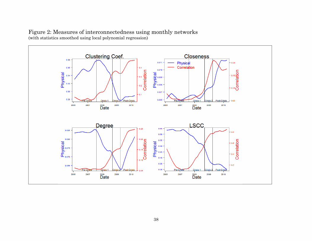
Figure 2 displays the monthly time series of the network measures from the

two types of networks and clearly shows that connectivity increases in the correlation

network at the onset of the first crisis sub-period and keeps rising in the subsequent

sub-periods. Overall, we find that interconnectedness increases after the failure of

Lehman Brothers in the correlation network, but decreases in the physical network.

Lagunoff and Schreft (1998) claim that: “A financial crisis is a breakdown of the

economy’s financial linkages, a collapse of all or part of the financial structure.” (p 2).

The physical network clearly captures this phenomenon.

The two networks also behave differently in other respects. As Figure 3 shows,

correlation networks are sparser than the physical networks in the pre-crisis period,

perhaps expected with only 29 banks in the correlation network. Despite the lower

number of banks, however, the correlation network becomes more interconnected

throughout our sample period. Conversely, the physical network in the post-crisis

period is characterized by a “core” of banks highly interconnected and several banks

which have a low degree of interconnectedness.

To further study the evolution of the two network structures during the crisis,

we identify individual banks that contribute most to market connectivity using the

matrix factorization-based technique developed in Mankad and Michailidis (2013)

and Mankad, Michailidis, and Brunetti (2014).18 Figure 4 displays the importance of

each bank over time and shows that a small subset of banks contributed most to

18 The key idea is to estimate a sequence of low-rank matrix decompositions of the adjacency matrix at each point in time to discover the low-rank latent structure that characterizes the dynamics of the network. We briefly review this technique in the appendix.

20

physical network connectivity during the crisis and beyond. Interestingly, some

banks became more connected in the physical network even while the overall market

became less connected. However, in the correlation network, the onset of the crisis

brought a spike in connectivity among all bank returns. Clearly, physical and

correlation networks have different dynamics.

6. Economic Shocks and Network Connectedness

We explore these differing dynamics further by analyzing how these network

structures reflect economic shocks. Given that markets react to announcements (e.g.

Faust, Rogers, Wang and Wright, (2007)), we aim to compare and contrast how

announcements are reflected in the stock market and interbank market. We are

particularly interested in two types of shocks. The first type refers to European

Central Bank (ECB) announcements and interventions. During our sample period,

the ECB adopted both conventional and unconventional monetary interventions. In

particular, for the ECB interventions19 we distinguish among Long Term Refinancing

Operations (LTRO), Main Refinancing Operations (MRO) and Other Type (OT) of

ECB operations. For the announcements, we follow Rogers, Scotti and Wright (2014)

and consider conventional and unconventional ECB operations.

The second type of shocks we consider refer to more general changes in

macroeconomic conditions. We first capture these shocks using the real activity

indices developed in Scotti (2013): the surprise and uncertainty indices. The surprise

19 These data are available from the ECB website.

21

index summarizes recent economic data surprises and captures optimism/pessimism

about the state of the economy. The uncertainty index measures uncertainty related

to the state of the economy.20 We also consider the evolution of the European stock

market (the Dow-Jones index for Europe) and the London Interbank Offered Rate

(LIBOR).

To fully capture the ECB shocks we use daily data. Hence, for this exercise we

adopt daily networks. Following Kilian and Vega (2011), we estimate the following

models for each sub-period and for each network type:

(12)

(13)

where represents network statistics (closeness, clustering coefficient, degree and

LSCC) on day t, is the economic uncertainty index and the economic surprise

index from Scotti (2013), is the DJ Europe stock index, is the Euro Over

Night Index Average, is a dummy for ECB Long Term Refinancing Operations,

is a dummy for ECB Main Refinancing Operations, is a dummy for Other

Type of ECB operations, and is a dummy variable which captures

both conventional and unconventional ECB intervention announcements.21 , ,

20 The indices, on a given day, are weighted averages of the surprises or squared surprises from a set of macro releases, where the weights depend on the contribution of the associated real activity indicator to a business condition index. 21 The announcements variable is constructed from Rogers, Scotti and Wright (2014) Table 3 data.

22

and are proxies for fundamentals shocks in the economy while ,

, and captures monetary policy shocks.

Figure 5 shows the for each network type, over all dependent variables and

forecasting horizons, k, for equation (12).22 With the exception of the last row (LSCC),

it seems that both networks capture the same information before the crisis. However,

there is a clear pattern showing that the physical network reacts more to ECB

interventions and macro-economic shocks during the crisis and following.

Figure 6 shows the estimated coefficients for the regressions in equation (12).

The correlation network reacts to shocks captured by the which plays an

important role in explaining the structure of the correlation network in all sub-

periods. EONIA and the uncertainty index are the most important factors in the

physical network and seem so dominant that they overshadow the other variable

effects.23 This evidence is consistent with the vast literature showing that uncertainty

has important effects on the real economy.24 Our evidence shows that the network

structures we study react to uncertainty shocks as well.

Indeed, Figure 7 displays the partial from equation (12) related to the

announcements alone (during the pre-crisis period, no announcement were made).

Importantly, early in the crisis the incremental information impounded by the

announcements, conditional on the general impact of macroeconomic factors, is

22 Results for equation (13) are very similar. 23 Similar results are obtained when estimating equation (13). 24 Bloom (2009), e.g., shows that higher uncertainty causes firms to reduce investment and to hire fewer workers. Leduc and Liu (2012) provide evidence that uncertainty in the recent crisis has reduced economic activity and incrementally increased US unemployment by more than one percent.

23

contemporaneously reflected in the correlation network. This conditional impact is

reflected only with a lag in the physical network. However, the magnitude of the

impact in the physical market is often significantly larger for the physical network.

In Figure 8, we distinguish between macroeconomic shocks and monetary

policy shocks (of course the two might be correlated) and formally test whether the

network structure of the correlation and of the physical networks react to these two

types of shocks. Our null hypotheses are that all macro shocks have no effect on the

network structure (i.e. the coefficient of , , and in equations (12)

and (13) are jointly equal to zero), and, similarly, all ECB shocks have no impact on

the network structure (i.e. the coefficients of , and in Equation (12)

are jointly equal to zero in equation (12), and the coefficient for in

equation (13) is equal to zero). A p-value close to zero indicates rejection of the null—

e.g. macro and/or ECB shocks are statistically relevant. In the pre-crisis period,

macroeconomic shocks are important for the correlation network metrics (except in-

degree) at all forecasting horizons, while the physical network reacts to

macroeconomic shocks only at the 3-5 day horizon.

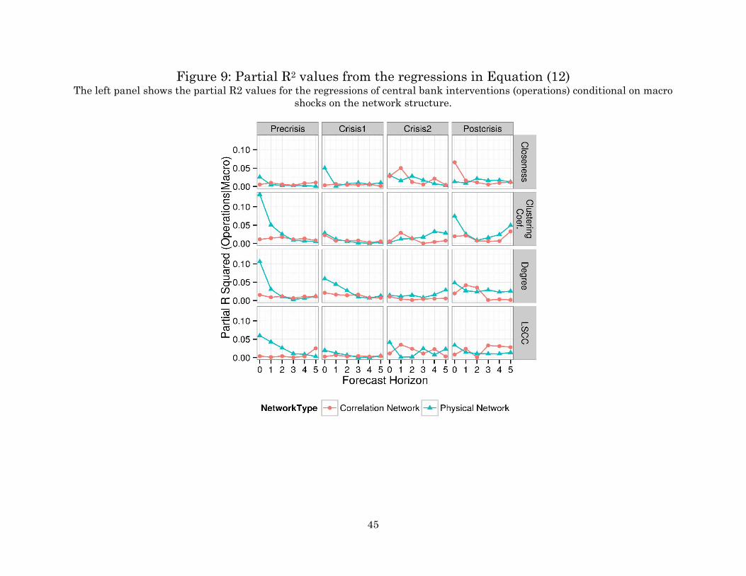
Similarly, Figure 9 documents the partial from equation (12) related to the

operations alone during our sample period. Conditional on the macroeconomic

environment, the physical network generally responds more to central bank

operations. During the pre-crisis period, the incremental explanatory power from

operations in the physical network is greatest contemporaneously, tailing off over

24

subsequent months. During the crisis periods and beyond these effects are

diminished or negligible (depending on the connectedness metric).

In the crisis and post-crisis periods, the physical network is more responsive

to macroeconomic shocks than the correlation network, consistent with Puliga,

Caldarelli, and Battiston (2014) who document that during the crisis increased

correlations in credit default swap premia depend on macroeconomic factors. The F-

tests for the ECB interventions in equation (12) show that these types of shocks are

important to only physical networks. In particular, the physical network reacts to

ECB interventions mainly at short horizons from 0 to 3 days.25

To further isolate the effect of ECB shocks, we also examine the hypotheses

above within a partial regression analysis setting. Specifically, let | : denote the

fitted values resulting from estimating the following regression model

1 2 3 4 1 . (14)

We test the significance of variables in the following regression models

| : 0 5 6 7 (15)

| : 0 5 . (16)

Figure 10 depicts the F-test for the null : 0| , , , 0 for

equation (15). In all sub-periods, the correlation network responds to ECB

interventions only contemporaneously (i.e. k = 0). This is also true for the physical

network. However, interconnectedness in the physical network (measured by the

25 We obtain similar results when analyzing F-tests for the macro and ECB shocks in equation (13) where ECB shocks refer to ECB conventional and unconventional monetary policy announcements.

25

clustering coefficient and degree) reacts to ECB interventions contemporaneously

and across subsequent days in the crisis and post-crisis sub-periods.26

Overall, Figures 5-10 show that the physical and correlation networks respond

differently to shocks and therefore reflect different information sets. To the extent

that correlation networks based on stock prices are more forward looking, we

conjecture that the relatively muted response is related to anticipated macroeconomic

changes. Conversely, since our physical networks respond more strongly to shocks,

we surmise that the physical network more closely reflects connectedness between

and among banks, a connectedness that is more sensitive to economic shocks.

Given that correlation and physical networks capture different phenomena, we

assess whether and how the network topology might help to serve policy makers in

forecasting relevant macroeconomic variables. In this regard, we utilize monthly

networks and consider several of macro variables including

hard information, such as Industrial Production (IP) and Retail Sales (RS);

soft information, such as the Purchasing Manager Index (PMI) —Bańbura and

Rünstler (2011) show that soft information may be important in forecasting);

the spread between the Euro Interbank Offer Rate (EURIBOR) and the

Overnight Indexed Swap (OIS) which is considered to be a measure of health

of the banking system;

26 Similar results are obtained for test-statistic corresponding to the partial regression null hypothesis : 0| , , , 0 in equation (16).

26

the spread between the 10-year Italian, Spanish, Greek and Portuguese

government bond yields and the German government bonds yield, denoted by

ITSP, SPSP, GRSP and PYSP, respectively.27

We estimate the following model from January 2006 until December 2008 (36

months) and then produce one-step-ahead forecasts for the macro-variable from

January 2009 until March 2010.

, , , , , , ,

where , represents the macro-variable described above (we consider one variable

per time) and j denotes the correlation and the physical network, respectively.

Table 4 reports the R2 of the regressions (from January 2006 until December 2008)

and Root Mean Squared Error (RMSE) for the forecasting exercise.

The results show that both the correlation and the physical networks exhibit

statistically similar R2 for the regression of the network variables (Degree, CC,

Closeness and LSCC) on hard information—i.e. Industrial Production (IP), Retail

Sales (RS). This is also the case for the spread between the EURIBOR and the

Overnight Indexed Swap and the Italian spread.

The physical network is able to better explain, in terms of R2, soft information

and the Spanish, Greek and Portuguese spreads. Lastly, the correlation and the

physical networks have similar forecasting performance for industrial production, the

EURIBOR-OIS spread and the Italian spread. However, the physical network is

better suited for forecasting all the other macro variables. For policy makers, the

27 Some of the macro variables are not stationary, in these cases we consider the first difference.

27

interbank market appears to provide valuable information about the future state of

the economy. In this regard, we suggest that monitoring interbank markets would

provide valuable gauge for assessing the state of the bank sector and effectiveness of

interventions.

7. Concluding Remarks

During the recent financial crisis, market dynamics changed dramatically,

with some markets seizing up as market uncertainty and asymmetric information

between banks created unprecedented problems in the world economy. In this paper

we analyze the detailed trading data from the European (e-MID) interbank market

to better understand how interbank trading reflected these economic problems. We

construct and examine physical networks of trade that allow us to examine bank

connectedness over time. Further, we compare and contrast correlation networks

(constructed with Granger-causality between stock returns) with physical networks

(constructed from interbank trades) to better interpret results from each.

We demonstrate that correlation and physical networks reflect important, but

different, economic conditions in the European banking sector. During the crisis,

physical bank networks reveal a breakdown in connectivity in the interbank market.

Interestingly, correlation networks show increased co-movements in market returns

during the crisis that have been interpreted as an increase in connectivity, a

connectivity that we ascribe to a common factor unrelated to interbank trading.

28

Moreover, correlation and physical networks respond differently to monetary

and macroeconomic shocks. Interconnectedness in physical networks adjusts strongly

and quickly to central bank operations and to announcements of new information,

revealing important markers of liquidity at short (daily) horizons. Conversely, while

interconnectedness in correlation networks marks the onset of the crisis, this metric

changes little in response to central announcements and interventions.

Our results demonstrate that correlation networks can identify (and forecast)

periods of impending financial crises. Complementarily, physical interbank trading

networks serve to identify weakening interconnectedness in the interbank system

that may lead to liquidity problems. Moreover, physical networks can identify

systemically important and problem banks on an on-going basis. From a policy

perspective, monitoring both types of networks would be useful.

29

References

Acemoglu, D., O. Asuman and A. Tahbaz-Salehi, 2013. Systemic Risk and Stability in Financial Networks. NBER Working Paper, No. 18727

Acharya, V., L.H. Pedersen, T. Philippon, and M. P. Richardson, 2010. FRB of Cleveland Working

Paper No. 10-02 Acharya V., T. Yorulmazer, 2008. Cash-in-the-Market Pricing and Optimal Resolution of Bank

Failures, Review of Financial Studies 21, 2705-2742. Achlioptas, D., Clauset, A., Kempe, D., & Moore, C. (2009). On the bias of traceroute

sampling: Or, power-law degree distributions in regular graphs. Journal of the ACM 56, 21.

Adrian, T. and H-S. Shin, 2010. Liquidity and Leverage. Journal of Financial

Intermediation 19, 418-437. Allen, F., and A. Babus, 2010. Networks in Finance. In Network-based Strategies and

Competencies, edited by Paul Kleindorfer and Jerry Wind, Wharton School Publishing.

Allen, F. and D. Gale, 2000. Financial Contagion. Journal of Political Economy 108, 1-33. Allen, F., A. Babus and E. Carletti, 2010. Financial Connections and Systemic Risk.

National Bureau of Economic Research, working paper 11177. Bańbura, M., and G. Rünstler, 2011. A look into the factor model black box: publication lags

and the role of hard and soft data in forecasting GDP. International Journal of Forecasting 27, 333-346.

Barigozzi,, M. and C. T. Brownlees, NETS: Network Estimation for Time Series (May 18,

2014). Available at SSRN: http://ssrn.com/abstract=2249909 or http://dx.doi.org/10.2139/ssrn.2249909

Billio, M., M. Getmansky, A. Lo and A. Pelizzon, 2012. Econometric measures of

connectedness and systemic risk in the finance and insurance sectors. Journal of Financial Economics 104, 535-559.

Bloom, N., 2009. The impact of uncertainty shocks. Econometrica 77, 623-685. Braverman, A. and A. Minca, Networks of Common Asset Holdings: Aggregation and

Measures of Vulnerability (January 17, 2014). Available at SSRN: http://ssrn.com/abstract=2379669 or http://dx.doi.org/10.2139/ssrn.2379669

Brunetti, C., M. di Fillippo and J. H. Harris, 2011. Effects of Central Bank Intervention on

the Interbank Market during the Sub-Prime Crisis. Review of Financial Studies 24, 2053-2083.

30

Cabrales, A., P. Gottardi, and F. Vega-Redondo, 2014. Risk-sharing and Contagion in Networks (March 16, 2014). CESifo Working Paper Series No. 4715. Available at SSRN: http://ssrn.com/abstract=2425558.

Caccioli, F., J.D. Farmer, N. Foti and D. Rockmore, 2013. How interbank lending amplifies

overlapping portfolio contagion: A case study of the Austrian banking network. arXiv preprint, arXiv:1306.3704.

Chandrasekaran, V., Parrilo, P. A., & Willsky, A. S. (2012). Latent Variable Graphical

Model Selection via Convex Optimization. Annals of Statistics 40, 1935-1967. Cifuentes, R., C. Ferrucci and H.S. Shin, 2005. Liquidity Risk and Contagion. Journal of

European Economic Association 3, 556-566. Cont, R. and L. Wagalath, Fire Sales Forensics: Measuring Endogenous Risk (May 4, 2012).

Available at SSRN: http://ssrn.com/abstract=2051013 Cont, R. and L. Wagalath, 2013. Running for the Exit: Distressed Selling and Endogenous

Correlations in Financial Markets. Mathematical Finance 23, 718-741. Cont, R., A. Moussa and E. B. Santos, 2013. Network Structure and Systemic Risk in

Banking Systems. Handbook of Systemic Risk. Editor(s): Fouque, Langsam, Cambridge University Press.

De Vries, C., 2005. The Simple Economics of Bank Fragility. Journal of Banking and

Finance 29, 803-825. Delpini, D., S. Battiston, M. Riccaboni, G. Gabbi, F. Pammolli and G. Caldarelli, 2013.

Evolution of Controllability in Interbank Networks. Scientific Report 3, 1626. Diebold, F. X. and K. Yilmaz, 2014. On the network topology of variance decompositions:

Measuring the connectedness of financial firms. Journal of Econometrics 182, 119-134

Elliott, M., B. Golub and M. O. Jackson, 2014. Financial Networks and Contagion.

American Economic Review 104, 3115-53. Elsinger, H., A. Lehar and M. Summer, 2006. Risk Assessment for Banking Systems.

Management Science 52, 1301-1314. Forbes, K.J. and R. Rigobon, 2002. No Contagion, only Interdependence: Measuring Stock

Market Co-movements. Journal of Finance 57, 2223-2261. Faust, J., J. H. Rogers, S.-Y. B. Wang and J. H. Wright, 2007. The high-frequency response

of exchange rates and interest rates to macroeconomic announcements. Journal of Monetary Economics 54, 1051-1068.

Gai, P., A. Haldane and S. Kapadia, 2011. Complexity, Concentration and Contagion.

Journal of Monetary Economics 58, 453-470.

31

Handcock, M. S., & Gile, K. J. (2010). Modeling social networks from sampled data. The Annals of Applied Statistics 4, 5-25. Hatzopoulos, V., G. Iori, R.N. Mantegna, S. Micciche and M. Tumminello, 2014.

Quantifying preferential trading in the e-MID interbank market. Quantitative Finance, ISSN 1469-7688 (In Press).

Iori, G., R.N. Mantegna, L. Marotta, S. Micciche', J. Porter and M. Tumminello, 2014.

Networked relationships in the e-MID Interbank market: A trading model with memory. Journal of Economic Dynamics and Control 50, 98-116.

Jackson, M. 2008. Social and Economic Networks. Princeton University Press, Princeton,

NJ, USA. Kilian, L. and C. Vega, 2011. Do Energy Prices Respond to U.S. Macroeconomic News? A

Test of the Hypothesis of Predetermined Energy Prices, The Review of Economics and Statistics, MIT Press 93, 660-671, May.

Lagunoff, R. and L. Schreft, 2001. A Model of Financial Fragility. Journal of Economic

Theory 99, 220-264. Leduc, S. and Z. Liu, 2012. Uncertainty, unemployment, and inflation. Federal Reserve

Bank of San Francisco Working Paper Series. Mankad, S. and G. Michailidis, 2013. Structural and functional discovery in dynamic

networks with non-negative matrix factorization, Physical Review E 88, 1-14. Mankad, S., G. Michailidis and C. Brunetti, 2014. Visual Analytics for Network-Based

Market Surveillance. DSMM 2014, in conjunction with ACM SIGMOD. Newman, M., Networks: An Introduction, 2010. Oxford University Press

Puliga, M., G. Caldarelli and S. Battiston, 2014. Credit Default Swaps networks and systemic risk. Scientific Reports, 4:6822.

Rogers, J. H., C. Scotti, and J. H. Wright, 2014. Evaluating Asset-Market Effects of

Unconventional Monetary Policy: A Cross-Country Comparison, International Finance Discussion Papers 1101, Board of Governors of the Federal Reserve System (U.S.).

Roukny, R., H. Bersini, H. Pirotte, G. Caldarelli and S. Battiston, 2013. Default Cascades in

Complex Networks: Topology and Systemic Risk. Scientific Reports, 3:2759. Scotti, C., and Board of Governors of the Federal Reserve System (2013). Surprise and

Uncertainty Indexes: Real-Time Aggregation of Real-Activity Macro Surprises, International Finance Discussion Papers 1093. Board of Governors of the Federal Reserve System (U.S.).

32

Shaffer, S., 1994. Pooling Intensify Joint Failure Risk. Research in Financial Services 6,

249-280. Shin, H-S., 2009a. Securitisation and Financial Stability. Economic Journal 119, 309-332. Shin, H-S., 2009b. Financial Intermediation and the Post-Crisis Financial System. BIS

Annual Conference. Upper, C., 2006. Contagion Due to Interbank Credit Exposures: What Do We Know, Why

Do We Know It, and What Should We Know? Working paper, Bank for International Settlements.

33

Table 1 Summary Statistics: Daily Rates of Stock Returns (× 100)

Pre-crisis: 2-Jan-06 - 8-Aug-07

Mean Median St. Dev.

0.4738 0.3160 5.3668 Crisis 1: 9-Aug-07 - 12-Sep-08

-3.8898*** -2.4040 8.4637

Crisis 2: 16-Sep-08 - 1-Apr-09

-9.1711*** -8.5767 22.061

Post-Crisis: 2-Apr-09 - 31-Mar-10

2.4379** 0.1933 12.427

*, ** and *** refer to significance levels of 10%, 5% and 1% for testing the mean difference between each sub-period and the pre-crisis period which we use as benchmark. Standard errors are computed using bootstrapping.

34

Table 2 Summary Statistics: Daily e-MID Financial Variables Pre-crisis: 2-Jan-06 - 8-Aug-07 Mean Median St. Dev. ∆(Price) -0.0232 -0.0150 0.0871 Effective Spread 1.3782 1.3888 0.0988 Volume 22,834 22,337 4,902 Trade Imbalance 0.0049 0.0046 0.0018 Herfindahl Index 0.0159 0.0157 0.0014 Signed Volume -13,154 -12,715 5,631 Crisis 1: 9-Aug-07 - 12-Sep-08

∆(Price) -

0.1236*** -0.0600 0.2224 Effective Spread 1.3685 1.3804 0.1015 Volume 14,512*** 14,132 3,537 Trade Imbalance 0.0067*** 0.0064 0.0024 Herfindahl Index 0.0173** 0.0169 0.0022 Signed Volume -8,777*** -8,591 3,467 Crisis 2: 16-Sep-08 - 1-Apr-09

∆(Price) -

0.2832*** -0.2500 0.2566 Effective Spread 1.3629 1.3754 0.0939 Volume 7,796*** 7,763 2,568 Trade Imbalance 0.0078*** 0.0072 0.0027 Herfindahl Index 0.0202*** 0.0199 0.0026 Signed Volume -4,351*** -4,014 2,180 Post-Crisis: 2-Apr-09 - 31-Mar-10

∆(Price) -

0.1039*** -0.0700 0.1359 Effective Spread 1.3676 1.3772 0.1043 Volume 4,395*** 4,162 1,550 Trade Imbalance 0.0105*** 0.0098 0.0042 Herfindahl Index 0.0240*** 0.0231 0.0040 Signed Volume -2,578*** -2,279 1,464 Trade imbalance is computed as the difference between number of buys and number of sells, normalized by volume. Signed volume is computed as the difference between aggressive buy volume and aggressive sell volume. *, ** and *** refer to significance levels of 10%, 5% and 1% for testing the mean difference between each sub-period and the pre-crisis period which we use as benchmark. Standard errors are computed using bootstrapping.

35

Table 3 Summary Statistics: Monthly Networks Correlation Network Physical Network

Pre-crisis Pre-crisis

2-Jan-06 - 8-Aug-07 2-Jan-06 - 8-Aug-07 Mean Median St. Dev. Mean Median St. Dev. CC 0.0577 0.0492 0.0497 0.3546 0.3524 0.0255 Closeness 0.0571 0.0536 0.0116 0.0064 0.0061 0.0009 Degree 0.0587 0.0582 0.0083 0.0845 0.0843 0.0049 LSCC 0.2201 0.2083 0.1440 0.6318 0.6341 0.0381

Crisis 1 Crisis 1 9-Aug-07 - 12-Sep-08 9-Aug-07 - 12-Sep-08

CC 0.1135*** 0.1026 0.0516 0.3601 0.3651 0.0277 Closeness 0.0564 0.0574 0.0192 0.0063 0.0066 0.0007 Degree 0.0721* 0.0583 0.0365 0.0761*** 0.0774 0.0067 LSCC 0.2279 0.2593 0.1136 0.5632*** 0.5786 0.0525 Crisis 2 Crisis 2 16-Sep-08 - 1-Apr-09 16-Sep-08 - 1-Apr-09 CC 0.3249*** 0.3544 0.3544 0.2930*** 0.2822 0.0351 Closeness 0.1327*** 0.1009 0.1009 0.0071 0.0074 0.0013 Degree 0.1381*** 0.1292 0.1292 0.0663*** 0.0657 0.0064 LSCC 0.6365*** 0.6429 0.6429 0.3800*** 0.0064 0.0624 Post-crisis Post-crisis 2-Apr-09 - 31-Mar-10 2-Apr-09 - 31-Mar-10 CC 0.3074*** 0.3291 0.1369 0.2863*** 0.2818 0.0189 Closeness 0.1360*** 0.1181 0.0725 0.0109*** 0.0110 0.0022 Degree 0.1561*** 0.1700 0.0709 0.0742*** 0.0753 0.0104 LSCC 0.5952*** 0.7143 0.2697 0.3524*** 0.3290 0.0624 CC indicates the clustering coefficient. Closeness measures the average distance, in terms of edges, between banks in the network. Degree refers to the average degree in each network. LSCC refers to the proportion of nodes in the largest strongly connected component. *, ** and *** refer to significance levels of 10%, 5% and 1% for testing the mean difference between each sub-period and the pre-crisis period which we use as benchmark. Standard errors are computed using bootstrapping.

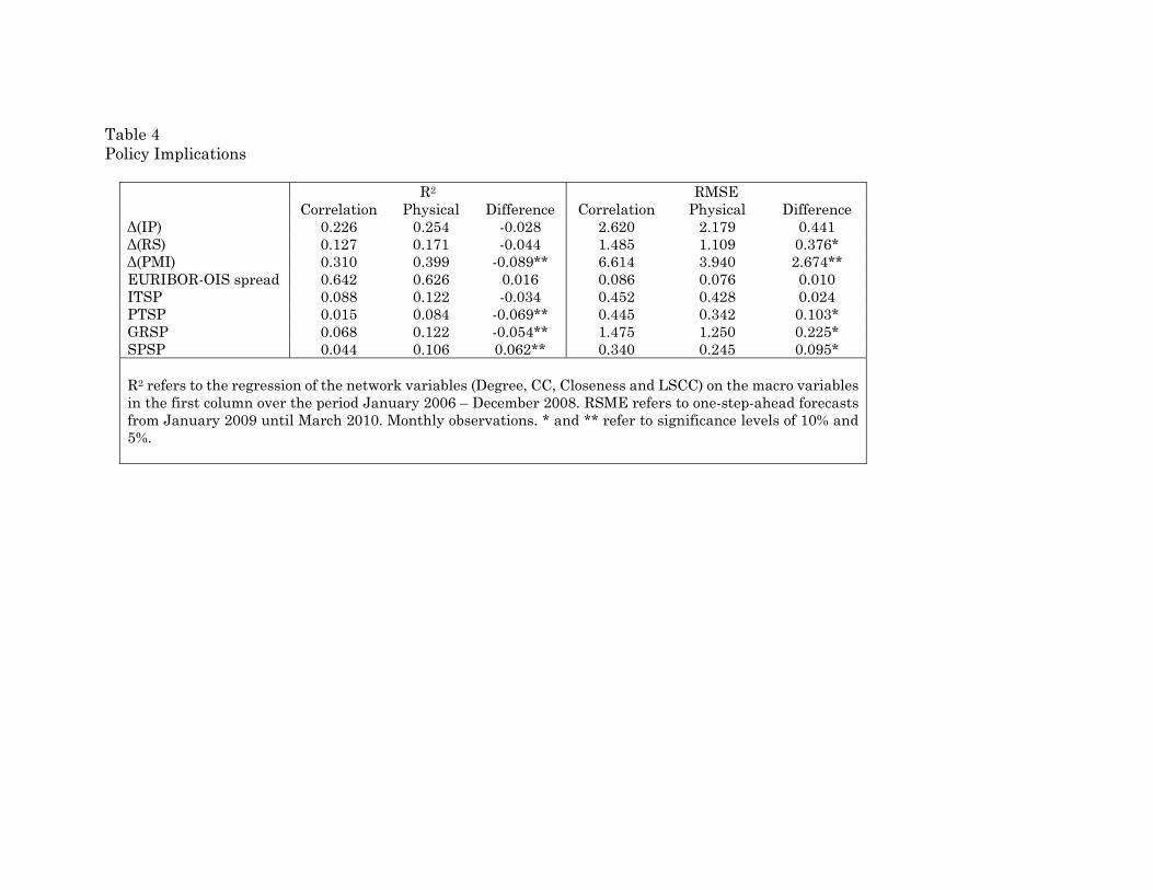
Table 4 Policy Implications

R2 RMSE Correlation Physical Difference Correlation Physical Difference Δ(IP) 0.226 0.254 -0.028 2.620 2.179 0.441 Δ(RS) 0.127 0.171 -0.044 1.485 1.109 0.376* Δ(PMI) 0.310 0.399 -0.089** 6.614 3.940 2.674** EURIBOR-OIS spread 0.642 0.626 0.016 0.086 0.076 0.010 ITSP 0.088 0.122 -0.034 0.452 0.428 0.024 PTSP 0.015 0.084 -0.069** 0.445 0.342 0.103* GRSP 0.068 0.122 -0.054** 1.475 1.250 0.225* SPSP 0.044 0.106 0.062** 0.340 0.245 0.095* R2 refers to the regression of the network variables (Degree, CC, Closeness and LSCC) on the macro variables in the first column over the period January 2006 – December 2008. RSME refers to one-step-ahead forecasts from January 2009 until March 2010. Monthly observations. * and ** refer to significance levels of 10% and 5%.

37

Figure 1: e-MID Daily Financial Variables

38

Figure 2: Measures of interconnectedness using monthly networks (with statistics smoothed using local polynomial regression)

Figure 3: Time-series of network statistics and corresponding graphs

Correlation Network

Physical Network

Figure 4: Directed bank (node) centrality measures, each trajectory corresponds to a different bank. Four different banks with interesting trajectories are colored.

Correlation Network

Physical Network

41

Figure 5: R2 for the regressions in Equation (12)

where represents network statistics (closeness, clustering coefficient, degree and LSCC), is economic uncertainty index, is the economic surprise index (see, Scotti (2013)), is the DJ Europe stock index, is the libor, is a dummy for ECB Long Term Refinancing Operations announcements, is a dummy for ECB Main Refinancing Operations, and is a dummy for Other Type of ECB operations.

Figure 6: Estimated coefficients from the regressions in Equation (12)

The left panel shows estimated coefficients for the correlation network and the right panel shows estimated coefficients for the physical network. All variables have been normalized.

43

Figure 7: Partial R2 values from the regressions in Equation (12) The left panel shows the partial R2 values for the regressions of central banks announcements conditional on macro shocks on

the network structure.

44

Figure 8: P-values from F-Tests for the regressions in Equation (12)

The left panel shows the p-value for the test statistic corresponding to the null hypothesis : 0 – macro shocks do not affect the network structure. The right panel shows the p-value for the test-statistic corresponding to :

0 –ECB interventions do not affect the network structure.

45

Figure 9: Partial R2 values from the regressions in Equation (12) The left panel shows the partial R2 values for the regressions of central bank interventions (operations) conditional on macro

shocks on the network structure.

46

Figure 10: P-values from Conditional Tests for the regressions in Equations (15) The figure shows the p-value for the test statistic corresponding to the partial regression null hypothesis :0| , , , 0 – ECB interventions do not affect the network structure conditional on the macroeconomic variables.

Appendix Let be the network adjacency matrix at time t. Then the given network sequence can be approximated with

, where and are both vectors that are constrained to be non-negative, i.e., each element of and is greater than or equal to zero. Interpretations of and are straight-forward. The j-th element of measures the importance of bank j to average outgoing connectivity at time t. Likewise, the j-th element of measures the importance of bank j to the average incoming connectivity at time t. Together, and are useful for highlighting banks by their importance to interconnectivity. Constraints that force evolving factors and to exhibit temporal smoothness are imposed on the factorizations to enhance their visualization and interpretability. This ensures that bank trajectories are visually smooth when drawn, and as a consequence, time plots of each bank become informative. Thus, centrality measures over time are found by minimizing an objective function that consists of a goodness of fit component and a smoothness penalty

min,∑ || || ∑ || || ∑ || || ,

where the parameters and are set by the user to control the amount of memory or smoothness in the factors over time, and and are both vectors that are constrained to be non-negative. The interpretation is again intuitive. For the physical network, measures importance to selling (outgoing edges) and to buying (incoming edges). For the correlation network, measures importance of banks whose returns are predictive of other bank returns (outgoing edges), and to banks whose stock returns are predicted by other banks’ stock returns (incoming edges). To minimize the objective function and obtain the centrality measures, gradient descent algorithms standard for matrix factorization can be utilized. Extensive discussion, including estimation and other implementation details, can be found in Mankad and Michailidis (2013) and Mankad, Michailidis, and Brunetti (2014).