Embed Size (px)
Citation preview
Interannual variability of the South China Sea
associated with El Nino
Chunzai Wang,1 Weiqiang Wang,2 Dongxiao Wang,2 and Qi Wang3
Received 30 September 2005; revised 23 November 2005; accepted 30 December 2005; published 30 March 2006.
[1] Interannual sea surface temperature (SST) anomalies in the South China Sea (SCS)are largely influenced by El Nino through El Nino–driven atmospheric and oceanicchanges. This paper discovers a new observed feature of the SCS SST anomalies:a double-peak evolution following an El Nino event. The first and second peaks occuraround February and August, respectively, in the subsequent year of the El Nino year(denoted by February [+1] and August [+1]). During and after the mature phase ofEl Nino, a change of atmospheric circulation alters the local SCS near-surface airtemperature, humidity, cloudiness, and monsoon wind. These factors influence surfaceheat fluxes and oceanic flows over the SCS that can either warm or cool the SCSdepending upon stages of SST anomaly evolution. The shortwave radiation and latent heatflux anomalies are major contributions to the first peak of the SCS SST anomalies,although the geostrophic heat advections warm the western boundary region of the SCS.After the first peak of February [+1], both the Ekman and geostrophic heat advections,assisted with a reduction of the net heat flux anomalies, cool the SCS SST anomalies.In August [+1], the mean meridional geostrophic heat advection makes the SCS SSTanomalies peak again. Then, the latent heat flux anomalies (mainly attributed toanomalous air-sea difference in specific humidity) and the mean zonal geostrophic heatadvection take over for the cooling of the SCS after the second peak.
Citation: Wang, C., W. Wang, D. Wang, and Q. Wang (2006), Interannual variability of the South China Sea associated with
El Nino, J. Geophys. Res., 111, C03023, doi:10.1029/2005JC003333.
1. Introduction
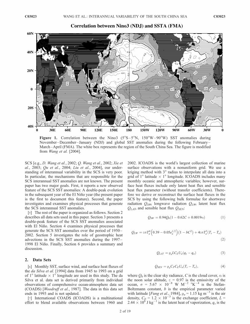
[2] The largest source of Earth’s climate variability in theinstrumental record is El Nino–Southern Oscillation(ENSO). Although ENSO’s maximum sea surface temper-ature (SST) anomalies occur in the equatorial eastern andcentral Pacific, ENSO affects the global ocean. The globalnature of ENSO is shown in Figure 1, which displaysthe correlation between the Nino3 SST anomalies duringNovember–December–January and global SST anomaliesduring the following February–March–April. Theseseasons are chosen because ENSO peaks during the borealwinter while its influence on other ocean basins normallypeaks 1–2 seasons later [e.g., Alexander et al., 2002].Figure 1 shows that outside the tropical Pacific significantENSO-related SST anomalies are found over many places,such as in the tropical North Atlantic, the tropical IndianOcean, the extratropical North and South Pacific, and theSouth China Sea.
[3] The influence of ENSO on other tropical oceans istransmitted through the ‘‘atmospheric bridges’’ of atmo-spheric circulation changes. Using satellite and ship obser-vations and the NCEP-NCAR reanalysis fields, Klein et al.[1999] and Wang [2002, 2005] suggest and show that theWalker and Hadley circulations can serve as an atmosphericbridge. During the warm phase (El Nino) of ENSO, con-vective activity in the equatorial western Pacific shiftseastward. This shift in convection leads to an altered Walkercirculation, with anomalous ascent over the equatorialcentral and eastern Pacific, and anomalous descent overthe equatorial Atlantic and the equatorial Indo-westernPacific region. Thus the Hadley circulation strengthensover the eastern Pacific but weakens over the Atlantic andIndo-western Pacific sectors. These anomalous Walker andHadley circulations result in variations in surface wind, airtemperature, humidity, and cloud cover that in turn influ-ence surface heat fluxes and ocean circulations over otherocean basins and then change SST.[4] The correlation map of Figure 1 shows that the South
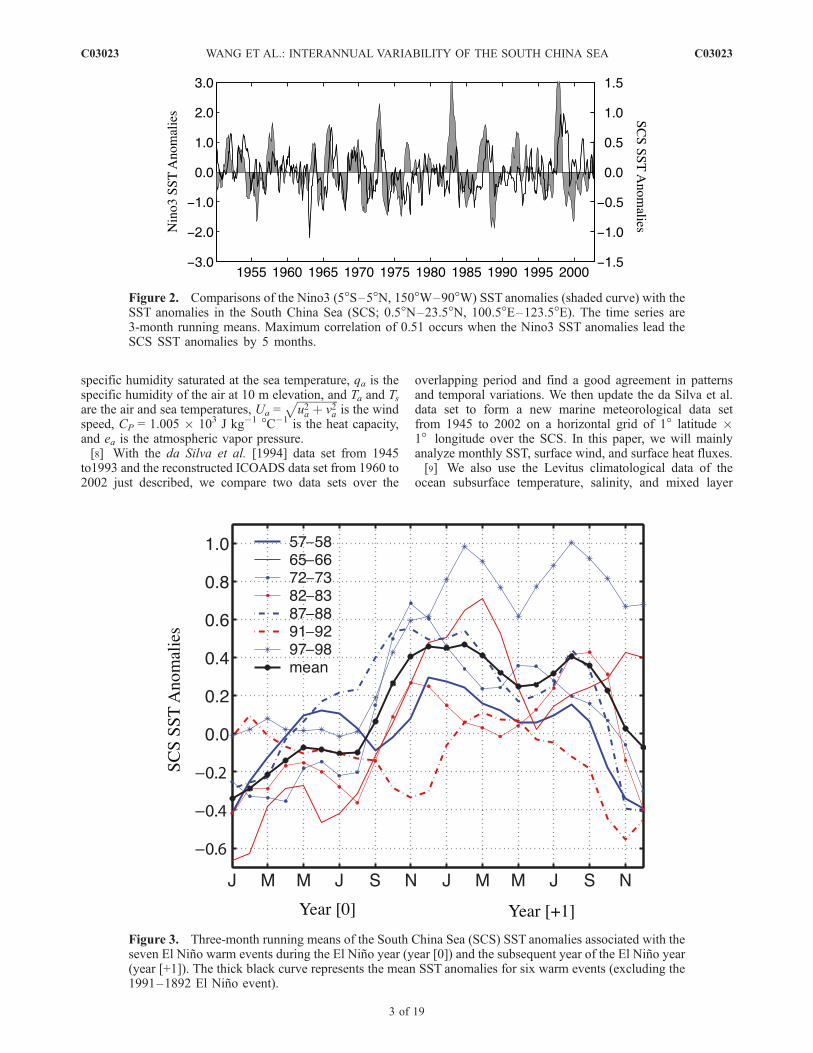
China Sea (SCS) is largely influenced by ENSO. The timeseries of the SCS and Nino3 SST anomalies in all calendarmonths from 1950 to 2002 are compared in Figure 2. EveryENSO event is associated with a change in the SCS SSTanomalies. The calculation shows that maximum correlationof 0.51 occurs when the Nino3 SST anomalies lead the SCSSST anomalies by 5 months [also see Klein et al., 1999;Wang et al., 2000]. In spite of a strong ENSO impact on the
JOURNAL OF GEOPHYSICAL RESEARCH, VOL. 111, C03023, doi:10.1029/2005JC003333, 2006
1Atlantic Oceanographic and Meteorological Laboratory, PhysicalOceanography Division, NOAA, Miami, Florida, USA.
2Key Laboratory of Tropical Marine Environmental Dynamics, SouthChina Sea Institute of Oceanology, Chinese Academy of Sciences,Guangzhou, China.
3Department of Meteorology, Physical Oceanography Laboratory,Ocean University of China, Qingdao, China.
Copyright 2006 by the American Geophysical Union.0148-0227/06/2005JC003333$09.00
C03023 1 of 19
SCS [e.g., D. Wang et al., 2002; Q. Wang et al., 2002; Xie etal., 2003; Qu et al., 2004; Liu et al., 2004], our under-standing of interannual variability in the SCS is very poor.In particular, the mechanisms that are responsible for theSCS interannual SST anomalies are not known. The presentpaper has two major goals. First, it reports a new observedfeature of the SCS SST anomalies: A double-peak evolutionin the subsequent year of the El Nino year (the present paperis the first to document this feature). Second, the paperinvestigates and examines physical processes that generatethe SCS interannual SST anomalies.[5] The rest of the paper is organized as follows. Section 2
describes all data sets used in this paper. Section 3 presents adouble-peak feature of the SCS SST anomalies associatedwith El Nino. Section 4 examines physical processes thatgenerate the SCS SST anomalies over the period of 1950–2002. Section 5 investigates the role of geostrophic heatadvections in the SCS SST anomalies during the 1997–1998 El Nino. Finally, Section 6 provides a summary anddiscussion.
2. Data Sets
[6] Monthly SST, surface wind, and surface heat fluxes ofthe da Silva et al. [1994] data from 1945 to 1993 on a gridof 1� latitude � 1� longitude are used in this study. The daSilva et al. data set is derived primarily from individualobservations of comprehensive ocean-atmosphere data set(COADS) [Woodruff et al., 1987]. The data in this data setends in 1993 and is not updated.[7] International COADS (ICOADS) is a multinational
effort to blend available observations between 1960 and
2002. ICOADS is the world’s largest collection of marinesurface observations with a nonuniform grid. We use akriging method with 3� radius to interpolate all data into agrid of 1� latitude � 1� longitude. ICOADS includes manymonthly oceanic and atmospheric variables; however, sur-face heat fluxes include only latent heat flux and sensibleheat flux parameter (without transfer coefficients). There-fore we derive or reconstruct the surface heat fluxes in theSCS by using the following bulk formulae for shortwaveradiation QSW, longwave radiation QLW, latent heat fluxQLAT, and sensible heat flux QSEN:
QSW ¼ 0:94Q0 1� 0:62C þ 0:0019að Þ ð1Þ
QLW ¼ esT4a 0:39� 0:05e1=2a
� �1� bC2� �
þ 4esT3a Ts � Tað Þ
ð2Þ
QLAT ¼ raLCEUa qs � qað Þ ð3Þ
QSEN ¼ raCPCEUa Ts � Tað Þ; ð4Þ
where Q0 is the clear sky radiance, C is the cloud cover, a isthe noon solar altitude, e = 0.97 is the emissivity of theocean, s = 5.67 � 10�8 W M�2 �K�4 is the Stefan-Boltzmann constant, b is the empirical parameter variedwith latitude [Fung et al., 1984], ra = 1.15 kg m�3 is the airdensity, CE = 1.2 � 10�3 is the exchange coefficient, L =2.44 � 106 J kg�1 is the latent heat of vaporization, qs is the
Figure 1. Correlation between the Nino3 (5�S–5�N, 150�W–90�W) SST anomalies duringNovember–December–January (NDJ) and global SST anomalies during the following February–March–April (FMA). The white box represents the region of the South China Sea. The figure is modifiedfrom Wang et al. [2004].
C03023 WANG ET AL.: INTERANNUAL VARIABILITY OF THE SOUTH CHINA SEA
2 of 19
C03023
specific humidity saturated at the sea temperature, qa is thespecific humidity of the air at 10 m elevation, and Ta and Tsare the air and sea temperatures, Ua =
ffiffiffiffiffiffiffiffiffiffiffiffiffiffiffiu2a þ v2a
pis the wind
speed, CP = 1.005 � 103 J kg�1 �C�1 is the heat capacity,and ea is the atmospheric vapor pressure.[8] With the da Silva et al. [1994] data set from 1945
to1993 and the reconstructed ICOADS data set from 1960 to2002 just described, we compare two data sets over the
overlapping period and find a good agreement in patternsand temporal variations. We then update the da Silva et al.data set to form a new marine meteorological data setfrom 1945 to 2002 on a horizontal grid of 1� latitude �1� longitude over the SCS. In this paper, we will mainlyanalyze monthly SST, surface wind, and surface heat fluxes.[9] We also use the Levitus climatological data of the
ocean subsurface temperature, salinity, and mixed layer
Figure 2. Comparisons of the Nino3 (5�S–5�N, 150�W–90�W) SST anomalies (shaded curve) with theSST anomalies in the South China Sea (SCS; 0.5�N–23.5�N, 100.5�E–123.5�E). The time series are3-month running means. Maximum correlation of 0.51 occurs when the Nino3 SST anomalies lead theSCS SST anomalies by 5 months.
Figure 3. Three-month running means of the South China Sea (SCS) SST anomalies associated with theseven El Nino warm events during the El Nino year (year [0]) and the subsequent year of the El Nino year(year [+1]). The thick black curve represents the mean SST anomalies for six warm events (excluding the1991–1892 El Nino event).
C03023 WANG ET AL.: INTERANNUAL VARIABILITY OF THE SOUTH CHINA SEA
3 of 19
C03023
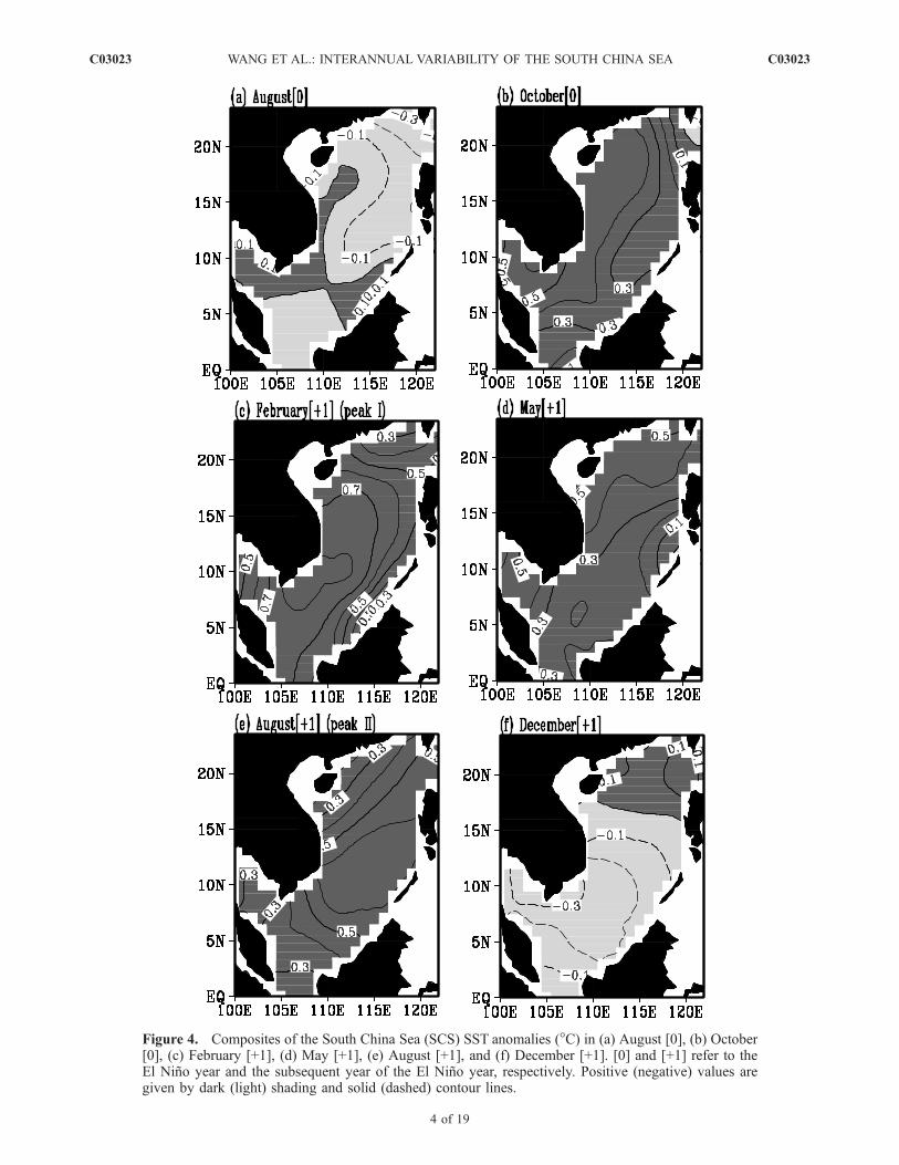
Figure 4. Composites of the South China Sea (SCS) SST anomalies (�C) in (a) August [0], (b) October[0], (c) February [+1], (d) May [+1], (e) August [+1], and (f) December [+1]. [0] and [+1] refer to theEl Nino year and the subsequent year of the El Nino year, respectively. Positive (negative) values aregiven by dark (light) shading and solid (dashed) contour lines.
C03023 WANG ET AL.: INTERANNUAL VARIABILITY OF THE SOUTH CHINA SEA
4 of 19
C03023
depth [Levitus and Boyer, 1994]. The Levitus climatologycomprises quality controlled ocean profile data averagedonto a global 1� latitude � 1� longitude grid at fixedstandard depths.[10] Finally, the sea surface height (SSH) data set that
merges European Remote Sensing (ERS) and TOPEX/Poseidon (T/P) altimetry observations [Ducet et al., 2000]is also utilized. This SSH product is monthly with a grid of0.25� latitude � 0.25� longitude from 1992 to 2001. TheSSH data, assisted with the Levitus climatological data, isused to calculate the geostrophic current in the SCS.[11] With all of these data sets, we first calculate monthly
climatologies on the basis of the full data record period andthen anomalies are obtained by subtracting the monthlyclimatologies from the data. A linear trend removal is
applied to the anomaly data at all grid points before ouranalyses.
3. Double Peak of the SCS SST Anomalies
[12] As stated in the introduction, interannual variabilityof the SCS is largely influenced by El Nino event. From1950 to 2002, there are seven significant El Nino warmevents: 1957–1958, 1965–1966, 1972–1973, 1982–1983,1986–1987, 1991–1992, and 1997–1998. Note that we donot consider the two recent and weak El Ninos of 2002–2003 and 2004–2005 since our data set records do notcover these two events. The maximum Nino3 SST anoma-lies for each warm event occur during the calendar monthsfrom November to January, except for the 1986–1987 El
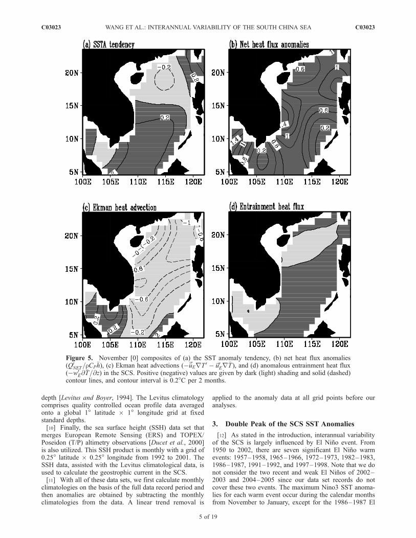
Figure 5. November [0] composites of (a) the SST anomaly tendency, (b) net heat flux anomalies(Q0
NET=rCP�h), (c) Ekman heat advections (�~�uErT 0 �~u0Er�T ), and (d) anomalous entrainment heat flux
(�w0E@�T=@z) in the SCS. Positive (negative) values are given by dark (light) shading and solid (dashed)
contour lines, and contour interval is 0.2�C per 2 months.
C03023 WANG ET AL.: INTERANNUAL VARIABILITY OF THE SOUTH CHINA SEA
5 of 19
C03023
Nino event which has the largest peak in the followingboreal summer (a weak peak in the winter of the El Ninoyear). Corresponding to these El Nino warm events in thePacific, the SCS also shows a warm state. Figure 3 displaysthe SCS SST anomalies associated with the seven El Ninowarm events during the El Nino year and the subsequentyear of the El Nino year. For the 1986–1987 El Nino, theSCS is warm in the winter of 1987 and the summer of1988. Therefore we plot the SCS SST anomalies from 1987to 1988 in Figure 3 for the case of the 1986–1987 El Nino.The SCS SST anomalies begin to warm up in the borealfall of the El Nino year and the warm state lasts for morethan one year. A prominent feature of the SCS SSTanomalies is a double peak following El Nino. For allEl Nino events except the weak 1991–1992 event, the SCSSST anomalies peak two times during the subsequent yearof the El Nino year. In all of the following compositecalculations, we will exclude the weak 1991–1992 event.
The mean SCS SST anomalies for six warm events(excluding the 1991–1992 event; thick black curve inFigure 3) show that the double peak of the SCS SSTanomalies occurs in February [+1] and August [+1], withthe average SST anomalies of 0.47�C and 0.41�C, respec-tively. Note that in this paper, [0] and [+1] refer to the ElNino year and the subsequent year of the El Nino year,respectively.[13] How the horizontal structure of the SCS SST
anomalies evolves can be examined by compositing theSCS SST anomalies during different stages of El Nino, asshown in Figure 4. The SCS is cold in and before August [0](Figure 4a), and the entire SCS becomes warm in October[0] with maximum positive SST anomalies located in thewest half of the basin (Figure 4b). After the basin-scalewarming of October [0], the entire SCS remains warmtoward the next year of November [+1]. The double peakof the SCS SST anomalies is also evidenced in Figure 4 by
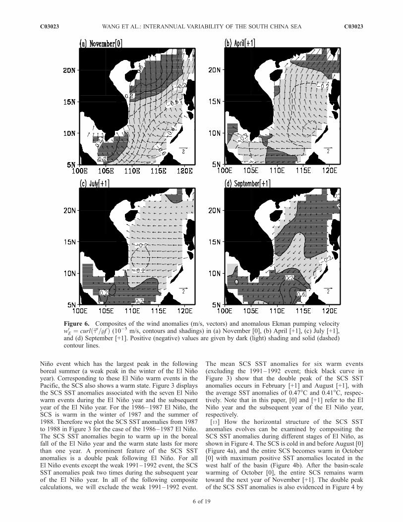
Figure 6. Composites of the wind anomalies (m/s, vectors) and anomalous Ekman pumping velocityw0E ¼ curl ~t0=rfð Þ (10�5 m/s, contours and shadings) in (a) November [0], (b) April [+1], (c) July [+1],
and (d) September [+1]. Positive (negative) values are given by dark (light) shading and solid (dashed)contour lines.
C03023 WANG ET AL.: INTERANNUAL VARIABILITY OF THE SOUTH CHINA SEA
6 of 19
C03023
showing that the SCS SST anomalies reach their maximumin February [+1] (Figure 4c), decay toward May [+1](Figure 4d), and then increase again and peak in August[+1] (Figure 4e). The center of maximum SST anomalies islocated in the southern SCS for the first peak (Figure 4c),whereas it is in the central SCS for the second peak(Figure 4e). After the more than one year warming (the entireSCS is still warm in October [+1]), the SCS returns to a coldstate in December [+1] (Figure 4f).
4. Processes Generating the SCS SST Anomalies
[14] The focus of this paper is on interannual variabilityof SST anomalies over the SCS. After linearizing the SSTequation, we obtain that
@T 0
@t¼ Q0
NET
rCP�h�~�uE rT 0 �~u0E r�T �~�uG rT 0 �~u0G r�T
� w0E
@�T
@z� �wE
@T 0
@z; ð5Þ
where the overbar denotes the climatological mean and theprime denotes anomaly. T is the SST, QNET is the net surface
heat flux, h is the mixed layer depth,~uE ¼ ~t�~k� �
= rf �h� �
is the Ekman velocity vector,~uG is the geostrophic velocityvector, and wE = curl(~t/rf) is the Ekman pumping(entrainment) velocity. The term in the left hand side ofequation (5) is the SST anomaly tendency. The terms in theright hand side of equation (5) are the net heat fluxanomalies, mean Ekman heat advection, anomalous Ekmanheat advection, mean geostrophic heat advection, anom-alous geostrophic advection, anomalous entrainment heatflux, and mean entrainment heat flux, respectively. Non-linear heat advection terms, which are usually small in theSCS, are not considered in this paper.[15] The Levitus climatological ocean temperature data is
used to calculate the mean vertical temperature gradient
@�T=@z. However, we cannot calculate the anomalous ver-tical temperature gradient @T0/@z since it requires long-termocean subsurface temperature data which is not available.Thus we cannot estimate the last term of equation (5). Inthis section, we will focus on the net heat flux anomalies,the Ekman heat advection terms, and the anomalous en-trainment heat flux term, all of which can be estimated fromthe long-record data of 1945–2002. The geostrophic cur-rent, calculated from satellite measurements and the Levitusclimatological data, is available only after 1992. Thus itsadvective role on the SCS SST anomalies during the 1997–1998 El Nino will be considered as a special case study inSection 5.
4.1. First Peak of SST Anomalies
[16] Section 3 shows that the SCS interannual SSTanomalies reach the first peak around February [+1]immediately following the mature phase of El Nino. Sucha warming connection between the SCS and equatorialeastern Pacific is believed to be through El Nino–drivenatmospheric teleconnections that alter the surface heat fluxand winds that in turn change the SST in the SCS. Sincewe are interested in what causes the SCS SST anomaliesto peak, we choose the month of November [0]—prior tothe first peak as a study month. Figure 5 shows theNovember [0] composites of the SST anomaly tendency,net heat flux anomalies, Ekman heat advection terms, andanomalous entrainment heat flux over the SCS. In thispaper, an SST anomaly tendency in a given month iscalculated by the difference between the SST anomaly inthe subsequent month and that in the previous one. Duringthe boreal winter, the local atmospheric condition over theSCS is the northeast monsoon wind. When an El Ninooccurs in the Pacific, the winter northeast monsoon windover the SCS is weakened, resulting in southerly windanomalies, as shown for the case of November [0] inFigure 6a. Thus the mean and anomalous Ekman flows in
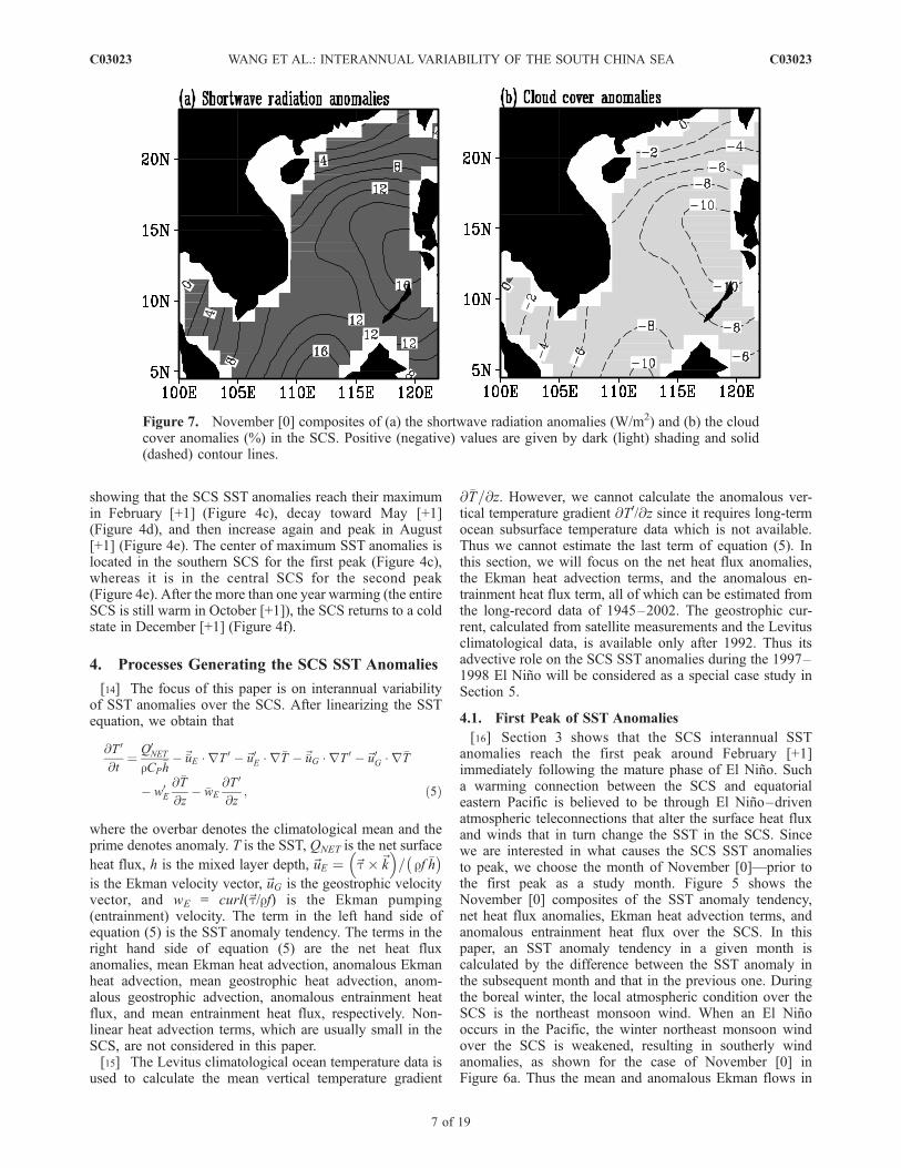
Figure 7. November [0] composites of (a) the shortwave radiation anomalies (W/m2) and (b) the cloudcover anomalies (%) in the SCS. Positive (negative) values are given by dark (light) shading and solid(dashed) contour lines.
C03023 WANG ET AL.: INTERANNUAL VARIABILITY OF THE SOUTH CHINA SEA
7 of 19
C03023

November [0] over the SCS are northwestward andeastward, respectively. These Ekman flows, associatedwith the westward anomalous and southeastward meanSST gradients, induce negative value of the Ekman heat
advections (�~�uErT 0 �~u0Er�T < 0) in Figure 5c. Thisindicates that the Ekman heat advections cool the SCSand cannot account for the warming tendency as shown inFigure 5a. On the other hand, the weakening of thenortheast monsoon wind during the winter of the El Ninoyear corresponds to anomalous downward Ekman pump-ing velocity (Figure 6a) which results in the positiveentrainment heat flux anomalies in the central and south-ern SCS as shown in Figure 5d. However, the amplitudeof the entrainment heat flux anomalies is too small toaccount for the SST warming.[17] The large positive value of the net heat flux anoma-
lies in November [0] suggests that surface heat flux isresponsible for generating the first peak of the SCS SSTanomalies (Figure 5b). The net surface heat flux anomaliesinclude the components of shortwave radiation anomalies,latent heat flux anomalies, sensible heat flux anomalies, andlongwave radiation anomalies. Since the amplitude of thesensible heat flux and longwave radiation anomalies in theSCS is smaller than that of the shortwave radiation andlatent heat flux anomalies (not shown), we only examine theshortwave radiation and latent heat flux anomalies. We firstconsider the distribution of the shortwave radiation anoma-lies. If we linearize equation (1) of the shortwave radiation,we can get that
Q0SW ¼ 0:94Q0 �0:62C0ð Þ: ð6Þ
The shortwave radiation anomaly (QSW0 ) is linearly
determined by the cloud cover anomaly (C0). Figure 7shows the November [0] composites of the shortwaveradiation anomalies and the cloud cover anomalies in theSCS. As expected, the pattern of the shortwave radiationanomalies is the same as that of the cloud cover anomalies,except with an opposite sign. A decrease in the cloudinessover the SCS induces an increase in the shortwave radiation.[18] Latent heat flux is determined by wind speed and air-
sea difference in specific humidity. Linearizing equation (3)results in
Q0LAT ¼ raLCE U 0
aD�qþ �UaDq0� �: ð7Þ
The latent heat flux anomalies are attributed to variations ofthe wind speed anomaly (Ua
0 ) and anomalous air-seadifference in specific humidity (Dq0). Again, equation (7)neglects the nonlinear term of Ua
0Dq0 that is smaller.Figure 8 shows the November [0] composites of the latentheat flux anomalies and the contributions of the wind speedanomaly and of anomalous air-sea difference in specifichumidity to the latent heat flux anomalies. During thewinter of the El Nino year, the northeast monsoon wind
Figure 8. November [0] composites of (a) the latent heatflux anomalies, (b) the contribution of the wind speedanomaly to the latent heat flux anomalies, and (c) thecontribution of anomalous air-sea difference in specifichumidity to the latent heat flux anomalies. Positive latentheat flux indicates that the ocean gives heat to theatmosphere. Units are W/m2. Positive (negative) values aregiven by dark (light) shading and solid (dashed) contourlines.
C03023 WANG ET AL.: INTERANNUAL VARIABILITY OF THE SOUTH CHINA SEA
8 of 19
C03023
over the SCS is weakened, with maximum weakeningoccurring in the northern SCS (Figure 6a). The weakeningof the northeast monsoon decreases the wind speed thatresults in negative heat flux anomalies centered in thenorthern SCS (Figure 8b). On the other hand, thecontribution of anomalous air-sea difference in specifichumidity to the latent heat flux anomalies is positive overthe southern and central SCS (Figure 8c). The combinedeffect is negative (positive) latent heat flux anomalies in thenorthern (southern) SCS (Figure 8a). Note that positivelatent heat flux is defined as heat loss from the ocean. Insummary, the positive net heat flux anomalies in November[0], which are responsible for the SCS warming, mainlyresult from increase in the shortwave radiation anomalies(attributed to cloudiness anomalies) and decrease in thelatent heat flux anomalies (attributed to both the wind speed
anomalies and anomalous air-sea difference in specifichumidity).
4.2. Decay of SST Anomalies Following the First Peak
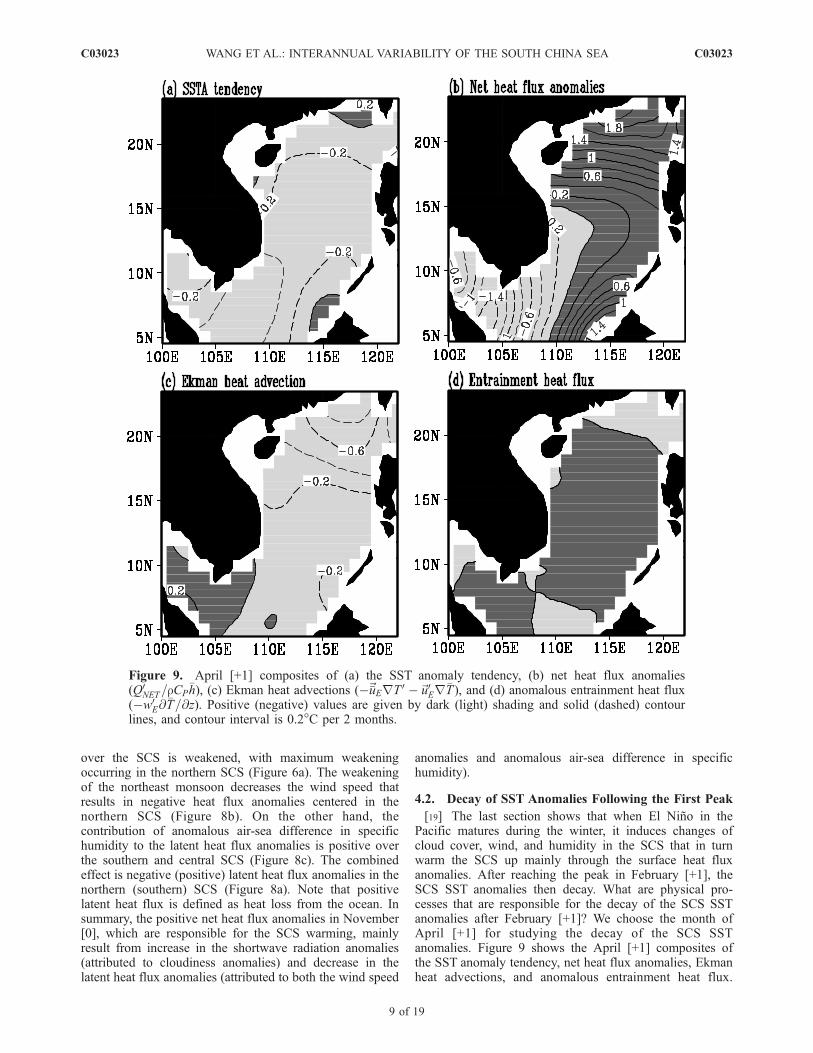
[19] The last section shows that when El Nino in thePacific matures during the winter, it induces changes ofcloud cover, wind, and humidity in the SCS that in turnwarm the SCS up mainly through the surface heat fluxanomalies. After reaching the peak in February [+1], theSCS SST anomalies then decay. What are physical pro-cesses that are responsible for the decay of the SCS SSTanomalies after February [+1]? We choose the month ofApril [+1] for studying the decay of the SCS SSTanomalies. Figure 9 shows the April [+1] composites ofthe SST anomaly tendency, net heat flux anomalies, Ekmanheat advections, and anomalous entrainment heat flux.
Figure 9. April [+1] composites of (a) the SST anomaly tendency, (b) net heat flux anomalies(Q0
NET=rCP�h), (c) Ekman heat advections (�~�uErT 0 �~u0Er�T ), and (d) anomalous entrainment heat flux
(�w0E@
�T=@z). Positive (negative) values are given by dark (light) shading and solid (dashed) contourlines, and contour interval is 0.2�C per 2 months.
C03023 WANG ET AL.: INTERANNUAL VARIABILITY OF THE SOUTH CHINA SEA
9 of 19
C03023
Over most regions of the SCS the net heat flux anomaliesare positive, except for the region of the Sunda shelf andthe South Vietnam coast (Figure 9b). Comparison ofFigure 5b and Figure 9b shows that the net heat fluxanomalies in the central and southwestern SCS are reduced,favoring the decay of SST anomalies. In April [+1], the SCSis still associated with a weakening of the northeast mon-soon with strong southerly wind anomalies in the centraland northern SCS (Figure 6b). Correspondingly, the windpattern produces an anomalous downward Ekman pumpingvelocity (Figure 6b) that results in positive anomalousentrainment heat flux (Figure 9d). Thus the anomalousentrainment heat flux during that time tends to warm theSCS (in spite of a small amplitude).[20] However, the mean and anomalous Ekman heat
advections tend to cool the SCS (Figure 9c). The wind
patterns over the SCS in the subsequent spring of theEl Nino year are similar to those in the winter of theEl Nino year. Similar to the case of November [0], boththe mean northwestward and anomalous eastward Ekmanflows (associated with the mean northeast monsoon andanomalous southerly winds, respectively) in April [+1]contribute to the negative value of the Ekman heat advec-tions shown in Figure 9c. The negative Ekman heat advec-tions, assisted with the reduction of the surface heat fluxanomalies, cool the SCS in April [+1].
4.3. Second Peak of SST Anomalies
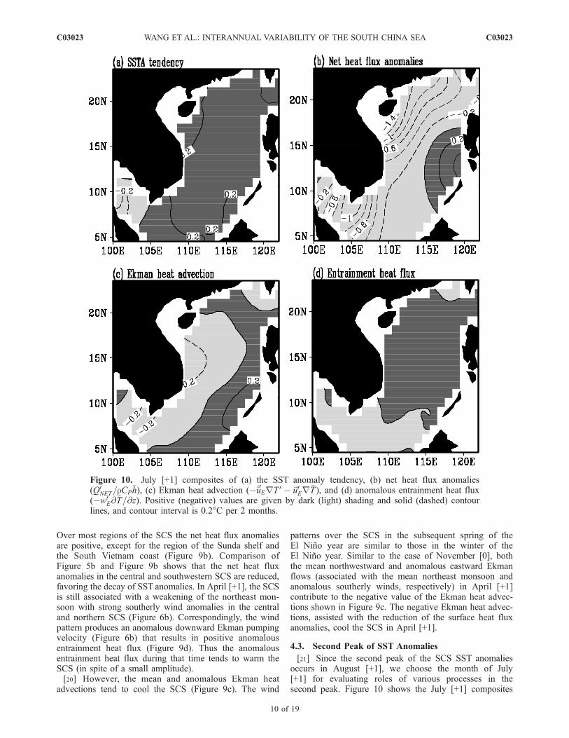
[21] Since the second peak of the SCS SST anomaliesoccurs in August [+1], we choose the month of July[+1] for evaluating roles of various processes in thesecond peak. Figure 10 shows the July [+1] composites
Figure 10. July [+1] composites of (a) the SST anomaly tendency, (b) net heat flux anomalies(Q0
NET=rCP�h), (c) Ekman heat advection (�~�uErT 0 �~u0Er�T ), and (d) anomalous entrainment heat flux
(�w0E@
�T=@z). Positive (negative) values are given by dark (light) shading and solid (dashed) contourlines, and contour interval is 0.2�C per 2 months.
C03023 WANG ET AL.: INTERANNUAL VARIABILITY OF THE SOUTH CHINA SEA
10 of 19
C03023
of the SST anomaly tendency, net heat flux anomalies,Ekman heat advection terms, and anomalous entrainmentheat flux. The net heat flux anomalies are negativealmost everywhere in the SCS (Figure 10b). The Ekmanheat advections are also negative over the western andcentral SCS (Figure 10c). The only process in Figure 10that can warm the SCS is the positive anomalousentrainment heat flux (Figure 10d) that results from adownward anomalous Ekman pumping velocity in July[+1] (Figure 6c). However, the amplitude of the positiveanomalous entrainment heat flux is too small to accountfor the warming of the second peak. This means thatother processes must be responsible for the warming ofthe second peak. Section 5 will show that during the1997–1998 El Nino the geostrophic heat advection is
important for the second SST anomaly peak occurring inAugust of 1998.
4.4. Decay of SST Anomalies Following theSecond Peak
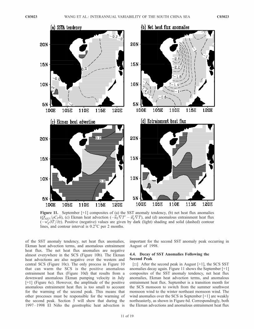
[22] After the second peak in August [+1], the SCS SSTanomalies decay again. Figure 11 shows the September [+1]composites of the SST anomaly tendency, net heat fluxanomalies, Ekman heat advection terms, and anomalousentrainment heat flux. September is a transition month forthe SCS monsoon to switch from the summer southwestmonsoon wind to the winter northeast monsoon wind. Thewind anomalies over the SCS in September [+1] are weaklynortheasterly, as shown in Figure 6d. Correspondingly, boththe Ekman advections and anomalous entrainment heat flux
Figure 11. September [+1] composites of (a) the SST anomaly tendency, (b) net heat flux anomalies(Q0
NET=rCP�h), (c) Ekman heat advection (�~�uErT 0 �~u0Er�T ), and (d) anomalous entrainment heat flux
(�w0E@
�T=@z). Positive (negative) values are given by dark (light) shading and solid (dashed) contourlines, and contour interval is 0.2�C per 2 months.
C03023 WANG ET AL.: INTERANNUAL VARIABILITY OF THE SOUTH CHINA SEA
11 of 19
C03023
are small (Figures 11c and 11d), suggesting that they cannotcool the SCS. The large negative value of the net heat fluxanomalies (Figure 11b) indicates that the surface heat fluxanomalies are responsible for the negative SST anomalytendency in September [+1].[23] Again, we only examine the shortwave radiation and
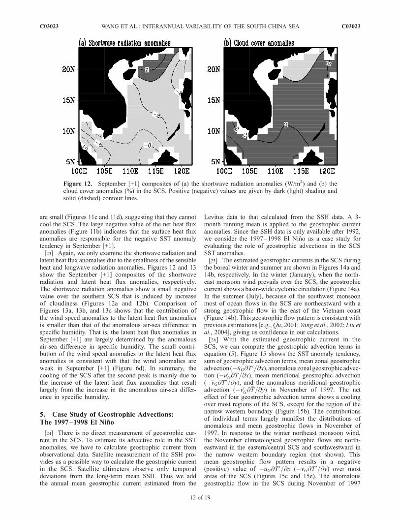
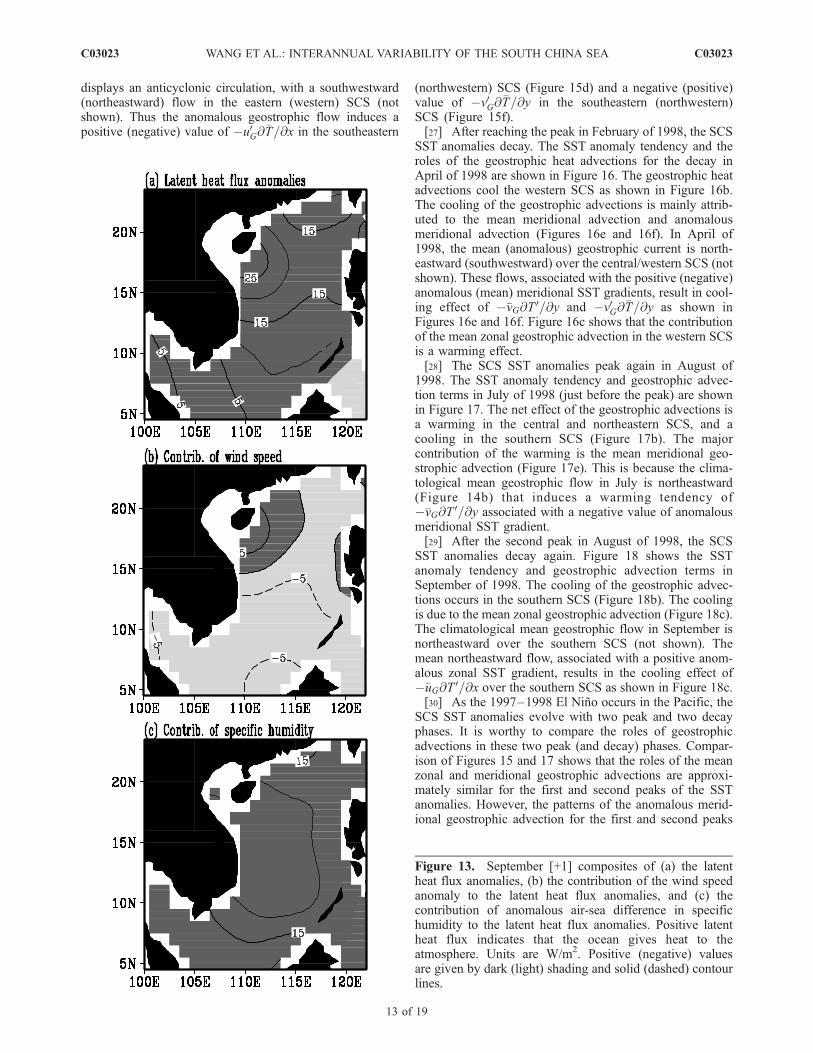
latent heat flux anomalies due to the smallness of the sensibleheat and longwave radiation anomalies. Figures 12 and 13show the September [+1] composites of the shortwaveradiation and latent heat flux anomalies, respectively.The shortwave radiation anomalies show a small negativevalue over the southern SCS that is induced by increaseof cloudiness (Figures 12a and 12b). Comparison ofFigures 13a, 13b, and 13c shows that the contribution ofthe wind speed anomalies to the latent heat flux anomaliesis smaller than that of the anomalous air-sea difference inspecific humidity. That is, the latent heat flux anomalies inSeptember [+1] are largely determined by the anomalousair-sea difference in specific humidity. The small contri-bution of the wind speed anomalies to the latent heat fluxanomalies is consistent with that the wind anomalies areweak in September [+1] (Figure 6d). In summary, thecooling of the SCS after the second peak is mainly due tothe increase of the latent heat flux anomalies that resultlargely from the increase in the anomalous air-sea differ-ence in specific humidity.
5. Case Study of Geostrophic Advections:The 1997–1998 El Nino
[24] There is no direct measurement of geostrophic cur-rent in the SCS. To estimate its advective role in the SSTanomalies, we have to calculate geostrophic current fromobservational data. Satellite measurement of the SSH pro-vides us a possible way to calculate the geostrophic currentin the SCS. Satellite altimeters observe only temporaldeviations from the long-term mean SSH. Thus we addthe annual mean geostrophic current estimated from the
Levitus data to that calculated from the SSH data. A 3-month running mean is applied to the geostrophic currentanomalies. Since the SSH data is only available after 1992,we consider the 1997–1998 El Nino as a case study forevaluating the role of geostrophic advections in the SCSSST anomalies.[25] The estimated geostrophic currents in the SCS during
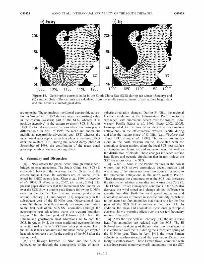
the boreal winter and summer are shown in Figures 14a and14b, respectively. In the winter (January), when the north-east monsoon wind prevails over the SCS, the geostrophiccurrent shows a basin-wide cyclonic circulation (Figure 14a).In the summer (July), because of the southwest monsoonmost of ocean flows in the SCS are northeastward with astrong geostrophic flow in the east of the Vietnam coast(Figure 14b). This geostrophic flow pattern is consistent withprevious estimations [e.g.,Qu, 2001; Yang et al., 2002; Liu etal., 2004], giving us confidence in our calculations.[26] With the estimated geostrophic current in the
SCS, we can compute the geostrophic advection terms inequation (5). Figure 15 shows the SST anomaly tendency,sum of geostrophic advection terms, mean zonal geostrophicadvection (��uG@T
0=@x), anomalous zonalgeostrophic advec-tion (�u0G@�T=@x), mean meridional geostrophic advection(��vG@T 0=@y), and the anomalous meridional geostrophicadvection (�v0G@�T=@y) in November of 1997. The neteffect of four geostrophic advection terms shows a coolingover most regions of the SCS, except for the region of thenarrow western boundary (Figure 15b). The contributionsof individual terms largely manifest the distributions ofanomalous and mean geostrophic flows in November of1997. In response to the winter northeast monsoon wind,the November climatological geostrophic flows are north-eastward in the eastern/central SCS and southwestward inthe narrow western boundary region (not shown). Thismean geostrophic flow pattern results in a negative(positive) value of ��uG@T
0=@x (��vG@T 0=@y) over mostareas of the SCS (Figures 15c and 15e). The anomalousgeostrophic flow in the SCS during November of 1997
Figure 12. September [+1] composites of (a) the shortwave radiation anomalies (W/m2) and (b) thecloud cover anomalies (%) in the SCS. Positive (negative) values are given by dark (light) shading andsolid (dashed) contour lines.
C03023 WANG ET AL.: INTERANNUAL VARIABILITY OF THE SOUTH CHINA SEA
12 of 19
C03023
displays an anticyclonic circulation, with a southwestward(northeastward) flow in the eastern (western) SCS (notshown). Thus the anomalous geostrophic flow induces apositive (negative) value of �u0G@
�T=@x in the southeastern
(northwestern) SCS (Figure 15d) and a negative (positive)value of �v0G@
�T=@y in the southeastern (northwestern)SCS (Figure 15f).[27] After reaching the peak in February of 1998, the SCS
SST anomalies decay. The SST anomaly tendency and theroles of the geostrophic heat advections for the decay inApril of 1998 are shown in Figure 16. The geostrophic heatadvections cool the western SCS as shown in Figure 16b.The cooling of the geostrophic advections is mainly attrib-uted to the mean meridional advection and anomalousmeridional advection (Figures 16e and 16f). In April of1998, the mean (anomalous) geostrophic current is north-eastward (southwestward) over the central/western SCS (notshown). These flows, associated with the positive (negative)anomalous (mean) meridional SST gradients, result in cool-ing effect of ��vG@T 0=@y and �v0G@
�T=@y as shown inFigures 16e and 16f. Figure 16c shows that the contributionof the mean zonal geostrophic advection in the western SCSis a warming effect.[28] The SCS SST anomalies peak again in August of
1998. The SST anomaly tendency and geostrophic advec-tion terms in July of 1998 (just before the peak) are shownin Figure 17. The net effect of the geostrophic advections isa warming in the central and northeastern SCS, and acooling in the southern SCS (Figure 17b). The majorcontribution of the warming is the mean meridional geo-strophic advection (Figure 17e). This is because the clima-tological mean geostrophic flow in July is northeastward(Figure 14b) that induces a warming tendency of��vG@T 0=@y associated with a negative value of anomalousmeridional SST gradient.[29] After the second peak in August of 1998, the SCS
SST anomalies decay again. Figure 18 shows the SSTanomaly tendency and geostrophic advection terms inSeptember of 1998. The cooling of the geostrophic advec-tions occurs in the southern SCS (Figure 18b). The coolingis due to the mean zonal geostrophic advection (Figure 18c).The climatological mean geostrophic flow in September isnortheastward over the southern SCS (not shown). Themean northeastward flow, associated with a positive anom-alous zonal SST gradient, results in the cooling effect of��uG@T
0=@x over the southern SCS as shown in Figure 18c.[30] As the 1997–1998 El Nino occurs in the Pacific, the
SCS SST anomalies evolve with two peak and two decayphases. It is worthy to compare the roles of geostrophicadvections in these two peak (and decay) phases. Compar-ison of Figures 15 and 17 shows that the roles of the meanzonal and meridional geostrophic advections are approxi-mately similar for the first and second peaks of the SSTanomalies. However, the patterns of the anomalous merid-ional geostrophic advection for the first and second peaks
Figure 13. September [+1] composites of (a) the latentheat flux anomalies, (b) the contribution of the wind speedanomaly to the latent heat flux anomalies, and (c) thecontribution of anomalous air-sea difference in specifichumidity to the latent heat flux anomalies. Positive latentheat flux indicates that the ocean gives heat to theatmosphere. Units are W/m2. Positive (negative) valuesare given by dark (light) shading and solid (dashed) contourlines.
C03023 WANG ET AL.: INTERANNUAL VARIABILITY OF THE SOUTH CHINA SEA
13 of 19
C03023
are opposite. The anomalous meridional geostrophic advec-tion in November of 1997 shows a negative (positive) valuein the eastern (western) part of the SCS, whereas it ispositive (negative) in the eastern (western) SCS in July of1998. For two decay phases, various advection terms play adifferent role. In April of 1998, the mean and anomalousmeridional geostrophic advections cool SST, whereas themean zonal geostrophic advection plays a warming effectover the western SCS. During the second decay phase ofSeptember of 1998, the contribution of the mean zonalgeostrophic advection is a cooling effect.
6. Summary and Discussion
[31] ENSO affects the global ocean through atmosphericbridges or teleconnections. The South China Sea (SCS) isembedded between the western Pacific Ocean and theeastern Indian Ocean. Its variations are, of course, influ-enced by ENSO events [e.g., Klein et al., 1999; Alexanderet al., 2002; D. Wang et al., 2002; Liu et al., 2004]. Thepresent paper discovers that the interannual SST anomaliesover the SCS show a double-peak feature following El Ninoevent in the Pacific. The first and second peaks occuraround February [+1] and August [+1], respectively in thesubsequent year of the El Nino year. Observational datashow that the net heat flux anomaly is a major contributionto the first peak of the SCS SST anomalies although thegeostrophic heat advections warm the western boundaryregion. After the first peak of February [+1], both theEkman and geostrophic heat advections act to cool theSCS. In August [+1], the mean meridional geostrophic heatadvection makes the SCS SST anomalies peak again. Then,the net heat flux anomalies and the mean zonal geostrophicheat advection take over for the cooling of the SCS after thesecond peak.[32] The linkage between El Nino and the SCS is
believed to be through the atmospheric bridge of atmo-
spheric circulation changes. During El Nino, the regionalHadley circulation in the Indo-western Pacific sector isweakened, with anomalous decent over the tropical Indo-western Pacific [Klein et al., 1999; Wang, 2002, 2005].Corresponded to the anomalous decent are anomalousanticyclones in the off-equatorial western Pacific duringand after the mature phase of El Nino [e.g., Weisberg andWang, 1997; Wang et al., 1999]. The anomalous anticy-clone in the north western Pacific, associated with theanomalous decent motion, alters the local SCS near-surfaceair temperature, humidity, and monsoon wind, as well asthe distribution of clouds. These changes influence surfaceheat fluxes and oceanic circulation that in turn induce theSST variations over the SCS.[33] When El Nino in the Pacific matures in the boreal
winter, the SCS shows anomalous decent motion andweakening of the winter northeast monsoon in response tothe anomalous anticyclone in the north western Pacific.These decrease the cloudiness over the SCS that increasesthe shortwave radiation anomalies and warms the SCS SST.The El Nino–driven atmospheric conditions in the SCS alsodecrease the wind speed and change air-sea difference inspecific humidity. Both the wind speed anomalies andanomalous air-sea difference in specific humidity contributeto the latent heat flux anomalies that play a role for the firstpeak of the SCS SST anomalies in February [+1]. Inaddition, the mean and anomalous meridional geostrophiccurrents show a warming effect over the western boundaryregion of the SCS.[34] After the first peak in February [+1], the net surface
heat flux anomalies are reduced over the SCS. The ElNino–driven weakening of the northeast monsoon wind isalso continued over the SCS during the subsequent spring ofthe El Nino year. Thus, in April [+1], the mean Ekmanvelocity is northwestward and the anomalous Ekman ve-locity is southeastward. These Ekman flows, combined witha northwestward (southwestward) anomalous (mean) SST
Figure 14. Geostrophic currents (m/s) in the South China Sea (SCS) during (a) winter (January) and(b) summer (July). The currents are calculated from the satellite measurement of sea surface height dataand the Levitus climatological data.
C03023 WANG ET AL.: INTERANNUAL VARIABILITY OF THE SOUTH CHINA SEA
14 of 19
C03023
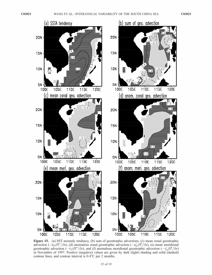
Figure 15. (a) SST anomaly tendency, (b) sum of geostrophic advections, (c) mean zonal geostrophicadvection (��uG@T
0=@x), (d) anomalous zonal geostrophic advection (�u0G@�T=@x), (e) mean meridional
geostrophic advection (��vG@T 0=@y), and (f) anomalous meridional geostrophic advection (�v0G@�T=@y)
in November of 1997. Positive (negative) values are given by dark (light) shading and solid (dashed)contour lines, and contour interval is 0.4�C per 2 months.
C03023 WANG ET AL.: INTERANNUAL VARIABILITY OF THE SOUTH CHINA SEA
15 of 19
C03023
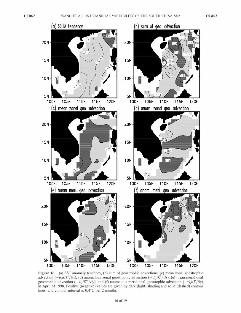
Figure 16. (a) SST anomaly tendency, (b) sum of geostrophic advections, (c) mean zonal geostrophicadvection (��uG@T
0=@x), (d) anomalous zonal geostrophic advection (�u0G@�T=@x), (e) mean meridionalgeostrophic advection (��vG@T 0=@y), and (f) anomalous meridional geostrophic advection (�v0G@�T=@y)in April of 1998. Positive (negative) values are given by dark (light) shading and solid (dashed) contourlines, and contour interval is 0.4�C per 2 months.
C03023 WANG ET AL.: INTERANNUAL VARIABILITY OF THE SOUTH CHINA SEA
16 of 19
C03023
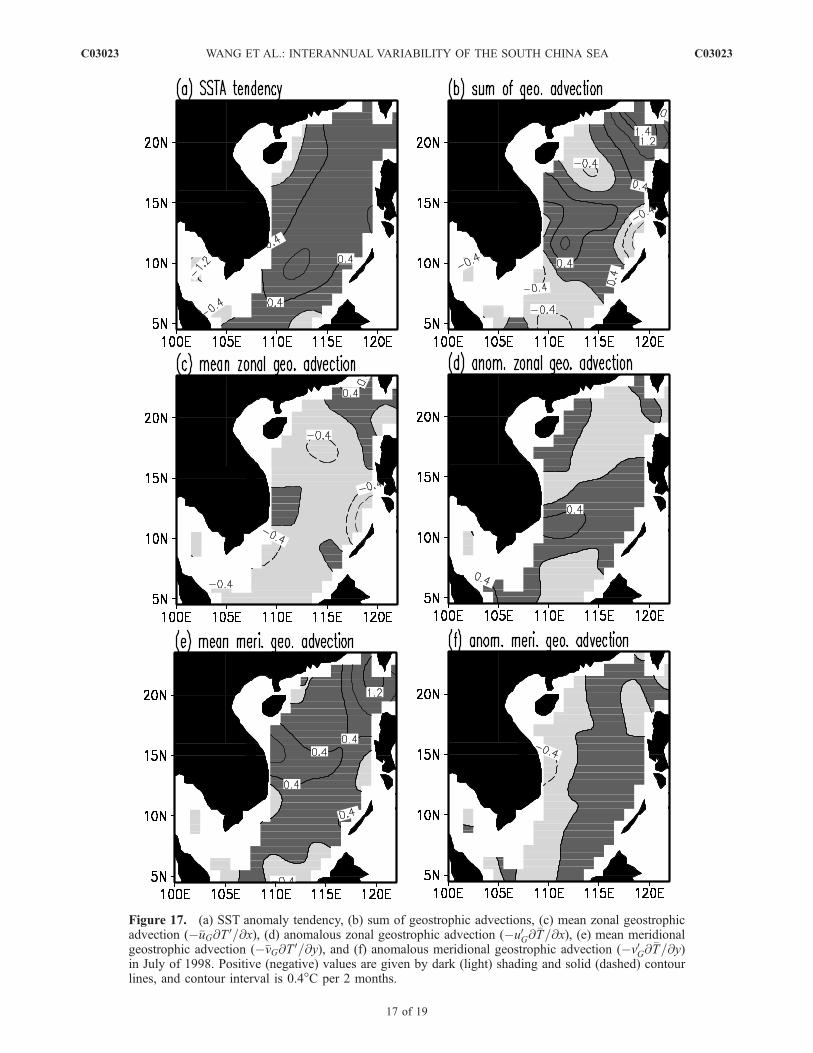
Figure 17. (a) SST anomaly tendency, (b) sum of geostrophic advections, (c) mean zonal geostrophicadvection (��uG@T
0=@x), (d) anomalous zonal geostrophic advection (�u0G@�T=@x), (e) mean meridional
geostrophic advection (��vG@T 0=@y), and (f) anomalous meridional geostrophic advection (�v0G@�T=@y)
in July of 1998. Positive (negative) values are given by dark (light) shading and solid (dashed) contourlines, and contour interval is 0.4�C per 2 months.
C03023 WANG ET AL.: INTERANNUAL VARIABILITY OF THE SOUTH CHINA SEA
17 of 19
C03023
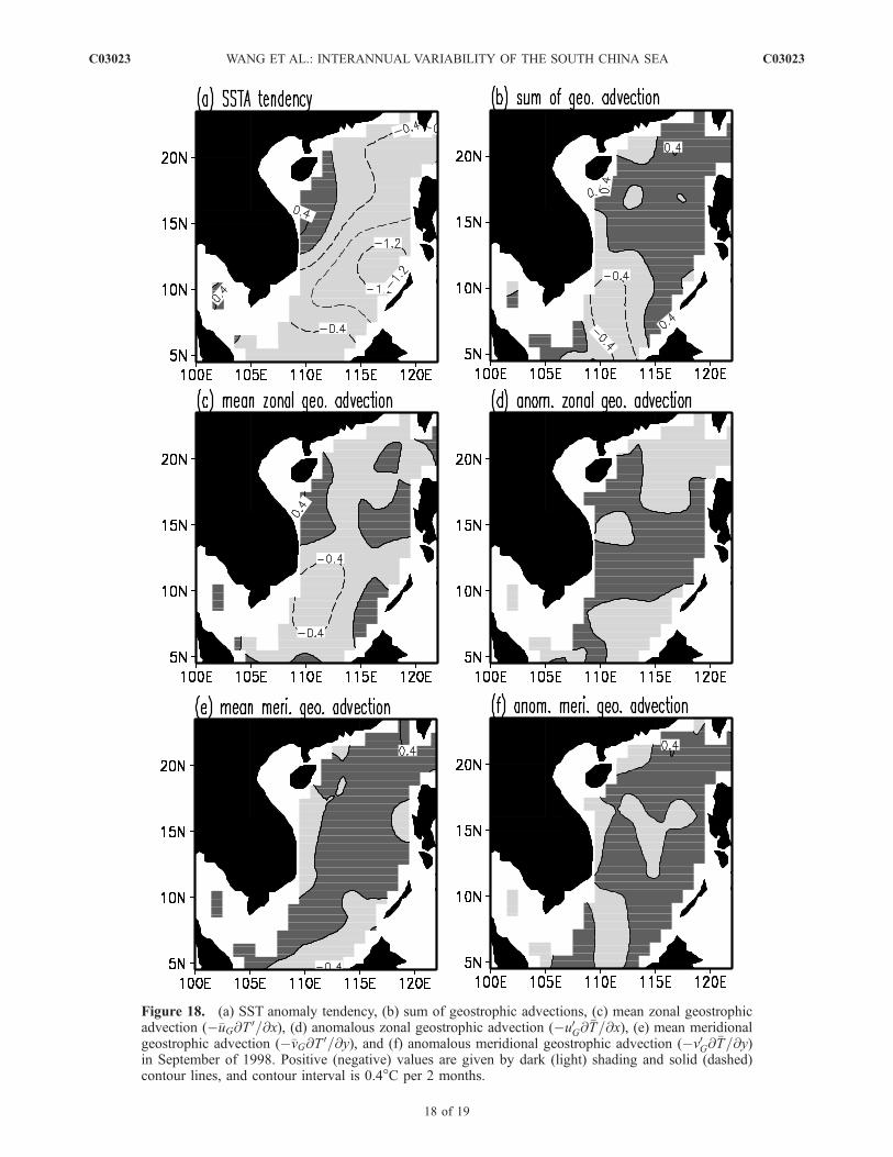
Figure 18. (a) SST anomaly tendency, (b) sum of geostrophic advections, (c) mean zonal geostrophicadvection (��uG@T
0=@x), (d) anomalous zonal geostrophic advection (�u0G@�T=@x), (e) mean meridional
geostrophic advection (��vG@T 0=@y), and (f) anomalous meridional geostrophic advection (�v0G@�T=@y)
in September of 1998. Positive (negative) values are given by dark (light) shading and solid (dashed)contour lines, and contour interval is 0.4�C per 2 months.
C03023 WANG ET AL.: INTERANNUAL VARIABILITY OF THE SOUTH CHINA SEA
18 of 19
C03023
gradient, produce a cooling effect for the SCS as shown inFigure 9d. During April [+1] the mean and anomalousgeostrophic currents over the SCS are northeastward andsouthwestward, respectively. These geostrophic currentsalso help cool the SCS after the first peak of SST anomalies.[35] The SCS SST anomalies peak again in August [+1]
and then decay. The negative values of the surface heat fluxand Ekman heat advections and the smallness of anomalousentrainment heat flux cannot explain the second peak of theSCS SST anomalies. Our analyses show that the meanmeridional geostrophic heat advection is mainly responsiblefor the second peak. The mean geostrophic current of theSCS in the summer is northeastward in response to thesouthwest monsoon. The mean northward current, associ-ated with a southward anomalous SST gradient, results in awarming condition in the SCS as shown in Figure 17e.After the second peak, the latent heat flux anomalies,mainly attributed to the anomalous air-sea difference inspecific humidity, cool the SCS. It is worth to note that themean northeastward geostrophic current also helps cool thesouthern SCS in September [+1].[36] The anomalous entrainment heat flux is always
positive over various stages of the SCS SST anomalyevolution. This occurs because the anomalous Ekmanpumping velocity over the SCS is always downward fol-lowing El Nino events (Figure 6). The downward anoma-lous Ekman pumping and the positive mean verticaltemperature gradient produce a warming trend in the SCS.However, the amplitude of the anomalous entrainment heatflux is smaller than other terms in the SST equation, andthus it plays a secondary role in the SCS SST anomalies.[37] This paper mainly focuses on the SCS SST anoma-
lies associated with the warm phase (El Nino) of ENSO. Anatural question to be asked is: How do the SCS SSTanomalies vary during the cold phase (La Nina) of ENSO?Our analyses show that the double-peak evolution of theSCS SST anomalies following La Nina events in the Pacificis not a common feature. Only in the 1964–1965 and1975–1976 La Nina events does the SCS show two coldpeaks of the SST anomalies (two peaks occur in the winterof the La Nina year and the subsequent spring of the LaNina year, respectively). For some La Nina events, the SCSdoes not even show cold SST anomalies. These imply thatthe response of the SCS SST anomalies to El Nino and LaNina is not symmetric. However, for the cases that the SCSdoes show cold SST anomalies following La Nina events,the net surface heat flux anomalies play a major role.Finally, we would like to caution that the heat budgetcalculations in this paper are based on multiple observa-tional data sets described in Section 2, and thus the roles ofvarious terms in the SCS SST anomalies may depend uponthese data sets. Nevertheless, these data sets are probablythe best long-term data available for us to study interannualvariability over the SCS.
[38] Acknowledgments. We thank S.-P. Xie and T. Qu for discus-sions during the early stage of the work. Comments by reviewers and theeditor are appreciated. The work was done when W.W. and D.W. visited theNational Oceanic and Atmospheric Administration (NOAA) AtlanticOceanographic and Meteorological Laboratory (AOML). This work issupported by a grant from NOAA Office of Global Programs, the base
funding of NOAA/AOML, National Natural Science Foundation of China(grants 40476009, 40306003, and 40136010), National Basic ResearchProgram of China (grant 2005CB422301), and the funding of the K. C.Wong Education Foundation. The findings and conclusions in this reportare those of the author(s) and do not necessarily represent the views of thefunding agency.
ReferencesAlexander, M. A., et al. (2002), The atmospheric bridge: The influenceof ENSO teleconnections on air-sea interaction over the global oceans,J. Clim., 15, 2205–2231.
da Silva, A., C. Young-Molling, and S. Levitus (1994), Atlas of SurfaceMarine Data 1994, vol. 3, Anomalies of Heat and Momentum Fluxes,NOAA Atlas NESDIS, vol. 8, NOAA, Silver Spring, Md.
Ducet, N., P. Y. Le Traon, and G. Reverdin (2000), Global high-resolutionmapping of ocean circulation from TOPEX/Poseidon and WRS-1 and -2,J. Geophys. Res., 105, 19,477–19,498.
Fung, I. Y., D. E. Harrison, and A. A. Lacis (1984), On the variability of thenet longwave radiation at the ocean surface, Rev. Geophys., 22, 177–193.
Klein, S. A., B. J. Soden, and N. C. Lau (1999), Remote sea surfacetemperature variations during ENSO: Evidence for a tropical Atmo-spheric bridge, J. Clim., 12, 917–932.
Levitus, S., and T. P. Boyer (1994), World Ocean Atlas 1994, vol. 4,Temperature, NOAA Atlas NESDIS, vol. 4, 129 pp., NOAA, SilverSpring, Md.
Liu, Q., X. Jiang, S.-P. Xie, and W. T. Liu (2004), A gap in the Indo-Pacificwarm pool over the South China Sea in boreal winter: Seasonal devel-opment and interannual variability, J. Geophys. Res., 109, C07012,doi:10.1029/2003JC002179.
Qu, T. (2001), Role of ocean dynamics in determining the mean seasonalcycle of the South China Sea surface temperature, J. Geophys. Res., 106,6943–6955.
Qu, T., et al. (2004), Can Luzon strait transport play a role in conveying theimpact of ENSO to the South China Sea?, J. Clim., 17, 3644–3657.
Wang, C. (2002), Atmospheric circulation cells associated with theEl Nino–Southern Oscillation, J. Clim., 15, 399–419.
Wang, C. (2005), ENSO, Atlantic climate variability, and the Walker andHadley circulations, in The Hadley Circulation: Past, Present andFuture, edited by H. F. Diaz and R. S. Bradley, pp. 173–202, Springer,New York.
Wang, C., R. H. Weisberg, and J. I. Virmani (1999), Western Pacificinterannual variability associated with the El Nino–Southern Oscilla-tion, J. Geophys. Res., 104, 5131–5149.
Wang, C., S.-P. Xie, and J. A. Carton (2004), A global survey of ocean-atmosphere interaction and climate variability, in Earth’s Climate: TheOcean-Atmosphere Interaction, Geophys. Monogr. Ser., vol. 147, editedby C. Wang, et al., pp. 1–19, AGU, Washington, D. C.
Wang, D., Q. Xie, Y. Du, W. Q. Wang, and J. Chen (2002), The 1997–1998warm event in the South China Sea, Chin. Sci. Bull., 47, 1221–1227.
Wang, Q., Q. Liu, R. Hu, and Q. Xie (2002), A possible role of the SouthChina Sea in ENSO cycle, Acta Oceanol. Sin., 21, 217–226.
Wang, W., D. Wang, and Y. Qi (2000), Large-scale characteristics of inter-annual variability of sea surface temperature in the South China Sea, ActaOceanol. Sin., 22, 8–16.
Weisberg, R. H., and C. Wang (1997), Awestern Pacific oscillator paradigmfor the El Nino–Southern Oscillation, Geophys. Res. Lett., 24, 779–782.
Woodruff, S. D., R. J. Slutz, R. L. Jenne, and P. M. Steurer (1987), Acomprehensive ocean-atmosphere data set, Bull. Am. Meteorol. Soc.,68, 521–527.
Xie, S.-P., Q. Xie, D. Wang, and W. T. Liu (2003), Summer upwelling inthe South China Sea and its role in regional climate variations, J. Geo-phys. Res., 108(C8), 3261, doi:10.1029/2003JC001867.
Yang, H., Q. Liu, Z. Liu, D. Wang, and X. Liu (2002), A general circula-tion model study of the dynamics of the upper ocean circulation of theSouth China Sea, J. Geophys. Res., 107(C7), 3085, doi:10.1029/2001JC001084.
�����������������������C. Wang, Atlantic Oceanographic and Meteorological Laboratory,
Physical Oceanography Division, NOAA, 4301 Rickenbacker Causeway,Miami, FL 33149, USA. ([email protected])D. Wang and W. Wang, Key Laboratory of Tropical Marine Environ-
mental Dynamics, South China Sea Institute of Oceanology, ChineseAcademy of Sciences, 164 West Xingang Rd., Guangzhou 510301, China.Q. Wang, Department of Meteorology, Physical Oceanography Labora-
tory, Ocean University of China, 5 Yushan Road, Qingdao 266003 China.
C03023 WANG ET AL.: INTERANNUAL VARIABILITY OF THE SOUTH CHINA SEA
19 of 19
C03023