Embed Size (px)
Citation preview
1
Seasonal to interannual variability of Chlorophyll-a and sea surface 1
temperature in the Yellow Sea using MODIS satellite datasets 2
Chunli Liu,1 Qiwei Sun,
2,3 Sufen Wang,
2 Qianguo Xing,
4 3
Lixin Zhu,1 Zhenling Liang
1 4
5
1Marine college, Shandong University (Weihai), 264209, China 6
2The State Key Laboratory of Tropical Oceanography, South China Sea Institute of 7
Oceanology, Chinese Academy of Sciences, 510301, China 8
3University of Chinese Academy of Sciences, 100049, China 9
4Yantai Institute of Coastal Zone Research, Chinese Academy of Sciences, 264003, 10
China 11
12
13
Correspondence to: Zhenlin Liang ([email protected]) 14
15
Ocean Sci. Discuss., doi:10.5194/os-2017-11, 2017Manuscript under review for journal Ocean Sci.Discussion started: 28 April 2017c© Author(s) 2017. CC-BY 3.0 License.
2
Abstract: The spatial and temporal variability of Chlorophyll-a concentration (CHL) 16
and sea surface temperature (SST) in the Yellow Sea (YS) were examined using 17
Empirical Orthogonal Function (EOF) analysis, which was based on the monthly, 18
cloud-free Data INterpolating Empirical Orthogonal Function (DINEOF) 19
reconstruction datasets for 2003–2015. The variability and oscillation periods on an 20
inter-annual timescale were also confirmed using the Morlet wavelet transform and 21
wavelet coherence analyses. At a seasonal time scale, the CHL EOF1 mode was 22
dominated by a seasonal cycle of a spring and a fall bloom, with a spatial distribution 23
that was modified by the strong mixing of the water column of the Yellow Sea Cold 24
Warm Mass (YSCWM) that facilitated nutrient delivery from the ocean bottom. The 25
EOF2 mode was likely associated with a winter bloom in the southern region, where 26
it was affected by the Yellow Sea Warm Current (YSWC) that moved from southeast 27
to north in winter. The SST EOF1 explained 99 % of the variance in total variabilities, 28
which was dominated by an obvious seasonal cycle (in response to net surface heat 29
flux) that was inversely proportional to the water depth. At the inter-annual scale, the 30
wavelet power spectrum and global power spectrum of CHL and SST showed 31
significant similar periods of variations. The dominant periods for both spectra were 32
2–4 years during 2003–2015. A significant negative cross-correlation existed between 33
CHL and SST, with the largest correlation coefficient at time lags of 4 months. The 34
wavelet coherence further identified a negative relationship that was significant 35
statistically between CHL and SST during 2008–2015, with periods of 1.5–3 years. 36
These results provided insight into how CHL might vary with SST in the future. 37
Ocean Sci. Discuss., doi:10.5194/os-2017-11, 2017Manuscript under review for journal Ocean Sci.Discussion started: 28 April 2017c© Author(s) 2017. CC-BY 3.0 License.

3
Key words: Empirical orthogonal function analysis; Continuous wavelet transform; 38
Wavelet coherency analysis; Sea surface temperature; Chlorophyll-a 39
40
1. Introduction 41
Chlorophyll-a concentrations (CHL), as an index of phytoplankton pigment, are 42
considered an important indicator of eutrophication in marine ecosystems, which is a 43
process that may affect human life (Smith, 2006; Werdell et al., 2009). Additionally, 44
it can be used to analyze the comprehensive dynamics of phytoplankton biomass 45
(Muller-Karger et al., 2005). On the other hand, sea surface temperature (SST) 46
anomalies indicate stratification of the water column, which is related closely to light 47
and to nutrient loads of CHL (He et al., 2010). Certain studies have reported the 48
spatio-temporal variability and relationship between CHL and SST (Gregg et al., 2005; 49
Behrenfeld et al., 2006; Boyce et al., 2010). In the open ocean, Wilson and Coles 50
(2005) analyzed global scale relationships between CHL and the monthly SST. 51
Similarly, the spatio-temporal variability of regional CHL and SST in the South 52
Atlantic Bight and the Mediterranean Sea have been investigated using long-term 53
satellite datasets (Miles and He, 2010; Volpe et al., 2012). Gao et al. (2013) examined 54
the spatio-temporal distribution of CHL that was associated with SST in the western 55
South China Sea using the Sea-viewing Wide Field-of-View Sensor (SeaWiFS) and 56
National Oceanic and Atmospheric Administration Advanced Very High Resolution 57
Radiometer (AVHRR) data. For coastal waters, Li and He (2014) examined 58
spatio-temporal distribution of CHL that was associated with SST in the Gulf of 59
Ocean Sci. Discuss., doi:10.5194/os-2017-11, 2017Manuscript under review for journal Ocean Sci.Discussion started: 28 April 2017c© Author(s) 2017. CC-BY 3.0 License.

4
Maine (GOM) using daily MODIS data. Moradi and Kabiri (2015) examined the 60
spatio-temporal variability of CHL and SST in the Persian Gulf using MODIS 61
Level-2 products. These studies found region-specific relationships between 62
climate-driven SST and CHL. These findings also indicated that knowledge of the 63
spatio-temporal variability in CHL and SST can assist scientists in developing a more 64
comprehensive perspective of biological and physical oceanography of marine 65
ecosystems in the global scale. 66
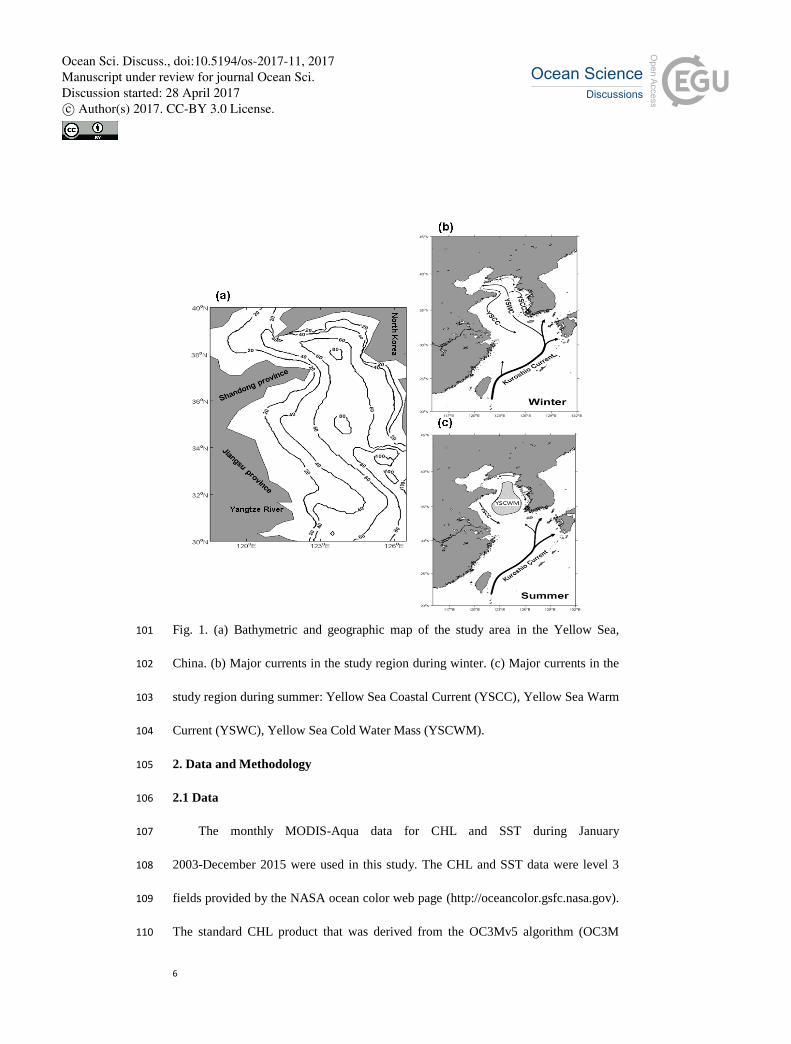
The Yellow Sea (YS) has an average water depth of only 44 m, and it is marginal 67
seas surrounded by China, and Korea (Fig. 1a). It responds quickly to atmospheric 68
climate change and, in turn, the YS influences local climate variability as a result of 69
the air-sea feedback process. The Yellow Sea Warm Current (YSWC) moves from 70
southeast to north in winter (Fig.1b) (Teague and Jacobs, 2000; Lie et al., 2009; Yu et 71
al., 2010), and the Yellow Sea Cold Water Mass (YSCWM; 122–125° E, 33–37° N) 72
is entrenched at the bottom in summer (Fig. 1c) (Zhang et al., 2008). These water 73
masses represent the two most important physical oceanographic features in the YS. 74
In addition, a southward coastal flow is present in winter along the eastern and 75
western sides of the YS, which corresponds to the northward YSWC in the central sea 76
area (Wei et al., 2016; Xu et al., 2016). These features affect the physical properties, 77
water mass and circulation in the YS, and they are complicated both spatially and 78
temporally (Chu et al., 2005). 79
To date, the importance of SST variability and the associated features such as 80
thermal or tidal fronts, coastal waters, and currents in the YS have been addressed by 81
Ocean Sci. Discuss., doi:10.5194/os-2017-11, 2017Manuscript under review for journal Ocean Sci.Discussion started: 28 April 2017c© Author(s) 2017. CC-BY 3.0 License.

5
numerous satellite-based studies (Tseng et al., 2000; Lin et al., 2005; Wei et al., 2010; 82
Yeh and Kim, 2010; Shi and Wang, 2012), and the long term CHL trends and 83
seasonal variations have been studied as well (Shi and Wang, 2012; Yamaguchi, et al., 84
2012; Liu and Wang, 2013). In recent years, warming signals of SST in the YS were 85
reported by Yeh and Kim (2010) and Park et al. (2015), but few researchers have paid 86
attention to how has the increasing SST affected the spatio-temporal pattern of CHL 87
in the YS? What is the region-specific relationship between climate-driven SST and 88
CHL? 89
To answer these questions, we combined remote sensing datasets and statistical 90
analysis to investigate the patterns of variability of CHL and SST over seasonal and 91
inter-annual periods at temporal scales during 2003–2015 in the YS. The present work 92
provides a comprehensive description of the phytoplankton biomass and the physical 93
conditions using 13 years of satellite-derived datasets. The objectives of the study 94
were (i) to identify the seasonal spatial and temporal patterns of CHL and SST with 95
the empirical orthogonal function (EOF) statistical model in the YS, (ii) to investigate 96
the inter-annual trends of CHL and SST in a long-term time series with the continuous 97
wavelet transform (CWT) analysis, and (iii) to explore the temporal correlations 98
between CHL and SST using wavelet coherency analysis at a regional scale. 99
100
Ocean Sci. Discuss., doi:10.5194/os-2017-11, 2017Manuscript under review for journal Ocean Sci.Discussion started: 28 April 2017c© Author(s) 2017. CC-BY 3.0 License.
6
Fig. 1. (a) Bathymetric and geographic map of the study area in the Yellow Sea, 101
China. (b) Major currents in the study region during winter. (c) Major currents in the 102
study region during summer: Yellow Sea Coastal Current (YSCC), Yellow Sea Warm 103
Current (YSWC), Yellow Sea Cold Water Mass (YSCWM). 104
2. Data and Methodology 105
2.1 Data 106
The monthly MODIS-Aqua data for CHL and SST during January 107
2003-December 2015 were used in this study. The CHL and SST data were level 3 108
fields provided by the NASA ocean color web page (http://oceancolor.gsfc.nasa.gov). 109
The standard CHL product that was derived from the OC3Mv5 algorithm (OC3M 110
Ocean Sci. Discuss., doi:10.5194/os-2017-11, 2017Manuscript under review for journal Ocean Sci.Discussion started: 28 April 2017c© Author(s) 2017. CC-BY 3.0 License.
7
updated version after the 2009 reprocessing) and the daytime SST 11 μm product 111
(which uses the 11 and 12 μm bands) were obtained. The level 3 product was 112
collected in a 4 km spatial resolution from 30–40° N in latitude and 118–126° E in 113
longitude for the YS region. 114
2.2. Methodology 115
2.2.1 DINEOF 116
Due to the cloud coverage of the MODIS images over the YS, MODIS pixel 117
values were missing for some months. The EOF and wavelet analyses generally 118
require a complete time series of input maps without data voids. Therefore, a method 119
to reconstruct missing data based on the Data Interpolating Empirical Orthogonal 120
Functions (DINEOF) decomposition was applied to obtain complete CHL and SST 121
data (Beckers and Rixen, 2003; Beckers et al. 2006). It is a self-consistent, 122
parameter-free technique for gappy data reconstruction. Recently, DINEOF has been 123
used widely to reconstruct SST (Miles and He, 2010; Huynh et al., 2016), CHL and 124
winds (Miles and He, 2010; Volpe et al., 2012; Liu and Wang, 2013; Liu et al., 2014), 125
total suspended matter (Sirjacobs et al., 2011; Alvera-Azcarate et al., 2015), and sea 126
surface salinity (Alvera-Azcarate et al., 2016). This technique presents some 127
advantages over more classical approaches (such as optimal interpolation), especially 128
when working on CHL and SST datasets (Miles and He, 2010; Volpe et al., 2012). 129
CHL and SST are characterized by different scales of variability in coastal or open 130
ocean areas. This method identifies dominant spatial and temporal patterns in CHL 131
and SST datasets, and it fills in missing data. Thus, DINEOF was applied to 132
Ocean Sci. Discuss., doi:10.5194/os-2017-11, 2017Manuscript under review for journal Ocean Sci.Discussion started: 28 April 2017c© Author(s) 2017. CC-BY 3.0 License.

8
reconstruct the missing CHL and SST data in this study. Because the satellite CHL 133
values spanned three orders of magnitude and CHL retrievals are often distributed 134
log-normally (Campbell, 1995), raw data were log-transformed prior to reconstruction 135
to homogenize the variance and to yield a near-normal distribution (Fig. 2). These 136
images show clearly the utility of the DINEOF method in reconstructing monthly, 137
high-resolution imagery from datasets with large amounts of cloud cover. For 138
example, in the CHL, DINEOF gives a low concentration of CHL in the southeast 139
regions of the YS (Fig. 2b). 140
141
Fig. 2. The spatial pattern of CHL in Jan 2011. (a) cloud-covered and (b) DINEOF 142
reconstructed CHL; the spatial pattern of SST in Jan 2011. (c) cloud-covered and (d) 143
DINEOF reconstructed SST. 144
Ocean Sci. Discuss., doi:10.5194/os-2017-11, 2017Manuscript under review for journal Ocean Sci.Discussion started: 28 April 2017c© Author(s) 2017. CC-BY 3.0 License.

9
2.2.2 Empirical Orthogonal Function (EOF) analysis 145
After DINEOF reconstruction, cloud free CHL values were log-transformed 146
before we included them in figures and before statistical analysis. In Section 4, to 147
better discern the spatial heterogeneity and the degree of coherence and temporal 148
evolution of the CHL and SST fields, a traditional EOF analysis was applied further 149
to the monthly, cloud-free DINEOF CHL and SST datasets, which is an approach that 150
is also used widely in other disciplines (Hu and Si, 2016a). Each data set was 151
organized in an M×N matrix, where M and N represented the spatial and temporal 152
elements, respectively. Taking CHL for instance, the matrix 𝐼(𝑥, 𝑡) can be 153
represented by 𝐼(𝑥, 𝑡) = ∑ 𝑎𝑛(𝑡)𝐹𝑛(𝑥)𝑁𝑛=1 , where 𝑎𝑛(𝑡) are the temporal evolution 154
functions and 𝐹𝑛(𝑥, 𝑦) are the spatial eigen-functions for each EOF mode. Prior to 155
EOF analysis, the temporal means of each pixel were removed from the original data 156
using: 𝐼′(𝑥, 𝑡) = 𝐼(𝑥, 𝑡) − 1/𝑁 ∑ 𝐼(𝑥, 𝑡𝑗)𝑁𝑗=1 , where 𝐼′(𝑥, 𝑡) are the resulting residuals 157
(anomalies). The first two modes were decomposed to analyze the major variability in 158
CHL and SST. 159
To assess the significance of the EOF modes, we followed the methods 160
described by North et al. (1982). The error produced in a given EOF (ej) was 161
calculated as: 𝑒𝑗 = 𝜆𝑗 ( 2/𝑛)0.5, where λ is the eigenvalue of that EOF, and n is the 162
degrees of freedom. When the difference between neighboring eigenvalues satisfied 163
𝜆𝑗 − 𝜆𝑗+1 ≥ 𝑒𝑗, then the EOF modes represented by these two eigenvalues were 164
significant statistically. 165
2.2.3 The continuous wavelet transform (CWT) 166
Ocean Sci. Discuss., doi:10.5194/os-2017-11, 2017Manuscript under review for journal Ocean Sci.Discussion started: 28 April 2017c© Author(s) 2017. CC-BY 3.0 License.

10
The continuous wavelet transform (CWT) was used to determine the 167
inter-annual scales of variability and the oscillation periods of DINEOF CHL and SST. 168
Prior to the CWT analysis, the seasonal variation of each pixel was removed from the 169
original data. The CWT is a tool for decomposing the non-stationary time series at 170
different spatial or time scales into the time-frequency space by translation of the 171
mother wavelet and by analyzing localized variations of power (Messié and Chavez, 172
2011). The mother wavelets used in this study were the “Morlet” wavelets, which is 173
used commonly in geophysics, because it provides a good balance between time and 174
frequency localization (Grinsted et al., 2004; Hu and Si, 2016b; She et al., 2016). The 175
CWT can localize the signal in both the time and frequency domains, but the classical 176
Fourier transform was able to localize the signal only in the frequency domain with no 177
localization in time (Olita et al., 2011). In addition, cross-correlation functions 178
(Venables and Ripley, 2002) were used to determine the degree of temporal 179
correspondence between the CHL and SST time series datasets, after we removed the 180
seasonal variations. Then, the wavelet coherence was used to show the local 181
correlation between CHL and SST in time-frequency space (Ng and Chan, 2012) that 182
was based on the cross-correlation result. We used the wavelet software provided by 183
Grinsted et al. (2004) (http://noc.ac.uk/usingscience/cross 184
wavelet-wavelet-coherence). 185
3. Results 186
3.1 Monthly Climatology of CHL and SST 187
The CHL monthly means during 2003–2015 followed a similar pattern from 188
Ocean Sci. Discuss., doi:10.5194/os-2017-11, 2017Manuscript under review for journal Ocean Sci.Discussion started: 28 April 2017c© Author(s) 2017. CC-BY 3.0 License.
11
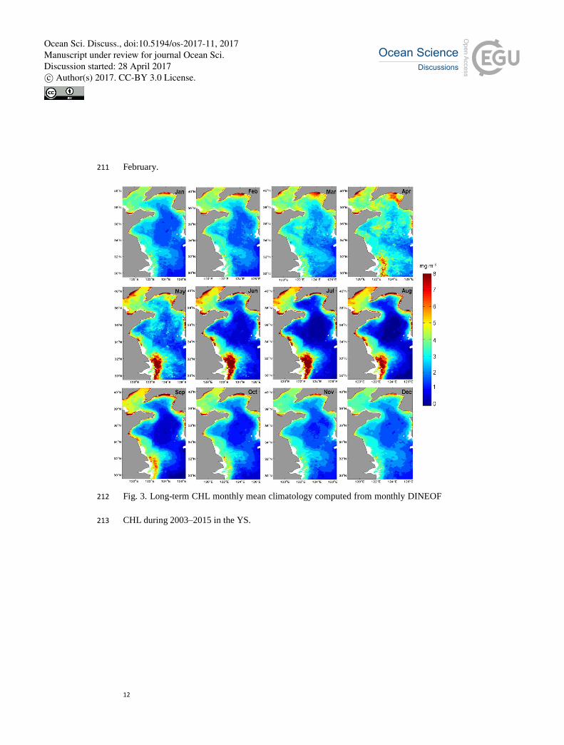
month to month, with more CHL in the shallow coastal waters and a decreased in the 189
seaward direction (Fig. 3). Although the maximum CHL appeared to be fairly 190
consistent seasonally, the spatial extent of blooms had significant seasonal 191
fluctuations. Monthly mean imagery showed the largest spatial coverage of CHL in 192
YS was in spring and the smallest coverage was in summer. The CHL in coastal 193
waters was relatively high in spring during every year. Some portions of 194
phytoplankton blooms occurred only in subsurface waters, which made it impossible 195
to see using satellite imagery. Overall, the CHL was the greatest in coastal waters in 196
spring or in regions with greater diluted water, such as near the Yangtze River, where 197
the CHL was characterized by a long-lasting summer CHL maximum that started in 198
April and ended in September. 199
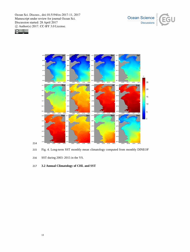
The seasonal cycle was more evident in the SST field (Fig. 4). SST showed a 200
sinusoidal seasonal cycle, with a persistent, seasonal, warming trend from winter 201
(February) to summer (August). The SST in the YS during December–April were 202
below 12 °C, increased to 15 °C in May, reached a maximum above 25 °C in August, 203
and then decreased again in September–October. From December to May, there was a 204
drastic temperature difference between northern waters and southern waters, but the 205
SST during summer months was nearly uniform over the entire YS. Spatially, 206
isotherms were generally parallel to the isobaths. There was a clear temperature 207
contrast between coastal waters and offshore waters in winter and spring. Similarly, 208
the thermal front in southeast waters was more visible during winter and spring. The 209
thermal difference reached as high as ~ 4 °C between northern and southern regions in 210
Ocean Sci. Discuss., doi:10.5194/os-2017-11, 2017Manuscript under review for journal Ocean Sci.Discussion started: 28 April 2017c© Author(s) 2017. CC-BY 3.0 License.
12
February. 211
Fig. 3. Long-term CHL monthly mean climatology computed from monthly DINEOF 212
CHL during 2003–2015 in the YS. 213
Ocean Sci. Discuss., doi:10.5194/os-2017-11, 2017Manuscript under review for journal Ocean Sci.Discussion started: 28 April 2017c© Author(s) 2017. CC-BY 3.0 License.
13
214
Fig. 4. Long-term SST monthly mean climatology computed from monthly DINEOF 215
SST during 2003–2015 in the YS. 216
3.2 Annual Climatology of CHL and SST 217
Ocean Sci. Discuss., doi:10.5194/os-2017-11, 2017Manuscript under review for journal Ocean Sci.Discussion started: 28 April 2017c© Author(s) 2017. CC-BY 3.0 License.

14
Spatial variation in the annual mean CHL during 2003–2015 resembled that of 218
the monthly mean CHL (Fig. 5). CHL was relatively low in offshore waters in the YS 219
and it was higher in the narrow band along the coast, where CHL was stable, except 220
for areas near the Yangtze River. Inter-annual variation of CHL was relatively subtle 221
in the YS, and mean annual values ranged from 2.65 to 3.28 mg m–3
. The maximum 222
CHL occurred in 2011, and the minimum CHL were observed in 2003. In summary, 223
the CHL was stable and revealed the stationary level of CHL in the YS irrespective of 224
monthly or annual cycles. 225
Fig. 5. CHL annual mean climatology computed from monthly DINEOF CHL during 226
2003–2015 in the YS. 227
Ocean Sci. Discuss., doi:10.5194/os-2017-11, 2017Manuscript under review for journal Ocean Sci.Discussion started: 28 April 2017c© Author(s) 2017. CC-BY 3.0 License.

15
228
Fig. 6. SST annual mean climatology computed from monthly DINEOF SST during 229
2003–2015 in the YS. 230
For each year during 2003–2015, the annual isotherms of SST generally ran 231
parallel to the isobaths (Fig. 6). There was a clear temperature contrast between 232
northern and southern waters. Similarly, the thermal front in southeast waters was 233
visible each year. The thermal difference reached as high as ~ 5 °C between northern 234
and southern waters in 2011. Inter-annual variation of the SST was relatively minor, 235
and ranged from 15.17 to 16.88 °C. The maximum SST occurred in 2015, and the 236
minimum SST was in 2011. 237
3.3 Monthly mean and temporal variability of CHL and SST 238
The spatial patterns of CHL and SST concentration were produced by the 239
Ocean Sci. Discuss., doi:10.5194/os-2017-11, 2017Manuscript under review for journal Ocean Sci.Discussion started: 28 April 2017c© Author(s) 2017. CC-BY 3.0 License.

16
temporal means of monthly data during 2003–2015 (Fig. 7a and c) and variability 240
associated with the standard deviations (STD) of monthly mean temporal values (Fig. 241
7b and d). One general evident spatial pattern was that mean CHL showed a sharp 242
decrease from coastal waters to offshore regions (Fig. 7a). In our study, the highest 243
CHL values (~ 6 mg m–3
) and the lowest STD (~ 0.02 mg m–3
) were observed in 244
coastal waters (Fig. 7b) that were adjacent to the mouth of the Yangtze River where 245
the water depth was less than 20 m. Compared with the coastal waters and the sea 246
adjacent to large river mouths, central YS waters had lower CHL, but they displayed 247
greater variability. In these regions, strong water mixing could make more deep-ocean 248
nutrients available for utilization by phytoplankton in some months. The 249
spatially-averaged time series showed clear inter-annual variability that was 250
superimposed on the seasonal spring (April) and fall (August) blooms (Fig. 7e). A 251
noticeable scenario was the increasing trend in CHL of ~ 0.03 mg m–3
year–1
252
throughout the YS during 2003–2015; this phenomenon would require more 253
observations of subsurface nutrients to understand the underlying mechanisms. 254
The spatial distribution of the 13-year averaged SST in the YS showed the mean 255
SST with a smooth transition from colder water along the coast to warmer water in 256
offshore areas (Fig. 7c). Similarly, SST in the northern YS was colder compared to 257
that in the southern YS. In contrast, the STD calculated from the 13-year time series 258
of SST also revealed a high spatial distinction between the northern and southern 259
regions (Fig. 7d). In the northern region, the STD reached its highest values in excess 260
of 8 °C, in contrast to the STD of the southeastern YSWC region, which were 261
Ocean Sci. Discuss., doi:10.5194/os-2017-11, 2017Manuscript under review for journal Ocean Sci.Discussion started: 28 April 2017c© Author(s) 2017. CC-BY 3.0 License.

17
relatively small. Similarly, the zonal distribution of the variability demonstrated that 262
the western region contained a much higher variability greater than 6.5 °C, which 263
contrasted with the relatively small variability in the eastern region. The spatial mean 264
of SST anomalies was superimposed by synoptic and inter-annual variability signals, 265
which showed a positive trend of ~ 0.02 °C year–1
during 2003–2015 (Fig. 7f). 266
Fig. 7. Long-term temporal mean and standard deviation maps of DINEOF CHL 267
during 2003–2015 in the YS. (a) spatial pattern of temporal mean and (b) standard 268
deviation map. Long-term temporal mean and standard deviation maps of DINEOF 269
SST during 2003–2015 in the YS; (c) spatial pattern of temporal mean and (d) 270
Ocean Sci. Discuss., doi:10.5194/os-2017-11, 2017Manuscript under review for journal Ocean Sci.Discussion started: 28 April 2017c© Author(s) 2017. CC-BY 3.0 License.

18
standard deviation map. Time series of mean anomalies for DINEOF values during 271
2003–2015 in the YS. The blue lines are least-square linear fits; (e) CHL anomaly and 272
(f) SST anomaly. 273
4. Discussion 274
4.1 Modes of the variability in CHL and SST 275
4.1.1 The dominant CHL EOF mode 276
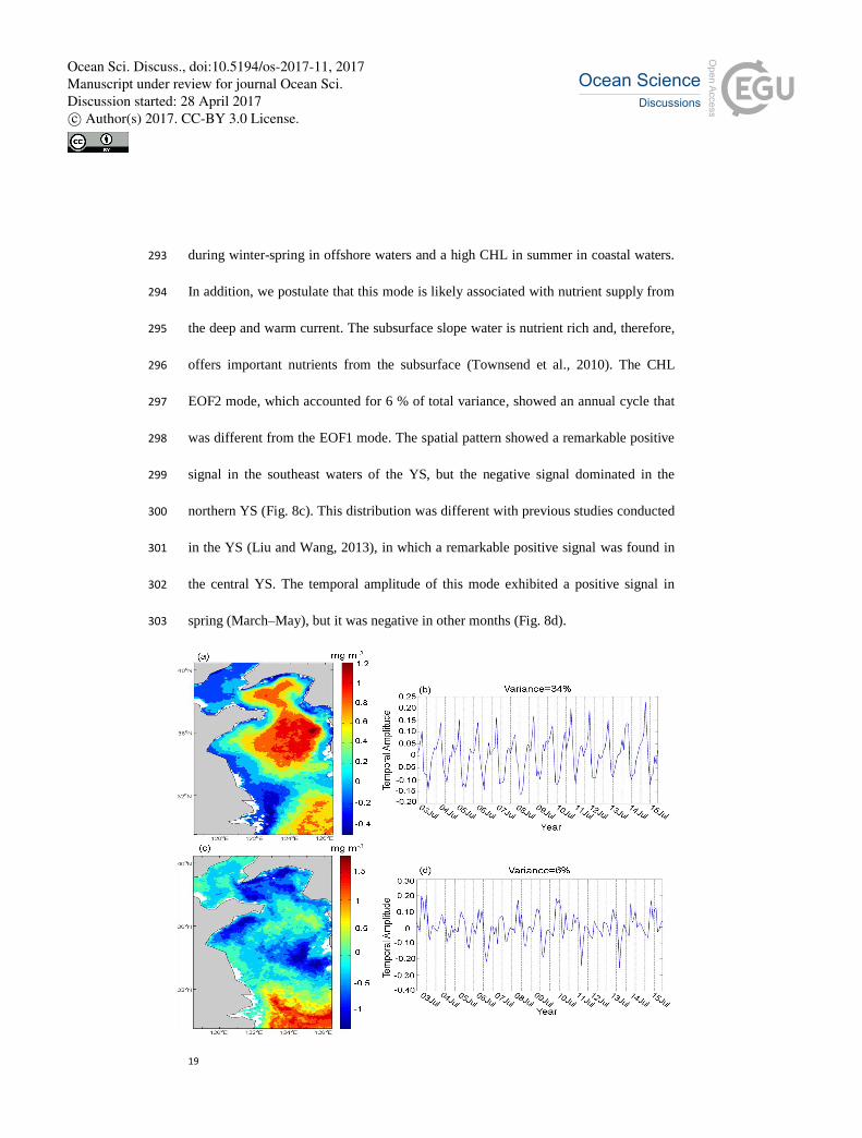
The first EOF (EOF1) and second EOF (EOF2) modes accounted for 40 % of 277
the total CHL variability in this study (Fig. 8), which are similar to those observed in 278
previous studies on the regional and global CHL (Messié and Radenac, 2006; Thomas 279
et al., 2012). The CHL EOF1 mode explained 34 % of the total variance. The 280
anomalies were not distributed uniformly throughout the entire study area (Fig. 8a). 281
One of the centers of CHL anomalies was located in an area with the geographical 282
coordinates of about 35–37° N and 122–126° E, which was affected mainly by the 283
YSCWM in the central waters of the YS (Teague and Jacobs, 2000; Lie et al., 2009; 284
Yu et al., 2010). In that location, the stronger mixing of the water column brought the 285
deeper nutrients upward, in turn favoring a phytoplankton bloom (Liu and Wang, 286
2013). Another CHL positive center was in the southeast waters close to the YSWC, 287
which indicated that the EOF1 mode could be explained by the influences of the 288
currents in the YS. As such, EOF1 mode is a good representation of differences in the 289
timing of the blooms. The temporal amplitude showed positive values from winter to 290
spring (November to April) but negative values from summer and autumn (June to 291
October) (Fig. 8b). The result was related to the seasonal cycles, with a high CHL 292
Ocean Sci. Discuss., doi:10.5194/os-2017-11, 2017Manuscript under review for journal Ocean Sci.Discussion started: 28 April 2017c© Author(s) 2017. CC-BY 3.0 License.
19
during winter-spring in offshore waters and a high CHL in summer in coastal waters. 293
In addition, we postulate that this mode is likely associated with nutrient supply from 294
the deep and warm current. The subsurface slope water is nutrient rich and, therefore, 295
offers important nutrients from the subsurface (Townsend et al., 2010). The CHL 296
EOF2 mode, which accounted for 6 % of total variance, showed an annual cycle that 297
was different from the EOF1 mode. The spatial pattern showed a remarkable positive 298
signal in the southeast waters of the YS, but the negative signal dominated in the 299
northern YS (Fig. 8c). This distribution was different with previous studies conducted 300
in the YS (Liu and Wang, 2013), in which a remarkable positive signal was found in 301
the central YS. The temporal amplitude of this mode exhibited a positive signal in 302
spring (March–May), but it was negative in other months (Fig. 8d). 303
c
Ocean Sci. Discuss., doi:10.5194/os-2017-11, 2017Manuscript under review for journal Ocean Sci.Discussion started: 28 April 2017c© Author(s) 2017. CC-BY 3.0 License.
20
Fig. 8. The first two prominent EOF modes for CHL variability using DINEOF CHL 304
anomaly data during 2003–2015 in the YS. (a) spatial pattern and (b) temporal 305
amplitude from EOF1 mode; (c) spatial pattern and (d) temporal amplitude from 306
EOF2 mode. 307
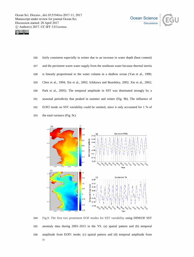
4.1.2 The dominant SST EOF mode 308
The SST EOF1 mode accounted for 99 % of the total variance (Fig. 9a). SST 309
anomalies in the EOF1 mode for the entire study area were all positive, but they were 310
not distributed uniformly throughout the entire study area. This indicated that SST 311
exhibited a positive trend, which was consistent with the pattern that was depicted in 312
Fig. 7f. Similar trends were observed by Liu and Wang (2013) and Park (2015) in 313
their analysis of YS SSTs during the period 1997–2011 and 1981–2009, respectively. 314
As a result of water depth, the SST spatial EOF1 was highly correlated with the 315
distribution of water depth in the YS. The magnitude of variability of EOF1 in 316
shallow water was larger compared to that in the slope region, which suggested an 317
inverse relationship between the general pattern of CHL and bathymetry (O'Reilly et 318
al., 1987). The strong match between the mean CHL and SST patterns throughout the 319
entire YS region can be explained in terms of lower primary production levels that 320
corresponded to stronger stratification of the water column (Behrenfeld et al., 2006; 321
Doney, 2006) and, thus, to warmer surface waters (Wilson and Coles, 2005). This is 322
because the variation in SST, in the first order, one-dimensional sense, is inversely 323
proportional to water depth (He and Weisberg, 2003). The shallow ocean waters 324
overall have a larger seasonal cycle. In contrast, SST in the slope region remained 325
Ocean Sci. Discuss., doi:10.5194/os-2017-11, 2017Manuscript under review for journal Ocean Sci.Discussion started: 28 April 2017c© Author(s) 2017. CC-BY 3.0 License.
21
fairly consistent especially in winter due to an increase in water depth (heat content) 326
and the persistent warm water supply from the southeast water because thermal inertia 327
is linearly proportional to the water column in a shallow ocean (Yan et al., 1990; 328
Chen et al., 1994; Xie et al., 2002; Ichikawa and Beardsley, 2002; Xie et al., 2002; 329
Park et al., 2005). The temporal amplitude in SST was dominated strongly by a 330
seasonal periodicity that peaked in summer and winter (Fig. 9b). The influence of 331
EOF2 mode on SST variability could be omitted, since it only accounted for 1 % of 332
the total variance (Fig. 9c). 333
Fig.9. The first two prominent EOF modes for SST variability using DINEOF SST 334
anomaly data during 2003–2015 in the YS. (a) spatial pattern and (b) temporal 335
amplitude from EOF1 mode; (c) spatial pattern and (d) temporal amplitude from 336
Ocean Sci. Discuss., doi:10.5194/os-2017-11, 2017Manuscript under review for journal Ocean Sci.Discussion started: 28 April 2017c© Author(s) 2017. CC-BY 3.0 License.
22
EOF2 mode. 337
4.2 Scales of variability and oscillation periods on an inter-annual timescale 338
The CWT were applied to the long-term monthly CHL and SST datasets after 339
removing seasonal variations. The wavelet power spectrum and the global power 340
spectrum obtained through the Morlet wavelet transform highlighted the dominant 341
scales of variability and oscillation periods of CHL and SST (Fig. 10). The global 342
power spectra showed the multi-period for CHL and SST (right panels of Fig. 10a and 343
b). CHL exhibited dominant and significant periods of ~ 1 year, and insignificant 344
periods of 3–4 years. SST exhibited significant periods of 0.8–1 year (10–12 months), 345
and insignificant periods of 2–3 years. Variations in the frequency of occurrence and 346
amplitude of the CHL anomaly were shown in the wavelet power spectrum (left 347
panels of Fig. 10a and b), in which the power varied with time. During 2003–2012, 348
there was a variation period of ~ 2 years for CHL. During 2012–2015, there was a 349
significant period shift to 4 years, but we observed a variation period of ~ 1 year over 350
the entire study period. Overall, the CHL exhibited dominant variations at periods of 1 351
year and 3–4 years during the study period. During 2003–2009, there was a 352
significant variation period of 2–3 years for SST, and during 2009–2015, there was a 353
period of 1.5–2 years (Fig. 10b). 354
Ocean Sci. Discuss., doi:10.5194/os-2017-11, 2017Manuscript under review for journal Ocean Sci.Discussion started: 28 April 2017c© Author(s) 2017. CC-BY 3.0 License.

23
Fig.10. (a) Wavelets of the amplitudes for DINEOF CHL during 2003–2015 after 355
seasonal variation had been removed. Thin solid lines demarcate the cones of 356
influence and thick solid lines show the 95 % confidence levels; and (b) wavelets of 357
the amplitudes for SST during 2003–2015 after seasonal variation had been 358
removed. The blue dotted lines in the right pannel show the 95% confidence levels. 359
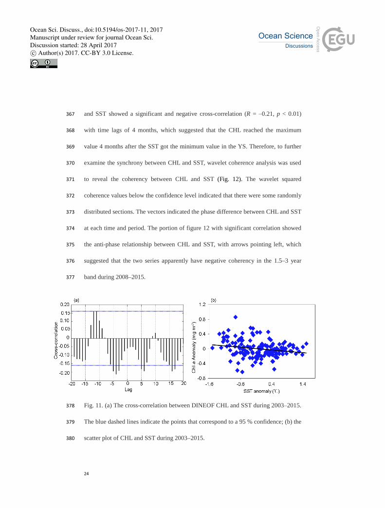
The anti-phase relationships agreed well with the negative correlation 360
coefficients between CHL and SST, which agreed with other researchers (Hou et al., 361
2016). In our study, the statistically significant cross-correlation between the monthly 362
CHL and SST datasets after removing seasonal variations (Fig. 11a) also suggested 363
that variability in CHL was slightly negatively correlated with variability in SST in 364
the YS during the study period. The negative correlation was confirmed also by the 365
scatter plot of CHL and SST (Fig. 11b). The cross-correlation between monthly CHL 366
Ocean Sci. Discuss., doi:10.5194/os-2017-11, 2017Manuscript under review for journal Ocean Sci.Discussion started: 28 April 2017c© Author(s) 2017. CC-BY 3.0 License.
24
and SST showed a significant and negative cross-correlation (R = –0.21, p < 0.01) 367
with time lags of 4 months, which suggested that the CHL reached the maximum 368
value 4 months after the SST got the minimum value in the YS. Therefore, to further 369
examine the synchrony between CHL and SST, wavelet coherence analysis was used 370
to reveal the coherency between CHL and SST (Fig. 12). The wavelet squared 371
coherence values below the confidence level indicated that there were some randomly 372
distributed sections. The vectors indicated the phase difference between CHL and SST 373
at each time and period. The portion of figure 12 with significant correlation showed 374
the anti-phase relationship between CHL and SST, with arrows pointing left, which 375
suggested that the two series apparently have negative coherency in the 1.5–3 year 376
band during 2008–2015. 377
Fig. 11. (a) The cross-correlation between DINEOF CHL and SST during 2003–2015. 378
The blue dashed lines indicate the points that correspond to a 95 % confidence; (b) the 379
scatter plot of CHL and SST during 2003–2015. 380
Ocean Sci. Discuss., doi:10.5194/os-2017-11, 2017Manuscript under review for journal Ocean Sci.Discussion started: 28 April 2017c© Author(s) 2017. CC-BY 3.0 License.

25
Fig. 12. Wavelet coherency between DINEOF CHL and SST during 2003–2015 in the 381
YS. Thin solid lines demarcate the cones of influence and thick solid lines show the 382
95 % confidence levels. The color bar indicates strength of correlation, and the 383
direction of arrow show the correlation type with the right pointing arrows being 384
positive and left pointing arrows being negative. 385
5. Concluding remarks 386
The main purpose of this study was to identify the variability in CHL and SST 387
on both seasonal and inter-annual time scales and its cross relationship based on the 388
long-term, cloud-free, DINEOF CHL and SST datasets. In addition to the EOF, we 389
also applied the wavelet coherency analysis to CHL and SST to determine temporal 390
relations during 2003–2015. 391
Similar with the other middle latitude regions, the CHL variability was 392
dominated generally by a spring bloom with a secondary fall bloom throughout the 393
entire YS region. The EOF1 mode showed stronger seasonal variability in the area 394
Ocean Sci. Discuss., doi:10.5194/os-2017-11, 2017Manuscript under review for journal Ocean Sci.Discussion started: 28 April 2017c© Author(s) 2017. CC-BY 3.0 License.
26
with stronger circulation in the water column. Temporally, the CHL EOF1 mode also 395
exhibited a seasonal cycle with a maximum in late winter and early spring and a 396
minimum in summer and early autumn for each year. This could be explained by the 397
influences of the water currents in the YS. The SST EOF1 mode was dominated by a 398
seasonal cycle: warmest in summer and coldest in winter. Further analysis showed 399
that the magnitude of the seasonal cycle in different regions was a result of water 400
depth and water currents in the YS. There is a strong match between the mean CHL 401
and SST patterns throughout the entire YS region. This relationship can be explained 402
in terms of lower primary production levels that corresponded to stronger 403
stratification of the water column. 404
There were positive trends both for CHL and SST in the inter-annual time scale 405
during 2003–2015. There was a significant negative correlation between CHL and 406
SST with time lags of 4 months. Thus, we speculate that CHL reached the maximum 407
value 4 months later than the SST got the minimum value in the YS. Furthermore, the 408
wavelet power spectrum and the global power spectrum for CHL and SST showed 409
similar periods of variation, and similar synchronized and corresponding patterns of 410
evolution. The dominant periods were 2–4 years during 2003–2015. CHL was 411
significantly associated with SST in the time-frequency domain, and shared the 412
common variation with the period of 1.5–3 years during 2008–2015, based on the 413
wavelet coherence analysis. The CWT and wavelet coherence analysis extend the 414
discussion on the scales of temporal variability and oscillation periods of CHL and 415
SST, and they provided insights into how CHL might vary with SST in the future. 416
Ocean Sci. Discuss., doi:10.5194/os-2017-11, 2017Manuscript under review for journal Ocean Sci.Discussion started: 28 April 2017c© Author(s) 2017. CC-BY 3.0 License.

27
417
Data availability. The SST and CHL datasets used in this study are available 418
at http://oceancolor.gsfc.nasa.gov. 419
420
Competing interests. The authors declare that they have no conflict of interest. 421
422
Acknowledgements. This study was supported by the National Science Foundation of 423
China (41206166); The Science and Technology Development Plan Project of Weihai 424
(2014DXGJ36); The State Key Laboratory of Tropical Oceanography, South China 425
Sea Institute of Oceanology, Chinese Academy of Sciences (LTO1608); The National 426
Natural Science Foundation of China (41676171); Qingdao National Laboratory for 427
Marine Science and Technology of China (2016ASKJ02); The Natural Science 428
Foundation of Shandong Province, China (ZR2010DQ019). 429
References 430
Alvera-Azcárate, A., Vanhellemont, Q., Ruddick, K., Barth, A., and Beckers, J.-M.: 431
2015. Analysis of high frequency geostationary ocean colour data using DINEOF, 432
Estuarine, Cont. Shelf Res., 159, 28–36, 2015. 433
Alvera-Azcárate, A., Barth, A., Parard, G., and Beckers, J.-M.: Analysis of SMOS sea 434
surface salinity data using DINEOF, Remote Sens. Environ, 180, 137–145, 2016. 435
Beckers, J.-M. and Rixen, M.: EOF calculations and data filling from incomplete 436
oceanographic datasets, J. Atmos. Oceanic. Technol., 20, 1839–1856, 2003. 437
Beckers, J.-M., Barth, A. and Alvera-Azcárate, A.: DINEOF reconstruction of 438
Ocean Sci. Discuss., doi:10.5194/os-2017-11, 2017Manuscript under review for journal Ocean Sci.Discussion started: 28 April 2017c© Author(s) 2017. CC-BY 3.0 License.

28
clouded images including error maps-application to the sea surface temperature 439
around Corsican Island, Ocean Sci., 2, 183–199, 2006. 440
Behrenfeld, M. J., O’Malley, R. T. and Siegel, D. A.: 2006. Climate-driven trends in 441
contemporary ocean productivity, Nature, 444, 752–755, 2006. 442
Boyce, D. G., Lewis, M. R. and Worm, B.: Global phytoplankton decline over the past 443
century, Nature, 466, 591–596, 2010. 444
Campbell, J. W.: The lognormal distribution as a model for bio-optical variability in 445
the sea, J. Geophys. Res., 100, 13237–13254, 1995. 446
Chen, C., Beardsley, R., Limeburner, R. and Kim, K.: Comparison of winter and 447
summer hydrographic observations in the Yellow and East China Seas and 448
adjacent Kuroshio during 1986, Cont. Shelf Res., 14, 909–929, 1994. 449
Chu, P., Chen, Y. C., Kuninaka, A.: Seasonal variability of the Yellow Sea/East China 450
sea surface fluxes and thermohaline structure, Adv. Atmos. Sci., 22, 1–20, 2005. 451
Doney, S. C.: Oceanography-Plankton in a warmer world, Nature, 444, 695–696, 452
2006. 453
Gao, S., Wang, H., Liu, G. M. and Li, H.: Spatio-temporal variability of chlorophyll a 454
and its responses to sea surface temperature, winds and height anomaly in the 455
western South China Sea, Acta Oceanol. Sin., 32, 48–58, 2013. 456
Gregg, W. W., Casey, N. W. and McClain, C. R.: Recent trends in global ocean 457
chlorophyll, Geophys. Res. Lett., 32, 259–280, 2005. 458
Grinsted, A., Moore, J. C. and Jevrejeva, S.: Application of the cross wavelet 459
transform and wavelet coherence to geophysical time series, Nonlinear Process. 460
Ocean Sci. Discuss., doi:10.5194/os-2017-11, 2017Manuscript under review for journal Ocean Sci.Discussion started: 28 April 2017c© Author(s) 2017. CC-BY 3.0 License.

29
Geophys, 11, 561–566, 2004. 461
He, R., Weisberg, R. H., 2003. West Florida shelf circulation and temperature budget 462
for 1998 fall transition. Cont. Shelf Res. 23(8), 777–800. 463
He, R., Chen, K., Moore, T. and Li, M.: Mesoscale variations of sea surface 464
temperature and ocean color patterns at the Mid-Atlantic Bight shelfbreak, 465
Geophys. Res. Lett., 37, 493–533, 2010. 466
Hou, X. Y., Dong, Q., Xue, C. J., Wu, S. C.: Seasonal and interannual variability of 467
chlorophyll-a and associated physical synchronous variability in the western 468
tropical Pacific, J. Mar. Syst., 158, 59–71, 2016. 469
Hu, W. and Si, B. C.: Estimating spatially distributed soil water content at small 470
watershed scales based on decomposition of temporal anomaly and time stability 471
analysis. Hydrol. Earth Syst. Sci. 20, 571–587, 2016a. 472
Hu, W. and Si, B. C.: Multiple wavelet coherence for untangling scale-specific and 473
localized multivariate relationships in geosciences, Hydrol. Earth Syst. Sci., 20, 474
3183–3191, 2016b. 475
Huynh, H-N.T., Alvera-Azcárate, A., Barth, A. and Beckers, J.-M.: Reconstruction 476
and analysis of long-term satellite-derived sea surface temperature for the South 477
China Sea, J. Oceanogr., 72, 707–726, 2016. 478
Ichikawa, H. and Beardsley, R. C.: The current system in the Yellow and East China 479
Seas, J. Oceanogr., 58, 77–92, 2002. 480
Li, Y. Z. and He, R. Y.: Spatial and temporal variability of SST and ocean color in the 481
Gulf of Maine based on cloud-free SST and chlorophyll reconstructions in 482
Ocean Sci. Discuss., doi:10.5194/os-2017-11, 2017Manuscript under review for journal Ocean Sci.Discussion started: 28 April 2017c© Author(s) 2017. CC-BY 3.0 License.
30
2003-2012, Remote Sens. Environ., 144, 98–108, 2014. 483
Lie, H.-J., Cho, H.-C. and Lee, S.: Tongue-shaped frontal structure and warm water 484
intrusion in the southern Yellow Sea in winter, J. Geophys. Res., 114, 362–370, 485
2009. 486
Lin, C., Ning, X., Su, J., Lin, Y. and Xu, B.: Environmental changes and the responses 487
of the ecosystems of the Yellow Sea during 1976–2000, J. Mar. Syst., 55, 223–488
234, 2005. 489
Liu, D. Y. and Wang, Y. Q.: Trends of satellite derived chlorophyll-a (1997–2011) in 490
the Bohai and Yellow Seas, China: Effects of bathymetry on seasonal and 491
inter-annual patterns, Prog. Oceanogr., 116, 154–166, 2013. 492
Liu, M., Liu, X., Ma, A., Li, T. and Du, Z.: Spatio-temporal stability and abnormality 493
of chlorophyll-a in the Northern South China Sea during 2002–2012 from 494
MODIS images using wavelet analysis, Cont. Shelf Res., 75, 15–27, 2014. 495
Messié, M. and Chavez, F.: Global modes of sea surface temperature variability in 496
relation to regional climate indices, J. Clim., 24, 4314–4331, 2011. 497
Messié, M., Radenac, M.: Seasonal variability of the surface chlorophyll in 498
thewestern tropical Pacific fromSeaWiFS data. Deep-Sea Res. I Oceanogr. Res. 499
Pap. 53 (10), 1581–1600, 2006. 500
Miles, T. N. and He, R.: Temporal and spatial variability of CHL and SST on the 501
South Atlantic Bight: Revisiting with cloud-free reconstructions of MODIS 502
satellite imagery, Cont. Shelf Res., 30, 1951–1962, 2010. 503
Moradi, M., Kabiri, K.: Spatio-temporal variability of SST and Chlorophyll-a from 504
Ocean Sci. Discuss., doi:10.5194/os-2017-11, 2017Manuscript under review for journal Ocean Sci.Discussion started: 28 April 2017c© Author(s) 2017. CC-BY 3.0 License.

31
MODIS data in the Persian Gulf, Mar. Pollut. Bull., 98, 14–25, 2015. 505
Muller-Karger, F. E., Hu, C., Andréfouët, S., Varela, R. and Thunell, R.: The color of 506
the coastal ocean and applications in the solution of research and management 507
problems. Remote Sensing of Coastal Aquatic Environments. Springer, 101–127, 508
2005. 509
Ng, E. K. W. and Chan, J. C. L.: Geophysical applications of partial wavelet 510
coherence and multiple wavelet coherence, J. Atmos. Ocean. Technol., 29, 1845–511
1853, 2012. 512
North, G. R., Bell, T. L., Cahalan, R. F. and Moeng, F. J.: Sampling errors in the 513
estimation of empirical orthogonal functions, Mon. Wea. Rev. 110, 699–706, 514
1982. 515
O’Reilly, J. E., Evans-Zetlin, C. and Busch. D. A.: Primary production. In R. H. 516
Backus (Ed), Georges Bank ( 221–233). Cambridge, MA: MTT Press, 1987. 517
Olita, A., Ribotti, A., Sorgente, R., Fazioli, L. and Perilli, A.: SLA-chlorophyll-a 518
variability and covariability in the Algero-Provençal Basin (1997–2007) through 519
combined use of EOF and wavelet analysis of satellite data, Ocean Dyn., 61, 89–520
102, 2011. 521
Park, K. A., Chung, J. Y., Kim, K. and Cornillon, P. C.: Wind and bathymetric 522
forcing of the annual sea surface temperature signal in the East (Japan) Sea, 523
Geophys. Res. Lett., 32, 215–236, 2005. 524
Park, K. A., Lee, E. Y., Chang, E. and Hong, S. W.: Spatial and temporal variability of 525
sea surface temperature and warming trend in the Yellow Sea, J. Mar. Syst., 143, 526
Ocean Sci. Discuss., doi:10.5194/os-2017-11, 2017Manuscript under review for journal Ocean Sci.Discussion started: 28 April 2017c© Author(s) 2017. CC-BY 3.0 License.
32
24–38, 2015. 527
She, D. L., Fei, Y. H., Chen, Q. and Timm, L. C.: Spatial scaling of soil salinity 528
indices along a temporal coastal reclamation area transect in China using wavelet 529
analysis, Arch. Agron. Soil Sci., 62, 1625–1639, 2016. 530
Shi, W. and Wang, M.: Satellite views of the Bohai Sea, Yellow Sea, and East China 531
Sea, Prog. Oceanogr., 104, 30–45, 2012. 532
Sirjacobs, D., Alvera-Azcárate, A., Barth, A., Lacroix, G., Park, Y., Nechad, B. and 533
Beckers, J.-M.: Cloud filling of ocean colour and sea surface temperature remote 534
sensing products over the Southern North Sea by the Data Interpolating Empirical 535
Orthogonal Functions methodology, J. Sea Res., 65, 114–130, 2011. 536
Smith, V. H.: Responses of estuarine and coastal marine phytoplankton to nitrogen 537
and phosphorus enrichment, Limnol. Oceanogr., 51, 377–384, 2006. 538
Teague, W. J. and Jacobs, G. A.: Current observations on the development of the 539
Yellow Sea Warm Current, J. Geophys. Res., 105, 3401–3411, 2000. 540
Thomas, A.C., Ted Strub, P., Weatherbee, R.A., James, C.; Satellite views of Pacific 541
chlorophyll variability: comparisons to physical variability, local versus nonlocal 542
influences and links to climate indices. Deep-Sea Res. II Top. Stud. Oceanogr. 543
77–80 (0), 99–116,2012. 544
Townsend, D. W., Rebuck, N. D., Thomas, M. A., Karp-Boss, L. and Gettings, R. M.: 545
A changing nutrient regime in the Gulf of Maine, Cont. Shelf Res., 30, 820–832, 546
2010. 547
Tseng, C., Lin, C., Chen, S. and Shyu, C.: Temporal and spatial variations of sea 548
Ocean Sci. Discuss., doi:10.5194/os-2017-11, 2017Manuscript under review for journal Ocean Sci.Discussion started: 28 April 2017c© Author(s) 2017. CC-BY 3.0 License.
33
surface temperature in the East China Sea, Cont. Shelf Res., 20, 373–387, 2000. 549
Venables, W. N. and Ripley, B. D.: Modern Applied statistics with S, fourth ed. 550
Springer-Verlag, New York, 2002. 551
Volpe, G., Nardelli, B. B., Cipollini, P., Santoleri, R. and Robinson, I. S.: Seasonal to 552
interannual phytoplankton response to physical processes in the Mediterranean 553
Sea from satellite observations, Remote Sens. Environ., 117, 223–235, 2012. 554
Wei, H., Shi, J., Lu, Y. and Peng, Y.: Interannual and long-term hydrographic changes 555
in the Yellow Sea during 1977–1998, Deep-Sea Res. II., 57, 1025–1034, 2010. 556
Wei, Q. S., Li, X. S., Wang, B. D., Fu, M. Z., Ge, R. F. and Yu, Z. G.: Seasonally 557
chemical hydrology and ecological responses in frontal zone of the central 558
southern Yellow Sea, J. Sea Res., 112, 1–12, 2016. 559
Werdell, P. J., Bailey, S. W., Franz, B. A., Harding Jr., L. W., Feldman, G. C. and 560
McClain, C. R.: Regional and seasonal variability of chlorophyll-a in Chesapeake 561
Bay as observed by SeaWiFS and MODIS-aqua, Remote Sens. Environ., 113, 562
1319–1330, 2009. 563
Wilson, C. and Coles, V. J.: Global climatological relationships between satellite 564
biological and physical observations and upper ocean properties, J. Geophys. Res., 565
110, 1–14, 2005. 566
Xie, S. P., Hafner, J., Tanimoto, Y., Liu, W. T., Tokinaga, H. and Xu, H.: 567
Bathymetric effect on the winter sea surface temperature and climate of the 568
Yellow and East China Seas, Geophys. Res. Lett., 29, 2228–2231, 2002. 569
Xu, M., Liu, Q. H., Zhang, Z. N. and Liu, X. S.: Response of free-living marine 570
Ocean Sci. Discuss., doi:10.5194/os-2017-11, 2017Manuscript under review for journal Ocean Sci.Discussion started: 28 April 2017c© Author(s) 2017. CC-BY 3.0 License.

34
nematodes to the southern Yellow Sea Cold Water Mass, Mar. Pollut. Bull., 105, 571
58–64, 2016. 572
Yamaguchi, H., Kim, H. C., Son, Y. B., Kim, S. W., Okamura, K., Kiyomoto, Y. and 573
Ishizaka, J.: Seasonal and summer-interannual variations of SeaWiFS chlorophyll 574
a in the Yellow Sea and East China Sea, Prog. Oceanogr., 105, 22–29, 2012. 575
Yan, X. H., Shubel, J. R. and Pritchard, D. W.: Oceanic upper mixed depth 576
determination by the use of satellite data, Remote Sens. Environ., 32, 55–74, 577
1990. 578
Yeh, S. W. and Kim, C. H.: Recent warming in the Yellow/East China Sea during 579
winter and the associated atmospheric circulation, Cont. Shelf Res., 30, 1428–580
1434, 2010. 581
Yu, F., Zhang, Z. X., Diao, X. Y. and Guo, J. S.: Observational evidence of the Yellow 582
Sea Warm Current, Chin. J. Oceanol. Limnol., 28, 677–683, 2010. 583
Zhang, S. W., Wang, Q. Y., Lü, Y., Cui, H. and Yuan, Y. L.: Observation of the 584
seasonal evolution of the Yellow Sea Cold Water Mass in 1996–1998, Cont. Shelf 585
Res., 28, 442–457, 2008. 586
Ocean Sci. Discuss., doi:10.5194/os-2017-11, 2017Manuscript under review for journal Ocean Sci.Discussion started: 28 April 2017c© Author(s) 2017. CC-BY 3.0 License.