Interactive Sound Propagation using Compact Acoustic ...gamma.cs.unc.edu/CATR/part.pdf · transfer, higher-order reﬂections, interactive applications 1. INTRODUCTION Realistic sound

Interactive Sound Propagation using Compact AcousticTransfer OperatorsLAKULISH ANTANI and ANISH CHANDAKUniversity of North Carolina at Chapel HillandLAURI SAVIOJAAalto UniversityandDINESH MANOCHAUniversity of North Carolina at Chapel Hill

We present an interactive sound propagation algorithm that can computehigh orders of specular and diffuse reflections as well as edge diffractionsin response to moving sound sources and a moving listener. Our formulationis based on a precomputed acoustic transfer operator, which we compactlyrepresent using the Karhunen-Loeve transform. At runtime, we use a two-pass approach that combines acoustic radiance transfer with interactive raytracing to compute early reflections as well as higher-order reflections andlate reverberation. The overall approach allows accuracy to be traded offfor improved performance at run-time, and has a low memory overhead.We demonstrate the performance of our algorithm on different scenarios,including an integration of our algorithm with Valve’s Source game engine.

Categories and Subject Descriptors: I.3.7 [Computer Graphics]: Three-Dimensional Graphics and Realism—Radiosity; I.3.8 [Computer Graph-ics]: Applications—Sound rendering; H.5.5 [Information Systems]: Infor-mation Interfaces and Presentation—Sound and music computing

General Terms: Real-time Rendering, Geometric Acoustics

Additional Key Words and Phrases: sound propagation, acoustic radiancetransfer, higher-order reflections, interactive applications

1. INTRODUCTION

Realistic sound propagation and rendering can add a whole newlayer of realism to interactive applications such as video games andvirtual environments. Sound propagation in a scene refers to themodeling of the sound heard by the listener after the sound emit-

Permission to make digital or hard copies of part or all of this work forpersonal or classroom use is granted without fee provided that copies arenot made or distributed for profit or commercial advantage and that copiesshow this notice on the first page or initial screen of a display along withthe full citation. Copyrights for components of this work owned by othersthan ACM must be honored. Abstracting with credit is permitted. To copyotherwise, to republish, to post on servers, to redistribute to lists, or to useany component of this work in other works requires prior specific permis-sion and/or a fee. Permissions may be requested from Publications Dept.,ACM, Inc., 2 Penn Plaza, Suite 701, New York, NY 10121-0701 USA, fax+1 (212) 869-0481, or [email protected]© YYYY ACM 0730-0301/YYYY/12-ARTXXX $10.00

DOI 10.1145/XXXXXXX.YYYYYYYhttp://doi.acm.org/10.1145/XXXXXXX.YYYYYYY

ted from each source undergoes reflections, diffraction and absorp-tion through the scene, taking into account source and listener po-sitions within the scene along with surface material properties. At abroad level, sound propagation effects in an acoustic environmentare composed of two parts: early reflections (ER) and late reverber-ation (LR) ([Kuttruff 1991], pp. 97). For the listener, ER helps inlocalization and conveys spatial information about an environment,while LR enhances immersion, giving an impression of the sizeof the environment, level of furnishing and absorptivity ([Kuttruff1991], pp. 98, 194). In order to generate plausible sound rendering,it is important to model both of these parts.

Accurate offline algorithms for sound propagation are limitedto static sources and/or listeners. Several algorithms have beenproposed for interactive sound propagation in dynamic scenes, butthey are limited to modeling early reflections only. As a result,there has been recent interest in developing precomputation-basedalgorithms to model higher-order reflections. However, thesemethods have a very high memory overhead, or require the sceneto be composed of cells and portals (see Section 2.1 for moredetails).

Main Results We present a novel geometric sound propagation al-gorithm that computes diffuse and specular reflections as well asedge diffractions at near-interactive rates. In order to model higher-order reflections and diffraction, our algorithm precomputes anacoustic transfer operator that models how sound energy prop-agates between surfaces. We use a scene-dependent Karhunen-Loeve transform (KLT) for compactly representing the transfer op-erators. At runtime, we use a two-pass method that uses the transferoperator to compute higher-order reflections and diffraction, alongwith interactive ray tracing to model early reflections and diffrac-tion.

Some of the main benefits of our approach include:

—Compact representation: Our compression technique, based onKLT, results in low memory overhead for the acoustic transferoperators, resulting in a compression factor of up to two ordersof magnitude over time-domain or frequency-domain represen-tations.

—Runtime control between accuracy and performance: Ourchoice of basis for representing the acoustic transfer operatorhas the additional advantage of allowing control over approxi-mation errors, and thereby trading off accuracy for performancein interactive applications.

ACM Transactions on Graphics, Vol. VV, No. N, Article XXX, Publication date: Month YYYY.

2 • L. Antani et al.

—Moving sources and listeners: Our precomputed acoustic trans-fer operator is defined in terms of samples distributed over thesurfaces of a static scene. As a result, we can efficiently handlemoving sources and listeners.

—Occlusion of sound by dynamic objects: Our algorithm canhandle (to a limited extent) the effect of introducing a dynamicobject on the sound field at the listener – due to occlusion ofsound emitted from the source by moving obstacles and the sub-sequent effect of the occlusion on propagated sound, or due toocclusion of propagated sound by moving obstacles before itreaches the listener.

In practice, our algorithm can handle indoor models at nearlyinteractive rates, i.e. 5−10 frames per second on a modern desktopcomputer. The memory overhead of storing the precomputedtransfer operators is typically a few dozen megabytes. We havealso integrated our algorithm with Valve’s Source engine, and useit to provide plausible sound propagation effects during real-timegameplay.

Outline The rest of the paper is organized as follows. Section 2provides a brief overview of prior art. Section 3 presents our for-mulation and compression method for acoustic transfer operators.Section 4 describes our run-time algorithm. We describe our imple-mentation in Section 5 and highlight the performance on differentbenchmarks, including the Source engine. Finally, we analyze theapproach in Section 6 and compare it with prior approaches.

2. BACKGROUND

In this section, we give a brief overview of related work and intro-duce some background material used in the rest of the paper.

2.1 Related Work

We now present some key approaches used for sound propagation.

Wave-based Acoustics The propagation of sound in a medium isdescribed by the acoustic wave equation, a second-order partialdifferential equation. Several numerical methods are known forsolving the wave equation, such as finite-element [Ihlenburg1998] and boundary-element methods [Ciskowski and Brebbia1991], finite-difference time-domain methods [Savioja et al. 1994;Botteldooren 1995], etc. These techniques are the most accurate interms of modeling sound propagation in a scene. In spite of recentadvances [Raghuvanshi et al. 2009], these methods are limitedto static scenes and can be very slow for high-frequency soundsources.

Geometric Acoustics Most sound propagation techniques usedin interactive applications are based on geometric methods. Thesetechniques tend to be accurate for high-frequency sources. Someof the commonly used methods are based on ray tracing [Saviojaet al. 1999; Kapralos et al. 2004; Bertram et al. 2005; Lentz et al.2007], which can be used to model both diffuse and specularreflections. Recent video games such as Crackdown use ray tracingto compute low-order sound propagation effects. In order toovercome the sampling issues inherent in ray tracing, techniquesbased on volume tracing [Funkhouser et al. 1998; Taylor et al.2009] and image sources [Allen and Berkley 1979; Laine et al.2009; Chandak et al. 2009] have been developed. For static scenes,radiosity [Tsingos and Gascuel 1997; Nosal et al. 2004; Alarcaoet al. 2009] or radiance transfer [Siltanen et al. 2007; Siltanen et al.2009] methods can be used to model reflections from surfaces with

arbitrary BRDFs. Many techniques have also been designed tomodel edge diffraction [Svensson et al. 1999; Tsingos et al. 2001;Stephenson 2010].

Statistical Acoustics Most current video games use acousticparameters such as reverberation time to model the acoustics ofa scene. These can be derived from statistical models ([Kuttruff1991], pp. 119) and/or controlled by an artist. There has beenrecent work on statistical estimation of diffuse reverberationproperties [Taylor et al. 2009]. In practice, statistical models aretypically valid only for simple single or coupled rooms [Summerset al. 2004], and are not considered as accurate as other methods[Stavrakis et al. 2008].

Precomputed Sound Propagation The problem of precomputingsound propagation effects for interactive applications has receivedsignificant attention in recent years. Cell-and-portal-based scenesubdivision has been exploited to model the propagation of soundbetween cells via portals [Foale and Vamplew 2007; Stavrakiset al. 2008]. Other methods include precomputing image sourcegradients to quickly estimate specular reflections at run-time[Tsingos 2009], precomputing acoustic radiance transfer fromstatic sources [Siltanen et al. 2009], using a numerical waveequation solver to precompute the acoustic response of a scenefrom several sampled source positions [Raghuvanshi et al. 2010],and precomputing linear operators to model diffuse reflections ofsound in the frequency domain [Antani et al. 2011].

Interactive Acoustics For interactive applications, efficientscalable algorithms based on hierarchical sound source clusteringhave been developed [Moeck et al. 2007] in order to rendersound from large numbers of sources. Many scalable soundsynthesis algorithms have also been developed, which can renderhigh-quality, physically-based sound due to collisions [Jameset al. 2006; Raghuvanshi and Lin 2006; Bonneel et al. 2008;Chadwick et al. 2009]. These algorithms manage the complexityof sound simulation by controlling the detail in the generation ofsound (either by culling sources, or by simplifying the physicalmodel used to generate the sound). In contrast, our algorithmcontrols the detail in the propagation of sound, by simplifying therepresentation of an acoustic transfer operator.

Precomputed Light Transport Radiosity [Goral et al. 1984] is theclassic precomputed light transport algorithm. However, it com-putes a global illumination solution that needs to be recomputedwhenever the light source moves. In contrast, precomputed ra-diance transfer (PRT) algorithms decouple light transport effectsfrom the light source positions by computing a linear operator thatdefines how a variable light source configuration affects the radi-ance at surface sample points. PRT techniques can support bothdistant [Sloan et al. 2002] and local [Kristensen et al. 2005; Lehti-nen et al. 2008] source configurations. We use many of these ideasto formulate our acoustic transfer operators.

2.2 Impulse Responses and Echograms

Sound travels much slower (340 m/s in air) than light (3×108 m/s).Hence, while light transport algorithms can compute steady-statevalues of lighting in the scene and neglect transient effects, it is vi-tal to capture the time variation of the sound energy distribution in ascene. It is this time variation which gives rise to echoes and rever-beration in large rooms. The additional dimension of time makes it


Interactive Sound Propagation using Compact Acoustic Transfer Operators • 3

difficult to apply light transport algorithms directly to model soundpropagation.

Physically, the sound emitted by a source is a pressure wave,denoted by ps(t). The sound waves travel through the scene, un-dergoing reflection, diffraction and absorption. The listener thenreceives a propagated pressure wave, pl(t). Since room acous-tics can be modeled as a linear time-invariant system ([Kuttruff1991], pp. 19), the sound heard at the listener can be obtained aspl(t) = hs,l(t)⊗ ps(t), where hs,l(t) is the impulse response (IR)between the source and listener and ⊗ is the time-domain convolu-tion operator. Intuitively, an IR is the signal received at the listenerif the source emits a unit impulse δ(t). An echogram is defined asthe energy contained in an IR as a function of time, and is propor-tional to the square of the IR. In the rest of this work, we focus oncomputing echograms.

2.3 Acoustic Rendering Equation

Analogous to the definition of radiance in visual rendering, acous-tic radiance at a point x, denoted by L(x,Ω, t), is defined as theoutgoing sound energy flux at point x per unit area per unit solidangle along direction Ω, as a function of time t. Similarly, we candefine acoustic irradiance at a point x, denoted by E(x, t), as theincident sound energy flux at point x per unit area as a function oftime. For a point listener, the acoustic irradiance is proportional tothe echogram, and hence to the square of the IR.

The propagation of sound in a scene can be modeled using an ex-tension of the standard graphics rendering equation [Kajiya 1986],called the acoustic rendering equation [Siltanen et al. 2007]:

L(x,Ω, t) = L0(x,Ω, t) (1)

+

∫S

R(x, x′,Ω, t)L

(x′,

x− x′

|x− x′|, t

)dx′

where L is the total outgoing acoustic radiance, L0 is the emittedacoustic radiance and R is the reflection kernel, which describeshow radiance at point x′ influences radiance at point x (Ω is thefinal radiance direction at x; the incident radiance direction at x isimplicit in the specification of x′):

R(x, x′,Ω, t) = ρ(x, x′,Ω, t)G(x, x′)V (x, x′)P (x, x′, t). (2)

Here, ρ is the BRDF of the surface at x, G is the form factor be-tween x and x′, V is the point-to-point visibility function, and Pis a propagation term [Siltanen et al. 2007] that accounts for prop-agation delays. We use this equation to define the acoustic transferoperators.

The above equations represent the acoustic rendering equationin the time domain. Hence, the BRDF (and other terms) need tobe convolved with the acoustic radiance; the convolution operatorshave been hidden in the equations for brevity. Alternatively, onecould formulate the acoustic rendering equation in the frequencydomain (replacing the time variable t with the angular frequencyω); in the frequency domain the BRDF (and other terms) indeedare multiplied with the acoustic radiance. Thus one can model ar-bitrary frequency-dependent material properties using the acousticrendering equation.

3. ACOUSTIC TRANSFER OPERATOR

The goal of our algorithm is to efficiently compute the late re-sponse (LR), i.e., higher-order (i.e., beyond 2-3 orders) reflectionsand edge diffraction of sound, which changes in response to a mov-ing source and a moving listener in a scene. We accomplish this by

precomputing an acoustic transfer operator which models the prop-agation of acoustic radiance between samples distributed over thesurface of the scene. In this sense, our algorithm is analogous toPRT algorithms for light transport problems. The acoustic trans-fer operator is defined by writing the incident form of the acousticrendering equation in terms of a linear operator:

L(x,Ω, t) = L0(x,Ω, t) +RL(x,Ω, t)

= T L0(x,Ω, t), (3)

where L0(x,Ω, t) represents the direct acoustic radiance incidentat surface point x, L(x,Ω, t) represents the indirect acoustic radi-ance incident at x after multiple reflections and diffraction throughthe scene, R is a linear operator corresponding to the reflectionkernel in Equation 2 and T = (I − R)−1 is the acoustic transferoperator.

We assume that acoustic radiance at a surface sample does notvary with direction (i.e., the surface samples are diffuse emittersand receivers). In other words, the transfer operator models soundenergy which is emitted uniformly in all directions from a givensurface sample, and propagates through the scene (undergoing sev-eral diffuse and specular reflections as well as diffraction) until thepropagation is finally terminated upon incidence at some other sur-face sample. The propagated, incident sound field is averaged overall incidence directions, resulting in a directionally-invariant in-direct acoustic radiance at each surface sample. This simplifyingassumption is motivated by the fact that after a few orders of re-flection, most of the sound energy in a scene would have typicallyundergone diffuse reflections [Kuttruff 1995]. This may result insome higher-order echoes being replaced with reverberation, butcan be corrected when computing the early response. We now de-scribe our approach for computing a compact representation of theacoustic transfer operator.

3.1 Transfer Operator Precomputation

In order to define the acoustic transfer operator for the scene,we first sample n points on the surface of the scene using area-weighted sampling [Hasan et al. 2006] (Figure 1 (b)). We thenconstruct a compact, scene-dependent KLT basis for represent-ing echograms (Figure 1 (c)), which we then use to compressechograms computed between each surface sample (Figure 1 (d)).

We use energy-based path tracing (i.e., Monte Carlo integrationof the acoustic rendering equation) to compute the sample-to-sample echograms. When each path encounters a geometricprimitive, it can be diffusely reflected, specularly reflected ordiffracted, depending on material properties. Attenuations areapplied according to standard geometric acoustics models asdiscussed below.

Diffuse Reflections Rays are diffusely reflected as per the Lam-bertian model by randomly sampling a direction on the hemisphereat the point of incidence, and sending a reflected ray along thesampled direction. The ray’s energy is attenuated by the frequency-dependent diffuse coefficient d(ν) = (1− α(ν))σ(ν), where α(ν)is the frequency-dependent absorption coefficient and σ(ν) is thefrequency-dependent scattering coefficient of the surface material.

Specular Reflections Specular reflection of rays is performedby reflecting incident rays as per the laws of reflection. Theray’s energy is attenuated by the frequency-dependent specularcoefficient s(ν) = (1− α(ν))(1− σ(ν)).



Fig. 1: Overview of our algorithm. Top row: Precomputation. Bottom row: Run-time interactive sound propagation.

Edge Diffraction Diffraction is modeled using an energy-basedray tracing model derived from Heisenberg’s uncertainty principle[Stephenson and Svensson 2007; Stephenson 2010]. Rays whichpass sufficiently close to a diffracting edge [Stephenson and Svens-son 2007] are diffracted by deviating them in the plane normal tothe diffracting edge. The angle of deviation is randomly sampledfrom a frequency-dependent probability distribution.

3.2 Echogram Representation

In order to capture closely-spaced echoes, which may arise in 2nd

or 3rd order reflections captured in the transfer operator, we sampleechograms at the audio sampling rate of 48 kHz. As a result, it isimpractical to store precomputed sample-to-sample echograms inthe time domain, since this would require 192 kB per second perechogram. For n ≈ 256 surface samples, this would result in thetransfer operator requiring 12 GB of storage per second.

Frequency-domain representations have been used in priorprecomputation-based sound propagation algorithms, but require avery large number of coefficients (m ≈ 1024) to represent eitherthe echograms themselves [Siltanen et al. 2009], or the decay en-velopes of the echograms [Stavrakis et al. 2008] (which cannot beused to model sharp echoes arising from 2nd or 3rd order reflec-tions).

Commonly used signal compression techniques are based onrepresenting the signals using transforms such as the Fourier trans-form, the discrete cosine transform (DCT) and the related modifieddiscrete cosine transform (MDCT) [Wang 2003], and wavelet rep-resentations. Fourier and DCT representations require a few thou-sand coefficients [Stavrakis et al. 2008; Siltanen et al. 2009] in or-der to represent the wide range of audible sound frequencies. Whilethe MDCT and wavelet transforms are typically sparse, they too re-quire hundreds of coefficients in order to represent middle-to-high-frequency reverberation in large spaces. Ideally, we would prefer abasis in which echograms can be represented using relatively fewcoefficients.

For this, we use a scene-dependent Karhunen-Loeve basis, de-rived using the Karhunen-Loeve Transform (KLT) [Loeve 1978].The KLT is defined as follows. In order to derive an orthogonalbasis for a d-dimensional vector space S, we first randomly sam-ple some number (say p) of vectors in the space. These vectors arewritten as column vectors and placed side-by-side to form the data

matrix Ad×p (subscripts denote matrix dimensions). We can thenuse the singular value decomposition (SVD) to decompose the datamatrix: Ad×p = Ud×pΣp×pV

tp×p. The columns of the orthogonal

matrix U are then used as a basis set for S.To generate an orthogonal basis for sample-to-sample echograms

in a given scene, we first randomly choose p pairs of surface sam-ples, and compute echograms between them (using path tracing).The dimension of the vector space in which all echograms lie isequal to the number of samples used to represent the echograms inthe time domain. These echograms are used to form the data ma-trix, and then the SVD is used to compute the KLT basis matrix U.Since the basis vectors are sorted in decreasing order of singularvalues, we can truncate U and retain only the first m columns. Asdemonstrated in the accompanying video, the approximation errorcan be barely perceptible (in our benchmarks), even with very fewbasis vectors (m ≈ 32− 64).

In essence, this formulation “learns” a good basis for repre-senting echograms in a given scene by using several exampleechograms computed in the scene. Assuming the surface sam-ple pairs used to generate the example echograms are distributedthroughout the scene, the Karhunen-Loeve transform can be usedto estimate a basis of echograms that requires the fewest numberof coefficients to represent an echogram in the scene for a givenapproximation error. Furthermore, since the storage and time com-plexity of this algorithm scales linearly with m, we choose theKarhunen-Loeve basis to represent the acoustic transfer operatorscompactly.

4. RUN-TIME SOUND PROPAGATION

At run-time, we use an approach similar to prior visual renderingalgorithms [Wallace et al. 1987] and compute sound propagationeffects using a two-pass algorithm (see Figure 1). The two passeswork as follows:

(1) Early Response using Ray Tracing. Since low-order specularreflections and diffraction are important for sound localization,low-order reflections (diffuse and specular) and edge diffrac-tions are computed using path tracing [Bertram et al. 2005].

(2) Late Response using Radiance Transfer. We analyticallycompute the direct echogram at each surface sample due tothe (potentially moving) source(s) (Figure 1 (f)). The acoustic



transfer operator is then applied to the direct echograms; thisyields echograms at each surface sample which model higher-order reflections and diffraction. The resulting echograms aregathered from the surface samples at the listener (Figure 1 (g))to quickly compute the higher-order echogram from a movingsource to a moving listener (Figure 1 (h)).

We now detail each pass of our algorithm.

4.1 Acoustic Radiance Transfer

The direct echogram due to a single source at surface sample j canbe completely characterized by a delayed impulse with (distance)attenuation asj and a delay dsj . Similarly, the response at a listenerdue to direct sound along each gather ray i can be completely char-acterized by a delayed impulse with (distance) attenuation ali and adelay dli.

For simplicity, the BRDFs at the first and last reflections are mul-tiplied into the acoustic transfer operator. Furthermore, for simplic-ity of exposition, we assume that the number of gather rays tracedfrom the listener is also n; in practice, we trace O(n) gather rays,with the constant factor chosen based on run-time performance. Aseach gather ray hits a point on the surface of the scene, the pointis mapped to a surface sample using nearest-neighbor interpola-tion. We denote the surface sample corresponding to gather ray iby S(i).

These attenuations and delays are then combined with the com-pressed acoustic transfer operator to compute the final echogram asfollows. We denote the precomputed echogram from sample j tosample S(i) by Li,j(t). Then the energy received at the listener viapropagation paths whose first reflection occurs at sample j and lastreflection occurs at sample S(i) is given by:

Ei,j(t) = asjaliLi,j(t− dsj − dli), (4)

and the final echogram at the listener is obtained by adding togetherenergy received from all possible propagation paths:

E(t) =

n∑i=1

n∑j=1

asjaliLi,j(t− dsj − dli). (5)

Since the sample-to-sample echograms in the transfer operator arestored in a basis with m coefficients, we use the basis expansion toobtain:

Li,j(t) =

m∑k=1

αki,jb

k(t) (6)

E(t) =

m∑k=1

( n∑i=1

n∑j=1

asjaliα

ki,j

)bk(t− dsj − dli) (7)

where bk denotes the kth basis function and the α’s are coefficientsof echograms in the basis space. The above expression can be re-formulated as a sum of convolutions:

E(t) =

m∑k=1

Hk(t)⊗ bk(t) (8)

Hk(t) =

n∑i=1

n∑j=1

asjaliα

ki,jδ(t− dsj − dli) (9)

Therefore, at run-time, we use the source position to quicklyupdate asj and dsj ; and the listener position to quickly update

ali and dli. These are used along with the compressed transferoperator to construct the convolution filters Hk(t); convolving theechogram basis functions with these filters and accumulating theresults yields an echogram representing higher-order reflectionsand diffraction from the source to the listener.

4.2 Low-Order Effects

Since we assume that surface samples are diffuse emitters and re-ceivers, the radiance transfer pass cannot model all kinds of prop-agation paths. Consider a variant of Shirley’s regular expressionnotation for propagation paths, with D denoting a diffuse reflec-tion, S denoting a specular reflection, and E denoting an edgediffraction. Then the radiance transfer pass is restricted to comput-ing D(D|S|E)∗D paths.

However, low-order specular reflections and diffraction provideimportant directional cues to the listener ([Kuttruff 1991], pp. 194).Therefore, in the first pass of our algorithm, low-order path trac-ing is performed to compute 1-3 orders of specular reflections andedge diffraction as well as first-order diffuse reflections. At eachspecular reflection or edge diffraction, energy can be converted todiffuse energy and transferred to the precomputed transfer opera-tor, allowing paths of the form (S|E)q(D|S|E)∗(S|E)q (for lowvalues of q) to be modeled, thus allowing low-order purely spec-ular and purely diffraction paths to be modeled. As can be seenfrom the corresponding regular expressions, the paths modeled inthe first and second passes are disjoint (i.e., no path is traced in bothpasses), hence the echograms from each pass can be directly added,along with the direct source-to-listener contribution, to determinethe final echogram at the listener.

4.3 Dynamic Scenes

The acoustic transfer operator is inherently decoupled from bothsource and listener positions. As a consequence of this formula-tion, our algorithm can compute higher-order sound propagationin scenes with moving sources and listeners, as mentioned above.Moreover, the computation of early reflections is performed usingray tracing, and hence we can handle fully dynamic scenes in theER pass.

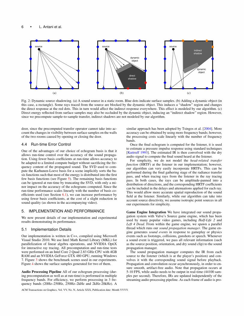
Dynamic objects may also affect the late response. We use inter-active ray tracing [Taylor et al. 2009] to compute direct echogramsat each surface sample (Figure 2 (a)). As a result, these rays canintersect and be blocked by dynamic objects (Figure 2 (b)). This al-lows dynamic objects to induce a “shadow” region and reduce theenergy in the direct echograms at the surface samples in the shadowregion (see Figure 2 (b)). Since these (modified) direct echogramsare used as input to the precomputed acoustic transfer operator inthe first pass, our formulation allows dynamic objects to affect (toa limited extent) the propagated sound field heard at the listener inthe LR pass. Similarly, since interactive ray tracing is used in thefinal gather step, reflected and/or diffracted sound can be occludedby a dynamic object before it reaches the listener.

However, since the transfer operator is pre-computed for surfacesamples defined over static geometry only, we cannot model reflec-tions or inter-reflections off dynamic objects in the radiance trans-fer pass. For example, we can only model ER (and not LR) due tosound reflecting off a moving car. Furthermore, since the transferoperator is computed over static surfaces only, we cannot model“indirect shadow” regions – i.e., occlusion of reflected days by dy-namic objects (Figure 2 (c)). For example, we cannot accuratelymodel the case where two static rooms are separated by a dynamic



source

(a)

source

dynamicobject

directshadow

(b)

source

directshadow

indirectshadow

dynamicobject

(c)

Fig. 2: Dynamic source shadowing. (a) A sound source in a static room. Blue dots indicate surface samples. (b) Adding a dynamic object (inthis case, a rectangle). Some rays traced from the source are blocked by the dynamic object. This induces a “shadow” region and changesthe direct response at the red dots. This in turn would affect the indirect response everywhere. This effect is modeled by our algorithm. (c)Direct energy reflected from surface samples may also be occluded by the dynamic object, inducing an “indirect shadow” region. However,since we precompute sample-to-sample transfer, indirect shadows are not modeled by our algorithm.

door, since the precomputed transfer operator cannot take into ac-count the changes in visibility between surface samples on the wallsof the two rooms caused by opening or closing the door.

4.4 Run-time Error Control

One of the advantages of our choice of echogram basis is that itallows run-time control over the accuracy of the sound propaga-tion. Using fewer basis coefficients at run-time allows accuracy tobe adapted to a limited compute budget without sacrificing the fre-quency content of the propagated sound. The SVD used to com-pute the Karhunen-Loeve basis for a scene implicitly sorts the ba-sis functions such that most of the energy is distributed into the firstfew basis functions (see Figure 5). The remaining basis functionscan be ignored at run-time by truncating the SVD, with only a mi-nor impact on the accuracy of the echograms computed. Since therun-time performance scales linearly with the number of basis co-efficients used (see Section 6.1), we can increase performance byusing fewer basis coefficients, at the cost of a slight reduction insound quality (as shown in the accompanying video).

5. IMPLEMENTATION AND PERFORMANCE

We now present details of our implementation and experimentalresults demonstrating its performance.

5.1 Implementation Details

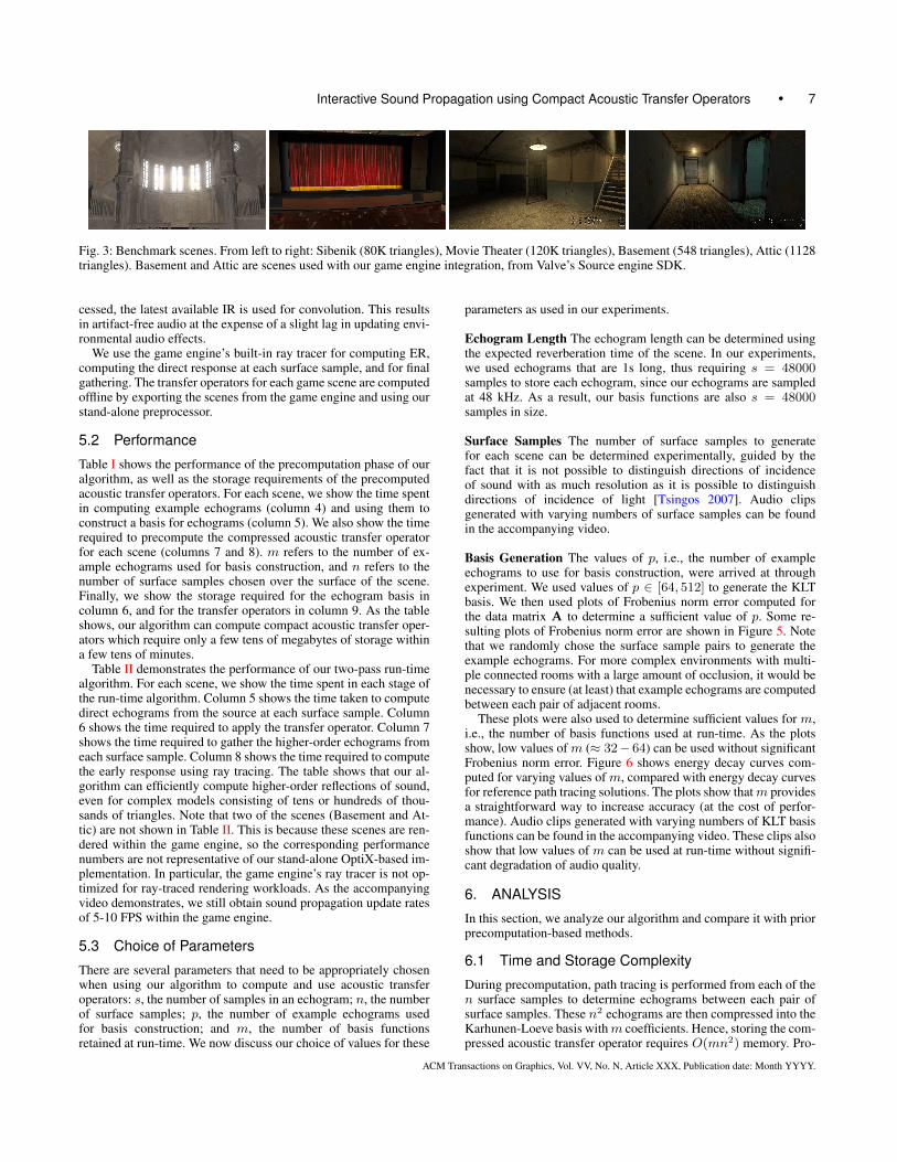
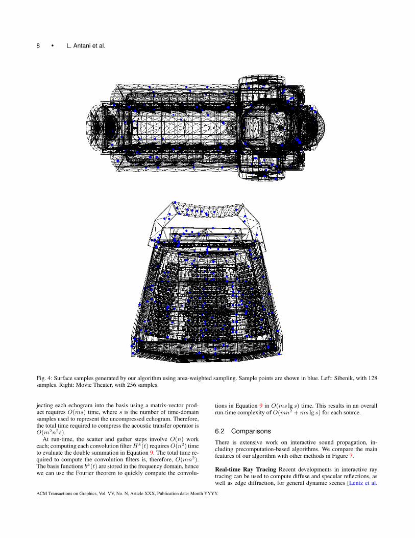
Our implementation is written in C++, compiled using MicrosoftVisual Studio 2010. We use Intel Math Kernel Library (MKL) forparallelization of linear algebra operations, and NVIDIA OptiXfor interactive ray tracing. All precomputation and run-time testswere performed on an Intel Core 2 Quad 2.83 GHz CPU with 4GBRAM and an NVIDIA GeForce GTX 480 GPU, running Windows7. Figure 3 shows the benchmark scenes used in our experiments.Figure 4 shows the surface samples generated for two of them.

Audio Processing Pipeline All of our echogram processing (dur-ing precomputation as well as at run-time) is performed in multiplefrequency bands. For efficiency, we perform processing in 3 fre-quency bands (20Hz–250Hz, 250Hz–2kHz and 2kHz-20kHz). A

similar approach has been adopted by Tsingos et al. [2004]. Moreaccuracy can be obtained by using more frequency bands; however,the processing costs scale linearly with the number of frequencybands.

Once the final echogram is computed for the listener, it is usedto estimate a pressure impulse response using standard techniques[Kuttruff 1993]. The estimated IR is then convolved with the dryaudio signal to compute the final sound heard at the listener.

For simplicity, we do not model the head-related transferfunction (HRTF) at the listener in our implementation; however,our algorithm can very easily incorporate HRTFs. This can beperformed during the final gathering stage of the radiance transferpass, and when tracing rays from the listener in the ray tracingpass. In both cases, the rays can be amplitude-panned into adistribution of directions, and the corresponding HRTF coefficientscan be included in the delays and attenuations applied for each ray.This would allow more accurate spatial reproduction of the soundfield at the listener. Similarly, while our algorithm can take intoaccount source directivity, we assume isotropic point sources in allour experiments for simplicity.

Game Engine Integration We have integrated our sound propa-gation system with Valve’s Source game engine, which has beenused by many popular video games, including Half-Life 2 andLeft 4 Dead. From within the game engine, we spawn a parallelthread which runs our sound propagation manager. The game en-gine generates sound events in response to gameplay or physicsevents such as footsteps, collisions, gunshots or speech. Whenevera sound event is triggered, we pass all relevant information (suchas the source position, orientation, and dry sound clip) to the soundpropagation manager.

The sound propagation manager computes the IR from eachsource to the listener (which is at the player’s position) and con-volves it with the corresponding sound signal before playback.Propagation and convolution occur asynchronously, in order to en-sure smooth, artifact-free audio. Note that propagation occurs at5-10 FPS, while audio needs to be output in real-time (44100 sam-ples per second). Therefore, IRs are updated independently of thestreaming audio processing pipeline. As each frame of audio is pro-



Fig. 3: Benchmark scenes. From left to right: Sibenik (80K triangles), Movie Theater (120K triangles), Basement (548 triangles), Attic (1128triangles). Basement and Attic are scenes used with our game engine integration, from Valve’s Source engine SDK.

cessed, the latest available IR is used for convolution. This resultsin artifact-free audio at the expense of a slight lag in updating envi-ronmental audio effects.

We use the game engine’s built-in ray tracer for computing ER,computing the direct response at each surface sample, and for finalgathering. The transfer operators for each game scene are computedoffline by exporting the scenes from the game engine and using ourstand-alone preprocessor.

5.2 Performance

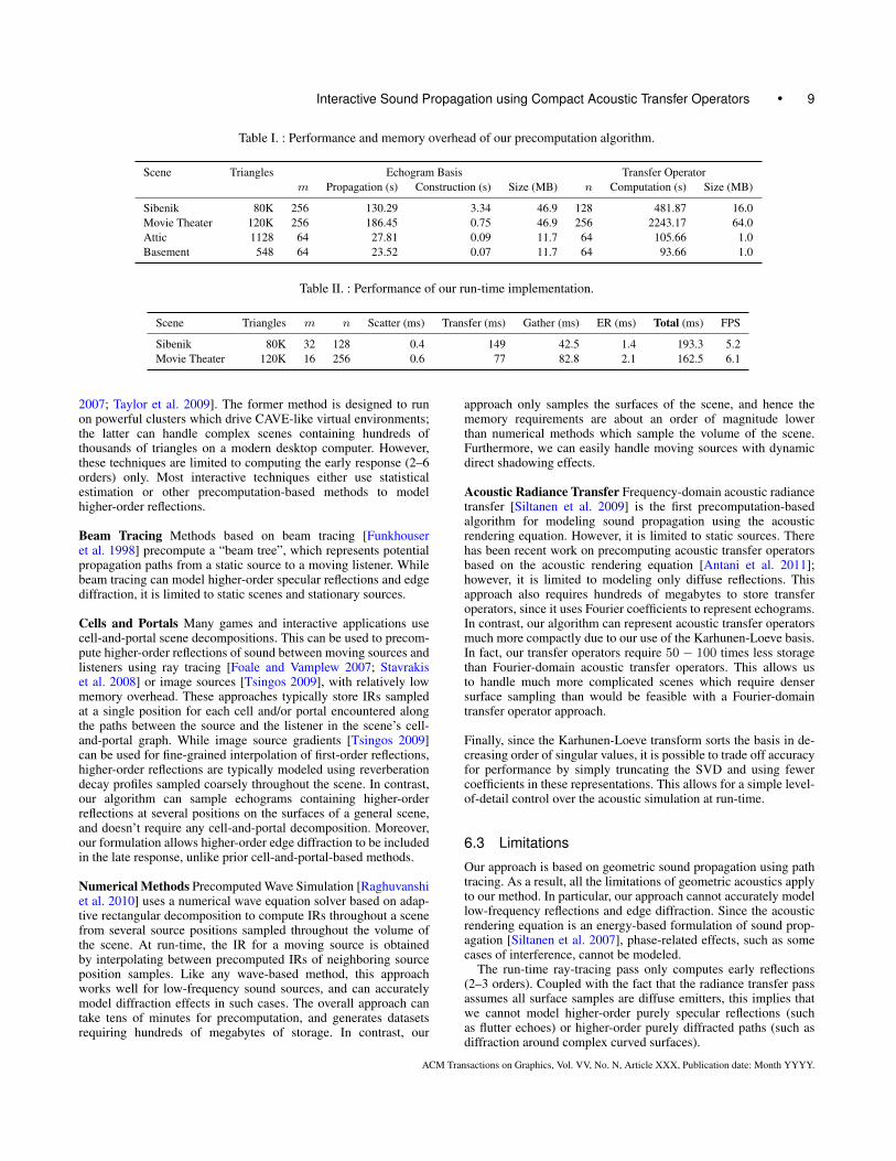
Table I shows the performance of the precomputation phase of ouralgorithm, as well as the storage requirements of the precomputedacoustic transfer operators. For each scene, we show the time spentin computing example echograms (column 4) and using them toconstruct a basis for echograms (column 5). We also show the timerequired to precompute the compressed acoustic transfer operatorfor each scene (columns 7 and 8). m refers to the number of ex-ample echograms used for basis construction, and n refers to thenumber of surface samples chosen over the surface of the scene.Finally, we show the storage required for the echogram basis incolumn 6, and for the transfer operators in column 9. As the tableshows, our algorithm can compute compact acoustic transfer oper-ators which require only a few tens of megabytes of storage withina few tens of minutes.

Table II demonstrates the performance of our two-pass run-timealgorithm. For each scene, we show the time spent in each stage ofthe run-time algorithm. Column 5 shows the time taken to computedirect echograms from the source at each surface sample. Column6 shows the time required to apply the transfer operator. Column 7shows the time required to gather the higher-order echograms fromeach surface sample. Column 8 shows the time required to computethe early response using ray tracing. The table shows that our al-gorithm can efficiently compute higher-order reflections of sound,even for complex models consisting of tens or hundreds of thou-sands of triangles. Note that two of the scenes (Basement and At-tic) are not shown in Table II. This is because these scenes are ren-dered within the game engine, so the corresponding performancenumbers are not representative of our stand-alone OptiX-based im-plementation. In particular, the game engine’s ray tracer is not op-timized for ray-traced rendering workloads. As the accompanyingvideo demonstrates, we still obtain sound propagation update ratesof 5-10 FPS within the game engine.

5.3 Choice of Parameters

There are several parameters that need to be appropriately chosenwhen using our algorithm to compute and use acoustic transferoperators: s, the number of samples in an echogram; n, the numberof surface samples; p, the number of example echograms usedfor basis construction; and m, the number of basis functionsretained at run-time. We now discuss our choice of values for these

parameters as used in our experiments.

Echogram Length The echogram length can be determined usingthe expected reverberation time of the scene. In our experiments,we used echograms that are 1s long, thus requiring s = 48000samples to store each echogram, since our echograms are sampledat 48 kHz. As a result, our basis functions are also s = 48000samples in size.

Surface Samples The number of surface samples to generatefor each scene can be determined experimentally, guided by thefact that it is not possible to distinguish directions of incidenceof sound with as much resolution as it is possible to distinguishdirections of incidence of light [Tsingos 2007]. Audio clipsgenerated with varying numbers of surface samples can be foundin the accompanying video.

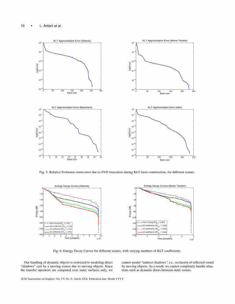
Basis Generation The values of p, i.e., the number of exampleechograms to use for basis construction, were arrived at throughexperiment. We used values of p ∈ [64, 512] to generate the KLTbasis. We then used plots of Frobenius norm error computed forthe data matrix A to determine a sufficient value of p. Some re-sulting plots of Frobenius norm error are shown in Figure 5. Notethat we randomly chose the surface sample pairs to generate theexample echograms. For more complex environments with multi-ple connected rooms with a large amount of occlusion, it would benecessary to ensure (at least) that example echograms are computedbetween each pair of adjacent rooms.

These plots were also used to determine sufficient values for m,i.e., the number of basis functions used at run-time. As the plotsshow, low values of m (≈ 32− 64) can be used without significantFrobenius norm error. Figure 6 shows energy decay curves com-puted for varying values of m, compared with energy decay curvesfor reference path tracing solutions. The plots show thatm providesa straightforward way to increase accuracy (at the cost of perfor-mance). Audio clips generated with varying numbers of KLT basisfunctions can be found in the accompanying video. These clips alsoshow that low values of m can be used at run-time without signifi-cant degradation of audio quality.

6. ANALYSIS

In this section, we analyze our algorithm and compare it with priorprecomputation-based methods.

6.1 Time and Storage Complexity

During precomputation, path tracing is performed from each of then surface samples to determine echograms between each pair ofsurface samples. These n2 echograms are then compressed into theKarhunen-Loeve basis withm coefficients. Hence, storing the com-pressed acoustic transfer operator requires O(mn2) memory. Pro-



Fig. 4: Surface samples generated by our algorithm using area-weighted sampling. Sample points are shown in blue. Left: Sibenik, with 128samples. Right: Movie Theater, with 256 samples.

jecting each echogram into the basis using a matrix-vector prod-uct requires O(ms) time, where s is the number of time-domainsamples used to represent the uncompressed echogram. Therefore,the total time required to compress the acoustic transfer operator isO(m2n2s).

At run-time, the scatter and gather steps involve O(n) workeach; computing each convolution filterHk(t) requiresO(n2) timeto evaluate the double summation in Equation 9. The total time re-quired to compute the convolution filters is, therefore, O(mn2).The basis functions bk(t) are stored in the frequency domain, hencewe can use the Fourier theorem to quickly compute the convolu-

tions in Equation 9 in O(ms lg s) time. This results in an overallrun-time complexity of O(mn2 +ms lg s) for each source.

6.2 Comparisons

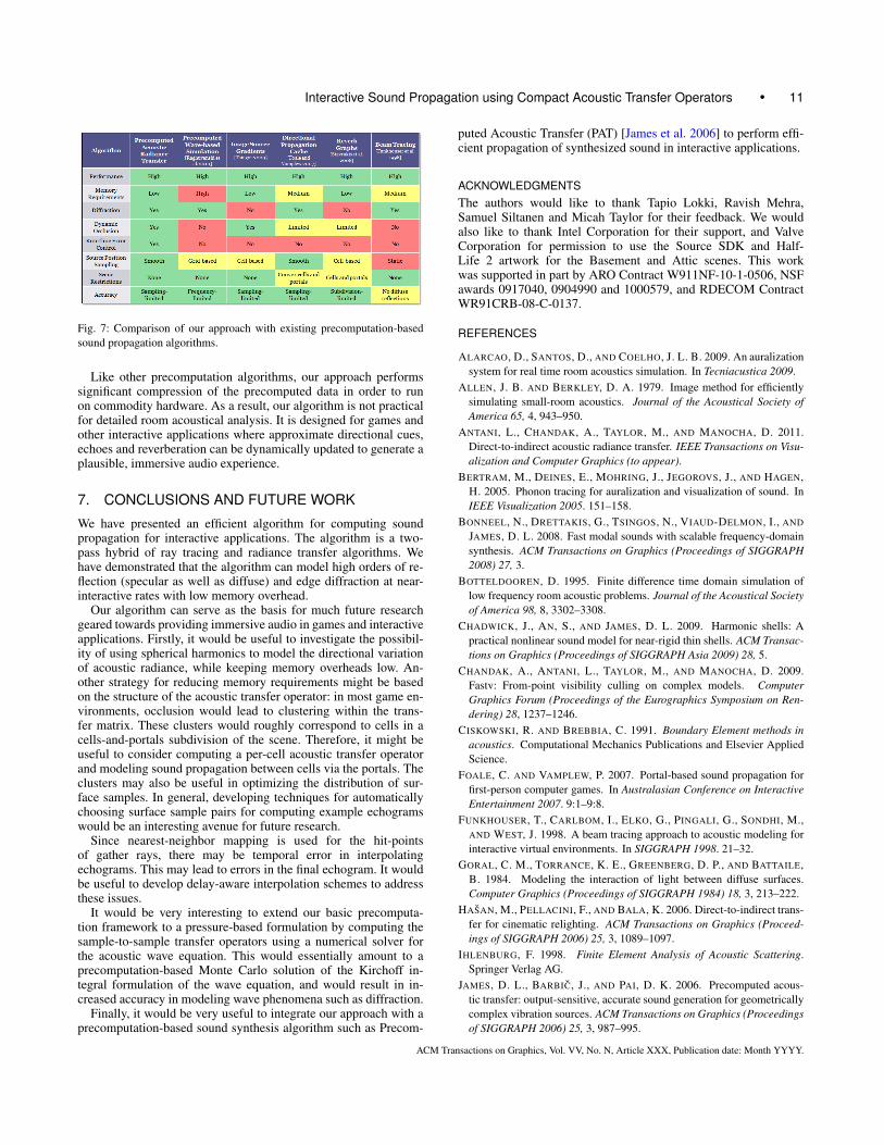
There is extensive work on interactive sound propagation, in-cluding precomputation-based algorithms. We compare the mainfeatures of our algorithm with other methods in Figure 7.

Real-time Ray Tracing Recent developments in interactive raytracing can be used to compute diffuse and specular reflections, aswell as edge diffraction, for general dynamic scenes [Lentz et al.



Table I. : Performance and memory overhead of our precomputation algorithm.

Scene Triangles Echogram Basis Transfer Operatorm Propagation (s) Construction (s) Size (MB) n Computation (s) Size (MB)

Sibenik 80K 256 130.29 3.34 46.9 128 481.87 16.0Movie Theater 120K 256 186.45 0.75 46.9 256 2243.17 64.0Attic 1128 64 27.81 0.09 11.7 64 105.66 1.0Basement 548 64 23.52 0.07 11.7 64 93.66 1.0

Table II. : Performance of our run-time implementation.

Scene Triangles m n Scatter (ms) Transfer (ms) Gather (ms) ER (ms) Total (ms) FPS

Sibenik 80K 32 128 0.4 149 42.5 1.4 193.3 5.2Movie Theater 120K 16 256 0.6 77 82.8 2.1 162.5 6.1

2007; Taylor et al. 2009]. The former method is designed to runon powerful clusters which drive CAVE-like virtual environments;the latter can handle complex scenes containing hundreds ofthousands of triangles on a modern desktop computer. However,these techniques are limited to computing the early response (2–6orders) only. Most interactive techniques either use statisticalestimation or other precomputation-based methods to modelhigher-order reflections.

Beam Tracing Methods based on beam tracing [Funkhouseret al. 1998] precompute a “beam tree”, which represents potentialpropagation paths from a static source to a moving listener. Whilebeam tracing can model higher-order specular reflections and edgediffraction, it is limited to static scenes and stationary sources.

Cells and Portals Many games and interactive applications usecell-and-portal scene decompositions. This can be used to precom-pute higher-order reflections of sound between moving sources andlisteners using ray tracing [Foale and Vamplew 2007; Stavrakiset al. 2008] or image sources [Tsingos 2009], with relatively lowmemory overhead. These approaches typically store IRs sampledat a single position for each cell and/or portal encountered alongthe paths between the source and the listener in the scene’s cell-and-portal graph. While image source gradients [Tsingos 2009]can be used for fine-grained interpolation of first-order reflections,higher-order reflections are typically modeled using reverberationdecay profiles sampled coarsely throughout the scene. In contrast,our algorithm can sample echograms containing higher-orderreflections at several positions on the surfaces of a general scene,and doesn’t require any cell-and-portal decomposition. Moreover,our formulation allows higher-order edge diffraction to be includedin the late response, unlike prior cell-and-portal-based methods.

Numerical Methods Precomputed Wave Simulation [Raghuvanshiet al. 2010] uses a numerical wave equation solver based on adap-tive rectangular decomposition to compute IRs throughout a scenefrom several source positions sampled throughout the volume ofthe scene. At run-time, the IR for a moving source is obtainedby interpolating between precomputed IRs of neighboring sourceposition samples. Like any wave-based method, this approachworks well for low-frequency sound sources, and can accuratelymodel diffraction effects in such cases. The overall approach cantake tens of minutes for precomputation, and generates datasetsrequiring hundreds of megabytes of storage. In contrast, our

approach only samples the surfaces of the scene, and hence thememory requirements are about an order of magnitude lowerthan numerical methods which sample the volume of the scene.Furthermore, we can easily handle moving sources with dynamicdirect shadowing effects.

Acoustic Radiance Transfer Frequency-domain acoustic radiancetransfer [Siltanen et al. 2009] is the first precomputation-basedalgorithm for modeling sound propagation using the acousticrendering equation. However, it is limited to static sources. Therehas been recent work on precomputing acoustic transfer operatorsbased on the acoustic rendering equation [Antani et al. 2011];however, it is limited to modeling only diffuse reflections. Thisapproach also requires hundreds of megabytes to store transferoperators, since it uses Fourier coefficients to represent echograms.In contrast, our algorithm can represent acoustic transfer operatorsmuch more compactly due to our use of the Karhunen-Loeve basis.In fact, our transfer operators require 50 − 100 times less storagethan Fourier-domain acoustic transfer operators. This allows usto handle much more complicated scenes which require densersurface sampling than would be feasible with a Fourier-domaintransfer operator approach.

Finally, since the Karhunen-Loeve transform sorts the basis in de-creasing order of singular values, it is possible to trade off accuracyfor performance by simply truncating the SVD and using fewercoefficients in these representations. This allows for a simple level-of-detail control over the acoustic simulation at run-time.

6.3 Limitations

Our approach is based on geometric sound propagation using pathtracing. As a result, all the limitations of geometric acoustics applyto our method. In particular, our approach cannot accurately modellow-frequency reflections and edge diffraction. Since the acousticrendering equation is an energy-based formulation of sound prop-agation [Siltanen et al. 2007], phase-related effects, such as somecases of interference, cannot be modeled.

The run-time ray-tracing pass only computes early reflections(2–3 orders). Coupled with the fact that the radiance transfer passassumes all surface samples are diffuse emitters, this implies thatwe cannot model higher-order purely specular reflections (suchas flutter echoes) or higher-order purely diffracted paths (such asdiffraction around complex curved surfaces).



0 50 100 150 200 250 30010−25

10−20

10−15

10−10

10−5

100

Basis size

log(

Err

or)

KLT Approximation Error (Sibenik)

0 50 100 150 200 25010−50

10−40

10−30

10−20

10−10

100

Basis size

log(

Err

or)

KLT Approximation Error (Movie Theater)

0 5 10 15 20 25 30 35 40 4510−40

10−35

10−30

10−25

10−20

10−15

10−10

10−5

100

Basis size

log(

Err

or)

KLT Approximation Error (Basement)

0 50 100 150 200 25010−40

10−35

10−30

10−25

10−20

10−15

10−10

10−5

100

Basis size

log(

Err

or)

KLT Approximation Error (Attic)

Fig. 5: Relative Frobenius norm error due to SVD truncation during KLT basis construction, for different scenes.

0 1 2 3 4 5 6 7 8 9 10

x 104

−160

−140

−120

−100

−80

−60

−40

−20

0

Time (samples)

Ene

rgy

(dB

)

Energy Decay Curves (Sibenik)

Path Tracing (RT60

= 1.37s)

256 coefficients (RT60

= 1.12s)


= 1.10s)


= 1.09s)

0 1 2 3 4 5

x 104

−160

−140

−120

−100

−80

−60

−40

−20

0

Time (samples)

Ene

rgy

(dB

)

Energy Decay Curves (Movie Theater)

Path Tracing (RT60

= 1.45s)


= 1.15s)


= 1.03s)


= 1.02s)

Fig. 6: Energy Decay Curves for different scenes, with varying numbers of KLT coefficients.

Our handling of dynamic objects is restricted to modeling direct“shadows” cast by a moving source due to moving objects. Sincethe transfer operators are computed over static surfaces only, we

cannot model “indirect shadows”, i.e., occlusion of reflected soundby moving objects. As a result, we cannot completely handle situa-tions such as dynamic doors between static rooms.



Fig. 7: Comparison of our approach with existing precomputation-basedsound propagation algorithms.

Like other precomputation algorithms, our approach performssignificant compression of the precomputed data in order to runon commodity hardware. As a result, our algorithm is not practicalfor detailed room acoustical analysis. It is designed for games andother interactive applications where approximate directional cues,echoes and reverberation can be dynamically updated to generate aplausible, immersive audio experience.

7. CONCLUSIONS AND FUTURE WORK

We have presented an efficient algorithm for computing soundpropagation for interactive applications. The algorithm is a two-pass hybrid of ray tracing and radiance transfer algorithms. Wehave demonstrated that the algorithm can model high orders of re-flection (specular as well as diffuse) and edge diffraction at near-interactive rates with low memory overhead.

Our algorithm can serve as the basis for much future researchgeared towards providing immersive audio in games and interactiveapplications. Firstly, it would be useful to investigate the possibil-ity of using spherical harmonics to model the directional variationof acoustic radiance, while keeping memory overheads low. An-other strategy for reducing memory requirements might be basedon the structure of the acoustic transfer operator: in most game en-vironments, occlusion would lead to clustering within the trans-fer matrix. These clusters would roughly correspond to cells in acells-and-portals subdivision of the scene. Therefore, it might beuseful to consider computing a per-cell acoustic transfer operatorand modeling sound propagation between cells via the portals. Theclusters may also be useful in optimizing the distribution of sur-face samples. In general, developing techniques for automaticallychoosing surface sample pairs for computing example echogramswould be an interesting avenue for future research.

Since nearest-neighbor mapping is used for the hit-pointsof gather rays, there may be temporal error in interpolatingechograms. This may lead to errors in the final echogram. It wouldbe useful to develop delay-aware interpolation schemes to addressthese issues.

It would be very interesting to extend our basic precomputa-tion framework to a pressure-based formulation by computing thesample-to-sample transfer operators using a numerical solver forthe acoustic wave equation. This would essentially amount to aprecomputation-based Monte Carlo solution of the Kirchoff in-tegral formulation of the wave equation, and would result in in-creased accuracy in modeling wave phenomena such as diffraction.

Finally, it would be very useful to integrate our approach with aprecomputation-based sound synthesis algorithm such as Precom-

puted Acoustic Transfer (PAT) [James et al. 2006] to perform effi-cient propagation of synthesized sound in interactive applications.

ACKNOWLEDGMENTSThe authors would like to thank Tapio Lokki, Ravish Mehra,Samuel Siltanen and Micah Taylor for their feedback. We wouldalso like to thank Intel Corporation for their support, and ValveCorporation for permission to use the Source SDK and Half-Life 2 artwork for the Basement and Attic scenes. This workwas supported in part by ARO Contract W911NF-10-1-0506, NSFawards 0917040, 0904990 and 1000579, and RDECOM ContractWR91CRB-08-C-0137.

REFERENCES

ALARCAO, D., SANTOS, D., AND COELHO, J. L. B. 2009. An auralizationsystem for real time room acoustics simulation. In Tecniacustica 2009.

ALLEN, J. B. AND BERKLEY, D. A. 1979. Image method for efficientlysimulating small-room acoustics. Journal of the Acoustical Society ofAmerica 65, 4, 943–950.

ANTANI, L., CHANDAK, A., TAYLOR, M., AND MANOCHA, D. 2011.Direct-to-indirect acoustic radiance transfer. IEEE Transactions on Visu-alization and Computer Graphics (to appear).

BERTRAM, M., DEINES, E., MOHRING, J., JEGOROVS, J., AND HAGEN,H. 2005. Phonon tracing for auralization and visualization of sound. InIEEE Visualization 2005. 151–158.

BONNEEL, N., DRETTAKIS, G., TSINGOS, N., VIAUD-DELMON, I., AND

JAMES, D. L. 2008. Fast modal sounds with scalable frequency-domainsynthesis. ACM Transactions on Graphics (Proceedings of SIGGRAPH2008) 27, 3.

BOTTELDOOREN, D. 1995. Finite difference time domain simulation oflow frequency room acoustic problems. Journal of the Acoustical Societyof America 98, 8, 3302–3308.

CHADWICK, J., AN, S., AND JAMES, D. L. 2009. Harmonic shells: Apractical nonlinear sound model for near-rigid thin shells. ACM Transac-tions on Graphics (Proceedings of SIGGRAPH Asia 2009) 28, 5.

CHANDAK, A., ANTANI, L., TAYLOR, M., AND MANOCHA, D. 2009.Fastv: From-point visibility culling on complex models. ComputerGraphics Forum (Proceedings of the Eurographics Symposium on Ren-dering) 28, 1237–1246.

CISKOWSKI, R. AND BREBBIA, C. 1991. Boundary Element methods inacoustics. Computational Mechanics Publications and Elsevier AppliedScience.

FOALE, C. AND VAMPLEW, P. 2007. Portal-based sound propagation forfirst-person computer games. In Australasian Conference on InteractiveEntertainment 2007. 9:1–9:8.

FUNKHOUSER, T., CARLBOM, I., ELKO, G., PINGALI, G., SONDHI, M.,AND WEST, J. 1998. A beam tracing approach to acoustic modeling forinteractive virtual environments. In SIGGRAPH 1998. 21–32.

GORAL, C. M., TORRANCE, K. E., GREENBERG, D. P., AND BATTAILE,B. 1984. Modeling the interaction of light between diffuse surfaces.Computer Graphics (Proceedings of SIGGRAPH 1984) 18, 3, 213–222.

HASAN, M., PELLACINI, F., AND BALA, K. 2006. Direct-to-indirect trans-fer for cinematic relighting. ACM Transactions on Graphics (Proceed-ings of SIGGRAPH 2006) 25, 3, 1089–1097.

IHLENBURG, F. 1998. Finite Element Analysis of Acoustic Scattering.Springer Verlag AG.

JAMES, D. L., BARBIC, J., AND PAI, D. K. 2006. Precomputed acous-tic transfer: output-sensitive, accurate sound generation for geometricallycomplex vibration sources. ACM Transactions on Graphics (Proceedingsof SIGGRAPH 2006) 25, 3, 987–995.



KAJIYA, J. T. 1986. The rendering equation. Computer Graphics (Pro-ceedings of SIGGRAPH 1986) 20, 4, 143–150.

KAPRALOS, B., JENKIN, M., AND MILIOS, E. 2004. Sonel mapping:acoustic modeling utilizing an acoustic version of photon mapping. InIEEE International Workshop on Haptics Audio Visual Environments andtheir Applications 2004.

KRISTENSEN, A. W., AKENINE-MOLLER, T., AND JENSEN, H. W. 2005.Precomputed local radiance transfer for real-time lighting design. ACMTransactions on Graphics (Proceedings of SIGGRAPH 2005) 24, 3,1208–1215.

KUTTRUFF, H. 1991. Room Acoustics. Elsevier Science Publishing Ltd.KUTTRUFF, H. 1995. A simple iteration scheme for the computation of

decay constants in enclosures with diffusely reflecting boundaries. TheJournal of the Acoustical Society of America 98, 1, 288–293.

KUTTRUFF, H. K. 1993. Auralization of Impulse Responses Modeled onthe Basis of Ray-Tracing Results. Journal of the Audio Engineering So-ciety 41, 11 (November), 876–880.

LAINE, S., SILTANEN, S., LOKKI, T., AND SAVIOJA, L. 2009. Acceleratedbeam tracing algorithm. Applied Acoustics 70, 1, 172–181.

LEHTINEN, J., ZWICKER, M., TURQUIN, E., KONTKANEN, J., DURAND,F., SILLION, F. X., AND AILA, T. 2008. A meshless hierarchical repre-sentation for light transport. ACM Transactions on Graphics (Proceed-ings of SIGGRAPH 2008) 27, 3, 1–9.

LENTZ, T., SCHROEDER, D., VORLANDER, M., AND ASSENMACHER, I.2007. Virtual reality system with integrated sound field simulation andreproduction. EURASIP Journal of Applied Signal Processing 2007, 1.

LOEVE, M. 1978. Probability Theory Vol. II. Springer-Verlag.MOECK, T., BONNEEL, N., TSINGOS, N., DRETTAKIS, G., VIAUD-

DELMON, I., AND ALOZA, D. 2007. Progressive perceptual audio ren-dering of complex scenes. In ACM SIGGRAPH Symposium on Interactive3D Graphics and Games.

NOSAL, E.-M., HODGSON, M., AND ASHDOWN, I. 2004. Improved al-gorithms and methods for room sound-field prediction by acoustical ra-diosity in arbitrary polyhedral rooms. Journal of the Acoustical Societyof America 116, 2, 970–980.

RAGHUVANSHI, N. AND LIN, M. C. 2006. Interactive sound synthesis forlarge scale environments. In Symposium on Interactive 3D Graphics andGames.

RAGHUVANSHI, N., NARAIN, R., AND LIN, M. C. 2009. Efficient andaccurate sound propagation using adaptive rectangular decomposition.IEEE Transactions on Visualization and Computer Graphics 15, 789–801.

RAGHUVANSHI, N., SNYDER, J., MEHRA, R., LIN, M., AND GOVIN-DARAJU, N. 2010. Precomputed wave simulation for real-time soundpropagation of dynamic sources in complex scenes. ACM Transactionson Graphics (Proceedings of SIGGRAPH 2010) 29, 4, 68:1 – 68:11.

SAVIOJA, L., HUOPANIEMI, J., LOKKI, T., AND VAANANEN, R. 1999.Creating interactive virtual acoustic environments. Journal of the AudioEngineering Society 47, 9, 675–705.

SAVIOJA, L., RINNE, T., AND TAKALA, T. 1994. Simulation of roomacoustics with a 3-D finite difference mesh. In International ComputerMusic Conference. 463–466.

SILTANEN, S., LOKKI, T., KIMINKI, S., AND SAVIOJA, L. 2007. Theroom acoustic rendering equation. Journal of the Acoustical Society ofAmerica 122, 3, 1624–1635.

SILTANEN, S., LOKKI, T., AND SAVIOJA, L. 2009. Frequency domainacoustic radiance transfer for real-time auralization. Acta Acustica unitedwith Acustica 95, 106–117.

SLOAN, P.-P., KAUTZ, J., AND SNYDER, J. 2002. Precomputed radiancetransfer for real-time rendering in dynamic, low-frequency lighting envi-

ronments. ACM Transactions on Graphics (Proceedings of SIGGRAPH2002) 21, 3, 527–536.

STAVRAKIS, E., TSINGOS, N., AND CALAMIA, P. 2008. Topologicalsound propagation with reverberation graphs. Acta Acustica united withAcustica.

STEPHENSON, U. M. 2010. An analytically derived sound particle diffrac-tion model. Acta Acustica united with Acustica 96, 1051–1068.

STEPHENSON, U. M. AND SVENSSON, U. P. 2007. An improved ener-getic approach to diffraction based on the unvertainty principle. 19thInternational Congress on Acoustics (ICA).

SUMMERS, J. E., TORRES, R. R., AND SHIMIZU, Y. 2004. Statistical-acoustics models of energy decay in systems of coupled rooms and theirrelation to geometrical acoustics. Journal of the Acoustical Society ofAmerica 116, 2, 958–969.

SVENSSON, U. P., FRED, R. I., AND VANDERKOOY, J. 1999. An analyticsecondary source model of edge diffraction impulse responses. Journalof the Acoustical Society of America 106, 2331–2344.

TAYLOR, M. T., CHANDAK, A., ANTANI, L., AND MANOCHA, D. 2009.Resound: interactive sound rendering for dynamic virtual environments.In ACM Multimedia 2009. 271–280.

TSINGOS, N. 2007. Perceptually-based auralization. In InternationalCongress on Acoustics.

TSINGOS, N. 2009. Precomputing geometry-based reverberation effectsfor games. In Audio Engineering Society Conference: Audio for Games.

TSINGOS, N., FUNKHOUSER, T., NGAN, A., AND CARLBOM, I. 2001.Modeling acoustics in virtual environments using the uniform theory ofdiffraction. In SIGGRAPH 2001. 545–552.

TSINGOS, N., GALLO, E., AND DRETTAKIS, G. 2004. Perceptual au-dio rendering of complex virtual environments. ACM Transactions onGraphics (Proceedings of SIGGRAPH 2004) 23, 3.

TSINGOS, N. AND GASCUEL, J.-D. 1997. A general model for the sim-ulation of room acoustics based on hierachical radiosity. In ACM SIG-GRAPH 97 Visual Proceedings.

WALLACE, J. R., COHEN, M. F., AND GREENBERG, D. P. 1987. Atwo-pass solution to the rendering equation: A synthesis of ray tracingand radiosity methods. Computer Graphics (Proceedings of SIGGRAPH1987) 21, 4, 311–320.

WANG, YE; VILERMO, M. 2003. Modified discrete cosine transform:Its implications for audio coding and error concealment. J. Audio Eng.Soc 51, 1/2, 52–61.


Documents

Interactive Sound Propagation using Compact Acoustic ...gamma.cs.unc.edu/CATR/part.pdf · transfer, higher-order reﬂections, interactive applications 1. INTRODUCTION Realistic sound