Interactive Shape Interpolation through Controllable Dynamic Deformation

Jin Huang∗ Yiying Tong† Kun Zhou∗ Hujun Bao∗ Mathieu Desbrun‡

∗Zhejiang University †Michigan State University ‡Caltech

Figure 1: Our shape interpolation can interactively provide a dynamic motion between two poses. Here, the interpolation is demonstrated on an elephant

model, the first pose being with the trunk down (leftmost) and the final pose (the rest state) being with the trunk up in the air (rightmost). Although many

dynamical coefficients can be interactively edited, we show in the top row a direct vibration-free interpolation generated (µ = −1 and η = −1), while the

bottom row demonstrates the effect of adding low frequency to the motion: the trunk and ears now dynamically deform throughout the pose interpolation.

Abstract

In this paper, we introduce an interactive approach to generatephysically-based shape interpolation between two poses. We com-bine an extension of modal analysis to large deformation and a Pois-son reconstruction from deformation gradient to offer physically-plausible dynamics at interactive rates. Our method also provides arich set of intuitive editing tools with real-time feedback, includingcontrol over vibration frequencies, amplitudes, and damping of theresulting interpolation sequence. We demonstrate the versatility ofour approach through a series of complex dynamic shape interpola-tions.

Keywords: Deformation Gradient, Shape Interpolation, Space-Time Constraints

1 Introduction

In computer animation of characters or deformable objects, inter-polating between two given poses (key frames) of a same mesh isa ubiquitous task. One must not only produce visually-pleasingdeformations between shapes, but also create complex dynamic id-iosyncracies along the way to increase realism and visual impact.Offering an easy-to-use, interactive framework for a dynamic shapeinterpolation is currently, however, considered fastidious.

1.1 Problem Statement

In this paper, we will deal with 3D objects, each represented asa simplicial complex (x, C), where C encodes the connectivity ofthe tetrahedral mesh and x = (xt

1, · · · , xtn)t ∈ R3n denotes the

shape, i.e., the set of positions of the mesh vertices. We assumethat an object (r, C), where r is its rest shape, is provided by theuser, along with two poses xA, xB of this 3D object. We wish toevaluate a physically-based shape deformation x(t), with t∈ [0, T ],such that: {

x(0) = xA

x(T ) = xB ,

while offering intuitive and interactive control over the dynamicsthroughout the interpolation sequence.

1.2 Previous Work

Pose interpolation has been investigated in a number of contexts.We briefly review the main approaches next.

Purely Geometric Interpolation Shape interpolation methods pro-vide fast and reasonable inbetweening of two given geometricshapes, albeit without control over dynamical effects. For example,“as-rigid-as-possible” shape interpolation establishes compatibletriangulation of 2D or 3D shapes, and creates per-simplex interpo-lations of the corresponding simplices based on a geometric decom-position of the transformation matrix into a rotation and a stretchingmatrix. The final vertex paths are computed through a global bestfit of these per-simplex transformations [Alexa et al. 2000]. Geo-metric modeling in “shape space” is another purely geometric ap-proach to shape interpolation, where a notion of geodesics in shapespace is used to provide an as-isometric-as-possible path betweentwo poses [Kilian et al. 2007].

Physically-based Interpolation If material properties are known,one can theoretically solve for the optimal deformation betweentwo given poses of an elastic object through space-time con-straints and/or optimal control methods [Witkin and Kass 1988;Popovic et al. 2000]. However, nonlinearities induced by the

laws of physics render these approaches dramatically slower thanpurely geometric methods for complex objects (if not intractable).More recently, an approach based on coarse and meshless mod-eling [Adams et al. 2008] of deformable shapes was introduced toproduce smooth interpolations at interactive frame rates through aminimization of rigidity and volume-preservation energies. How-ever, the results are visually similar to purely geometric meth-ods, producing little to no vibrations due to the choice of mostlygeometrically-motivated energies. Optimal control was also ex-plored lately to adjust a motion to a desired trajectory in real-time[Barbic and Popovic 2008], but it did not address the challeng-ing problem of getting the initial trajectory connecting the input keyframes at interactive rates.

Modal Analysis Although not directly applicable to the prob-lem of pose interpolation per se, a particularly efficient and nat-ural way to model physical behavior is through modal analy-sis [Pentland and Williams 1989; James and Pai 2002], which de-composes the space of deformations into a set of vibrationmodes. Note that linear modal analysis is only physically validfor small perturbation around the pose over which spectral anal-ysis of the stiffness and mass matrices is performed. How-ever, a corotational method (“Modal Warping”) was recently pro-posed to gracefully extend the original approach to large defor-mations [Choi and Ko 2005], at the price of an approximate timeintegration to compute positions. Unfortunately, modal analysishas been used primarily for forward physical simulation instead ofinterpolation between given key frames. Recent model reductionmethods [Feng et al. 2008; Popa et al. 2009] are purely data-driven,with no explicit modeling or control of dynamic properties, such asmass, damping, frequency etc. Closer to our concern is a recentapproach coined Wiggly Splines [Kass and Anderson 2008], whichprovides a link between traditional animation splines and vibrationmodes. With their framework, assuming that vibration modes ofan object are known (via either procedural or example-based meth-ods), an animator can design a motion from one pose to anothercontaining intentional vibrations whose frequency, damping, andrelative phase can be tweaked as desired for cinematic effect. Whilethis method offers intuitive control of the deformation and its dy-namics, the linear space of deformations that the authors restrict theapproach to seems mostly amenable, as is, to wiggly motions.

1.3 Rationale and Contributions

We depart from previous methods by proposing an approach thatdraws both on physically-based (in particular, through spectral mo-tion decomposition) and geometric methods (through a geometricdecomposition of eigenmodes). Building upon the equations of lin-ear elasticity that govern small deformations, our hybrid techniquetreats linear deformation modes as tangent vectors in a rotation-strain space, which describes the deformed object through its de-formation gradient field represented as the product of a local rota-tion and a material stretch tensor. Linear combinations of modes inthis new representation produce physically-plausible large elasticdeformations akin to those in Modal Warping. However, our ap-proach further allows a simple map between the shape change intime, and analytic solutions of the time evolution of modes. As aresult, we contribute to the problem of elastic shape deformationby proposing an interactive alternative to Space-Time Constraintsas efficient as purely geometric methods, yet offering a rich set ofcontrols over the dynamics of interpolation: any pair of poses canbe interpolated, while the frequency, amplitude, and damping ofvibration modes can be intuitively and interactively edited.

1.4 Algorithm Overview

Our algorithm is composed of a pre-computation part and a runtimecomputation part.

• Pre-computation: Given a tetrahedron mesh in its rest shape, we

compute the vibration modes W through classical Modal Analy-

sis. Then we convert them into a basis W in rotation-strain space(Section 2.2), capable of representing large deformation.

• Runtime computation: Key frames x(0), x(T ) are also con-verted into rotation-strain space as x(0), x(T ) (Section 2.1).Their modal coordinates z(0), z(T ) are then computed through

the relation Wz(t) = x(t). With (optional) user controls, weinterpolate z(0) and z(T ) according to the free vibration mo-tion equation with optimal frequency and damping parameters(Section 2.3), and finally reconstruct the shape through Poissonreconstruction (Section 2.1).

2 Dynamic Shape Interpolation

Our approach consists in a succession of a few simple steps, someperformed offline before any user-interaction, and some performedat runtime to allow for interactive design of a dynamic shape inter-polation between two poses. This section elaborates on each indi-vidual component one by one, before presenting the overall algo-rithm in Section 2.4.

2.1 Rotation-Strain Coordinates

To help us deal with large deformation, we introduce rotation-straincoordinates based on polar decomposition of the deformation gra-dient of a pose. Given a shape vector x, its deformation gradi-ent with respect to the rest shape r is computed as m=Gx (one3x3 matrix per tet), where G is the commonly-used discrete gra-dient operator corresponding to the continuous gradient operator∇ with respect to r through linear finite elements [Bathe 1995].For each tet Ti, we further decompose mi = (Gx)i using po-lar decomposition [Bertram 2005] into the product of a rotationRi and a symmetric tensor Id + Si (where Id is the identity ma-trix, and Si is the Biot strain tensor [Bertram 2005]). Similarlyto [Der et al. 2006], we finally apply the logarithm function to therotation matrix, thus decomposing the deformation gradient mi pertet into a pair [log(Ri), Si]. The array x := {{log(Ri)}i, {Si}i}(where the index i goes through every tet) thus encodes the defor-mation gradient for the whole shape x, and forms what we willabusively refer to as rotation-strain coordinates for simplicity. Wewill denote by T (·) the map between the Euclidean coordinates ofshape x and the rotation-strain coordinates x := T (x). Note thatthis map is non-linear, but simple to compute through local polardecomposition of the deformation gradient. Note also that by defi-nition, the rest shape r has null rotation-strain coordinates: r = 0.

Finally, one can recover the shape x from the rotation-strain co-ordinates x={{log(Ri)}i, {Si}i} through a pseudo-inverse mapsT −1(x), defined through exponentials of matrices and a simple lin-ear solve:

T −1(x)=arg minx

∑

tet Ti

‖(Gx)i−[exp(log(Ri))(Id+Si)]‖2

subject to:1

n

n∑

i=1

xi = c,(1)

where the position constraint is used to remove the translation in-variance of our representation, and ‖·‖ denotes the Frobenius normof matrices. The position c can, e.g., be set to the linear interpola-tion of the two barycenters of boundary shapes, or set to follow aparabola if the object is supposed to be free-falling. Note that thisshape recovery from our coordinates is essentially a 3D Poissonreconstruction, as x derives from the deformation gradient field.Simply adding the (rescaled) norm of the constraint as a penaltyterm to the target function, we solve the unconstrained least squareproblem with the package UMFPACK [Davis 2004].

2.2 Non-linear Vibration Modes

As we now detail, the rotation-strain space we defined is a par-ticularly convenient way to extend linear modal analysis (that wereview briefly first) and produce analytical expressions of large vi-brations.

2.2.1 Modal Analysis Overview

When considering small deformations around the rest shape, lin-ear elasticity is a good alternative to the full treatment of nonlineardynamics. Equations of motion are written in terms of the displace-ment field u=x − r between a current shape x and the rest state rthrough:

Ku + Du + Mu = 0 (2)

where K is the classical linear finite element stiffness matrix (theHessian of the quadratic potential energy of the deformable body),while M is the lumped mass matrix (see [Bathe 1995] for details).Matrix D describes the commonly-used Raleigh damping, definedas D=αKK+αMM , where αK and αM are damping parameters.

Further simplifications can be exploited through Modal Analy-sis [Pentland and Williams 1989; Hauser et al. 2003], an approachthat makes use of the solutions of the generalized eigenproblem:

Ky = λ2My, (3)

which are vibration (eigen)modes Wi of (eigen)frequency λi rep-resenting the natural characteristic displacements that the elasticobject can undergo. After assembling the modes in a modal dis-placement matrix W = (W1 W2 . . . Wn) and the eigenvalues in adiagonal modal frequency matrix Λ = diag(λ2

1, λ22, . . . , λ

2n), one

can verify that the modal displacement matrix W diagonalizes bothstiffness and mass matrices:

W tKW = Λ W tMW = Id.

Consequently, if we decompose a time-varying deformation u(t)into its modal components through

u(t) = Wz(t)

where z(t) stores the modal coordinates (representing the “magni-tudes” of all the eigenmodes), then Eq. (2) can be written as:

Λ z + (αKΛ + αM Id) z + z = 0, (4)

Notice that the dynamics of each eigenmode can now be computedindependently since Λ is diagonal. Finally, the shape trajectory x(t)can easily be recombined by linear superposition of each modalmagnitude through x(t)=r+Wz(t) to get the resulting elastic mo-tion. For efficiency, one may only keep the modes corresponding tolow frequencies as this drastically reduces the amount of computa-tions necessary to generate a realistic motion.

2.2.2 Non-linear Geometric Extension of Linear Modes

Modal analysis is particularly attractive as there is a linear shapereconstruction map between the modal magnitudes z and the cur-rent shape x as we just showed. Alas, this linearity is also itsbiggest limitation: such a fully linear treatment lacks rotation in-variance (i.e., a finite rotation induces a non-zero strain), leading todramatic visual artifacts for large deformation. A simple remedyresides in the use of a corotational method in computational me-chanics [de Veubeke 1976]: one can rewrite the displacement fieldper tet in a different, rotated frame (traditionally called “corotated(CR) frame”) to obtain a smaller corotated displacement field uCR.Modal warping [Choi and Ko 2005] exploits a similar factoring outof the local rotation to now have a linear relation between uCR andz. Unfortunately, this treatment still requires finding a displacementu coherent with uCR, and a history-dependent integration is then

needed to account for the rotations in time. To circumvent this path-dependency issue, the actual history z(τ) for τ ∈ [0, t] is replacedby a quasi-static ramping of z(t) to get a plausible u(t). While onlyvery approximative for arbitrary deformation, this method convinc-ingly outperforms the fully linear modal analysis without increasingcomputational time dramatically [Nealen et al. 2006]—but it is notappropriate for our purposes since there is no longer a simple mapfrom the displacement field u to the modal coordinates z indepen-dent of time.

We propose instead another extension of linear modal analysis,based on geometric extrapolation. We keep the modal analysissetup as is and we only modify the final shape reconstruction. Thatis, we still consider Eq. (4) as the set of ODEs that the mode coordi-nates z satisfy; however, we change the reconstruction map from zto x to incorporate some geometric nonlinearity. To understand ourapproach, consider a small deformation x around the rest shape r,i.e., x=r+u with u being small. Remembering that we refer to ∇as the spatial gradient with respect to r, we know from conventionallinear elasticity that:

∇x= Id+∇u= Id+∇u+(∇u)t

2+∇u−(∇u)t

2= Id+ǫ(u)+ω∗(u),

where ǫ(u) is the symmetric strain tensor and ω∗(u) is an antisym-metric tensor representing a small rotation, similar to the local an-gular velocity of each element when u is regarded as velocity. Weexploit this physical interpretation of the deformation gradient toderive a shape X from u through our rotation-strain coordinates:

X := T −1

[ω∗(u)ǫ(u)

](5)

This last equation defines our shape reconstruction map from u andthe final shape X which obviously differs from the linear-elasticshape x. Notice that when u is small, linear elasticity, modal warp-ing, and our approach all coincides, and X ≡ x. However, forlarge deformation when the linear elasticity treatment breaks down,we employ our nonlinear shape reconstruction to get physically-plausible results. We stress that for large deformation, neithermodal warping nor our rotation-strain extrapolation are physically“correct”, but they both extend modal analysis with visually pleas-ing results. As shown next, our method has the distinctive advan-tage to provide a direct map between modal coordinates z and shapeX .

2.2.3 Linear Relationship in Rotation-Strain Space

Following the conventional modal analysis treatment, we can de-compose the time-varying displacement u(t) into time-varyingmodal components z(t) through u(t)=Wz(t). Noticing here thatω∗(Wi) and ǫ(Wi) are in fact the rate of change of the rotation-strain coordinates for a change in the displacement along Wi,

we can assemble a matrix W = {W1,W2,. . . ,Wn}, with Wi :={ω∗(Wi), ǫ(Wi)}, that will satisfy:

Wz(t) =

(ω∗(u(t))ǫ(u(t))

).

With this linear relationship established, we can write our shapereconstruction map as a linear map in rotation-strain space:

X(t) = Wz(t). (6)

This expression, equivalent to Eq. (5) (with T applied to bothsides), provides another geometric interpretation of our approx-imation: we in fact extrapolate modes to large displacementsthrough an approach similar to “as-rigid-as-possible” shape inter-polation, where the modal coordinate zi plays the role of time t

Figure 2: Vibration of a rectangular box: 7th mode (left two columns) and

9th mode (right two columns). Compared with linear vibration mode (blue),

our nonlinear extension (yellow) achieves significantly better visual results,

especially under large deformation.

in [Alexa et al. 2000]. Indeed, we take the infinitesimal rotationω∗(Wi) dzi and stretch (Id+ǫ(Wi) dzi) induced by each mode iaround the rest position, and extrapolate these deformations for alarger modal coordinate zi using exp(ω∗(Wi) zi) as the local ro-tation and Id+ǫ(Wi) zi as the stretch. While this extension fromlinear modal analysis does not guarantee exact physical behavior,it gives plausible shapes and motions at interactive rates (see Fig-ure 2). Importantly, because we now have a simple, time inde-pendent map between modal coordinates z and shape X , we canfind a closed-form expression for the time evolution of the shape inrotation-strain space as we show next.

2.3 Analytical Vibration Magnitudes

Since the time evolution of modal coordinates z satisfies Eq. (4),closed-form, analytical solutions are easily derived. For each modei, the modal coordinate zi follows

zi + (αKλ2i + αM )zi + λ2

izi = 0,

an ODE that can be integrated analytically: each mode i vibratesexactly as a damped harmonic oscillator:

zi(t) = (Pi cos(ωit) + Qi sin(ωit))e−αit, (7)

where the (angular) frequency is defined as ωi =√

λ2i−α2

i , the

decay rate as αi =(αKλ2i+αM )/2, and Pi and Qi are two arbitrary

scalar values depicting the initial amplitude and phase of mode i.(Note that we ignore the over- and critically-damped cases, as theydo not produce the vibration effects that we seek).

Boundary Conditions If the values of the ith mode coordinatezi(t) are known at time t = 0 and t = T , the values Pi and Qi

are then fully determined:

Pi =zi(0), Qi =−zi(0) cos(ωiT ) + zi(T )eαiT

sin(ωiT ). (8)

Adjustments to Bound Derivatives Fixing these two values,however, leaves no control over the time derivative zi(0) of thecoordinate at time 0:

zi(0)=Qiωi − αizi(0)

This derivative can in fact be quite large, potentially resulting instrong vibrations early on in the interpolation—note that if we con-trol this initial derivative, the final time derivative (at time t = T )will also be small, as we use a damped oscillator on purpose withαi≥0 to achieve physically plausible energy dissipation over time.One can tweak ωi and αi in order to make zi(0) as small as possiblewhile minimizing the change of dynamics through solving:

minω′

i,α′

i≥0

γz zi(0)2 + γω(ω′i − ωi)

2 + γα(α′i − αi)

2

where γz, γω, γα are coefficients to weight the three terms (we useγz = 0.5, γω = 0.25, γα = 0.25 in our implementation). A directLevenberg-Marquart routine (lmdif in minpack) is used to solvethis minimization for each mode.

2.4 Dynamic Shape Interpolation

We now have all the tools to define our dynamic shape interpola-tion. Given a rest shape r, we first perform the following precom-putations:

• Assemble a stiffness matrix K, a lumped mass matrix M , anda deformation gradient matrix G using conventional linear finiteelements (see, for instance, [Bathe 1995]).

• Perform the eigen-analysis of Eq. (3). To increase efficiency offurther computations, keep only the leading m modes (i.e., theeigenmodes corresponding the m smallest eigenfrequencies λi).

• Convert the non-zero m eigenmodes Wi to the rotation-strainspace through ω∗(Wi) and ǫ(Wi), and assemble them into the

matrix W as explained in Section 2.2.3.

Now, for any given poses xA and xB sharing the same connectivityas r, we can compute and modify the dynamic shape interpolationat runtime by proceeding as follows:

• Using user-defined damping coefficients {αK , αM}, evaluatethe vibration frequencies ωi and decay rates αi for each modei≤m as described in Section 2.3.

• To have x(0) = xA and x(T ) = xB , decompose both posesinto their rotation-strain coordinates as explained in Section 2.1,yielding x(0) and x(T ) respectively.

• Using the pseudoinverse of W, obtain the modal coordinates attime t = 0 and t = T , i.e., we compute z(0) and z(T ) such that:

Wz(0) = x(0) and Wz(T ) = x(T ), respectively.• From this initial and final value of z, adjust the vibration fre-

quency ωi and damping αi slightly (to ω′i and α′

i, respectively)to make sure that the interpolation is without obvious artifacts asdetailed in Section 2.3.

• Eq. (7) then provides the analytic expression of z(t) for everyt∈ [0, T ].

• Finally, recover the time-varying shape X(t) defined in Eq. (6)by performing Poisson reconstructions as detailed in Eq. (1).

This approach is particularly efficient when the number m of modesis small (we use m = 80 or m = 100 in our examples). The onlyartifact we witnessed for small values of m is in the interpolation att=0 and t=T : as the frequency domain is truncated for efficiency,not all specified shapes can be reached in the subspace spanned by

the first m columns of W . Therefore, after projection through left

multiplication of the pseudoinverse of W , there may be some non-

zero residual ρA = xA−T (Wz(0)) and ρB = xB −T (Wz(T )).We found it sufficient in practice to simply add their linear temporalinterpolation to the reconstructed motion to remove any inaccura-cies in the matching of intial and final poses. Alternatively, smoothsplines or even Wiggly Splines could be used instead of this simplelinear interpolation of residuals if the number of modes m used isso low that the residuals are significant.

3 User Controls

Defining initial and final shapes is enough to produce dynamicshape interpolations through the algorithm we introduced above.However, we can allow the user to control many aspects of the dy-namic interpolation with realtime feedback as we now review.

Frequency Editing The eigenfrequencies stored in Λ can beedited to adjust the vibration period of each mode during the in-terpolation. For example, setting all the values of Λ close to zeromeans that each vibration frequency is very low, and the resultinginterpolation will contain few vibration periods. On the contrary,one can increase the values of Λ to decrease their respective periods,

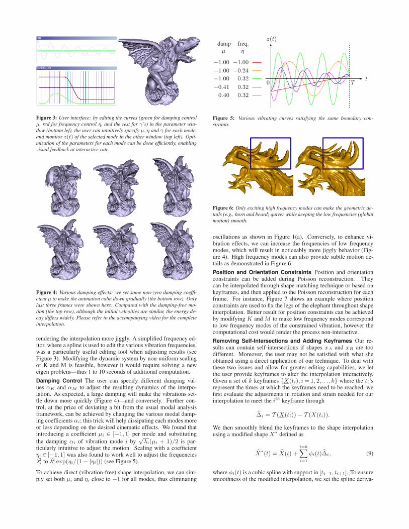
Figure 3: User interface: by editing the curves (green for damping control

µ, red for frequency control η, and the rest for γ’s) in the parameter win-

dow (bottom lef), the user can intuitively specify µ, η and γ for each mode,

and monitor z(t) of the selected mode in the other window (top left). Opti-

mization of the parameters for each mode can be done efficiently, enabling

visual feedback at interactive rate.

Figure 4: Various damping effects: we set some non-zero damping coeffi-

cient µ to make the animation calm down gradually (the bottom row). Only

last three frames were shown here. Compared with the damping-free mo-

tion (the top row), although the initial velcoities are similar, the energy de-

cay differs widely. Please refer to the accompanying video for the complete

interpolation.

rendering the interpolation more jiggly. A simplified frequency ed-itor, where a spline is used to edit the various vibration frequencies,was a particularly useful editing tool when adjusting results (seeFigure 3). Modifying the dynamic system by non-uniform scalingof K and M is feasible, however it would require solving a neweigen problem—thus 1 to 10 seconds of additional computation.

Damping Control The user can specify different damping val-ues αK and αM to adjust the resulting dynamics of the interpo-lation. As expected, a large damping will make the vibrations set-tle down more quickly (Figure 4)—and conversely. Further con-trol, at the price of deviating a bit from the usual modal analysisframework, can be achieved by changing the various modal damp-ing coefficients αi; this trick will help dissipating each modes moreor less depending on the desired cinematic effects. We found thatintroducing a coefficient µi ∈ [−1, 1] per mode and substituting

the damping αi of vibration mode i by√

λi(µi + 1)/2 is par-ticularly intuitive to adjust the motion. Scaling with a coefficientηi ∈ [−1, 1] was also found to work well to adjust the frequenciesλ2

i to λ2i exp(ηi/(1 − |ηi|)) (see Figure 5).

To achieve direct (vibration-free) shape interpolation, we can sim-ply set both µi and ηi close to −1 for all modes, thus eliminating

0t

T

z(t)damp freq.

µ η

−1.00 −1.00

−1.00 −0.24

−1.00 0.32

−0.41 0.32

0.40 0.32

Figure 5: Various vibrating curves satisfying the same boundary con-

straints.

Figure 6: Only exciting high frequency modes can make the geometric de-

tails (e.g., horn and beard) quiver while keeping the low frequencies (global

motion) smooth.

oscillations as shown in Figure 1(a). Conversely, to enhance vi-bration effects, we can increase the frequencies of low frequencymodes, which will result in noticeably more jiggly behavior (Fig-ure 4). High frequency modes can also provide subtle motion de-tails as demonstrated in Figure 6.

Position and Orientation Constraints Position and orientationconstraints can be added during Poisson reconstruction. Theycan be interpolated through shape matching technique or based onkeyframes, and then applied to the Poisson reconstruction for eachframe. For instance, Figure 7 shows an example where positionconstraints are used to fix the legs of the elephant throughout shapeinterpolation. Better result for position constraints can be achievedby modifying K and M to make low frequency modes correspondto low frequency modes of the constrained vibration, however thecomputational cost would render the process non-interactive.

Removing Self-Intersections and Adding Keyframes Our re-sults can contain self-intersections if shapes xA and xB are toodifferent. Moreover, the user may not be satisfied with what sheobtained using a direct application of our technique. To deal withthese two issues and allow for greater editing capabilities, we letthe user provide keyframes to alter the interpolation interactively.Given a set of k keyframes {X(ti), i = 1, 2,. . ., k} where the ti’srepresent the times at which the keyframes need to be reached, wefirst evaluate the adjustments in rotation and strain needed for ourinterpolation to meet the ith keyframe through

∆i = T (X(ti)) − T (X(ti)).

We then smoothly blend the keyframes to the shape interpolationusing a modified shape X∗ defined as

X∗(t) = X(t) +i=k∑

i=1

φi(t)∆i, (9)

where φi(t) is a cubic spline with support in [ti−1, ti+1]. To ensuresmoothness of the modified interpolation, we set the spline deriva-

Figure 7: The feet of the elephant will not stay firmly on the ground if we

only use barycenter position constraint in Poisson reconstruction (top row).

Position constraints (the red dots) can thus be used to control the placement

of the feet.

tives at ti−1, ti and ti+1 to 0. This simple procedure offers addi-tional control over the results as Figure 8 demonstrates. As shownin Figure 9, interpolating multiple key frames with Wiggly Splinesis also straightforward. After converting key frames into modal co-ordinates, we specify internal nodes for the vibration curve of eachmode through Wiggly Splines, which makes the interpolation curve“as physical as possible” for that mode. Note that velocity con-straints could also be incorporated. Thus, our approach provides asimple computation of nonlinear modes a la Wiggly Splines, insteadof going through linear PCA of large deformation simulations.

Quasi-Statics vs. Dynamics While our method provides an intu-itive way to design dynamic interpolation between shapes, the usermay want to start from an existing, quasi-static shape interpolationX(t) (obtained through [Sumner and Popovic 2004; Xu et al. 2005;Kilian et al. 2007], or [Adams et al. 2008] for instance) and add os-cillations to this prescribed shape interpolation. This is achieved by

computing the transform X(t) := T (X(t)) of the input shape se-

quence (we will write its coordinates as: X={log R(X)i, S(X)i}).Now the only changes in our dynamic interpolation procedure are

to substitute X(t)= (1−γ)X+ γWz(t) (γ is used to determine

Figure 8: Self-intersections (top row) can be resolved by adjusting a frame

(top, center) to be intersection free (bottom), and inserting this adjusted

shape as a key frame along the interpolation. Self-intersections in nearby

frames will then be avoided, while the vibration effects in the whole inter-

polation are kept nearly intact.

the amplitude of the vibrations) for Eq. (6) and to modify the shapereconstruction to take the given quasi-static path into account bysolving:

arg minx

‖Gx−[(exp(γ log(Ri)+(1 − γ) log R(X)i)

(Id+ γSi+(1 − γ)S(X)i)]‖2

subject to1

n

n∑

i=1

xi = c.

With these minor modifications, the main motion (given as a quasi-static motion that interpolates xA and xB) is enriched with sec-ondary deformations (based on our extended modal analysis) thatcan be controlled with intuitive parameters.

Other Vibration Modes Although we used the vibration modesresulting from modal analysis in our exposition, any other pro-cess can be used as long as a series of “characteristic” displace-ments {Wi} are produced. While the eigenmodes we use can betweaked by changing the Lame coefficients of the elastic poten-tial (or even by using spatially-varying material coefficients), wealso tried using thin-shell elastic model [Grinspun et al. 2003] asshown in Figure 10. After calculating the linear vibration modesand corresponding frequency of the triangle mesh, we evaluate thedeformation gradient by adding a fourth node for each triangle asproposed in [Sumner and Popovic 2004]. As expected, the modesvisually correspond to whatever model we selected, and the non-linear extension presented in Section 2.2.2 can be performed as isindependently of what was used to generate the basic eigenmodes.

(a) (b) (c) (d)

Figure 10: We can interpolate between triangle meshes as well, using a

deformation model governed by thin-shell elastic energy. The rest shape

is (a). The key frames in this example are (a) and (d). (b) and (c) are

intermediate frames in the animation sequence obtained by our method.

4 Implementation Details and Performance

4.1 Rotation-Strain Coordinates under Excessive Twists

When the start or end shape is extremely twisted, the log(R) ofadjacent elements computed according to Section 2.1 may have op-posite signs. During the interpolation, such elements will rotate inalmost opposite directions, leading to salient artifacts. To addressthis issue and project such poses to their correct rotation-strain co-ordinates, we traverse the elements in the mesh with a breadth-firstsearch starting from a seed tet element. When we find an elementwith its unit rotation axis differing greatly from those of its (tra-versed) neighbors (the dot product of the unit rotation axes <−0.5),we adjust the rotation angle by adding or subtracting the smallesttimes of 2π to solve this problem.

4.2 Initial value for Levenberg-Marquart Optimization

We set the initial value to ω′i = ωi, α

′i = αi for the Levenberg-

Marquart routine which is used for the optimization problem in-troduced in Section 2.3. Although the routine may be trapped inlocal minima, in most of the cases, the results turn out satisfactory.In rare cases, it fails to converge or produces very poor result (withunreasonably large initial velocity). Simply trying several (less than5 in our experience) different random initial values around ωi andαi solves this problem.

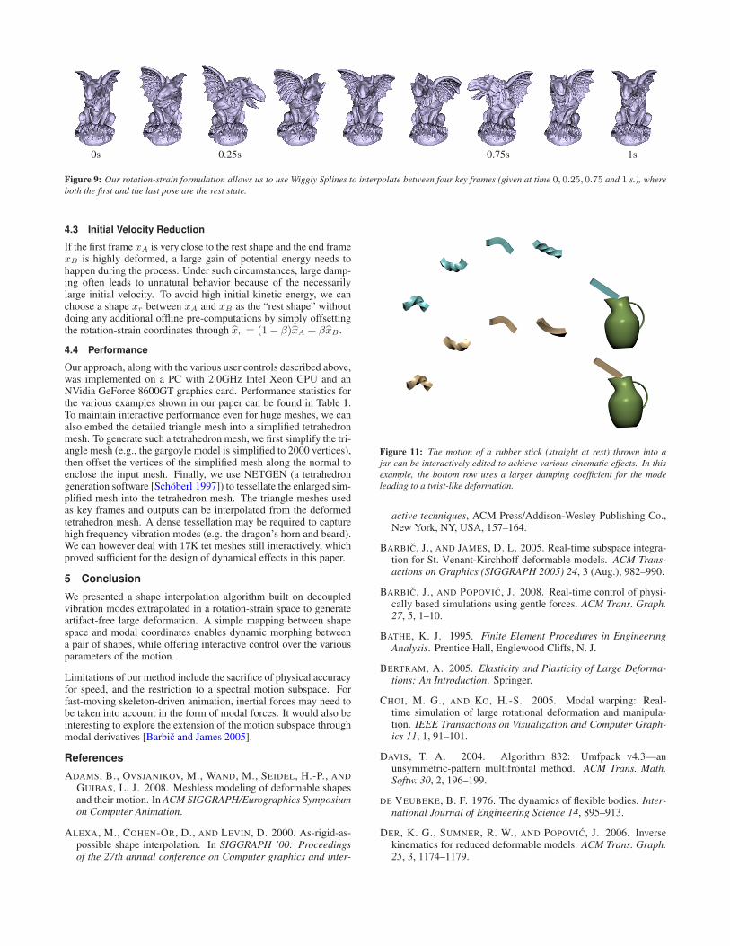
0s 0.25s 0.75s 1s

Figure 9: Our rotation-strain formulation allows us to use Wiggly Splines to interpolate between four key frames (given at time 0, 0.25, 0.75 and 1 s.), where

both the first and the last pose are the rest state.

4.3 Initial Velocity Reduction

If the first frame xA is very close to the rest shape and the end framexB is highly deformed, a large gain of potential energy needs tohappen during the process. Under such circumstances, large damp-ing often leads to unnatural behavior because of the necessarilylarge initial velocity. To avoid high initial kinetic energy, we canchoose a shape xr between xA and xB as the “rest shape” withoutdoing any additional offline pre-computations by simply offsettingthe rotation-strain coordinates through xr = (1 − β)xA + βxB .

4.4 Performance

Our approach, along with the various user controls described above,was implemented on a PC with 2.0GHz Intel Xeon CPU and anNVidia GeForce 8600GT graphics card. Performance statistics forthe various examples shown in our paper can be found in Table 1.To maintain interactive performance even for huge meshes, we canalso embed the detailed triangle mesh into a simplified tetrahedronmesh. To generate such a tetrahedron mesh, we first simplify the tri-angle mesh (e.g., the gargoyle model is simplified to 2000 vertices),then offset the vertices of the simplified mesh along the normal toenclose the input mesh. Finally, we use NETGEN (a tetrahedrongeneration software [Schoberl 1997]) to tessellate the enlarged sim-plified mesh into the tetrahedron mesh. The triangle meshes usedas key frames and outputs can be interpolated from the deformedtetrahedron mesh. A dense tessellation may be required to capturehigh frequency vibration modes (e.g. the dragon’s horn and beard).We can however deal with 17K tet meshes still interactively, whichproved sufficient for the design of dynamical effects in this paper.

5 Conclusion

We presented a shape interpolation algorithm built on decoupledvibration modes extrapolated in a rotation-strain space to generateartifact-free large deformation. A simple mapping between shapespace and modal coordinates enables dynamic morphing betweena pair of shapes, while offering interactive control over the variousparameters of the motion.

Limitations of our method include the sacrifice of physical accuracyfor speed, and the restriction to a spectral motion subspace. Forfast-moving skeleton-driven animation, inertial forces may need tobe taken into account in the form of modal forces. It would also beinteresting to explore the extension of the motion subspace throughmodal derivatives [Barbic and James 2005].

References

ADAMS, B., OVSJANIKOV, M., WAND, M., SEIDEL, H.-P., AND

GUIBAS, L. J. 2008. Meshless modeling of deformable shapesand their motion. In ACM SIGGRAPH/Eurographics Symposiumon Computer Animation.

ALEXA, M., COHEN-OR, D., AND LEVIN, D. 2000. As-rigid-as-possible shape interpolation. In SIGGRAPH ’00: Proceedingsof the 27th annual conference on Computer graphics and inter-

Figure 11: The motion of a rubber stick (straight at rest) thrown into a

jar can be interactively edited to achieve various cinematic effects. In this

example, the bottom row uses a larger damping coefficient for the mode

leading to a twist-like deformation.

active techniques, ACM Press/Addison-Wesley Publishing Co.,New York, NY, USA, 157–164.

BARBIC, J., AND JAMES, D. L. 2005. Real-time subspace integra-tion for St. Venant-Kirchhoff deformable models. ACM Trans-actions on Graphics (SIGGRAPH 2005) 24, 3 (Aug.), 982–990.

BARBIC, J., AND POPOVIC, J. 2008. Real-time control of physi-cally based simulations using gentle forces. ACM Trans. Graph.27, 5, 1–10.

BATHE, K. J. 1995. Finite Element Procedures in EngineeringAnalysis. Prentice Hall, Englewood Cliffs, N. J.

BERTRAM, A. 2005. Elasticity and Plasticity of Large Deforma-tions: An Introduction. Springer.

CHOI, M. G., AND KO, H.-S. 2005. Modal warping: Real-time simulation of large rotational deformation and manipula-tion. IEEE Transactions on Visualization and Computer Graph-ics 11, 1, 91–101.

DAVIS, T. A. 2004. Algorithm 832: Umfpack v4.3—anunsymmetric-pattern multifrontal method. ACM Trans. Math.Softw. 30, 2, 196–199.

DE VEUBEKE, B. F. 1976. The dynamics of flexible bodies. Inter-national Journal of Engineering Science 14, 895–913.

DER, K. G., SUMNER, R. W., AND POPOVIC, J. 2006. Inversekinematics for reduced deformable models. ACM Trans. Graph.25, 3, 1174–1179.

model mesh vertices tet nodes tet elements modes eigen. opt. X(t) = Wz(t) T −1(X) fps

box 440 440 1337 50 1s 6ms 2ms 8ms 70

elephant 9k 1636 5442 50 6s 6ms 6ms 33ms 20

armadillo 17k 1628 5249 100 7s 12ms 12ms 30ms 18

dragon 10k 2678 9237 100 11s 12ms 22ms 55ms 10

gargoyle 10k 2957 11054 100 12s 12ms 24ms 62ms 9

hat 1607 4771 3164 50 7s 6ms 9ms 25ms 23

Table 1: Performance statistics for the models presented in this paper; eigen. indicates the time it took to perform eigenanalysis using Matlab, while opt. gives

timings of the Levenberg-Markart optimization.

Figure 12: Synchronized armadillo diving team: adjusting frequency &

damping parameters and adding key frames lead to various flight styles

along the dive of an armadillo. The left column is the result by smooth,

vibration-free interpolation. The middle one shows moderate dynamical ef-

fects. With one intermediate keyframe (the 3rd model from the top of the

right most column), we add a tuck motion to the dive.

FENG, W.-W., KIM, B.-U., AND YU, Y. 2008. Real-time datadriven deformation using kernel canonical correlation analysis.In SIGGRAPH ’08: ACM SIGGRAPH 2008 papers, ACM, NewYork, NY, USA, 1–9.

GRINSPUN, E., HIRANI, A. N., DESBRUN, M., AND SCHRODER,P. 2003. Discrete shells. In SCA ’03: Proceedings of the 2003ACM SIGGRAPH/Eurographics symposium on Computer ani-mation, Eurographics Association, Aire-la-Ville, Switzerland,Switzerland, 62–67.

HAUSER, K., SHEN, C., AND O’BRIEN, J. F. 2003. Interactivedeformations using modal analysis with constraints. In Proceed-ings of Graphics Interface 2003, 247—256.

IGARASHI, T., MOSCOVICH, T., AND HUGHES, J. F. 2005. As-rigid-as-possible shape manipulation. ACM Trans. Graph. 24, 3,1134–1141.

JAMES, D. L., AND PAI, D. K. 2002. Dyrt: dynamic responsetextures for real time deformation simulation with graphics hard-ware. In SIGGRAPH ’02: Proceedings of the 29th annual con-

ference on Computer graphics and interactive techniques, ACM,New York, NY, USA, 582–585.

KASS, M., AND ANDERSON, J. 2008. Animating oscillatory mo-tion with overlap: wiggly splines. ACM Trans. Graph. 27, 3,1–8.

KILIAN, M., MITRA, N. J., AND POTTMANN, H. 2007. Geomet-ric modeling in shape space. ACM Trans. Graphics 26, 3. Proc.SIGGRAPH.

MULLER, M., DORSEY, J., MCMILLAN, L., JAGNOW, R., AND

CUTLER, B. 2002. Stable real-time deformations. In SCA ’02:Proceedings of the 2002 ACM SIGGRAPH/Eurographics sym-posium on Computer animation, ACM, New York, NY, USA,49–54.

NEALEN, A., MUELLER, M., KEISER, R., BOXERMAN, E., AND

CARLSON, M. 2006. Physically based deformable models incomputer graphics. Computer Graphics Forum 25, 4 (Decem-ber), 809–836.

PENTLAND, A., AND WILLIAMS, J. 1989. Good vibrations:modal dynamics for graphics and animation. In ACM SIG-GRAPH Proceedings, 215–222.

POPA, T., ZHOU, Q., BRADLEY, D., KRAEVOY, V., FU, H.,SHEFFER, A., AND HEIDRICH, W. 2009. Wrinkling capturedgarments using space-time data-driven deformation. ComputerGraphics Forum (Proc. Eurographics) 28, 2.

POPOVIC, Z., AND WITKIN, A. 1999. Physically based motiontransformation. In SIGGRAPH ’99: Proceedings of the 26thannual conference on Computer graphics and interactive tech-niques, 11–20.

POPOVIC, J., SEITZ, S. M., ERDMANN, M., POPOVIC, Z., AND

WITKIN, A. 2000. Interactive manipulation of rigid body simu-lations. In SIGGRAPH ’00: Proceedings of the 27th annual con-ference on Computer graphics and interactive techniques, 209–217.

SCHOBERL, J. 1997. Netgen - an advancing front 2d/3d-meshgenerator based on abstract rules. Comput. Visual. Sci, 1:41–52.

SUMNER, R. W., AND POPOVIC, J. 2004. Deformation transferfor triangle meshes. ACM Trans. Graph. 23, 3, 399–405.

WITKIN, A., AND KASS, M. 1988. Spacetime constraints. InSIGGRAPH ’88: Proceedings of the 15th annual conference onComputer graphics and interactive techniques, 159–168.

XU, D., ZHANG, H., WANG, Q., AND BAO, H. 2005. Poissonshape interpolation. In Proceedings of the ACM Symposium onSolid and Physical Modeling, 267–274.