Computers and Geotechnics 81 (2017) 112–124

Contents lists available at ScienceDirect

Computers and Geotechnics

journal homepage: www.elsevier .com/ locate/compgeo

Research Paper

Interaction of fluid–solid–geomembrane by the material point method

http://dx.doi.org/10.1016/j.compgeo.2016.07.0140266-352X/� 2016 Elsevier Ltd. All rights reserved.

⇑ Corresponding author.E-mail address: fursan.hamad@igs.uni-stuttgart.de (F. Hamad).URL: http://www.uni-stuttgart.de/igs (F. Hamad).

Fursan Hamad a,⇑, Zdzisław Wieckowski b, Christian Moormann a

a Institute of Geotechnical Engineering, University of Stuttgart, Pfaffenwaldring 35, 70569 Stuttgart, GermanybDepartment of Mechanics of Materials, Łódz University of Technology, Al. Politechniki 6, 90-924 Łódz, Poland

a r t i c l e i n f o

Article history:Received 4 April 2016Received in revised form 27 July 2016Accepted 28 July 2016

Keywords:Material point methodFluid–solid–geomebrane interactionGeo-container installation

a b s t r a c t

A dynamic, large deformation problem of fluid–solid–geomembrane interaction is analysed by the use ofmaterial point method, a variant of the finite element method stated in a Lagrangian–Eulerian format. Alow-order element is used for space discretisation and the fluid is treated as a compressible liquid with ahigh value of bulk modulus. Therefore, two algorithms known from literature are applied to mitigate theeffects related to the volumetric locking phenomenon. Moreover, a procedure of detecting the free sur-face is proposed. The method is applied to problems of determining the shape of geo-tubes, collapsingwater column, and finally, to the problem of installation of a geo-container on the bed of a water reser-voir. The obtained numerical outcomes are compared with the experimental results and the analytic oneswhen available.

� 2016 Elsevier Ltd. All rights reserved.

1. Introduction

Geosynthetic materials have a growing use in geomechanicalapplications as a construction material. In coastal and hydraulicengineering, the innovative use of thin geosynthetics combinedwith dredged materials provides efficient alternative for conven-tional materials. Applications of geotextiles and geosynthetics incoastal engineering are addressed in more detail by Pilarczyk[37]. One of the major concerns of manufacturers and engineersis to build units that are able to sustain the installation process,though it is commonly associated with large material deformation.Geotextile containers can experience high stresses. The risks ofgeocontainers bursting in deep water, inaccurate placement dueto waves and currents, or even the slope failure of a heap of geo-containers are important issues that influence the feasibility ofusing geocontainers [14]. Several field and lab tests have been per-formed to study the placement history of the containers whichincluded measuring the fall velocity and strains in the geotextile[6,5]. The numerical modelling of the thin-walled structures joinedwith history-dependent material subjected to large deformation inthe presence of water is a challenging topic for the traditionalmethods. Simulation of the entire process contributes to theunderstanding of the flow field around the container, particularlywhen a geocontainer hits the ground.

In order to avoid problems associated with mesh distortionsand element entanglements in the finite element method formu-lated in a Lagrangian framework, large deformation problems canbe solved using point-based (meshfree) methods. These methodstrace the history of state variables at points that are independentof the mesh. In some of these methods, no mesh is used and thefield approximation is built on the basis of a set of points only.Examples of these methods are: methods using the movingweighted least-square approximation (MWLS) such as the gener-alised finite difference method [30], the diffuse element methodand the element-free Galerkin method [3]; kernel methods suchas the smoothed particle hydrodynamics method (SPH) [31] andthe reproducing kernel particle method (RKPM); partition of unitymethods [35]; the radial basis functions method [44] and the mov-ing kriging interpolation method [13]. A survey of the point-basedmethods can be found, for example, in Ref. [28]. Discrete elementmethod (DEM) is applied widely to simulate the interaction ofgranular materials with structures [23,16,42]. One of the point-based methods is the particle–in–cell method (PIC), which hasbeen used in fluid dynamics since 1964 [21]. The PIC methodwas adapted by Sulsky et al. [40] to solid mechanics problems.The adaptation was called the material point method (MPM).MPM represents the continuum by a collection of material points,whereas field information is transferred from these points to thebackground computational grid which can be arbitrarily definedor constant, particularly. As the background mesh (of an Euleriantype) is freely chosen, the problem of severe mesh distortion isavoided. Because the arbitrary Lagrangian–Eulerian description ofmotion utilised in the method, MPM is well-suited for large

F. Hamad et al. / Computers and Geotechnics 81 (2017) 112–124 113

deformation problems of fluid and solid mechanics. The unifiedcomputational framework in MPM allows including various mate-rials as well as structural elements. The method has been success-fully applied to granular flow [45,46] and geotechnical [45,4]problems, simulation of motion of a geo–container dropped froma split barge [17,19] and other problems [25,11]. The process ofdropping of a geocontainer in water has been modelled by theuse of two-dimensional MPM implementation in [47].

When linear interpolation functions are used in MPM version,mapping the velocity field from the computational mesh to thematerial points is straightforward. This type of shape functions isbecoming more popular in modelling incompressible fluid as itmakes it free from non-physical (spurious) deformation modesthat are associated with high-order elements [49]. However, thehigh value of bulk modulus of liquids causes numerical instabilitywhich requires applying a stabilisation technique. The instabilityassociated with the explicit modelling of near incompressible fluidhas been improved by introducing some enhancement techniques.As the spherical component of the stress is blamed for numericaldifficulties, different techniques based on mixed formulation areutilised to circumvent the volumetric locking problem when low-order elements are used. Zienkiewicz and Taylor [49] summarisethese methods and describe the corresponding mathematical back-ground. To mitigate locking and spurious pressure variations,numerical schemes based on splitting the differential operatorare popular. The fractional step method (FSM) or characteristic-based-split procedure (CBS) is widely used to obtain the solutionfor an incompressible fluid problem [36]. An extensive studyrelated to these methods is provided in [49] and the referencestherein. Detournay and Dzik [15] discuss some methods valid forhistory–dependent materials. Their approach was then examinedin MPM by Stolle et al. [38]. Extension of this work to a two-phase material subjected to small deformation is implemented in[26,1], where the enhancement approach is applied for soil andwater separately. For large deformation problems, the work byMast et al. [34] is based on averaging spherical component insidethe cell as well as inside elements located around the computa-tional grid node to mitigate locking.

In the present work, a combination of nodal mixed discretisa-tion (NMD) and average nodal pressure (ANP) approaches areapplied to alleviate the locking phenomenon associated with theuse of the low-order element in MPM for nearly incompressiblefluid. The enhanced algorithm has been tested for a practical appli-cation of the geotube for which the analytic solution is available inthe case of a simplified model. The aim of the comparison is tocheck if the MPM solution converges to the steady state analyticsolution and to evaluate the interaction of the fluid with the geo-textile elements. In order to examine the capacity of the suggestedmethod to capture the real dynamic process, the problem of watercolumn collapse has been reproduced. Furthermore, the free sur-face condition of the flowing fluid is detected by evaluating thecontinuous mass density field on the basis of the discrete massesof the material points. As an application of the soil–water–geotextile interaction, the experiment of dropping small soil containerinto water tank performed at GeoDelft/Deltares by Bezuijen et al.[5] is modelled.

This paper is organised as follows. The general algorithm ofMPM for solid and fluid materials is shown in Section 2. Then thetwo algorithms allowing to mitigate the volumetric locking aregiven in Section 3. The combination of these algorithms is thenapplied in the analysis of the geo-tube problem for which threevalues of the filling ratio are considered and the obtained resultsare compared with the analytic solution. The procedure for detect-ing the free surface in MPM and the solution to the problem ofwater column collapse are presented in Section 4. In Section 5,the results of simulation of the installation process for a

geo-container are presented. The concluding remarks are sum-marised in Section 6.

2. General algorithm of MPM

The main variables for the class of problems addressed in thispaper appear in the momentum balance equation

. €u ¼ LTrþ .g; ð1Þwhere the superposed double dot of the displacement vector u isthe time derivative, L is a linear differential operator describingthe strain–displacement relation, r is the Cauchy stress tensor rep-resented in vector form, . is the mass density, and g the gravita-tional acceleration vector. The variables are functions of position xand time t. Since the material point method is based on the Lagran-gian formulation of the equations of motion, the advection terms donot appear on the left-hand-sides of these equations. Within thecontext of MPM, the weak formulation of Eq. (1) based on virtualwork is adopted. By applying the principle of virtual work and per-forming a finite element discretisation, Eq. (1) yields

Mc a ¼ Fext � F int; ð2Þwhere Mc is the consistent mass matrix, a denotes the nodal accel-

eration vector, and Fext and F int are the external and internal nodalforce vectors, respectively (cf. [26,46]). In practice, the lumped massmatrix is preferred over the consistent one as it simplifies the com-putations due to it being diagonal, albeit at the expense of introduc-ing a slight amount of numerical dissipation [10]. In this paper, wefollow the standard MPM formulation [40,41] in which a body isdefined in terms of material points as shown in Fig. 1. In otherwords, the material properties and state variables such as the stressand momentum are defined and traced at the material points.Hence, the internal force vector in Eq. (2) is obtained as a sum overthe total number of material points np such that

F int ¼Xnpp¼1

wpBTðxpÞrp; ð3Þ

withwp being the particle volume and B ¼ LN, where N is the shapefunction matrix, and rp is a vector containing the stress compo-nents at the pth material point. The external nodal force vector isgiven by

Fext ¼Xnpp¼1

mp NTðxpÞ g þZCt

NT t dC; ð4Þ

wheremp denotes the mass corresponding to the pth material point,and t represents the prescribed traction on boundary Ct .

A forward Euler algorithm is commonly used in MPM codes tointegrate Eq. (2) in time. To improve the solution quality or toincrease the time step size, implicit integration has been intro-duced, see for example [43]. Owing to the fact that such a proce-dure constructs a stiffness matrix, the algorithm becomescomputationally expensive especially for problems with high num-ber of degrees of freedom. Moreover, it is much easier to solve thecontact problem using the explicit algorithm comparing to animplicit approach. Therefore, explicit time integration scheme isimplemented in this paper. The momentum equations are solvedon the background computational mesh which provides a conve-nient means for calculating the gradient of the velocity field. Incontrast to FEM, where integration points are tightly connectedwith mesh elements, in MPM, the material points are allowed tomove from one element to another. The state variables are tracedat the material points ‘‘flowing” through the mesh. As shown inFig. 1, the MPM calculation cycle goes through three phases: an ini-tialisation phase, where the velocity field is mapped from the

Fig. 1. Solution procedure of an MPM computational step.

114 F. Hamad et al. / Computers and Geotechnics 81 (2017) 112–124

material points to the computational grid nodes; a Lagrangianphase that parallels a finite element calculation, where the systemequations are setup and primary variables (velocity and displace-ment) are evaluated at the nodes with the stresses and strainsdetermined at the material points; and a convection phase, wherethe location of the material points is updated [46,26,11]. The pro-cedure of mapping the velocity from material points to the nodesof the computational mesh is based on the least square methodas proposed by Sulsky et al. [41].

2.1. Constitutive equations

As the interaction between a solid (granular) material, a thingeo-textile membrane and a fluid is modelled in the paper, threetypes of constitutive relations are considered. They are describedin the following subsections.

2.1.1. Solid materialFinite deformation problems are considered in the present

paper which means that one should satisfy the requirement ofobjectivity of the constitutive relations (cf. [32]). As the partialtime derivative of the stress tensor does not preserve this require-ment, the rate form of a constitutive equation should have the fol-lowing form:

r0ij

�¼ Dijkl _ekl; ð5Þ

where r0�is an objective rate of the effective stress tensor r0, _e is the

symmetric part of the velocity gradient, and D is the fourth-orderconstitutive tensor. Different forms of the objective stress rate aredefined in continuum mechanics [32,2]. Hill’s rate [22], or the co–

rotational rate of Kirchhoff stress tensor, r0ij

r, has been used in this

paper. This objective stress rate includes the effect of volumechange and has the form

r0ij

r¼ _r0

ij �xikr0kj þ r0

ikxkj þ _ekkr0ij; ð6Þ

with x being the anti–symmetric part of the velocity gradient (spintensor), and _ekk is the spherical part of the strain rate tensor.

An elastic–plastic constitutive model is utilised in this paper todescribe the mechanical behaviour of the solid material (a soil).The plastic yield function is defined by the Mohr–Coulombcondition

f ðr0Þ ¼ jr0i � r0

jj � r0i þ r0

j

� �sin/� 2c cos/ ¼ 0; ð7Þ

where r0i and r0

j; i; j ¼ 1;2;3 and i– j, are the principal stresses, c isthe cohesion, and / the friction angle. A non-associated flow rule isconsidered so that the plastic potential g has the form

g ¼ jr0i � r0

jj � r0i þ r0

j

� �sinw; ð8Þ

where w denotes the dilatancy angle. For applications where highlocal shear stresses might take place, a degradation of the strengthparameters is important to accommodate, see for example [43]. Inthis paper, the relative simple material model is utilised and post-failure effects in the soil are not taken into account.

2.1.2. Thin membraneAmembrane is a thin-walled structure that has tension stiffness

in-plane with no stiffness in bending. To describe the behaviour ofa membrane, a locally-rotated frame of reference is defined so thatthe plane stress condition can be easily applied. A linear elasticmembrane is considered in this paper, however, nonlinearity asso-ciated with finite deformation is included. In addition, the beha-viour of geo-textile materials implies sustaining the tensile forcesbut not compressive ones. Hence, the constitutive model of themembrane should include a proper criteria to cut the compressionstresses off which is introduced as a compression cut–off criterion.In this formulation, folds and wrinkles of the membrane are notconsidered but rather a simplified approach is implemented byadjusting the principal stresses to be non-negative. A similar tech-nique is adopted for geomechanical applications in the commercialsoftware Plaxis [9]. Using the definition of the co-rotational stresstensor r, the principal stresses are given as

rI; II ¼ r11 þ r22

2� rm; ð9Þ

where rI and rII are the major and minor principal in–plane mem-brane stresses in the local coordinates, and

rm �ffiffiffiffiffiffiffiffiffiffiffiffiffiffiffiffiffiffiffiffiffiffiffiffiffiffiffiffiffiffiffiffiffiffiffiffiffiffiffiffiffiffiffiffiffiffiffiffiffiffiffiffiffiffiððr11 � r22Þ=2Þ2 þ ðr12Þ2

qis the radius of the Mohr circle. The

compression cut-off criterion requires thatboth theprincipal stressesare non-negative, otherwise, a stress correction should be applied.

When an elastic stress predictor, r11; r22, r12, calculated duringcomputations gives a negative value for the minor principal co-rotational stress,

rII < 0;

the stress correction is done by means of homothetic transforma-tion of Mohr’s stress circle (see Fig. 2). The Mohr circle related tothe predicted stresses–drawn with a dashed line–is transformedto the circle–drawn with a solid line–with homothety centre S.The homothety ratio of the transformation can be read from thefigure,

k ¼ rI

rI � rII� rI

2 rm:

The corrected values of the co-rotational stress components can bederived from the following equations:

rI � rcorr11 ¼ kðrI � r11Þ;

rcorr11 þ rcorr

22 ¼ rI;

rcorr12 ¼ kr12:

Fig. 2. Stress correction interpretation.

F. Hamad et al. / Computers and Geotechnics 81 (2017) 112–124 115

The solution of the above equations has the form

rcorr11 ¼ rI 1� rI � r11

2rm

� �;

rcorr22 ¼ rI 1� rI � r22

2rm

� �;

rcorr12 ¼ rI

r12

2rm:

ð10Þ

The membrane element is combined in MPM by modifying thegeneral algorithm to consider the in-plane membrane effect of asingle layer of material points [48]. Alternatively, the membranecan be treated as a finite element structure inside the MPM frame.Hamad et al. [17] provide a detailed formulation and comparison ofthe two approaches as well as the interaction with solid materials,which shows that the coupled approach predicts stresses moreaccurately with coarser discretisation. More applications aboutthe coupling procedure can be found in [18]. In this paper, theFEM–MPM coupled algorithm is followed for the membraneformulation.

2.1.3. Compressible fluidWater behaviour is described in the paper using the model of

isotropic viscous fluid the constitutive relation for which can bewritten in the following form (cf. [32,49]):

rij ¼ �pdij þ k _ekk dij þ 2l _eij; ð11Þwhere p is the pressure, dij the Kronecker delta, whereas k and l areindependent parameters characterising the viscosity of the fluid.After introducing the rate-of-deformation tensor in terms of thedeviatoric and spherical components, _eij ¼ _e0ij þ _ekk dij=3 with _e0ijbeing the deviatoric strain rate, Eq. (11) can be formulated asfollows

rij ¼ �pþ j _ekkð Þdij þ 2l _e0ij; ð12Þ

where j ¼ kþ 23 l denotes the volumetric viscosity. Neglecting

(after Stokes) the term related to volumetric viscosity, j _ekk (with-out setting _ekk ¼ 0), the constitutive relation for viscous fluid maytake the form

rij ¼ �pdij þ 2l _e0ij: ð13ÞAs the use of an explicit algorithm for solving the equations ofmotion is intended in the present paper, the compressible fluid is

considered in the analysis. The density change, as a result of elasticdeformation, is related to the pressure change via equation

@.@t

¼ 1c2p

@p@t

; ð14Þ

where cp ¼ffiffiffiffiffiffiffiffiffiffiffiKf =.

pis the acoustic wave speed with Kf being the

elastic bulk modulus of the fluid. For a compressible fluid subjectedto an isothermal process, the pressure–density relation might takethe form [29]

ppref

¼ ..ref

� �j

� 1; ð15Þ

where the subscript �ð Þref indicates a reference value and j is amaterial parameter. More sophisticated relationships can be estab-lished, although they need more parameters to calibrate. Eq. (15)can be replaced by a linear formula for a relatively wide range ofpressure so that

p ¼ pref � Kf ev ; ð16Þwith ev being the volumetric strain and pref the reference pressure.

2.2. MPM solution procedure

Although the interaction of three different bodies, soil, fluid anda thin membrane, is analysed in the present paper, the appliedsolution procedure does not differ essentially from the MPM algo-rithm proposed in [40,41]. It is assumed that subregions of theanalysed bodies (not overlapping themselves) are represented bymaterial points so that the field of mass density can be expressedas follows:

.ðxÞ ¼Xp

mp dðx� xpÞ; ð17Þ

where mp and xp denote the mass and position of the pth materialpoint, respectively, while d is the Dirac delta distribution. The dis-crete equations of motion (2) are solved in an incremental way byuse of an explicit integration algorithm for each time increment.For the nth time increment, the acceleration nodal vector, an, is cal-culated from the equation

an ¼ Mnð Þ�1 Fext;n � F int;n� �

; ð18Þ

with Mn being the diagonalized mass matrix, Fext and F int are givenin Equations (4) and (3), respectively. The velocities of the materialpoints are calculated using the interpolation functions related to thecomputational mesh and nodal accelerations,

vnþ1p ¼ vn

p þXi

DtNi;p ani ; ð19Þ

where Dt is the time increment, the summation index i varies from1 to the number of nodes per element and Ni;p is the value of theshape function for node i evaluated at the location of the pth mate-rial point.

Subsequently, the stress field in the fluid is evaluated usingEquations (13) and (16). The appropriate constitutive models forthe material points representing soil and the membrane describedin Sections 2.1.1 and 2.1.2, respectively, are then applied to get the

updated stress field ðr0Þnþ1. The strain increment needed for theintegration of the constitutive relations is calculated on the basisof the nodal velocities and the gradient of the interpolationfunctions.

Next, the velocities of the material points are projected onto thecomputational mesh; the nodal velocities are calculated by solvingthe following linear system of equations [40]

116 F. Hamad et al. / Computers and Geotechnics 81 (2017) 112–124

Mnvnþ1 ¼Xnpp¼1

mpNTp v

nþ1p ; ð20Þ

where np is the total number of material points. The MPM mappingprocedure avoids the non-physical disconnections of points locatedon the surface of the analysed body. This phenomenon mightappear when an element exists inside which a single material pointis located closely to a face of an element (in the three-dimensionalcase) or edge (in the two-dimensional case). In the case of elementswith linear shape functions, the mass matrix term related to thenode opposite to this face or edge is very small but the gradientsof the shape functions are independent of the point position, anda large value of acceleration at this node is obtained as an effect.The similar situation appears also if another material point islocated in the same element close to the same face or edge. Eq.(20), as a result of the least square method used in the projectionprocedure, provides a smooth velocity field eliminating disconnec-tions of surface points from the rest of the body.

The position of the material points is updated using the nodalvalues of the velocity field and the interpolation functions fromthe following expression:

xnþ1p ¼ xnp þ

Xi

DtNi;p vnþ1i : ð21Þ

3. Volumetric locking: existence and alleviation

In the displacement finite element method, when linear shapefunctions are utilised, a volumetric locking is expected to appeardue to a poor representation of an isochoric displacement field.Therefore, the material tends to show non-physical stiffnessagainst deformation when it has a high bulk modulus. Numerousmethods were presented in the FE framework (cf. [49]). Inboundary-value problems, the kinematic locking due to the highbulk modulus spreads through the entire body domain and leadsto underpredicted values of the velocities, with oscillations inthe pressure field known as a checkerboard pressure pattern. Asthe locking problem is associated with the spherical componentof the stress tensor, a mixed formulation provides a suitablescheme, where more than one unknown field variables are defined[2,49]. Therefore, the pressure or the volumetric strain can bedefined as an independent degree of freedom on the discretisationgrid beside velocities. The fractional step method (FSM) or anyother scheme based on splitting the governing differential equa-tions can be introduced [36]. In this paper, two enhancementschemes based on a single discretisation are examined. The back-ground of the two approaches with the mathematical derivation isprovided by Detournay and Dzik [15] for elastic and elasto–plasticmaterials.

3.1. Nodal mixed discrestisation (NMD)

The nodal mixed discretisation technique keeps the deviatoricstrain part as it is done in the standard discretisation and makesuse of averaging the volumetric strain over elements contactingat a common vertex. As a result, the smoothed volumetric part ofthe strain tensor alleviates the locking problem. The smoothed vol-umetric strain rate is expressed with the use of shape functions Nas follows:�_ev ¼ N �_ev ; ð22Þwhere �_ev is the vector of nodal values that are found by solving theminimisation problem (least square method) in the formZXðN �_ev � _evÞ2 dX ¼ min

in which the volumetric strain rate, _ev , is compatible with the veloc-ity field, v , such that

_ev ¼ Bv v � @N1@x

@N1@y

@N2@x

@N2@y � � �

h iv:

The solution of the above problem, �_ev , satisfies the following systemof linear algebraic equations:ZXNTN dX�_ev ¼

ZXNT _ev dX: ð23Þ

In the case of linear shape functions, after diagonalisation of thematrix of system (23), the equation related to a specific node (num-ber i) takes the form:P

eXe

d�_ev;i ¼

PeXe _ev;ed

; ð24Þ

where the sums relate to the elements attached to the ith node, Xe

denotes the volume of the eth attached element, and d ¼ 4 whentetrahedral element is applied (or d ¼ 3 in the case of triangular ele-ments). It follows from Eq. (24) that

�_ev;i ¼P

eXe _ev;ePeXe

:

Finally, the strain rate tensor is modified in the following form:

�_e ¼ _e� 13_evdþ 1

3�_evd; ð25Þ

where d is the identity matrix and

�_ev ¼ 1d

Xd

i¼1

�_ev;i

is the averaged volumetric strain rate calculated for the centralpoint of an element using Eq. (22).

3.2. Average nodal pressure (ANP)

The average nodal pressure scheme has been proposed to alle-viate the volumetric locking for linear elements in [7,24]. In thisapproach, the pressure is evaluated at the nodes by defining nodalvolumes based on surrounding triangles or tetrahedrals. The for-mulation of the ANP scheme starts with estimating the averagevolumetric ratio Ji at the node i as follows

Ji ¼Xi

Xi;0with Xi ¼ 1

nen

Xe

Xe; ð26Þ

where the subscript 0 refers to the initial configuration and thesummation runs over the number of elements attached to the nodei. As follows, the average nodal pressure pi is computed and mappedback finally to the element, i.e.

�pe ¼ 1nen

Xneni¼1

pi with pi ¼ Kf Ji � 1ð Þ; ð27Þ

where �pe is the average element pressure. In this procedure, thespherical part of the stress tensor is evaluated at the nodes whilethe deviatoric part is kept on the element level with no change. Inthe present MPM formulation, the entire stress tensor is evaluatedat the pth material point followed by explicit averaging of thespherical component at the nodes as

r ¼ s� d�pp; ð28Þin which, the enhanced pressure �pp at the pth material point is com-puted using the formulae

�pp ¼ 1nen

Xneni¼1

�pi with �pi ¼P

eppwpPewp

; ð29Þ

F. Hamad et al. / Computers and Geotechnics 81 (2017) 112–124 117

where the summation over index e runs over the number of ele-ments attached to the node i, and wp is the volume of the subregionrepresented by the pth material point that is located in the eth ele-ment. However, in the case of MPM when particles might changeelements, the ANP approach alone is not sufficient to stabilise thepressure field and alleviate the pathological locking. Therefore,adopting both ANP and NMD approaches collectively reduces thepressure instability mitigating the volumetric locking problem.Recently, the combination of the two schemes has been appliedfor creep flow problems by Stolle et al. [39].

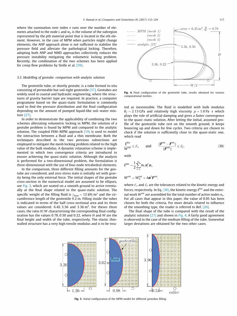
Fig. 4. Final configuration of the geotextile tube, results obtained for variouscomputational meshes.

3.3. Modelling of geotube: comparison with analytic solution

The geotextile tube, or shortly geotube, is a tube formed in-situconsisting of permeable but soil-tight geotextile [37]. Geotubes arewidely used in coastal and hydraulic engineering, where the struc-tures of gravity barrier type are required. In practice, a computerprogramme based on the quasi-static formulation is commonlyused to find the pressure distribution and the final configurationdepending on the amount of pumped liquid-like soil–water mix-ture [27].

In order to demonstrate the applicability of combining the twoschemes alleviating volumetric locking in MPM, the solution of ageotube problem is found by MPM and compared to the analyticsolution. The coupled FEM–MPM approach [19] is used to modelthe interaction between a fluid and a thin membrane. Both thetechniques described in the two previous subsections areemployed to mitigate the mesh locking problem related to the highvalue of the bulk modulus. A dynamic relaxation scheme is imple-mented in which two convergence criteria are introduced toensure achieving the quasi-static solution. Although the analysisis performed for a two-dimensional problem, the formulation isthree-dimensional with the use of four-node tetrahedral elements.

In the comparison, three different filling amounts for the geo-tube are considered, and zero stress state is initially set with grav-ity being the only external force. The initial shapes of the geotubecross-section in the numerical model are assumed to be ellipses,see Fig. 3, which are seated on a smooth ground to arrive eventu-ally at the final shape related to the quasi-static solution. Thespecific weight of the filling fluid is cfluid ¼ 12 kN=m3 and the cir-cumference length of the geotextile 9:2 m. Filling inside the tubesis indicated in terms of the half cross-sectional area and its threevalues are considered: 6:45;5:56 and 3:36 m2. For theses threecases, the ratio H=W characterising the corresponding final config-uration has the values 0:78;0:50 and 0:22, where H and W are thefinal height and width of the tube, respectively. The elastic thin-walled structure has a very high tensile modulus and is to be trea-

Fig. 3. Initial configuration of the MPM

ted as inextensible. The fluid is modelled with bulk modulusKf ¼ 2:13 GPa and relatively high viscosity l ¼ 1:0 Pa � s whichplays the role of artificial damping and gives a faster convergenceto the quasi–static solution. After letting the initial, assumed pro-file of the geotextile tube rest on the smooth ground, it keepsbouncing up and down for few cycles. Two criteria are chosen tocheck if the solution is sufficiently close to the quasi-static one,which read

Ekin

Wext 6 Ev andkFext � F intk

kFextk 6 Ef ; ð30Þ

with

Ekin ¼ 12

Xnni¼1

mivTi v i;

Wext ¼ Wext0 þ DuTFext;

where Ev and Ef are the tolerances related to the kinetic energy and

forces, respectively. In Eq. (30), the kinetic energy Ekin and the exter-nal workWext are assembled for the total number of active nodes nn.For all cases that appear in this paper, the value of 0:05 has beenchosen for both the criteria. For more details related to influenceof the smoothing type, the reader is referred to Ref. [20].

The final shape of the tube is compared with the result of theanalytic solution [27] and shown in Fig. 4. A fairly good agreementis observed in the case of the medium filling of the tube. Somewhatlarger deviations are obtained for the two other cases.

model for different geotubes filling.

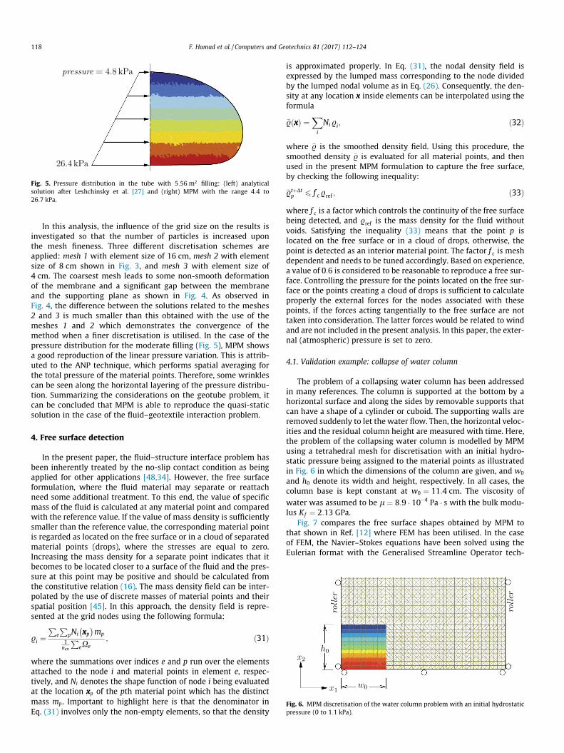
Fig. 5. Pressure distribution in the tube with 5:56 m2 filling: (left) analyticalsolution after Leshchinsky et al. [27] and (right) MPM with the range 4:4 to26:7 kPa.

Fig. 6. MPM discretisation of the water column problem with an initial hydrostaticpressure (0 to 1:1 kPa).

118 F. Hamad et al. / Computers and Geotechnics 81 (2017) 112–124

In this analysis, the influence of the grid size on the results isinvestigated so that the number of particles is increased uponthe mesh fineness. Three different discretisation schemes areapplied: mesh 1 with element size of 16 cm, mesh 2 with elementsize of 8 cm shown in Fig. 3, and mesh 3 with element size of4 cm. The coarsest mesh leads to some non-smooth deformationof the membrane and a significant gap between the membraneand the supporting plane as shown in Fig. 4. As observed inFig. 4, the difference between the solutions related to the meshes2 and 3 is much smaller than this obtained with the use of themeshes 1 and 2 which demonstrates the convergence of themethod when a finer discretisation is utilised. In the case of thepressure distribution for the moderate filling (Fig. 5), MPM showsa good reproduction of the linear pressure variation. This is attrib-uted to the ANP technique, which performs spatial averaging forthe total pressure of the material points. Therefore, some wrinklescan be seen along the horizontal layering of the pressure distribu-tion. Summarizing the considerations on the geotube problem, itcan be concluded that MPM is able to reproduce the quasi-staticsolution in the case of the fluid–geotextile interaction problem.

4. Free surface detection

In the present paper, the fluid–structure interface problem hasbeen inherently treated by the no-slip contact condition as beingapplied for other applications [48,34]. However, the free surfaceformulation, where the fluid material may separate or reattachneed some additional treatment. To this end, the value of specificmass of the fluid is calculated at any material point and comparedwith the reference value. If the value of mass density is sufficientlysmaller than the reference value, the corresponding material pointis regarded as located on the free surface or in a cloud of separatedmaterial points (drops), where the stresses are equal to zero.Increasing the mass density for a separate point indicates that itbecomes to be located closer to a surface of the fluid and the pres-sure at this point may be positive and should be calculated fromthe constitutive relation (16). The mass density field can be inter-polated by the use of discrete masses of material points and theirspatial position [45]. In this approach, the density field is repre-sented at the grid nodes using the following formula:

.i ¼P

e

PpNi xp

� �mp

1nen

PeXe

; ð31Þ

where the summations over indices e and p run over the elementsattached to the node i and material points in element e, respec-tively, and Ni denotes the shape function of node i being evaluatedat the location xp of the pth material point which has the distinctmass mp. Important to highlight here is that the denominator inEq. (31) involves only the non-empty elements, so that the density

is approximated properly. In Eq. (31), the nodal density field isexpressed by the lumped mass corresponding to the node dividedby the lumped nodal volume as in Eq. (26). Consequently, the den-sity at any location x inside elements can be interpolated using theformula

�. xð Þ ¼Xi

Ni.i; ð32Þ

where �. is the smoothed density field. Using this procedure, thesmoothed density �. is evaluated for all material points, and thenused in the present MPM formulation to capture the free surface,by checking the following inequality:

�.tþDtp 6 f c.ref ; ð33Þ

where f c is a factor which controls the continuity of the free surfacebeing detected, and .ref is the mass density for the fluid withoutvoids. Satisfying the inequality (33) means that the point p islocated on the free surface or in a cloud of drops, otherwise, thepoint is detected as an interior material point. The factor f c is meshdependent and needs to be tuned accordingly. Based on experience,a value of 0:6 is considered to be reasonable to reproduce a free sur-face. Controlling the pressure for the points located on the free sur-face or the points creating a cloud of drops is sufficient to calculateproperly the external forces for the nodes associated with thesepoints, if the forces acting tangentially to the free surface are nottaken into consideration. The latter forces would be related to windand are not included in the present analysis. In this paper, the exter-nal (atmospheric) pressure is set to zero.

4.1. Validation example: collapse of water column

The problem of a collapsing water column has been addressedin many references. The column is supported at the bottom by ahorizontal surface and along the sides by removable supports thatcan have a shape of a cylinder or cuboid. The supporting walls areremoved suddenly to let the water flow. Then, the horizontal veloc-ities and the residual column height are measured with time. Here,the problem of the collapsing water column is modelled by MPMusing a tetrahedral mesh for discretisation with an initial hydro-static pressure being assigned to the material points as illustratedin Fig. 6 in which the dimensions of the column are given, and w0

and h0 denote its width and height, respectively. In all cases, thecolumn base is kept constant at w0 ¼ 11:4 cm. The viscosity ofwater was assumed to be l ¼ 8:9 � 10�4 Pa � s with the bulk modu-lus Kf ¼ 2:13 GPa.

Fig. 7 compares the free surface shapes obtained by MPM tothat shown in Ref. [12] where FEM has been utilised. In the caseof FEM, the Navier–Stokes equations have been solved using theEulerian format with the Generalised Streamline Operator tech-

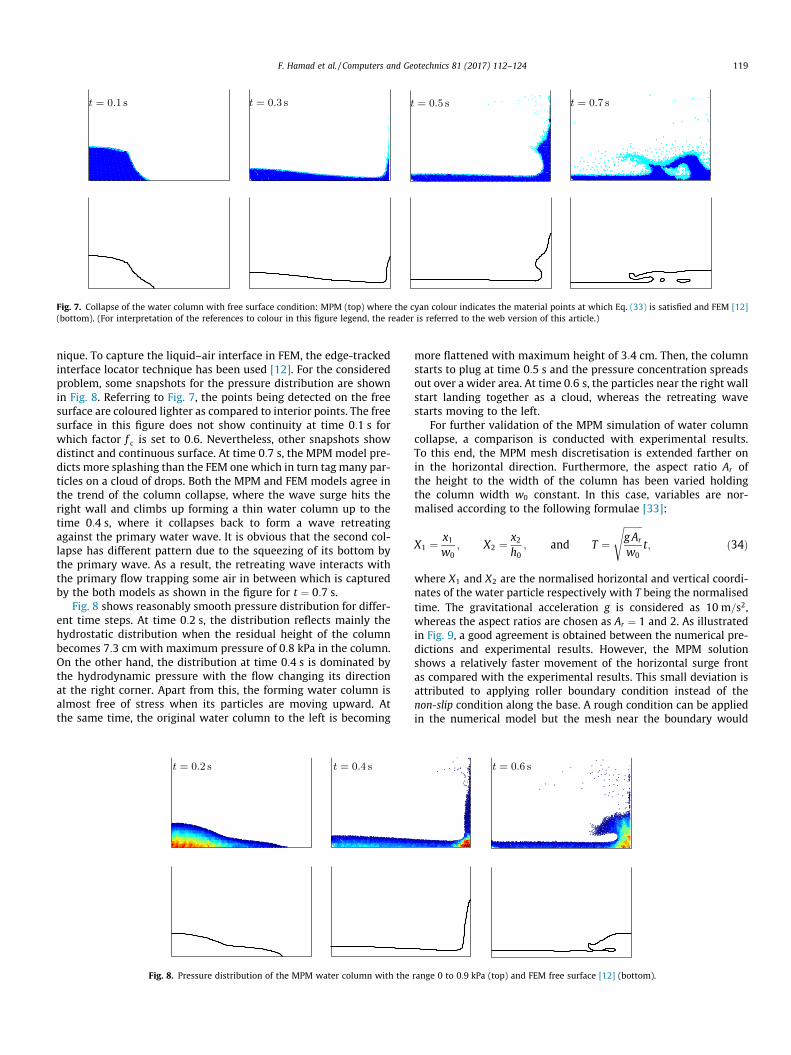
Fig. 7. Collapse of the water column with free surface condition: MPM (top) where the cyan colour indicates the material points at which Eq. (33) is satisfied and FEM [12](bottom). (For interpretation of the references to colour in this figure legend, the reader is referred to the web version of this article.)

F. Hamad et al. / Computers and Geotechnics 81 (2017) 112–124 119

nique. To capture the liquid–air interface in FEM, the edge-trackedinterface locator technique has been used [12]. For the consideredproblem, some snapshots for the pressure distribution are shownin Fig. 8. Referring to Fig. 7, the points being detected on the freesurface are coloured lighter as compared to interior points. The freesurface in this figure does not show continuity at time 0:1 s forwhich factor f c is set to 0:6. Nevertheless, other snapshots showdistinct and continuous surface. At time 0:7 s, the MPM model pre-dicts more splashing than the FEM one which in turn tag many par-ticles on a cloud of drops. Both the MPM and FEM models agree inthe trend of the column collapse, where the wave surge hits theright wall and climbs up forming a thin water column up to thetime 0:4 s, where it collapses back to form a wave retreatingagainst the primary water wave. It is obvious that the second col-lapse has different pattern due to the squeezing of its bottom bythe primary wave. As a result, the retreating wave interacts withthe primary flow trapping some air in between which is capturedby the both models as shown in the figure for t ¼ 0:7 s.

Fig. 8 shows reasonably smooth pressure distribution for differ-ent time steps. At time 0:2 s, the distribution reflects mainly thehydrostatic distribution when the residual height of the columnbecomes 7:3 cm with maximum pressure of 0:8 kPa in the column.On the other hand, the distribution at time 0:4 s is dominated bythe hydrodynamic pressure with the flow changing its directionat the right corner. Apart from this, the forming water column isalmost free of stress when its particles are moving upward. Atthe same time, the original water column to the left is becoming

Fig. 8. Pressure distribution of the MPM water column with the

more flattened with maximum height of 3:4 cm. Then, the columnstarts to plug at time 0:5 s and the pressure concentration spreadsout over a wider area. At time 0:6 s, the particles near the right wallstart landing together as a cloud, whereas the retreating wavestarts moving to the left.

For further validation of the MPM simulation of water columncollapse, a comparison is conducted with experimental results.To this end, the MPM mesh discretisation is extended farther onin the horizontal direction. Furthermore, the aspect ratio Ar ofthe height to the width of the column has been varied holdingthe column width w0 constant. In this case, variables are nor-malised according to the following formulae [33]:

X1 ¼ x1w0

; X2 ¼ x2h0

; and T ¼ffiffiffiffiffiffiffiffigAr

w0

st; ð34Þ

where X1 and X2 are the normalised horizontal and vertical coordi-nates of the water particle respectively with T being the normalisedtime. The gravitational acceleration g is considered as 10 m=s2,whereas the aspect ratios are chosen as Ar ¼ 1 and 2. As illustratedin Fig. 9, a good agreement is obtained between the numerical pre-dictions and experimental results. However, the MPM solutionshows a relatively faster movement of the horizontal surge frontas compared with the experimental results. This small deviation isattributed to applying roller boundary condition instead of thenon-slip condition along the base. A rough condition can be appliedin the numerical model but the mesh near the boundary would

range 0 to 0:9 kPa (top) and FEM free surface [12] (bottom).

Fig. 9. Comparison of the horizontal surge front and the residual water column ofthe collapsing water column using MPM with experimental data [33].

Table 1Parameters of dropping container model into water [5].

Parameter Unit Value

Sand density kg=m3 1900Mass kg 25Geotextile area m2 0.25Container length m 0.65

Fig. 10. Initial MPM configuration to model Deltares test.

120 F. Hamad et al. / Computers and Geotechnics 81 (2017) 112–124

have to be very fine to capture the boundary layer. Otherwise, theeffect of the rough boundary would slow down the stream in anon-physical manner. On the other hand, the residual height ofthe water column shows less difference between MPM and theexperiment for both the aspect ratios as demonstrated in Fig. 9.

Indeed, MPM gives an excellent prediction for the column heightfor both the aspect ratios, Ar ¼ 1 and Ar ¼ 2.

5. Application: dropping container in water

The process of dropping a sand–filled container in water is verycomplex. Many laboratory tests have been performed as reportedin literature to describe the phenomenon. An example of such testsis the one carried out at the Brutus facility at GeoDelft/Deltares [8].The series of tests have been performed to study the mechanism ofthe phenomenon, specially the motion and velocity of a sinkingcontainer. As no precise information related to the mechanicalproperties of the soil and the geotextile are provided in [8], theexperimental data related to the container velocity is comparedto the MPM results. The depth of water in the testing box was0:8 m. The specification for the sand bag is shown in Table 1.

5.1. MPM simulation

The lab test is simulated in MPM to reproduce the interactionbetween the three components: soil, water and geotextile. Becauseof lack of precise material data, the properties of the soil and thegeotextile are assumed to match those presented in Table 1. TheMPM analysis is approximated to be fully dry with an impermeablegeotextile. The mechanical properties of the soil are assumed asfollows: the elastic modulus 300 kPa, the friction angle 30�, thedilatancy angle 0�, Poisson’s ratio 0:333 and the cohesion 1 kPa.A linear elastic geotextile is considered in the numerical simulation(Young’s modulus � thickness) = 50 kN=m with Poisson’s ratiobeing zero. The viscosity of water is l ¼ 8:9 � 10�4 Pa � s with thebulk modulus Kf ¼ 2:13 GPa.

The configuration of the textile bag is tailored such that itmatches the shape of the prototype. The container having a poly-gon shape is placed on the water surface. The correspondingdimensions are shown in Fig. 10. Both the container and waterare discretised using a tetrahedral mesh, where 10 material pointsare placed initially in each element. Applying the coupled FEM–MPM [19], the textile bag is discretised using a fine triangularmesh. The hydrostatic pressure distribution is assigned for thematerial points representing water, whereas K0 ¼ 0:5(¼ r11=r22 ¼ r33=r22, where r22 is the vertical normal stress com-ponent) is assumed for the soil filling the bag up. The process ofsinking of the soil container in water is shown in Fig. 11. The sud-den drop of the container produces a water wave at the edge of thecontainer travelling toward the tank boundaries. Simultaneously,the container deforms into a more elliptical shape while it sinksdeeper in water. At time 0:5 s, the two water parts come togetherto cover the container completely. It can be noticed that the flow issymmetric until the container starts tilting to the right, whereas awater circulation is forming in a wake at time 0:6 s. A noticeablereshaping of the lower water layer can be seen at time 0:8 s, whichindicates deceleration of the bag due to forming a water cushionunderneath. The size of the area, where a water flow is observedand the flow intensity increase as the bag moves down. At time1:1 s, the container lands touching the bottom with its right partand then bounces up off the bottom at time 1:2 s. At this time,the accelerated water around the bag turns its direction outsideand lifts the lower layer of water. The computations have beenstopped at this moment.

The vorticity field of the flow is evaluated for the consideredplane-strain assumption with one tetrahedral element in depth.As the low-order interpolation is utilised in the present MPMmodel, the accuracy of the current algorithm is of first-order andcare should be taken if high rotations appear in the flow. The vor-ticity distribution for the entire region is shown in Fig. 12. The

Fig. 11. Snapshots for the container sinking into the water with 0:2 s time interval.

Fig. 12. Vorticity (left) varies from �90 to þ90 s�1, and close–up to the velocity profile (right) around the container at 0:7 s.

F. Hamad et al. / Computers and Geotechnics 81 (2017) 112–124 121

region around the bag has nearly symmetric distribution, whereasoutside this region the flow is reasonably irrotational. A closer lookat the velocity vectors near the container shows an acceleration ofthe fluid due to the penetration of the solid body, while the fluid inthe domains distant from the bag is hardly moving. An irregularvelocity distribution is observed in the vicinity of the geocontainerboundary. This is caused by the nature of the approach of the fluid–structure interaction description specific to MPM (non-slip contactapproach). However, the size of the irregularity region for thevelocity field is limited to the size of one element of the computa-tional mesh.

The pressure distribution in water does not change much forthe first 0:3 s of the dropping process in comparison to the initialhydrostatic field except for slight compression under the containeras illustrated in Fig. 13. In this snapshot, the free surface can beseen clearly along the two steep water columns. As the flow aroundthe bag becomes more turbulent at time 0:6 s, the initial pattern ofhorizontal layers for the pressure is disrupted. Nevertheless, inboth the side areas of the region representing water, the hydro-static state for the pressure is reflected. Furthermore, the watercolumn above the container is building up the pressure from thefree surface state. Proceeding further downward, the pressure dif-

ference across the container is increasing to reduce the droppingvelocity at time 0:8 s while the initial pressure distribution in theareas near the water tank walls is almost intact. Important to men-tion here is that the rigid boundaries must be placed far away fromthe disturbed region, otherwise, an efficient implementation of thesilent boundary conditions should be applied. As a conclusion fol-lowing from the present model test, it can be said that placing therigid boundary at a distance about the same as the dropping heightgives a reasonable pressure distribution with little influence of thewave reflection on the vertical tank walls.

5.2. Effect of initial configuration

In the MPM simulation shown in the previous section, the initialconfiguration of the soil container is assumed to be of a polygonshape similar to the original prototype geocontainer. To see aninfluence of the initial shape of the geocontainer on the droppingvelocity, an elliptic shape of the container cross-sections isassumed. The cross-sectional area of the bag and the geotextilelength is kept the same as for the case of the polygon shape. Theconsidered configuration is illustrated in Fig. 14.

Fig. 13. Pressure distribution in the water tank; blue colour is zero pressure and redis 9 kPa at different time: (top) 0:3 s, (middle) 0:6 s, and (bottom) 0:8 s.

Fig. 15. Comparison of the measured vertical velocity [5] with the MPM results.

122 F. Hamad et al. / Computers and Geotechnics 81 (2017) 112–124

The computations performed for the elliptic cross-section givethe flow field similar to the one obtained in the case of the polygon.It is found that the initial penetration is slower for the elliptic

Fig. 14. Initial configuration of the elliptical shape c

cross-section of the bag. The velocity of the central point of thebag for both the configurations is compared with the experimentalresults in Fig. 15. In this figure, the MPM container accelerates withapproximately constant value for the first 0:1 s, whereas the poly-gon shape has steeper inclination. The sharp head of the polygonallows it to penetrate faster, however, the MPM results for bothcontainers are close to each other after 0:4 s.

In spite of the oscillations shown with the experimental curve,an acceleration of up to 0:4 s is detected which is regarded to theeffect of the initial penetration of the bag into water. After 0:6 sof the dropping, the lab model bag accelerates up to a value of0:8 m=s at 0:8 s. The analytic formula given in [37] predicts thevelocity of 1:0 m=s for the same time. This formula anticipates aconstant terminal velocity slightly larger than 1:0 m=s. Regardlessthe initial acceleration, which is shown to depend much on the ini-tial shape, both MPM shapes predict the experimental velocityquite well.

ontainer and snapshots with 0:4 s time interval.

F. Hamad et al. / Computers and Geotechnics 81 (2017) 112–124 123

6. Conclusions

The material point method (MPM) has been applied in thepaper to solve large deformation fluid–solid–geomembrane inter-action problems. An explicit procedure has been utilised for inte-gration of equations of motion. The velocity field has beenapproximated by means of linear interpolation with the use of atetrahedral computational mesh. To alleviate the volumetric lock-ing problem which appears in the case of such a low-order elementmesh, a combination of the nodal mixed discretisation (NMD) andaverage nodal pressure (ANP) approaches has been adopted in thepresent version of MPM. This way allows one to reduce pressureoscillations observed in the approximate solution when low-order elements without special treatments are employed. Theeffectiveness of both the approaches has been demonstrated bycomparison of MPM and analytic solutions for the problem of find-ing the final shape and pressure distribution for a geotube–a geo-textile tube filled with a soil–water mixture. A good agreementbetween both the solutions has been obtained. The final configura-tion of the geotube related to equilibrium state has been found inMPM by use of the dynamic relaxation method treating the soil–fluid mixture as a fluid with a rather high viscosity.

Due to the Lagrangian format of solving the equations ofmotion, the material point method has ability to handle the freesurface problems. The free surface has been detected by comparingthe value of the continuous mass density field calculated at a par-ticular point to the fraction of the mass density determined bymeans of a factor tuned with respect to the mesh size. The contin-uous mass density field has been found by the use of mesh interpo-lation with nodal values calculated on the basis of masses andposition of material points by means of a spatial averaging algo-rithm [45]. The problem of a collapsing water column has beenanalysed. The results obtained by MPM have been compared withthe experimental ones described in literature. It has been foundthat the results match fairly well.

A process of sinking of a geocontainer in water has been mod-elled for two shapes of the cross-section of the geocontainer: thepolygonal and elliptic ones. The results have been presented inthe form of a sequence of deformation phases for the fluid andthe geocontainer. The maps of pressure and vorticity distributionshave also been shown. The history of the calculated velocity of thegeocontainer has been compared with the experimental resultsavailable in literature. Similarity between the MPM results andthe experimental outcomes has been found; however, somewhatsignificant differences have been observed at the beginning ofthe process.

The outcomes of the presented examples have shown that thematerial point method is a promising tool capable of analysingvery complex large deformation problems including solid–fluid–structure interactions.

Acknowledgements

This research was carried out as a part of the GEO–INSTALL pro-ject (Modelling Installation Effects in Geotechnical Engineering). Ithas partially received funding from the European Communitythrough the programme (Marie Curie Industry–Academia Partner-ships and Pathways) under Grant Agreement No. PIAP–GA–2009–230638. The first author would like to acknowledge Deltares, theNetherlands for providing access to their MPM source code, whichwas further extended and developed to achieve the results shownin this paper.

The financial support from the European Community’s SeventhFramework Programme (Marie Skłodowska-Curie Intra EuropeanFellowship) through Grant PIEF-GA-2010-274335 is gratefully

acknowledged by the second author (project title: Enhancementof the Material Point Method for Fluid–Structure Interaction andErosion, GEO FLUID), which was carried out at Deltares, Delft,The Netherlands.

References

[1] Abe K, Soga K, Bandara S. Material point method for coupled hydromechanicalproblems. J Geotech Geoenviron Eng 2014;140 (EPFL-ARTICLE-199067).

[2] Belytschko T, Liu WK, Moran B, Elkhodary K. Nonlinear finite elements forcontinua and structures. John Wiley & Sons; 2013.

[3] Belytschko T, Lu YY, Gu L. Element-free Galerkin methods. Int J NumerMethods Eng 1994;37:229–56.

[4] Beuth L, Wieckowski Z, Vermeer P. Solution of quasi-static large-strainproblems by the material point method. Int J Numer Anal Methods Geomech2011;35:1451–65.

[5] Bezuijen A, Oung O, Breteler M, Berendesen E, Pilarczyk K. Model tests ongeocontainers, placing accuracy and geotechnical aspects. In: Proceedings of7th international conference on geosynthetics. p. 1001–6.

[6] Bezuijen A, Schrijver R, Breteler M, Berendesen E, Pilarczyk K. Field tests ongeocontainers. In: Proceedings of 7th international conference ongeosynthetics. Nice.

[7] Bonet J, Burton A. A simple average nodal pressure tetrahedral element forincompressible and nearly incompressible dynamic explicit applications.Commun Numer Methods Eng 1998;14(5):437–49.

[8] Breteler MK, de Groot MB. Storten van geocontainers in stroming en golven (inDutch). Tech. Rep. H3820, GeoDelft, 03.02.01–05; 2001.

[9] Brinkgreve R, Broere W, Waterman D. PLAXIS: 2D, Version 8; 2004.[10] Burgess D, Sulsky D, Brackbill J. Mass matrix formulation of the FLIP particle-

in-cell method. J Comput Phys 1992;103(1):1–15.[11] Coetzee C, Vermeer P, Basson A. The modelling of anchors using the material

point method. Int J Numer Anal Methods Geomech 2005;29(9):879–95.[12] Cruchaga MA, Celentano DJ, Tezduyar TE. Collapse of a liquid column:

numerical simulation and experimental validation. Comput Mech 2007;39(4):453–76.

[13] Dai KY, Liu GR, Lim KM, Gu YT. Comparison between the radial pointinterpolation and the kriging interpolation used in meshfree methods. ComputMech 2003;32:60–70.

[14] de Groot M, Breteler M, Berendsen E. Feasibility of geocontainers at the seashore. In: Proceedings of 29th ICCE conference. World Scientific; 2004. p.3904–13.

[15] Detournay C, Dzik E. Nodal mixed discretization for tetrahedral elements. In:4th International FLAC symposium on numerical modeling ingeomechanics. Minneapolis: Itasca Consulting Group, Inc.; 2006. Paper. No.07–02.

[16] Effeindzourou A, Chareyre B, Thoeni K, Giacomini A, Kneib F. Modelling ofdeformable structures in the general framework of the discrete elementmethod. Geotext Geomembr 2016;44(2):143–56.

[17] Hamad F, Stolle D, Vermeer P. Modelling of membranes in the material pointmethod with applications. Int J Numer Anal Methods Geomech2014;39:833–53.

[18] Hamad F, Vermeer P, Moormann C. Failure of a geotextile-reinforcedembankment using the material point method MPM. In: III Internationalconference on particle–based methods–fundamentals and applicationsStuttgart, Germany. p. 498–509.

[19] Hamad F, Westrich B, Vermeer P. MPM formulation with accurate integrationfor a 3D membrane and an application of releasing geocontainer from barge.5th European geosynthetics congress (EuroGeo5). Valencia (Spain), vol. 1. p.78–87.

[20] Hamad FM. Formulation of a dynamic material point method and applicationsto soil–water–geotextile systems Ph.D. thesis. Institute of GeotechnicalEngineering, University of Stuttgart; 2014.

[21] Harlow FH. The particle-in-cell computing method for fluid dynamics.Methods Comput Phys 1964;3:319–43.

[22] Hill R. Some basic principles in the mechanics of solids without a natural time.J Mech Phys Solids 1959;7(3):209–25.

[23] Hornsey W, Carley J, Coghlan I, Cox R. Geotextile sand container shorelineprotection systems: design and application. Geotext Geomembr 2011;29(4):425–39.

[24] Hughes T. The finite element method: linear static and dynamic finite elementanalysis. Englewood Cliffs, New Jersey: Prentice–Hall, Inc.; 1987.

[25] Jassim I, Hamad F, Vermeer P. Dynamic material point method withapplications in geomechanics. In: 2nd International symposium oncomputational geomechanics (COMGEO II). Cavtat–Dubrovnik, Croatia. 27–29 April.

[26] Jassim I, Stolle D, Vermeer P. Two–phase dynamic analysis by material pointmethod. Int J Numer Anal Methods Geomech 2013;37(15):2502–22.

[27] Leshchinsky D, Leshchinsky O, Ling HI, Gilbert P. Geosynthetic tubes forconfining pressurized slurry: some design aspects. J Geotech Eng 1996;122(8):682–90.

[28] Li S, Liu WK. Meshfree and particle methods and their applications. Appl MechRev 2002;54:1–34.

[29] Li S, Liu WK. Meshfree particle methods. Springer; 2007.

124 F. Hamad et al. / Computers and Geotechnics 81 (2017) 112–124

[30] Liszka TJ, Orkisz J. The finite difference method at arbitrary irregular gridsand its applications in applied mechanics. Comput Struct 1980;11(1–2):83–95.

[31] Lucy LB. A numerical approach to the testing of the fission hypothesis.Astronom J 1977;82(12):1013–24.

[32] Malvern L. Introduction to the mechanics of a continuous medium. EnglewoodCliffs, New Jersey: Prentice-Hall; 1969.

[33] Martin JC, Moyce WJ. Part IV. An experimental study of the collapse of liquidcolumns on a rigid horizontal plane. Philos Trans Roy Soc Lond. Ser A, MathPhys Sci 1952;244(882):312–24.

[34] Mast CM, Mackenzie-Helnwein P, Arduino P, Miller GR, Shin W. Mitigatingkinematic locking in the material point method. J Comput Phys 2012;231(16):5351–73.

[35] Melenk JM, Babuška I. The partition of unity finite element method: basictheory and applications. Comput Methods Appl Mech Eng 1996;139(1–4):289–314.

[36] Nithiarasu P. A unified fractional step method for compressible andincompressible flows, heat transfer and incompressible solid mechanics. Int JNumer Methods Heat Fluid Flow 2008;18(2):111–30.

[37] Pilarczyk K. Geosynthetics and geosystems in hydraulic and coastalengineering. Taylor & Francis; 2000.

[38] Stolle D, Jassim I, Vermeer P. Simulation of incompressible problems ingeomechanics. In: Comput Methods Mech. Springer; 2010. p. 347–61.

[39] Stolle D, Maitland K, Hamad F. Incompressible flow strategies for ice creep.Finite Elem Anal Des 2014;89:67–76.

[40] Sulsky D, Chen Z, Schreyer HL. A particle method for history–dependentmaterials. Comput Methods Appl Mech Eng 1994;118(1):179–96.

[41] Sulsky D, Zhou S, Schreyer H. Application of a particle–in–cell method to solidmechanics. Comput Phys Commun 1995;87(1):236–52.

[42] Tran V, Meguid M, Chouinard L. A finite–discrete element framework for the3d modeling of geogrid–soil interaction under pullout loading conditions.Geotext Geomembr 2013;37:1–9.

[43] Wang B, Vardon PJ, Hicks MA, Chen Z. Development of an implicit materialpoint method for geotechnical applications. Comput Geotech 2016;71:159–67.

[44] Wendland H. Meshless Galerkin methods using radial basis functions. MathComput 1999;68:1521–31.

[45] Wieckowski Z. The material point method in large strain engineeringproblems. Comput Methods Appl Mech Eng 2004;193(39–41):4417–38.

[46] Wieckowski Z, Youn S, Yeon J. A particle–in–cell solution to the silodischarging problem. Int J Numer Methods Eng 1999;45(9):1203–25.

[47] Wieckowski Z. Enhancement of the material point method for fluid–structureinteraction and erosion. Tech. rep., Deltares, Delft; February 2013.

[48] York AR, Sulsky D, Schreyer HL. Fluid–membrane interaction based on thematerial point method. Int J Numer Methods Eng 2000;48(6):901–24.

[49] Zienkiewicz OC, Taylor RL. The finite element method: fluid dynamics, vol.3. Butterworth–Heinemann; 2000.