HAL Id: hal-01346796https://hal.archives-ouvertes.fr/hal-01346796v2

Submitted on 26 Jan 2017

HAL is a multi-disciplinary open accessarchive for the deposit and dissemination of sci-entific research documents, whether they are pub-lished or not. The documents may come fromteaching and research institutions in France orabroad, or from public or private research centers.

L’archive ouverte pluridisciplinaire HAL, estdestinée au dépôt et à la diffusion de documentsscientifiques de niveau recherche, publiés ou non,émanant des établissements d’enseignement et derecherche français ou étrangers, des laboratoirespublics ou privés.

Interaction between a large buoyant bubble andturbulence

Aurore Loisy, Aurore Naso

To cite this version:Aurore Loisy, Aurore Naso. Interaction between a large buoyant bubble and turbulence. PhysicalReview Fluids, American Physical Society, 2017, 2, pp.14606. �10.1103/PhysRevFluids.2.014606�.�hal-01346796v2�

PHYSICAL REVIEW FLUIDS 2, 014606 (2017)

Interaction between a large buoyant bubble and turbulence

Aurore Loisy and Aurore Naso*

Laboratoire de Mecanique des Fluides et d’Acoustique, CNRS, Ecole Centrale de Lyon,Universite Claude Bernard Lyon 1, and INSA de Lyon, 36 Avenue Guy de Collongue,

F-69134 Ecully Cedex, France(Received 18 July 2016; published 25 January 2017)

The free rise of isolated, deformable, finite-size bubbles in otherwise homogeneousisotropic turbulence is investigated by direct numerical simulation. The Navier-Stokes equa-tions are solved in both phases subject to the pertinent velocity and stress conditions at thedeformable gas-liquid interface. The bubble rise velocity is found to be drastically reducedby turbulence, as is widely known for microbubbles. The probability distribution functionsof the horizontal bubble acceleration component are well fitted by a log-normal distribution.The distributions of the vertical components are negatively skewed, a property related tothe fact that bubbles experience on average stronger decelerations than accelerations. Anassessment of the correlations of bubble acceleration with properties of the surrounding flowis used to define estimates of the liquid velocity and vorticity entering in liquid accelerationand lift forces. Finally, fast rising bubbles are found to preferentially sample downflowregions of the flow, whereas those subjected to a higher turbulence level have an increasedresidence time in swirling regions, some features similar to those of small bubbles.

DOI: 10.1103/PhysRevFluids.2.014606

I. INTRODUCTION

The ability to describe the behavior of turbulent bubbly flows is crucial for the design and operationof industrial equipment for a wide range of applications (e.g., oil or gas transport, nuclear reactors,CO2 capture). The complexity of the coupling of turbulence and multiphase flow is a formidablechallenge and one is bound to rely on empirical correlations to predict the behavior of such systems.

The trajectories of bubbles that are smaller than the smallest length scales of the flow can becomputed in a Lagrangian manner from the integration of an explicit equation of motion and theiraction on the surrounding flow can be modeled by point forces acting on the carrier phase. Thisapproach has been extensively used to investigate the dynamics of microbubbles in three-dimensionalhomogeneous isotropic turbulence and their backreaction on the surrounding flow [1–6]. Thesestudies highlighted the crucial role played by the lift force in retarding the rise of small bubbles andon the modulation of turbulence by their presence.

However, in many situations of practical interest, the characteristic size of the bubbles is in theinertial range of scales. In that case, the bubble dynamics cannot be accurately captured by standardpoint-bubble models [7]. To properly capture the physics of turbulent flows laden with finite-sizebubbles in a numerical simulation, all the scales of the carrier flow and of the disturbances inducedby their motion would have to be resolved, in the current absence of accurate simplified models.

The dynamics of finite-size particulates in a turbulent environment has been studied experimen-tally, but primarily for solid particles [8–13]. Experiments on bubbles have also been conductedrecently [14,15], but the measurement of the carrier-phase velocity field in the immediate vicinity ofthe particulates remains a difficult task. It is therefore of interest to investigate whether fully resolvednumerical simulations can usefully complement laboratory experiments.

While the simulation of the interaction between isotropic turbulence and large solid sphericalparticles has been recently performed in increasingly complex configurations (fixed particle [16],

*Corresponding author: aurore.naso@ec-lyon.fr

2469-990X/2017/2(1)/014606(20) 014606-1 ©2017 American Physical Society

AURORE LOISY AND AURORE NASO

free nonbuoyant particle [17,18], and settling particles [19]), the case of clean bubbles still remainslargely uncharted territory: The state of the art amounts to the early large-eddy simulations of [20,21],which considered a large bubble with imposed spherical shape held fixed on the axis of a weaklyturbulent pipe flow. Direct numerical simulations of turbulent bubbly flows with well-resolvedgas-liquid interfaces are rather commonly performed in highly inhomogeneous situations (verticalchannels) (see, e.g., [22–25]). Compared to those of solid particles, direct numerical simulations ofbubbly flows are even more challenging because internal gas circulation and interface deformationneed to be accounted for, which in turn requires solving in both phases the Navier-Stokes equationssubject to the pertinent conditions at the deformable moving interface.

We present in this paper the results of direct numerical simulations (DNSs) of a single, deformable,finite-size bubble freely rising in an otherwise homogeneous isotropic turbulent flow. In the presentinvestigation the turbulence intensity, defined as the ratio between the root mean square of velocity ina one-phase flow and the bubble rise velocity in a liquid at rest, is of order one. The methodology isfirst described in Sec. II. Results are presented in Sec. III: The deformation, velocity, and accelerationstatistics of a large bubble rising in a turbulent environment are first characterized (Sec. III A),followed by an investigation of whether the bubble acceleration is correlated to appropriately definedliquid flow properties (Sec. III B), after which the liquid flow sampled by the bubble is investigated(Sec. III C). A summary is given in Sec. IV.

II. METHODOLOGY

A. Physical parameters

We investigate in this paper the statistically stationary rise of a single buoyant bubble in anotherwise homogeneous isotropic turbulent liquid flow. The primary dimensionless parametercharacterizing the interaction between buoyant bubbles and turbulence is the turbulence intensityβ = u0/VT [1–6], where u0 is the root mean square of the liquid velocity fluctuations in the absenceof the bubble and VT is the terminal bubble velocity in still liquid. In the present study, β is O(1) andis modified through VT as explained in the next paragraph. The bubble characteristic size db, defined

as the diameter of the volume-equivalent sphere, is equal to the Taylor microscale λ =√

15νu20/ε0,

where ν is the kinematic viscosity of the liquid and ε0 is the mean dissipation rate per unit massof the single-phase flow. The ratios between db and the turbulence length scales (Kolmogorov scaleη = (ν3/ε0)1/4, Taylor scale λ, and integral scale L = u3

0/ε0), as well as the Taylor Reynolds numberReλ = u0λ/ν, are kept constant throughout the study: η/db = 0.098, λ/db = 1.0, L/db = 2.1, andReλ = 30. The rather low value of Reλ, which results in a weak separation of space and time scales,is due to the fact that the spectral methods classically used for the simulation of turbulent flows arenot suitable in the presence of different fluids and that calculations performed in the physical spaceare much more computationally demanding (in particular because of the pressure calculation). It canbe noticed that highly relevant results for the interaction between turbulence and solid particles havebeen obtained for similar values of Reλ [16,17], and it will be shown in Sec. III that the standardfeatures of turbulence are recovered in our simulations.

Other dimensionless parameters, independent of the turbulence level, characterize the bubblerise in a liquid at rest. In this configuration, the terminal bubble velocity and shape depend ontwo dimensionless groups that measure the relative strengths of the buoyancy, viscous, and surfacetension forces acting on the bubble: the Bond and the Archimedes numbers. The Bond number(also known as the Eotvos number) is defined as Bo = gd2

b �ρ/γ , where �ρ ≡ ρl − ρg is thedensity difference between the liquid and the gas phases and γ denotes the surface tension. It isset to a fixed value Bo = 0.38, which yields in quiescent conditions a nearly spherical (thoughdeformable) bubble. This choice allows the bubble to deform without breaking up in the presence ofan intense background turbulent flow. The Archimedes number (also known as the Galileo number)Ar =

√gd3

bρl�ρ/ν is the variable parameter (its values are given in Table I) that determines VT , theterminal velocity of the bubble in still liquid. This velocity is estimated herein using the correlation

014606-2

INTERACTION BETWEEN A LARGE BUOYANT BUBBLE . . .

TABLE I. Bubble parameters calculated a priori in the three runs: Ar, Archimedes number;ReT = dbVT /ν, terminal bubble Reynolds number based on VT , the terminal velocity of the bubblein quiescent conditions; and β = u0/VT , turbulence intensity.

Ar ReT β

40.7 62.5 0.4627.2 31.4 0.9019.2 17.6 1.60

of [26], which allows us to define a priori a characteristic bubble Reynolds number ReT = VT db/ν.For the range of parameters considered here, ReT was found to be of order 10, so in quiescent liquidthe bubble motion is steady, vertical, and its wake is laminar, steady, and attached to the bubble.

B. Numerical method

Direct numerical simulations of a large deformable bubble rising in an otherwise homogeneousand isotropic turbulent flow have been performed. For this, the fluid motion must be solved in boththe liquid and the gas with the appropriate jump conditions at the fluid-fluid boundary, namely,the continuity of velocity and of shear stress across the interface (owing to the absence of phasechange and surface tension gradients, respectively), and a jump in normal stress equal to the surfacetension force per unit area. These sets of equations coupled through interfacial jump conditions wereintegrated numerically using our three-dimensional DNS code, a brief description of which is givenhereinafter.

In short, the incompressible Navier-Stokes equations for the two fluids are combined into aone-fluid formulation that accounts for the interface conditions and are solved by a projectionmethod [27], the deformable gas-liquid interface is captured by a modified level-set method [28,29],and surface tension is accounted for using the continuum surface force model [30]. These aredescribed in the following.

The velocity and pressure field are solutions of the system of equations

D(ρu)

Dt= −∇p + ∇ · [μ(∇u + ∇uT )] + (ρ − 〈ρ〉)g − γ κ + ρfHε(ψ), (1)

∇ · u = 0, (2)

where D/Dt is the material time derivative, u stands for the velocity field, p stands for the pressureone, g = −gez is the gravitational acceleration, ρ and μ respectively denote the local density anddynamic viscosity, 〈ρ〉 is the system average density that must be subtracted from the local one inthe buoyancy term to prevent the entire system from accelerating in the downward vertical direction,γ κ stands for the effect of surface tension (this term is nonzero at the gas-liquid interface only),and ρf is a forcing term allowing us to maintain a statistically stationary level of turbulence. Moredetails on the latter will be given in Sec. II C. The Hε(ψ) factor allows us to apply this term in theliquid phase only, Hε denoting the smoothed Heaviside function

Hε(ψ) =⎧⎨⎩

1 for ψ > ε

0 for ψ < −ε12

[1 + ψ

ε+ 1

πsin

(πψ

ε

)]for |ψ | � ε,

(3)

where ε = 1.5�x (with �x the grid spacing) and ψ denotes the level-set function, positive in theliquid and negative in the gas. The surface tension term is calculated from the level-set function [28]

κ =[∇ ·

( ∇ψ

|∇ψ |)]

∇Hε (4)

014606-3

AURORE LOISY AND AURORE NASO

and the (local) density and viscosity are given by

ρ = Hε(ψ)ρl + [1 − Hε(ψ)]ρg, μ = Hε(ψ)μl + [1 − Hε(ψ)]μg. (5)

In our simulations, the gas-to-liquid density and viscosity ratios were set to ρg/ρl = 10−3 andμg/μl = 10−2, respectively. These are representative of most bubbly flows of practical interest,such as air bubbles in water.

The level-set function ψ is initially defined as the signed distance to the interface and evolvesby integrating an advection equation. A drawback of basic level-set methods is their poor ability toconserve the mass of each phase. Specific methods must therefore be used to solve this issue. Tothis aim, a source term is embedded in our code in the advection equation of the level-set function,as proposed by [29]

Dψ

Dt= A(u,ψ)ψ with A(u,ψ) = ∇iψ∇iuj∇jψ (6)

[A(u,ψ) is the local zeroth-order approximation of the source term in the region close to theinterface], and ψ is reinitialized at each time step using the procedure devised by [31]. These twoimprovements allow us to maintain the level-set function as a signed distance function close to theinterface and thereby to improve the mass conservation. An exact mass conservation is enforced ateach time step using the correction proposed by [32], which consists in slightly shifting the level-setfunction ψ by an amount �ψ in such a way that the volume of each phase remains constant. We havechecked that the magnitude of this correction is negligible (max |�ψ |/�x � 10−6 in the presentsimulations). A more detailed description of the numerical method and the results of benchmarktests in laminar flows can be found in [33].

The governing equations (1) and (2) are solved by a projection method [27]. Our time integrationalgorithm is based on a third-order TVD (total-variation-diminishing) Runge-Kutta scheme for thelevel-set equation and on a mixed Crank-Nicolson–third-order Adams-Bashforth scheme for theNavier-Stokes equations. For spatial derivatives, we employ a standard mixed finite-difference–finite-volume discretization on a uniform Cartesian staggered grid: Fifth-order WENO (weightedessentially nonoscillatory) schemes are used for advection terms and second-order centered schemesare used otherwise. In our simulations the grid spacing was set to �x = 0.64η = db/16, a resolutionfound to be sufficient at the Reynolds number considered, and the Courant number based on theinstantaneous maximal velocity was always less than 0.1. A more detailed description of the codeas well as the results of some benchmark tests is provided in [33].

Periodic boundary conditions are applied at the boundaries of the cubic computational domain,of linear dimension h = 12db. This configuration effectively corresponds to a cubic array of bubbleswith volume fraction of 0.03%. It was shown in [33] that even at very low volume fraction abubble rising in quiescent liquid may be affected by the wakes of its preceding neighbors. Thesituation is however very different here. The carrier phase is now turbulent with velocity fluctuationsu0 comparable to the bubble velocity VT (β = u0/VT ∼ 1; see Table I). Prior work on sphericalbubbles and particles set fixed in a weakly turbulent environment showed that the velocity defectin the (laminar) wake first decays as z−1 (z being the downstream distance to the particulate) andthen follows a z−2 power law from the point where the magnitude of the velocity defect and thatof the turbulent velocity fluctuations become of the same order [21,34,35]. Assuming a z−2 decaylaw, a coarse estimate of the wake velocity uz at a downstream distance z = h from the bubble isuz/u0 ∼ (VT /u0)(h/db)−2 ∼ 10−2 � 1. It therefore seems reasonable to consider that a bubble is notaffected by the wakes of its periodic images. The wake can also be characterized by the measurementof vorticity. We have checked numerically that the enstrophy statistics were not influenced by thepresence of the bubble already at a distance of 2db from it. The negligible effect of periodicity willalso be confirmed a posteriori in Sec. III C.

014606-4

INTERACTION BETWEEN A LARGE BUOYANT BUBBLE . . .

C. Turbulence forcing

The turbulence level was kept statistically stationary in our system through the use of a slightlymodified version of the linear forcing proposed by [36], according to which the term f in Eq. (1)should be proportional to the velocity vector. This forcing scheme provides the advantage that it isformulated in physical space. It has been shown to yield the same results as spectral implementationsof low-wave-number forcing for single-phase flow turbulence [37] and has been used in prior studiesof turbulent two-phase flows in [16] (fixed solid sphere) and [38] (interface-resolved gas-liquidflow). Gravity, however, was not included in these studies. The use of the linear forcing in two-phasesystems where gravity is accounted for leads to an unbounded growth of the kinetic energy and, asa consequence, does not allow a stable stationary state to be reached. However, this problem can beeasily overcome by suitably modifying the expression of f, as we now demonstrate.

In Eq. (1) the forcing f is defined by f = Qu∗, with Q a positive constant. If one sets u∗ = u asin nonbuoyant single-phase flows [36,37], the net force on the liquid N = ρlQ

∫Vl

u∗dx is not zero,because the volume integral of u over the liquid phase is not strictly zero (the upward motion ofthe bubble must be compensated by a downflow of liquid). As a consequence, the presence of theforcing induces an exponential growth of the liquid mean flow, as observed by [19]. We solved thisissue by subtracting the instantaneous mean liquid velocity 〈u〉l from the local one in the definitionof u∗:

u∗ = u − 〈u〉l with 〈u〉l = 1

Vl

∫Vl

u dx, (7)

where Vl is the volume of the liquid phase and Vl denotes the set of points belonging to it. Withthis definition, N = 0 is satisfied; therefore, the forcing has no net effect on the liquid phase and astatistically stationary state can be reached. Note that even in the absence of gravity it is generallydesirable to subtract the residual mean flow to ensure stability, as noticed in [16].

D. Simulation procedure

We now describe the simulation procedure. A carrier turbulent flow with a Taylor-microscaleReynolds number Reλ = 30 was first generated in the periodic computational domain. An initiallyspherical bubble with db = λ was then introduced and the resulting two-phase flow was evolveduntil a statistically stationary state was reached (this was checked by monitoring the time signalsof the bubble velocity and liquid kinetic energy). The simulation was then continued over a timeperiod of O(400TL), with TL = u2

0/ε0 the large-eddy turnover time, during which liquid Eulerianand bubble Lagrangian quantities were time averaged to get the statistics presented in Sec. III. Thisprocedure was used for each of the values of the turbulence intensity β considered.

As the center of mass of the bubble is not tracked explicitly in our method, computing the bubblevelocity in a Lagrangian manner would have been cumbersome. The instantaneous bubble velocityV was instead calculated using the following expression:

V = 〈u〉g where 〈u〉g = 1

Vg

∫Vg

u dx, (8)

where Vg is the volume of the gas phase (that is, the bubble volume) and Vg denotes the set of pointsbelonging to it. It has been checked that this definition yields the same result as the computationof dX/dt , where X is the position of the bubble center of mass. Moreover, since the computationaldomain is sufficiently larger than the bubble, the velocity defined by Eq. (8) is indistinguishablefrom the drift velocity classically used in bubbly flows, U = 〈u〉g − 〈u〉, where 〈 〉 denotes a volumeaverage over the entire domain (in our simulations, |〈ui〉/〈ui〉g| � 5×10−4 for any i ∈ {x,y,z}, atany time and for any β). Such a distinction would be relevant for much larger gas volume fractionsonly.

For comparison purposes, we also simulated the rise of the same bubbles in otherwise quiescentliquid (using the same code with the same parameters, but with the forcing term set to zero). For each

014606-5

AURORE LOISY AND AURORE NASO

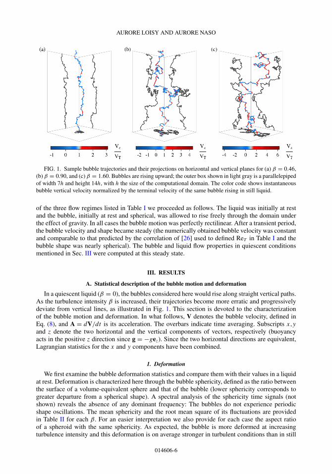
FIG. 1. Sample bubble trajectories and their projections on horizontal and vertical planes for (a) β = 0.46,(b) β = 0.90, and (c) β = 1.60. Bubbles are rising upward; the outer box shown in light gray is a parallelepipedof width 7h and height 14h, with h the size of the computational domain. The color code shows instantaneousbubble vertical velocity normalized by the terminal velocity of the same bubble rising in still liquid.

of the three flow regimes listed in Table I we proceeded as follows. The liquid was initially at restand the bubble, initially at rest and spherical, was allowed to rise freely through the domain underthe effect of gravity. In all cases the bubble motion was perfectly rectilinear. After a transient period,the bubble velocity and shape became steady (the numerically obtained bubble velocity was constantand comparable to that predicted by the correlation of [26] used to defined ReT in Table I and thebubble shape was nearly spherical). The bubble and liquid flow properties in quiescent conditionsmentioned in Sec. III were computed at this steady state.

III. RESULTS

A. Statistical description of the bubble motion and deformation

In a quiescent liquid (β = 0), the bubbles considered here would rise along straight vertical paths.As the turbulence intensity β is increased, their trajectories become more erratic and progressivelydeviate from vertical lines, as illustrated in Fig. 1. This section is devoted to the characterizationof the bubble motion and deformation. In what follows, V denotes the bubble velocity, defined inEq. (8), and A = dV/dt is its acceleration. The overbars indicate time averaging. Subscripts x,y

and z denote the two horizontal and the vertical components of vectors, respectively (buoyancyacts in the positive z direction since g = −gez). Since the two horizontal directions are equivalent,Lagrangian statistics for the x and y components have been combined.

1. Deformation

We first examine the bubble deformation statistics and compare them with their values in a liquidat rest. Deformation is characterized here through the bubble sphericity, defined as the ratio betweenthe surface of a volume-equivalent sphere and that of the bubble (lower sphericity corresponds togreater departure from a spherical shape). A spectral analysis of the sphericity time signals (notshown) reveals the absence of any dominant frequency: The bubbles do not experience periodicshape oscillations. The mean sphericity and the root mean square of its fluctuations are providedin Table II for each β. For an easier interpretation we also provide for each case the aspect ratioof a spheroid with the same sphericity. As expected, the bubble is more deformed at increasingturbulence intensity and this deformation is on average stronger in turbulent conditions than in still

014606-6

INTERACTION BETWEEN A LARGE BUOYANT BUBBLE . . .

TABLE II. Bubble deformation in quiescent (subscript T ) and turbulent conditions (in that caseoverbars indicate time averaging and the numbers in parentheses correspond to the root-mean-squarefluctuations around this mean value): �, bubble sphericity, defined as the ratio between the surfaceof a volume-equivalent sphere and that of the bubble, and χ eq, aspect ratio of an oblate spheroid withsphericity �.

β �T � χeqT χ eq

0.46 0.9944 0.9918 (±0.0031) 1.19 1.23 (−0.05,+0.05)0.90 0.9946 0.9919 (±0.0040) 1.19 1.23 (−0.07,+0.06)1.60 0.9948 0.9869 (±0.0094) 1.18 1.31 (−0.16,+0.11)

liquid. Due to the low value of the Bond number, it nevertheless remains overall modest, the aspectratios of the equivalent spheroids always being smaller than 1.4.

2. Velocity

We now examine the statistics of the bubble velocity. Its componentwise variance and the averageof Vz are listed in Table III. The most noticeable feature here is the fact that Vz is significantlylower (by 60%–77%) than that of the same bubble in an infinite quiescent liquid. Such a reductionof the rise velocity under the effect of turbulence was already reported for much smaller bubbles[3,5,6,39–41]. In these investigations, a similar reduction in rise velocity was obtained for comparableβ. Interestingly, the velocity reduction in our simulations is maximum when β ≈ 1 (for point bubbles,both nonmonotonic [3] and monotonic [5,6] evolutions of Vz/VT with β have been reported, therebyindicating that the value of β alone is not sufficient to predict the rise velocity reduction). We findthat the variances of the vertical and horizontal components of V are of the same order. They are, upto statistical uncertainty, equal to u2

0 (the variance of the liquid velocity components in a one-phaseflow) for the lowest value of β and lower than it for β � 1.

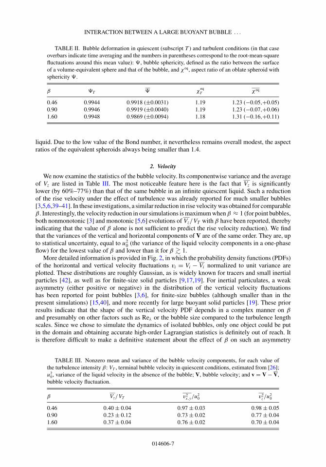
More detailed information is provided in Fig. 2, in which the probability density functions (PDFs)of the horizontal and vertical velocity fluctuations vi = Vi − Vi normalized to unit variance areplotted. These distributions are roughly Gaussian, as is widely known for tracers and small inertialparticles [42], as well as for finite-size solid particles [9,17,19]. For inertial particulates, a weakasymmetry (either positive or negative) in the distribution of the vertical velocity fluctuationshas been reported for point bubbles [3,6], for finite-size bubbles (although smaller than in thepresent simulations) [15,40], and more recently for large buoyant solid particles [19]. These priorresults indicate that the shape of the vertical velocity PDF depends in a complex manner on β

and presumably on other factors such as Reλ or the bubble size compared to the turbulence lengthscales. Since we chose to simulate the dynamics of isolated bubbles, only one object could be putin the domain and obtaining accurate high-order Lagrangian statistics is definitely out of reach. Itis therefore difficult to make a definitive statement about the effect of β on such an asymmetry

TABLE III. Nonzero mean and variance of the bubble velocity components, for each value ofthe turbulence intensity β: VT , terminal bubble velocity in quiescent conditions, estimated from [26];u2

0, variance of the liquid velocity in the absence of the bubble; V, bubble velocity; and v = V − V,bubble velocity fluctuation.

β Vz/VT v2x,y/u

20 v2

z /u20

0.46 0.40 ± 0.04 0.97 ± 0.03 0.98 ± 0.050.90 0.23 ± 0.12 0.73 ± 0.02 0.77 ± 0.041.60 0.37 ± 0.04 0.76 ± 0.02 0.70 ± 0.04

014606-7

AURORE LOISY AND AURORE NASO

− 4 − 2 0 2 410−4

10−3

10−2

10−1

100(a)

vx,y vx,y

2 1 2

PD

F

− 4 − 2 0 2 410−4

10−3

10−2

10−1

100(b)

vz vz

21 2

PD

F

β = 0.46

β = 0.90

β = 1.60

Gaussian

FIG. 2. PDFs of the (a) horizontal and (b) vertical components of the bubble velocity fluctuationsvi = Vi − Vi , normalized to unit variance. The solid black line shows the Gaussian distribution.

in the distribution of the vertical velocity fluctuations. In any case, the degree of departure from

Gaussianity in our simulations, if any, is small: We measured skewnesses |v3z /v

2z

3/2| < 0.3 and

flatnesses v4i /v

2i

2 = 3.1 ± 0.3 for i = x,y,z. Finally, although direct comparison to prior work onsmall bubbles is not possible (essentially because of the mismatch in the values of Reλ, db/L,and ReT ), it is worth mentioning that nearly Gaussian vertical velocity distributions have also beenobtained for β ≈ 0.5 [3,40] and for β ≈ 1.2 [6].

3. Acceleration

We now turn to the statistics of the bubble acceleration components. The mean bubble accelerationis zero and the componentwise acceleration variance normalized by g2 is reported in Table IV. Forany β the horizontal and vertical variances are of the same order. They depend on β: a2

i ≈ g2 for the

smallest value of β considered here, when buoyancy effects are the strongest, and a2i ≈ 10g2 for the

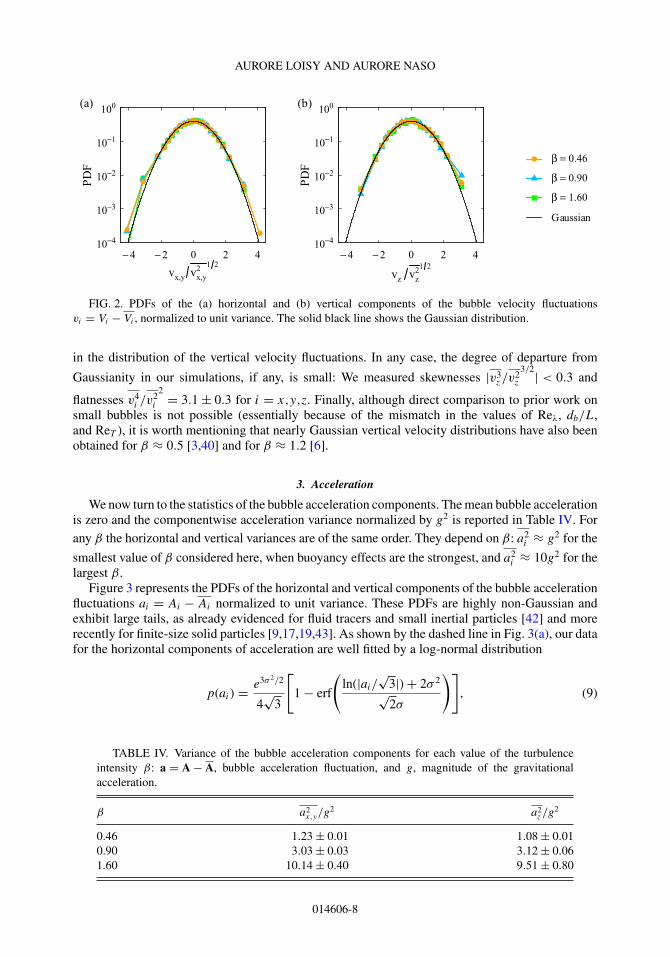
largest β.Figure 3 represents the PDFs of the horizontal and vertical components of the bubble acceleration

fluctuations ai = Ai − Ai normalized to unit variance. These PDFs are highly non-Gaussian andexhibit large tails, as already evidenced for fluid tracers and small inertial particles [42] and morerecently for finite-size solid particles [9,17,19,43]. As shown by the dashed line in Fig. 3(a), our datafor the horizontal components of acceleration are well fitted by a log-normal distribution

p(ai) = e3σ 2/2

4√

3

[1 − erf

(ln(|ai/

√3|) + 2σ 2

√2σ

)], (9)

TABLE IV. Variance of the bubble acceleration components for each value of the turbulenceintensity β: a = A − A, bubble acceleration fluctuation, and g, magnitude of the gravitationalacceleration.

β a2x,y/g

2 a2z /g

2

0.46 1.23 ± 0.01 1.08 ± 0.010.90 3.03 ± 0.03 3.12 ± 0.061.60 10.14 ± 0.40 9.51 ± 0.80

014606-8

INTERACTION BETWEEN A LARGE BUOYANT BUBBLE . . .

− 10 − 5 0 5 1010−4

10−3

10−2

10−1

100(a)

ax,y ax,y

2 1 2

PD

F

− 10 − 5 0 5 1010−4

10−3

10−2

10−1

100(b)

az az

21 2

PD

F

β = 0.46

β = 0.90

β = 1.60

Gaussian

fit

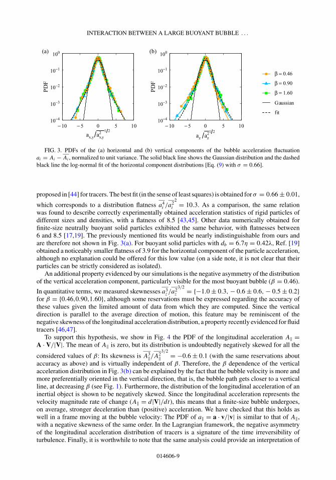
FIG. 3. PDFs of the (a) horizontal and (b) vertical components of the bubble acceleration fluctuationai = Ai − Ai , normalized to unit variance. The solid black line shows the Gaussian distribution and the dashedblack line the log-normal fit of the horizontal component distributions [Eq. (9) with σ = 0.66].

proposed in [44] for tracers. The best fit (in the sense of least squares) is obtained for σ = 0.66 ± 0.01,

which corresponds to a distribution flatness a4i /a

2i

2 = 10.3. As a comparison, the same relationwas found to describe correctly experimentally obtained acceleration statistics of rigid particles ofdifferent sizes and densities, with a flatness of 8.5 [43,45]. Other data numerically obtained forfinite-size neutrally buoyant solid particles exhibited the same behavior, with flatnesses between6 and 8.5 [17,19]. The previously mentioned fits would be nearly indistinguishable from ours andare therefore not shown in Fig. 3(a). For buoyant solid particles with db = 6.7η = 0.42λ, Ref. [19]obtained a noticeably smaller flatness of 3.9 for the horizontal component of the particle acceleration,although no explanation could be offered for this low value (on a side note, it is not clear that theirparticles can be strictly considered as isolated).

An additional property evidenced by our simulations is the negative asymmetry of the distributionof the vertical acceleration component, particularly visible for the most buoyant bubble (β = 0.46).

In quantitative terms, we measured skewnesses a3z /a

2z

3/2 = {−1.0 ± 0.3, − 0.6 ± 0.6, − 0.5 ± 0.2}for β = {0.46,0.90,1.60}, although some reservations must be expressed regarding the accuracy ofthese values given the limited amount of data from which they are computed. Since the verticaldirection is parallel to the average direction of motion, this feature may be reminiscent of thenegative skewness of the longitudinal acceleration distribution, a property recently evidenced for fluidtracers [46,47].

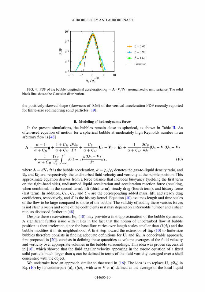
To support this hypothesis, we show in Fig. 4 the PDF of the longitudinal acceleration A‖ =A · V/|V|. The mean of A‖ is zero, but its distribution is undoubtedly negatively skewed for all the

considered values of β: Its skewness is A3‖/A

2‖

3/2 = −0.6 ± 0.1 (with the same reservations aboutaccuracy as above) and is virtually independent of β. Therefore, the β dependence of the verticalacceleration distribution in Fig. 3(b) can be explained by the fact that the bubble velocity is more andmore preferentially oriented in the vertical direction, that is, the bubble path gets closer to a verticalline, at decreasing β (see Fig. 1). Furthermore, the distribution of the longitudinal acceleration of aninertial object is shown to be negatively skewed. Since the longitudinal acceleration represents thevelocity magnitude rate of change (A‖ = d|V|/dt), this means that a finite-size bubble undergoes,on average, stronger deceleration than (positive) acceleration. We have checked that this holds aswell in a frame moving at the bubble velocity: The PDF of a‖ = a · v/|v| is similar to that of A‖,with a negative skewness of the same order. In the Lagrangian framework, the negative asymmetryof the longitudinal acceleration distribution of tracers is a signature of the time irreversibility ofturbulence. Finally, it is worthwhile to note that the same analysis could provide an interpretation of

014606-9

AURORE LOISY AND AURORE NASO

− 10 − 5 0 5 1010−4

10−3

10−2

10−1

100

A|| A||

21 2

PD

F

β = 0.46

β = 0.90

β = 1.60

Gaussian

FIG. 4. PDF of the bubble longitudinal acceleration A‖ = A · V/|V|, normalized to unit variance. The solidblack line shows the Gaussian distribution.

the positively skewed shape (skewness of 0.63) of the vertical acceleration PDF recently reportedfor finite-size sedimenting solid particles [19].

B. Modeling of hydrodynamic forces

In the present simulations, the bubbles remain close to spherical, as shown in Table II. Anoften-used equation of motion for a spherical bubble at moderately high Reynolds number in anarbitrary flow is [48]

A = α − 1

α + CM

g + 1 + CM

α + CM

DU0

Dt+ CL

α + CM

(U0 − V) × �0 + 1

α + CM

3CD

4db

|U0 − V|(U0 − V)

+ 1

α + CM

18ν

d2b

∫ t

−∞K(t − τ )

d(U0 − V)

dτdτ, (10)

where A = dV/dt is the bubble acceleration, α = ρg/ρl denotes the gas-to-liquid density ratio, andU0 and �0 are, respectively, the undisturbed fluid velocity and vorticity at the bubble position. Thisapproximate equation derives from a force balance that includes buoyancy (yielding the first termon the right-hand side), undisturbed liquid acceleration and acceleration reaction force (resulting,when combined, in the second term), lift (third term), steady drag (fourth term), and history force(last term). In addition, CM , CL, and CD are the corresponding added mass, lift, and steady dragcoefficients, respectively, and K is the history kernel. Equation (10) assumes length and time scalesof the flow to be large compared to those of the bubble. The validity of adding these various forcesis not clear a priori and some of the coefficients in it may depend on a Reynolds number and a shearrate, as discussed further in [48].

Despite these reservations, Eq. (10) may provide a first approximation of the bubble dynamics.A significant further issue with it lies in the fact that the notion of unperturbed flow at bubbleposition is then irrelevant, since the base flow varies over length scales smaller than O(db) and thebubble modifies it in its neighborhood. A first step toward the extension of Eq. (10) to finite-sizebubbles therefore consists in finding adequate definitions for U0 and �0. A conceivable approach,first proposed in [20], consists in defining these quantities as volume averages of the fluid velocityand vorticity over appropriate volumes in the bubble surroundings. This idea was proven successfulin [16], which showed that the fluid angular velocity appearing in the torque equation of a fixedsolid particle much larger than η can be defined in terms of the fluid vorticity averaged over a shellconcentric with the object.

We undertake here an approach similar to that used in [16]: The idea is to replace U0 (�0) inEq. (10) by its counterpart 〈u〉s (〈ω〉s , with ω = ∇ × u) defined as the average of the local liquid

014606-10

INTERACTION BETWEEN A LARGE BUOYANT BUBBLE . . .

velocity (vorticity) over a volume comprised between the gas-liquid interface and a surface locatedat a distance s from it. Formally, this average reads

〈q〉s(t) = 1

Vs(t)

∫V(s,t)

q(x,t)dx with Vs(t) =∫V(s,t)

dx, (11)

where V(s,t) contains the points in the liquid phase such that 0 � ψ(x,t) � s at time t , with ψ thenormal distance to the interface. If this volume-averaging approach is appropriate and if Eq. (10)provides a descent approximation of the bubble dynamics, it might be possible to find a valueof s for which the bubble acceleration A is reasonably correlated to d〈u〉s/dt , (〈u〉s − V), and(〈u〉s − V) × 〈ω〉s . Given that the adequate shell thickness s may a priori depend on the natureof the force involved, we will treat the second, third, and fourth terms on the right-hand side ofEq. (10) separately. Owing to the lack of a reliable expression of the history kernel K for a bubble innonrectilinear motion at finite Reynolds number [48], the history term cannot be treated rigorouslyand is therefore not investigated.

We first investigate the second term on the right-hand side of Eq. (10), which represents thecombination of the acceleration reaction force and the effect of the undisturbed fluid accelerationand in which the unknown variable is U0. Under the assumption of a near-spherical bubble shape,CM is constant and is unimportant for the present purpose since it only affects the force magnitudes,not their correlation with the acceleration. We will now determine the thickness sacc

u of the shellover which u should be averaged for estimating U0 at best. Recalling that part of the force arisesfrom the undisturbed fluid acceleration integrated over the bubble volume, it seems reasonable toexpect the shell volume to be comparable to it, which yields an expected value of sacc

u = 0.13db,assuming the bubble to be nearly spherical. The optimal shell thickness sacc

u has been determinedfrom our simulations by maximizing the componentwise correlation between A and Facc, the latterbeing defined by

Facc = d〈u〉saccu

dt, (12)

in which the unimportant factor (1 + CM )/(α + CM ) is omitted. The maximum correlationcoefficients were obtained for sacc

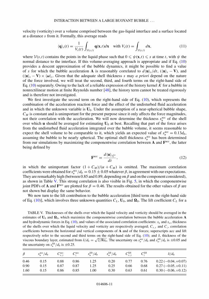
u /db = 0.15 ± 0.05 whatever β, in agreement with our expectations.They are remarkably high (between 0.85 and 0.89, depending on β and on the component considered),as shown in Table V. This strong correlation is also visible in Fig. 5, in which the componentwisejoint PDFs of A and Facc are plotted for β = 0.46. The results obtained for the other values of β arenot shown but display the same behavior.

We now turn to the lift contribution to the bubble acceleration [third term on the right-hand sideof Eq. (10)], which involves three unknown quantities CL, U0, and �0. The lift coefficient CL for a

TABLE V. Thicknesses of the shells over which the liquid velocity and vorticity should be averaged in theestimates of U0 and �0, which maximize the componentwise correlation between the bubble acceleration Aand hydrodynamic forces in Eq. (10), and values of the associated correlation coefficients: su and sω, thicknessof the shells over which the liquid velocity and vorticity are respectively averaged; Cx,y and Cz, correlationcoefficients between the horizontal and vertical components of A and of the forces; superscripts acc and liftrespectively refer to the second and third terms on the right-hand side of Eq. (10); and δ, thickness of theviscous boundary layer, estimated from δ/db = √

2/Reb. The uncertainty on saccu /db and s lift

ω /db is ±0.05 andthe uncertainty on s lift

u /db is ±0.25.

β saccu /db Cacc

x,y Caccz s lift

u /db s liftω /db C lift

x,y C liftz δ/db

0.46 0.15 0.88 0.86 1.25 0.20 0.77 0.76 0.22 (−0.04,+0.07)0.90 0.15 0.87 0.87 1.25 0.25 0.66 0.68 0.27 (−0.05,+0.11)1.60 0.15 0.86 0.85 1.00 0.30 0.63 0.61 0.30 (−0.06,+0.12)

014606-11

AURORE LOISY AND AURORE NASO

− 4 − 2 0 2 4

− 5

0

5

Fx,yacc

Ax,

y

− 4 − 2 0 2 4

− 5

0

5

Fzacc

Az

−6

−5

−4

−3

−2

−1

log10 PDF(Ai,Fi)

FIG. 5. Componentwise joint PDFs (logarithmic grayscale) of the bubble acceleration A andFacc = d〈u〉sacc

u/dt , for β = 0.46. The value of sacc

u is given in Table V.

spherical bubble depends a priori on the Reynolds number, the shear rate, and possibly other factors[49,50], but will be assumed to be constant in the results presented hereafter (we have checked thatusing the expression of CL proposed by [49], which includes dependences on Reynolds numberand shear rate, yields identical results). Under this assumption, its exact value is unimportant forthe present purpose. The optimal shell thicknesses s lift

u and s liftω are determined by maximizing the

correlation between A and Flift, the latter being defined by

Flift = (〈u〉sliftu

− V) × 〈ω〉slift

ω, (13)

in which the unimportant factor CL/(α + CM ) is omitted. The results are summarized in Table V.The largest correlation coefficients are approximately {0.8,0.7,0.6} for β = {0.46,0.90,1.60}. Theywere obtained by estimating U0 as the volume average of velocity over distances O(db) from theinterface and �0 as the volume average of vorticity over smaller volumes of liquid, more preciselyover distances O(δ), where δ is the thickness of a loosely defined “boundary layer,” estimated asδ/db ∼ √

2/Reb [51], where Reb is the bubble Reynolds number defined as Reb = |〈u〉sliftu

− V|db/ν

(removing the time average in the definition of Reb does not affect the results). Incidentally, theundisturbed fluid vorticity entering in the torque equation of a large solid particle in turbulence wasfound to be well estimated by averaging vorticity in the same volume (up to distances ∼ δ fromthe particle surface) [16]. The reasonable correlation between A and Flift when s lift

u and s liftω have

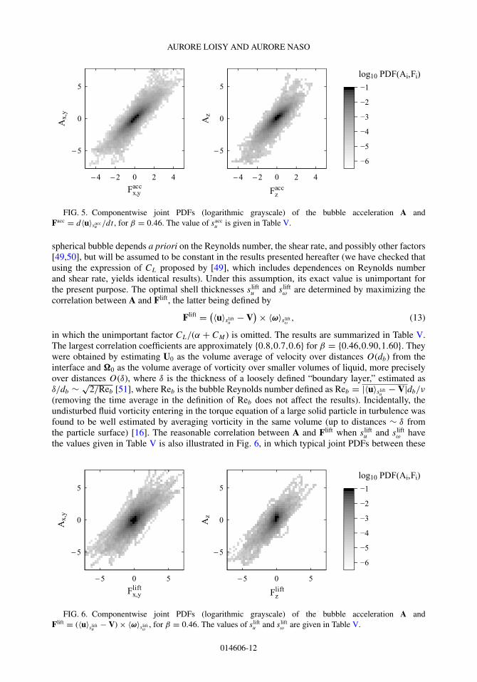
the values given in Table V is also illustrated in Fig. 6, in which typical joint PDFs between these

− 5 0 5

− 5

0

5

Fx,ylift

Ax,

y

− 5 0 5

− 5

0

5

Fzlift

Az

−6

−5

−4

−3

−2

−1

log10 PDF(Ai,Fi)

FIG. 6. Componentwise joint PDFs (logarithmic grayscale) of the bubble acceleration A andFlift = (〈u〉slift

u− V) × 〈ω〉slift

ω, for β = 0.46. The values of s lift

u and s liftω are given in Table V.

014606-12

INTERACTION BETWEEN A LARGE BUOYANT BUBBLE . . .

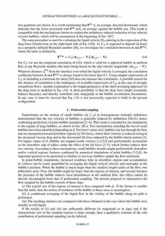
two quantities are shown. It is worth mentioning that Flift is, on average, directed downward, whichindicates that the force associated with Flift acts, on average, against the bubble rise. This result iscompatible with the mechanisms known to explain the turbulence-induced reduction of rise velocityof point bubbles, which will be summarized at the beginning of Sec. III C.

The same procedure is used for evaluating the liquid velocity U0 entering in the expression of thedrag force [fourth term on the right-hand side of Eq. (10)]. As CD is expected to depend (at least)on a (properly defined) Reynolds number [48], we investigate the correlation between A and Fdrag,where the latter is defined by

Fdrag = CD|〈u〉s

dragu

− V|(〈u〉s

dragu

− V). (14)

For CD we use the empirical correlation of [26], which is valid for a spherical bubble in uniformflow at any Reynolds number (the latter being based on the slip velocity magnitude |〈u〉

sdragu

− V|).Whatever distance s

dragu from the interface over which the liquid velocity is averaged, the correlation

coefficient between A and Fdrag is always found to be lower than 0.1. Using simpler expressions ofCD or including a correction for shear [48] does not increase this correlation. A possible reason forthis absence of correlation is the inadequacy of available expressions of CD in the case of stronglynonuniform flows. Another explanation is the inappropriateness of the shell-averaging approach forthe drag term as modeled in Eq. (10). A third possibility is that the drag force might essentiallybalance buoyancy and thereby contribute only marginally to the bubble acceleration fluctuations.In any case, it must be stressed that Eq. (10) is not necessarily expected to hold in the presentconfiguration.

C. Preferential sampling

Experiments on the motion of small bubbles (db � η) in homogeneous isotropic turbulencedemonstrated that the rise velocity of bubbles is generally reduced by turbulence [40,41], henceconfirming predictions of point-bubble simulations [1–6]. This result is extended by our simulationsto the regime of large bubbles, as shown in Sec. III A. Two mechanisms retarding the rise of smallbubbles have been identified depending on β. For lower values of β, bubbles rise fast through the flowand are transported toward downflow regions by lift forces, where their velocity is reduced owing tothe increased viscous drag and to the downward lift force induced by the bubble lateral motion [3].For higher values of β, bubbles are trapped inside vortices [1,2,52] and preferentially accumulateon the downflow side of eddies under the effect of the lift force [3–5], which further reduces theirrise velocity. According to these mechanisms, small bubbles should sample preferentially downflowand/or vortical regions, features confirmed by numerical simulations of point bubbles [3,5,6]. Animportant question to be answered is whether or not large bubbles sample the flow uniformly.

In point-bubble simulations, increased residence time in downflow regions and accumulationin vortices can be easily quantified by averaging the liquid vertical velocity and enstrophy at thebubble’s position. When the bubble is much larger than the smallest length scales of the flow, twodifficulties arise: First, the bubble might be larger than the regions of interest, and second, becausethe presence of the bubble induces local disturbances in the ambient flow, this effect cannot bedirectly disentangled from that of preferential sampling. The present proposal to characterize theflow sampled by the bubble consists of three steps.

(i) The typical size of the regions of interest is first compared with db. If the former is smallerthan the latter, then the notion of residence of the bubble in these areas is meaningless.

(ii) A conditional averaging of the liquid flow in the vicinity of the bubble along its path isperformed.

(iii) The resulting statistics are compared with those obtained in the case where the bubble risessteadily in still liquid.

If the results of (ii) and (iii) are sufficiently different (in magnitude or in sign) and if thecharacteristic size of the sampled regions is large enough, then a qualitative estimate of the solecontribution of preferential sampling can be inferred.

014606-13

AURORE LOISY AND AURORE NASO

(b)

0

1

2

3

4

5|ω|

|ω|0

(a)

−3

−2

−1

0

1

2

3uz

u0

(c)

−1

0

1sgn(D)

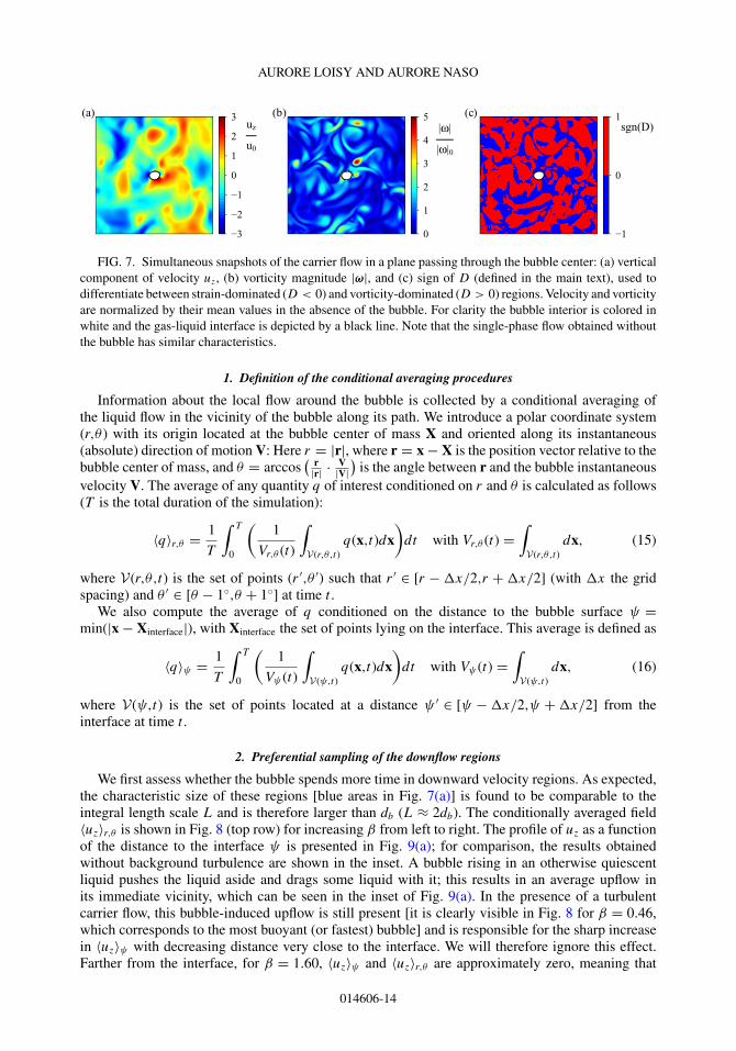
FIG. 7. Simultaneous snapshots of the carrier flow in a plane passing through the bubble center: (a) verticalcomponent of velocity uz, (b) vorticity magnitude |ω|, and (c) sign of D (defined in the main text), used todifferentiate between strain-dominated (D < 0) and vorticity-dominated (D > 0) regions. Velocity and vorticityare normalized by their mean values in the absence of the bubble. For clarity the bubble interior is colored inwhite and the gas-liquid interface is depicted by a black line. Note that the single-phase flow obtained withoutthe bubble has similar characteristics.

1. Definition of the conditional averaging procedures

Information about the local flow around the bubble is collected by a conditional averaging ofthe liquid flow in the vicinity of the bubble along its path. We introduce a polar coordinate system(r,θ ) with its origin located at the bubble center of mass X and oriented along its instantaneous(absolute) direction of motion V: Here r = |r|, where r = x − X is the position vector relative to thebubble center of mass, and θ = arccos

( r|r| · V

|V|)

is the angle between r and the bubble instantaneousvelocity V. The average of any quantity q of interest conditioned on r and θ is calculated as follows(T is the total duration of the simulation):

〈q〉r,θ = 1

T

∫ T

0

(1

Vr,θ (t)

∫V(r,θ,t)

q(x,t)dx)

dt with Vr,θ (t) =∫V(r,θ,t)

dx, (15)

where V(r,θ,t) is the set of points (r ′,θ ′) such that r ′ ∈ [r − �x/2,r + �x/2] (with �x the gridspacing) and θ ′ ∈ [θ − 1◦,θ + 1◦] at time t .

We also compute the average of q conditioned on the distance to the bubble surface ψ =min(|x − Xinterface|), with Xinterface the set of points lying on the interface. This average is defined as

〈q〉ψ = 1

T

∫ T

0

(1

Vψ (t)

∫V(ψ,t)

q(x,t)dx)

dt with Vψ (t) =∫V(ψ,t)

dx, (16)

where V(ψ,t) is the set of points located at a distance ψ ′ ∈ [ψ − �x/2,ψ + �x/2] from theinterface at time t .

2. Preferential sampling of the downflow regions

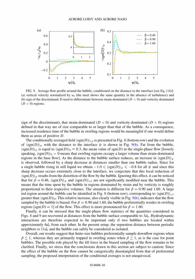
We first assess whether the bubble spends more time in downward velocity regions. As expected,the characteristic size of these regions [blue areas in Fig. 7(a)] is found to be comparable to theintegral length scale L and is therefore larger than db (L ≈ 2db). The conditionally averaged field〈uz〉r,θ is shown in Fig. 8 (top row) for increasing β from left to right. The profile of uz as a functionof the distance to the interface ψ is presented in Fig. 9(a); for comparison, the results obtainedwithout background turbulence are shown in the inset. A bubble rising in an otherwise quiescentliquid pushes the liquid aside and drags some liquid with it; this results in an average upflow inits immediate vicinity, which can be seen in the inset of Fig. 9(a). In the presence of a turbulentcarrier flow, this bubble-induced upflow is still present [it is clearly visible in Fig. 8 for β = 0.46,which corresponds to the most buoyant (or fastest) bubble] and is responsible for the sharp increasein 〈uz〉ψ with decreasing distance very close to the interface. We will therefore ignore this effect.Farther from the interface, for β = 1.60, 〈uz〉ψ and 〈uz〉r,θ are approximately zero, meaning that

014606-14

INTERACTION BETWEEN A LARGE BUOYANT BUBBLE . . .

r db

rd b

0 1 2−2

−1

0

1

2 β = 0.46

r db0 1 2

β = 0.90

r db0 1 2

β = 1.60

−0.3

−0.2

−0.1

0.0

0.1

0.2

0.3

<uz>r,θ u0

r db

rd b

0 1 2−2

−1

0

1

2 β = 0.46

r db0 1 2

β = 0.90

r db0 1 2

β = 1.60

0.1

0.2

0.3

0.4

0.5

0.6<sgn(D)>r,θ

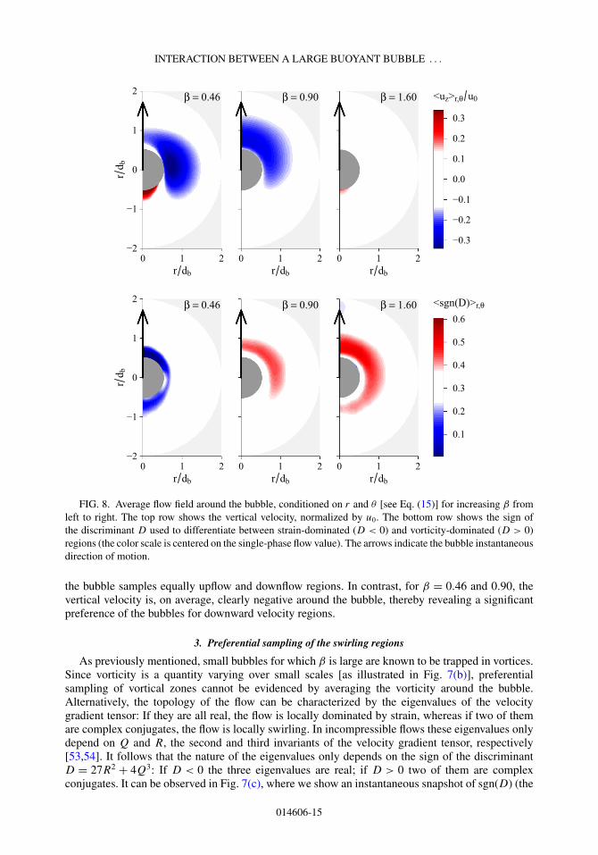
FIG. 8. Average flow field around the bubble, conditioned on r and θ [see Eq. (15)] for increasing β fromleft to right. The top row shows the vertical velocity, normalized by u0. The bottom row shows the sign ofthe discriminant D used to differentiate between strain-dominated (D < 0) and vorticity-dominated (D > 0)regions (the color scale is centered on the single-phase flow value). The arrows indicate the bubble instantaneousdirection of motion.

the bubble samples equally upflow and downflow regions. In contrast, for β = 0.46 and 0.90, thevertical velocity is, on average, clearly negative around the bubble, thereby revealing a significantpreference of the bubbles for downward velocity regions.

3. Preferential sampling of the swirling regions

As previously mentioned, small bubbles for which β is large are known to be trapped in vortices.Since vorticity is a quantity varying over small scales [as illustrated in Fig. 7(b)], preferentialsampling of vortical zones cannot be evidenced by averaging the vorticity around the bubble.Alternatively, the topology of the flow can be characterized by the eigenvalues of the velocitygradient tensor: If they are all real, the flow is locally dominated by strain, whereas if two of themare complex conjugates, the flow is locally swirling. In incompressible flows these eigenvalues onlydepend on Q and R, the second and third invariants of the velocity gradient tensor, respectively[53,54]. It follows that the nature of the eigenvalues only depends on the sign of the discriminantD = 27R2 + 4Q3: If D < 0 the three eigenvalues are real; if D > 0 two of them are complexconjugates. It can be observed in Fig. 7(c), where we show an instantaneous snapshot of sgn(D) (the

014606-15

AURORE LOISY AND AURORE NASO

ψ db0 1 2 3 4 5

0.1

0.2

0.3

0.4

0.5(b)

<sgn

(D)>

ψ

β = 0.46β = 0.90β = 1.60

ψ db0 1 2 3 4 5

−0.2

0

0.2

0.4

0.6

(a)

<uz>

ψu 0

0 1 2

0

0.5

FIG. 9. Average flow profile around the bubble, conditioned on the distance to the interface [see Eq. (16)]:(a) vertical velocity normalized by u0 (the inset shows the same quantity in the absence of turbulence) and(b) sign of the discriminant D used to differentiate between strain-dominated (D < 0) and vorticity-dominated(D > 0) regions.

sign of the discriminant), that strain-dominated (D < 0) and vorticity-dominated (D > 0) regionsdefined in that way are of size comparable to or larger than that of the bubble. As a consequence,increased residence time of the bubble in swirling regions would be meaningful if one would definethem as areas of positive D.

The conditionally averaged field 〈sgn(D)〉r,θ is presented in Fig. 8 (bottom row) and the evolutionof 〈sgn(D)〉ψ with the distance to the interface ψ is shown in Fig. 9(b). Far from the bubble,〈sgn(D)〉ψ is equal to 〈sgn(D)〉0 ≈ 0.3, the mean value of sgn(D) in the single-phase flow [looselyspeaking, 〈sgn(D)〉0 > 0 means that swirling regions occupy a larger volume than strain-dominatedregions in the base flow]. As the distance to the bubble surface reduces, an increase in 〈sgn(D)〉ψis observed, followed by a sharp decrease at distances smaller than one bubble radius. Since fora single bubble rising in still liquid we obtain −1.0 � 〈sgn(D)〉ψ � −0.8 for all ψ and since thissharp decrease occurs extremely close to the interface, we conjecture that this local reduction of〈sgn(D)〉ψ results from the distortion of the flow by the bubble. Ignoring this effect, it can be noticedthat for β = 0.46, 〈sgn(D)〉ψ and 〈sgn(D)〉r,θ are not significantly modified near the bubble. Thismeans that the time spent by the bubble in regions dominated by strain and by vorticity is roughlyproportional to their respective volumes. The situation is different for β = 0.90 and 1.60. A largered region around the bubble can be identified in Fig. 8 (bottom row), corresponding to 〈sgn(D)〉r,θgreater than 〈sgn(D)〉0. This relative increase, also clearly visible in Fig. 9(b), indicates that the flowsampled by the bubble is biased: For β = 0.90 and 1.60, the bubble preferentially resides in swirlingregions [sgn(D) = 1] of the flow. This effect is more pronounced for β = 1.60.

Finally, it can be stressed that the single-phase flow statistics of the quantities considered inFigs. 8 and 9 are recovered at distances from the bubble surface comparable to 3db. Hydrodynamicinteractions are therefore expected to be important only if two bubbles are located withinapproximately 6db from each other. In the present setup, the separation distance between periodicneighbors is 11db and the bubble can safely be considered as isolated.

Overall, our results suggest that finite-size bubbles preferentially sample downflow regions whenβ � 1, whereas they are primarily trapped in swirling zones when β � 1, as is the case for pointbubbles. The possible role played by the lift force in the biased sampling of the flow remains to beclarified. Finally, we stress that the conclusions drawn in this section are subject to caution: Sincethe effect of the bubble on the flow cannot be categorically disentangled from that of preferentialsampling, the proposed interpretation of the conditional averages is not unequivocal.

014606-16

INTERACTION BETWEEN A LARGE BUOYANT BUBBLE . . .

IV. CONCLUSION

Interface-resolved numerical simulations of the rise of an isolated finite-size bubble in otherwisehomogeneous isotropic turbulence were carried out for different values of the turbulence intensityβ, defined as the root mean square of the liquid velocity fluctuations divided by the terminal velocityof the bubble in still liquid. These simulations were run over a time period long enough to allow areasonable convergence of bubble Lagrangian and liquid Eulerian statistics.

The bubble kinematics was first characterized. Turbulence was found to drastically reduce its risevelocity, a property already known for microbubbles. Acceleration statistics display some featuressimilar to those of fluid tracers, small inertial particles, and finite-size rigid objects. In particular,the bubble horizontal acceleration distribution is well fitted by a log-normal distribution. The PDFof the vertical component is negatively skewed, as a consequence of the preferential alignmentof the bubble velocity with gravity and of the negative asymmetry of its longitudinal accelerationPDF. This latter property means that the bubble undergoes on average stronger deceleration thanpositive acceleration and had been previously evidenced for fluid tracers only (in that case it isrelated to the time irreversibility of turbulence). Then a physically relevant definition of the liquidflow experienced by the bubble, as it enters in usual models of the liquid acceleration force andof the lift force, was proposed. Our aim was not to propose a complete and accurate equation ofmotion of the bubble, but rather to propose some reasonable estimates of the liquid velocity andvorticity that enter in the definition of at least some of the typical forces known to act on inclusionssuspended in simple flows. We think this approach opens alternative ways for the design of models ofthe dynamics of finite-size particles in turbulence, although it is still at a preliminary stage. Finally,the present simulations show that the behavior of a bubble much larger than the Kolmogorov scaleis qualitatively similar to that of a small bubble in terms of preferential sampling of the turbulentflow. In particular, conditional averaging of the liquid flow in the bubble vicinity suggests that whenβ � 1 the bubble is more likely to reside in downflow regions of large extent, whereas when β � 1the bubble has a preference for swirling zones. Underlying mechanisms, however, still need to beelucidated.

The results presented in this paper were obtained at rather low Taylor Reynolds number and shouldbe confirmed for higher values of it. However, previous investigations carried out at similar Reλ haveshed some light on the interaction between finite-size solid objects and turbulence [16,17]. The goodqualitative agreement between our results and those known for small bubbles at Reλ = O(100) isalso very encouraging.

The above results were obtained using a turbulence forcing that consists in including a bodyforce proportional to liquid velocity in the momentum conservation equation. As a further validationstep, it would be desirable to reproduce the present simulations using a different forcing scheme. Apossible alternative is the random forcing of [55] used in, e.g., the simulation of interface-resolvedparticle-laden flow [56].

ACKNOWLEDGMENTS

The authors would like to thank Peter Spelt for enlightening discussions and for helpfulsuggestions on this manuscript. This research was partially funded by the French research agency(Grant No. ANR-12-BS09-0011) and was performed using the HPC resources provided byGENCI-CINES and GENCI-IDRIS (Grant No. x20162b6893), PSMN (Ecole Normale Superieurede Lyon), P2CHPD (Universite Claude Bernard Lyon 1), and PMCS2I (Ecole Centrale de Lyon).

[1] L.-P. Wang and M. R. Maxey, The motion of microbubbles in a forced isotropic and homogeneousturbulence, Appl. Sci. Res. 51, 291 (1993).

014606-17

AURORE LOISY AND AURORE NASO

[2] M. R. Maxey, E. J. Chang, and L.-P. Wang, Simulation of interactions between microbubbles and turbulentflows, Appl. Mech. Rev. 47, S70 (1994).

[3] P. D. M. Spelt and A. Biesheuvel, On the motion of gas bubbles in homogeneous isotropic turbulence,J. Fluid Mech. 336, 221 (1997).

[4] I. M. Mazzitelli, D. Lohse, and F. Toschi, The effect of microbubbles on developed turbulence,Phys. Fluids 15, L5 (2003).

[5] I. M. Mazzitelli, D. Lohse, and F. Toschi, On the relevance of the lift force in bubbly turbulence, J. FluidMech. 488, 283 (2003).

[6] M. R. Snyder, O. M. Knio, J. Katz, and O. P. Le Maıtre, Statistical analysis of small bubble dynamics inisotropic turbulence, Phys. Fluids 19, 065108 (2007).

[7] S. Balachandar and J. K. Eaton, Turbulent dispersed multiphase flow, Annu. Rev. Fluid Mech. 42, 111(2010).

[8] R. Volk, E. Calzavarini, E. Leveque, and J.-F. Pinton, Dynamics of inertial particles in a turbulent vonKarman flow, J. Fluid Mech. 668, 223 (2011).

[9] R. Zimmermann, Y. Gasteuil, M. Bourgoin, R. Volk, A. Pumir, and J.-F. Pinton, Rotational Intermittencyand Turbulence Induced Lift Experienced by Large Particles in a Turbulent Flow, Phys. Rev. Lett. 106,154501 (2011).

[10] G. Bellani and E. A. Variano, Slip velocity of large neutrally buoyant particles in turbulent flows, New J.Phys. 14, 125009 (2012).

[11] G. Bellani, M. L. Byron, A. G. Collignon, C. R. Meyer, and E. A. Variano, Shape effects on turbulentmodulation by large nearly neutrally buoyant particles, J. Fluid Mech. 712, 41 (2012).

[12] S. Klein, M. Gibert, A. Berut, and E. Bodenschatz, Simultaneous 3D measurement of the translation androtation of finite-size particles and the flow field in a fully developed turbulent water flow, Meas. Sci.Technol. 24, 024006 (2013).

[13] V. Mathai, V. N. Prakash, J. Brons, C. Sun, and D. Lohse, Wake-Driven Dynamics of Finite-Sized BuoyantSpheres in Turbulence, Phys. Rev. Lett. 115, 124501 (2015).

[14] F. Ravelet, C. Colin, and F. Risso, On the dynamics and breakup of a bubble rising in a turbulent flow,Phys. Fluids 23, 1 (2011).

[15] V. N. Prakash, Y. Tagawa, E. Calzavarini, J. M. Mercado, F. Toschi, D. Lohse, and C. Sun, How gravityand size affect the acceleration statistics of bubbles in turbulence, New J. Phys. 14, 105017 (2012).

[16] A. Naso and A. Prosperetti, The interaction between a solid particle and a turbulent flow, New J. Phys.12, 033040 (2010).

[17] H. Homann and J. Bec, Finite-size effects in the dynamics of neutrally buoyant particles in turbulent flow,J. Fluid Mech. 651, 81 (2010).

[18] M. Cisse, H. Homann, and J. Bec, Slipping motion of large neutrally buoyant particles in turbulence,J. Fluid Mech. 735, R1 (2013).

[19] A. Chouippe and M. Uhlmann, Forcing homogeneous turbulence in direct numerical simulation ofparticulate flow with interface resolution and gravity, Phys. Fluids 27, 123301 (2015).

[20] A. Merle, D. Legendre, and J. Magnaudet, Forces on a high-Reynolds-number spherical bubble in aturbulent flow, J. Fluid Mech. 532, 53 (2005).

[21] D. Legendre, A. Merle, and J. Magnaudet, Wake of a spherical bubble or a solid sphere set fixed in aturbulent environment, Phys. Fluids 18, 048102 (2006).

[22] J. Lu and G. Tryggvason, Numerical study of turbulent bubbly downflows in a vertical channel,Phys. Fluids 18, 103302 (2006).

[23] I. A. Bolotnov, K. E. Jansen, D. A. Drew, A. A. Oberai, R. T. Lahey, Jr., and M. Z. Podowski, Detacheddirect numerical simulations of turbulent two-phase bubbly channel flow, Int. J. Multiphase Flow 37, 647(2011).

[24] J. Lu and G. Tryggvason, Dynamics of nearly spherical bubbles in a turbulent channel upflow, J. FluidMech. 732, 166 (2013).

[25] S. Dabiri, J. Lu, and G. Tryggvason, Transition between regimes of a vertical channel bubbly upflow dueto bubble deformability, Phys. Fluids 25, 102110 (2013).

014606-18

INTERACTION BETWEEN A LARGE BUOYANT BUBBLE . . .

[26] R. Mei, J. F. Klausner, and C. J. Lawrence, A note on the history force on a spherical bubble at finiteReynolds number, Phys. Fluids 6, 418 (1994).

[27] A. Chorin, Numerical solution of the Navier-Stokes equations, Math. Comput. 22, 745 (1968).[28] M. Sussman, P. Smereka, and S. Osher, A level set approach for computing solutions to incompressible

two-phase flow, J. Comput. Phys. 114, 146 (1994).[29] V. Sabelnikov, A. Y. Ovsyannikov, and M. Gorokhovski, Modified level set equation and its numerical

assessment, J. Comput. Phys. 278, 1 (2014).[30] J. U. Brackbill, D. B. Kothe, and C. Zemach, A continuum method for modeling surface tension,

J. Comput. Phys. 100, 335 (1992).[31] G. Russo and P. Smereka, A remark on computing distance functions, J. Comput. Phys. 163, 51 (2000).[32] M. Sussman and S. Uto, A computational study of the spreading of oil underneath a sheet of ice, CAM

Report 98-32 (University of California, Los Angeles, 1998).[33] A. Loisy, A. Naso, and P. D. M. Spelt, Buoyancy-driven bubbly flows: ordered and free rise at small and

intermediate volume fraction, J. Fluid Mech. (to be published).[34] Z. Amoura, V. Roig, F. Risso, and A.-M. Billet, Attenuation of the wake of a sphere in an intense incident

turbulence with large length scales, Phys. Fluids 22, 055105 (2010).[35] I. Eames, P. B. Johnson, V. Roig, and F. Risso, Effect of turbulence on the downstream velocity deficit of

a rigid sphere, Phys. Fluids 23, 095103 (2011).[36] T. S. Lundgren, Linearly forced isotropic turbulence, Annual Research Briefs (Center for Turbulence

Research, Stanford, 2003), pp. 461–473.[37] C. Rosales and C. Meneveau, Linear forcing in numerical simulations of isotropic turbulence: Physical

space implementations and convergence properties, Phys. Fluids 17, 095106 (2005).[38] B. Duret, G. Luret, J. Reveillon, T. Menard, A. Berlemont, and F. X. Demoulin, DNS analysis of turbulent

mixing in two-phase flows, Int. J. Multiphase Flow 40, 93 (2012).[39] J. C. R. Fung, Gravitational settling of particles and bubbles in homogeneous turbulence, J. Geophys. Res.

98, 20287 (1993).[40] R. E. G. Poorte and A. Biesheuvel, Experiments on the motion of gas bubbles in turbulence generated by

an active grid, J. Fluid Mech. 461, 127 (2002).[41] A. Aliseda and J. C. Lasheras, Preferential concentration and rise velocity reduction of bubbles immersed

in a homogeneous and isotropic turbulent flow, Phys. Fluids 23, 093301 (2011).[42] F. Toschi and E. Bodenschatz, Lagrangian properties of particles in turbulence, Annu. Rev. Fluid Mech.

41, 375 (2009).[43] N. M. Qureshi, U. Arrieta, C. Baudet, A. Cartellier, Y. Gagne, and M. Bourgoin, Acceleration statistics of

inertial particles in turbulent flow, Eur. Phys. J. B 66, 531 (2008).[44] N. Mordant, A. M. Crawford, and E. Bodenschatz, Three-Dimensional Structure of the Lagrangian

Acceleration in Turbulent Flows, Phys. Rev. Lett. 93, 214501 (2004).[45] N. M. Qureshi, M. Bourgoin, C. Baudet, A. Cartellier, and Y. Gagne, Turbulent Transport of Material

Particles: An Experimental Study of Finite Size Effects, Phys. Rev. Lett. 99, 184502 (2007).[46] E. Leveque and A. Naso, Introduction of longitudinal and transverse Lagrangian velocity increments in

homogeneous and isotropic turbulence, Europhys. Lett. 108, 54004 (2014).[47] H. Xu, A. Pumir, G. Falkovich, E. Bodenschatz, M. Shats, H. Xia, N. Francois, and G. Boffetta, Flight-crash

events in turbulence, Proc. Natl. Acad. Sci. USA 111, 7558 (2014).[48] J. Magnaudet and I. Eames, The motion of high-Reynolds-number bubbles in inhomogeneous flows,

Annu. Rev. Fluid Mech. 32, 659 (2000).[49] D. Legendre and J. Magnaudet, The lift force on a spherical bubble in a viscous linear shear flow, J. Fluid

Mech. 368, 81 (1998).[50] M. Rastello, J.-L. Marie, and M. Lance, Drag and lift forces on clean spherical and ellipsoidal bubbles in

a solid-body rotating flow, J. Fluid Mech. 682, 434 (2011).[51] D. W. Moore, The boundary layer on a spherical gas bubble, J. Fluid Mech. 16, 161 (1963).[52] K. J. Sene, J. C. R. Hunt, and N. H. Thomas, The role of coherent structures in bubble transport by

turbulent shear flows, J. Fluid Mech. 259, 219 (1994).

014606-19

AURORE LOISY AND AURORE NASO

[53] B. J. Cantwell, Exact solution of a restricted Euler equation for the velocity gradient tensor, Phys. FluidsA 4, 782 (1992).

[54] A. Naso and A. Pumir, Scale dependence of the coarse-grained velocity derivative tensor structure inturbulence, Phys. Rev. E 72, 056318 (2005).

[55] K. Alvelius, Random forcing of three-dimensional homogeneous turbulence, Phys. Fluids 11, 1880 (1999).[56] A. Ten Cate, J. J. Derksen, L. M. Portela, and H. E. A. van den Akker, Fully resolved simulations of

colliding monodisperse spheres in forced isotropic turbulence, J. Fluid Mech. 519, 233 (2004).

014606-20