intelligent design objects applied to the spatial ...etd.lib.metu.edu.tr/upload/12617003/index.pdf · INTELLIGENT DESIGN OBJECTS APPLIED TO THE SPATIAL ALLOCATION ... layout organization

INTELLIGENT DESIGN OBJECTS APPLIED TO THE SPATIAL ALLOCATION PROBLEM

A THESIS SUBMITED TO THE GRADUATE SCHOOL OF NATURAL AND APPLIED SCIENCES

OF MIDDLE EAST TECHNICAL UNIVERSITY

BY

JAVIER I. ZARATIEGUI FERNANDEZ

IN PARTIAL FULFILLMENT OF THE REQUIREMENTS FOR

THE DEGREE OF MASTER OF SCIENCE IN

COMPUTATIONAL DESIGN AND FABRICATION TECHNOLOGIES IN

ARCHITECTURE

MARCH 2014

Approval of the thesis:

INTELLIGENT DESIGN OBJECTS APPLIED TO THE SPATIAL

ALLOCATION PROBLEM.

submitted by JAVIER I. ZARATIEGUI FERNÁNDEZ in partial fulfillment of the

requirements for the degree of Master of Science in Computational Design and

Fabrication Technologies in Architecture in Architecture Department, Middle

East Technical University by,

Prof. Dr. Canan Özgen

Dean, Graduate School of Natural and Applied Sciences

Prof. Dr. Güven Arif Sargın

Head of Department, Architecture

Assoc. Prof. Dr. Arzu Gönenç Sorguç

Supervisor, Architecture Department, METU

Examining Committee Members:

Prof. Dr. Ahmet Can Baykan

Architecture Department, METU

Assoc. Prof. Dr. Arzu Gönenç Sorguç


Assist. Prof. Dr. Başak Uçar Kırmızıgül

Architecture Department, TED University

Assoc. Prof. Dr. Ali Murat Tanyer


Dr. Mehmet Koray Pekeriçli


Date: 07/02/2014

iv

I hereby declare that all information in this document has been obtained and

presented in accordance with academic rules and ethical conduct. I also

declare that, as required by these rules and conduct, I have fully cited and

referenced all material and results that are not original to this work

Name, Last Name: JAVIER IGNACIO

ZARATIEGUI FERNÁNDEZ

Signature:

v

ABSTRACT

INTELLIGENT DESIGN OBJECTS APPLIED TO THE SPATIAL

ALLOCATION PROBLEM.

Zaratiegui Fernández, Javier Ignacio.

M.Sc., Computational Design and Fabrication Technologies in Architecture.

Supervisor: Assoc. Prof. Dr. Arzu Gönenç Sorguç.

March 2014, 80 pages.

This thesis approaches the spatial allocation problem as a multi-objective

optimization problem. It proposes the use of Intelligent Design Objects (IDO)

model to help designers with this task. Solutions are generated and evaluated,

according the user defined criteria. Iterative improvement is proposed as a help to

visualize candidate solutions and conceive the desired spatial relations. By

defining the criteria and rating it numerically, both designer and client are able

compare the solutions obtained. The use of fuzzy logic is implemented to address

soft concepts as part of the architectural design process. New relations are defined

until a good solution is found. The implementation is evaluated via two case

studies: layout organization of sets of rectangles (two dimensions) and TUDelft

graduation project for the American Embassy in The Hague (three dimensions).

Keywords: Spatial allocation, Intelligent Design Objects, Building layout,

Optimization, Multi-objective, Genetic algorithm, Fuzzy logic.

vi

ÖZ

MEKANSAL KURGU PROBLEMİNE AKILLI TASARIM OBJELERİ

UYGULAMASI

Zaratiegui Fernández, Javier Ignacio

Yüksek Lisans, Mimarlıkta Sayısal Tasarım ve Üretim Teknolojileri

Tez Yöneticisi: Doç. Dr. Arzu Gönenç Sorguç.

Mart 2014, 80 sayfa.

Bu tez, mekan kurgusu problemine çoklu optimizasyon problemi olarak

yaklaşmaktadır. Tez, bu iş için tasarımcılara yardımcı olmak amacıyla Akıllı

Tasarım Objeleri (Intelligent Design Objects- IDO) modelini kullanmaktadır.

Çözümler, kullanıcıların belirlediği kriterlere bağlı olarak üretilmekte ve

değerlendirilmektedir. Yinelemeli geliştirme(iterative improvement), olası

çözümlerin görselleştirilmesi ve istenilen mekânsal ilişkilerin kavranması için

önerilmiştir. Hem tasarımcı hem de müşteri, kriterlerin tanımlanması ve

derecelendirilmesi ile çözümleri kıyaslayabilmektedir. Bulanık mantığın (fuzzy

logic) kullanımı, öznel ve ölçülemeyen kavramların mimari tasarım sürecinin bir

parçası olarak adreslenmesi için uygulanmıştır. Yeni ilişkiler iyi bir çözüm

bulunana dek tanımlanmaktadır. Uygulama, iki örnek çalışma ile

değerlendirilmiştir: dikdörtgen kümelerinin plan organizasyonu (2 boyutlu) ve

Lahey'de bulunan Amerikan Büyükelçiliği için TU Delft mezuniyet projesi (üç

boyutlu).

Anahtar kelimeler: Mekân kurgusu, Akıllı Tasarım Objeleri, Plan Organizasyonu,

Optimizasyon, Çok amaçlı, Genetik algoritma, Bulanık mantık

vii

A mis padres,

César y Lourdes,

y mi hermana

Lidia,

con todo mi amor.

viii

ACKNOWLEDGMENTS

I would like to thank my supervisor Professor Dr. Arzu Gönenç Sorguç for her

constant support, guidance and friendship. It was a great honor to work with her

for the last two years and our cooperation influenced my academic and world

view highly. While away from my home, she not only supported me on my

research but also provided that I felt welcome and personally attended all my

needs and problems. I also would like to thank Professor Dr. Michael S.

Bittermann and Huib Plump for their guidance during my stay at Delft They all

motivated and influenced me highly in scientific context.

This work is also supported by BECAS NAVARRA scholarship, given by the

Government of Navarra within the “Plan Internacional de Navarra”.

My family also provided invaluable support for this work. I would like to thank

specially to my mother, Lourdes Irene Fernández. She always makes me feel

loved and cared. I am also thankful for all the love and support of my father,

César Raúl Zaratiegui. My grandmas, Irene and Imelda, have been always in my

mind, specially knowing how hard is for them that I missed Christmas because of

the visa paperwork.

Very special thanks to a group of people who have taught me real meaning of

friendship: my fellow classmates Erald Varaku, Ahmed Abbas Momin, Maysam

Foolady and Abbas Riazibeidokhti. The group work cited in the chapter four was

done with their help.

Also special thanks to Haluk Terzioglu who has shown me the warmth and

friendship of the Turkish people.

And, finally, I want to remember Marta Clavera and my grandma Irene

Dominguez who have left us and could not see this thesis ended.

ix

TABLE OF CONTENTS

ABSTRACT ……………………………………………………………………... v

ÖZ …………………………………………………………………………….… vi

ACKNOWLEDGMENTS ...…………………………………………..………. viii

TABLE OF CONTENTS ...…………………………………………………...… ix

LIST OF TABLES ...………………………………………………….…….…... xi

LIST OF FIGURES ...…………………………………………………...……... xii

CHAPTERS ……...…………………………………………………………….... 1

1. INTRODUCTION ...…………………………………………………... 1

2. LITERATURE REVIEW ..……………………………………………. 7

2.1 Literature ………………………………………………….... 11

2.2 Selection criteria ……………………………………………. 16

2.3 Other applications of the spatial allocation problem ...……... 19

3. MODEL ...……………………………………………………………. 23

3.1 Approach ……………………………………….…………... 24

3.2 Tools ………………………………………………………... 25

3.3 Workflow …………………………………………………... 26

3.4 Optimization ………………………………………………... 27

3.5 Genetic algorithm …………………………………............... 29

x

4. COMPUTATIONAL MODEL ………………………...……………. 33

4.1 Parameter definition ... ……………………………………... 34

4.2 Criteria definition …………………………………………... 36

4.3 Extended decisions formulation ...………………………….. 47

4.4 Other possible formulations proposed for the spatial allocation

problem ………………………………………………………………… 50

5. CASE STUDIES …………………………………………………….. 56

5.1 Case study 1 ………………………………………………... 56

5.2 Case study 2 ………………………………………………... 65

6. CONCLUSIONS ………………………………………...…………... 75

REFERENCES …………………………………………………………….…… 77

xi

LIST OF TABLES

TABLES

Table 1 Computing approaches used for space allocation. ..................................... 9

Table 2 Case study 1: Departments area values. ................................................... 55

Table 3 Case study 1: Formulation and generation values. (X: conducted attempt).

............................................................................................................................... 56

Table 4 Case study 2: Proposed building program. .............................................. 64

xii

LIST OF FIGURES

FIGURES

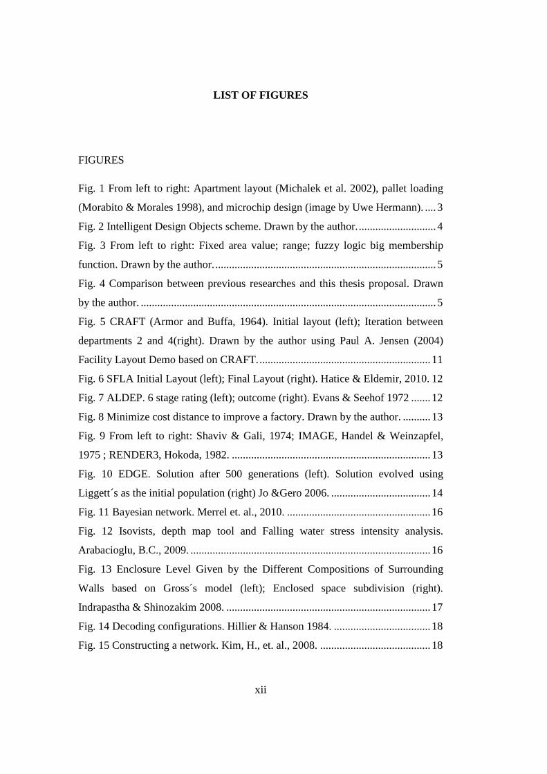
Fig. 1 From left to right: Apartment layout (Michalek et al. 2002), pallet loading

(Morabito & Morales 1998), and microchip design (image by Uwe Hermann). .... 3

Fig. 2 Intelligent Design Objects scheme. Drawn by the author. ............................ 4

Fig. 3 From left to right: Fixed area value; range; fuzzy logic big membership

function. Drawn by the author. ................................................................................ 5

Fig. 4 Comparison between previous researches and this thesis proposal. Drawn

by the author. ........................................................................................................... 5

Fig. 5 CRAFT (Armor and Buffa, 1964). Initial layout (left); Iteration between

departments 2 and 4(right). Drawn by the author using Paul A. Jensen (2004)

Facility Layout Demo based on CRAFT. .............................................................. 11

Fig. 6 SFLA Initial Layout (left); Final Layout (right). Hatice & Eldemir, 2010. 12

Fig. 7 ALDEP. 6 stage rating (left); outcome (right). Evans & Seehof 1972 ....... 12

Fig. 8 Minimize cost distance to improve a factory. Drawn by the author. .......... 13

Fig. 9 From left to right: Shaviv & Gali, 1974; IMAGE, Handel & Weinzapfel,

1975 ; RENDER3, Hokoda, 1982. ........................................................................ 13

Fig. 10 EDGE. Solution after 500 generations (left). Solution evolved using

Liggett´s as the initial population (right) Jo &Gero 2006. .................................... 14

Fig. 11 Bayesian network. Merrel et. al., 2010. .................................................... 16

Fig. 12 Isovists, depth map tool and Falling water stress intensity analysis.

Arabacioglu, B.C., 2009. ....................................................................................... 16

Fig. 13 Enclosure Level Given by the Different Compositions of Surrounding

Walls based on Gross´s model (left); Enclosed space subdivision (right).

Indrapastha & Shinozakim 2008. .......................................................................... 17

Fig. 14 Decoding configurations. Hillier & Hanson 1984. ................................... 18

Fig. 15 Constructing a network. Kim, H., et. al., 2008. ........................................ 18

xiii

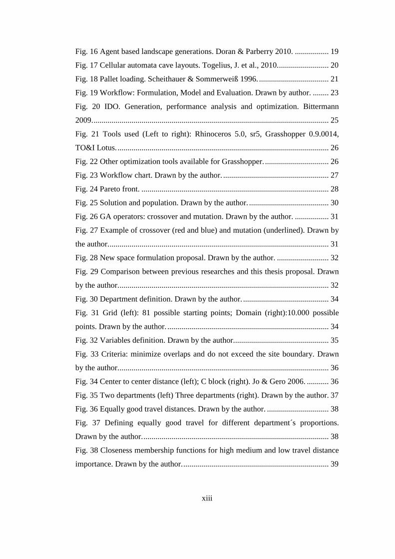
Fig. 16 Agent based landscape generations. Doran & Parberry 2010. ................. 19

Fig. 17 Cellular automata cave layouts. Togelius, J. et al., 2010. ......................... 20

Fig. 18 Pallet loading. Scheithauer & Sommerweiß 1996. ................................... 21

Fig. 19 Workflow: Formulation, Model and Evaluation. Drawn by author. ........ 23

Fig. 20 IDO. Generation, performance analysis and optimization. Bittermann

2009. ...................................................................................................................... 25

Fig. 21 Tools used (Left to right): Rhinoceros 5.0, sr5, Grasshopper 0.9.0014,

TO&I Lotus. .......................................................................................................... 26

Fig. 22 Other optimization tools available for Grasshopper. ................................ 26

Fig. 23 Workflow chart. Drawn by the author. ..................................................... 27

Fig. 24 Pareto front. .............................................................................................. 28

Fig. 25 Solution and population. Drawn by the author. ........................................ 30

Fig. 26 GA operators: crossover and mutation. Drawn by the author. ................. 31

Fig. 27 Example of crossover (red and blue) and mutation (underlined). Drawn by

the author. .............................................................................................................. 31

Fig. 28 New space formulation proposal. Drawn by the author. .......................... 32

Fig. 29 Comparison between previous researches and this thesis proposal. Drawn

by the author. ......................................................................................................... 32

Fig. 30 Department definition. Drawn by the author. ........................................... 34

Fig. 31 Grid (left): 81 possible starting points; Domain (right):10.000 possible

points. Drawn by the author. ................................................................................. 34

Fig. 32 Variables definition. Drawn by the author................................................ 35

Fig. 33 Criteria: minimize overlaps and do not exceed the site boundary. Drawn

by the author. ......................................................................................................... 36

Fig. 34 Center to center distance (left); C block (right). Jo & Gero 2006. ........... 36

Fig. 35 Two departments (left) Three departments (right). Drawn by the author. 37

Fig. 36 Equally good travel distances. Drawn by the author. ............................... 38

Fig. 37 Defining equally good travel for different department´s proportions.

Drawn by the author. ............................................................................................. 38

Fig. 38 Closeness membership functions for high medium and low travel distance

importance. Drawn by the author. ......................................................................... 39

xiv

Fig. 39 Neural tree structure. Drawn by author. .................................................... 40

Fig. 40 Fuzzy neural tree and fuzzy logic operations. Bittermann 2009. .............. 40

Fig. 41 Travel distance neural tree. Drawn by the author. .................................... 41

Fig. 42 Group neighborhood goodness neural tree definition. Drawn by Erald

Varaku and the author............................................................................................ 43

Fig. 43 Value input for public transport node. Drawn by the author. ................... 44

Fig. 44 Accessibility node weight values. Drawn by the author. .......................... 44

Fig. 45 Good neighborhood value outcome. Drawn by the author. ...................... 45

Fig. 46 Sensitivity analysis. Drawn by the author. ................................................ 46

Fig. 47 Sensitivity of three nodes. Drawn by the author. ...................................... 47

Fig. 48 Architectural decisions by parameter definition. Drawn by author. ......... 48

Fig. 49 Alignment by parameter definition. Drawn by author. ............................. 49

Fig. 50 Irregular site formulation. Drawn by author. ............................................ 49

Fig. 51 Custom value range for starting position for each element. Drawn by the

author. .................................................................................................................... 50

Fig. 52 Step-wise department assignment. Drawn by the author. ......................... 51

Fig. 53 Recursive subdivision of a rectangle in smaller rectangles. Drawn by the

author. .................................................................................................................... 52

Fig. 54 Polygonal subdivision. Doulgerakis 2007. ................................................ 52

Fig. 55 Variables and criterion summary. Drawn by the author. .......................... 53

Fig. 56 Case study 2: Bounding box. Drawn by the author. ................................. 55

Fig. 57 Case study 1: 6 departments; minimize overlaps. Drawn by the author. .. 57

Fig. 58 Case study 1: 6 departments; minimize overlaps and intersection with

boundary. Drawn by the author. ............................................................................ 57

Fig. 59 Case study 1: 6 departments; minimize overlaps, intersection with

boundary and bounding box area. Drawn by the author........................................ 57

Fig. 60 Case study 1: 6 departments; overlaps, boundary and travel distance after

100 generations, 150 population size. Drawn by the author. ................................ 58

Fig. 61 Case study 1: Minimize overlaps. Drawn by author. ................................ 58

Fig. 62 Case study 1: Region union. Drawn by the author. ................................... 59

xv

Fig. 63 Case study 1: Using solids to compute intersection. Drawn by the author.

............................................................................................................................... 59

Fig. 64 Case study 1: Solution sample for 6 departments using solids. Drawn by

the author. .............................................................................................................. 60

Fig. 65 Case study 1: 9 departments. Pareto front. Obtained by the author with

TO&I Lotus. .......................................................................................................... 60

Fig. 66 Case study 1: Solution sample after 442 generations, 50 population size.


Fig. 67 Case study 1: Solution sample after 105 generations, 150 population size.


Fig. 68 Constructive placement in grid network. Drawn by the author. ............... 61

Fig. 69 Allocation of six departments in a square grid of 1m cell. Drawn by the

author..................................................................................................................... 62

Fig. 70 Constructive placement. 8 departments of 60 m2. Drawn by the author. . 62

Fig. 71 Recursive divisions of a rectangle with three points resulting in 10

subdivisions. Drawn by the author. ....................................................................... 62

Fig. 72 Case study 2, site. American embassy in The Hague by M. Breuer. Photo

by Pvt Pauline. ...................................................................................................... 63

Fig. 73 Site plan. Drawn by the author. ................................................................ 64

Fig. 74 Case study 2: Site definition as a two dimension domain. Drawn by the

author..................................................................................................................... 65

Fig. 75 Case study 2: variables definition. Drawn by the author. ......................... 65

Fig. 76 Case study 2. Variable domain constraint to avoid street facades and

boundary intersection. Drawn by the author. ........................................................ 66

Fig. 77 Case study2. Summary of departments variables. p1,p2: position in axis 1

and 2. sf: starting floor. d1: axis 1 dimension. a: area. f: floor height (1 or 2

floors). ch: ceiling height. Drawn by author. ........................................................ 66

Fig. 78 Case study 2.Two goals. 150 population, 200 generations. Drawn by the

author..................................................................................................................... 67

Fig. 79 Case study2. Three goals. 200 population, 20 generations. Drawn by the

author..................................................................................................................... 68

xvi

Fig. 80 Case study 2. Incorporation of voids to the design. Drawn by the author. 68

Fig. 81 Case Study 2. Four goals Pareto front after 400 generations. Drawn by the

author. .................................................................................................................... 69

Fig. 82 Region included in region is not computed as intersection in Grasshopper.


Fig. 83 Case study 2. Mesh calculation flaw in Grasshopper. Drawn by the author.

............................................................................................................................... 70

Fig. 84 Solution outcome example. Drawn by the author. .................................... 70

1

CHAPTER 1

INTRODUCTION

In this thesis the spatial allocation problem is considered as a multi-optimization

problem. The model used is the Intelligent Design Objects. It is proposed as a

design tool and not as an automatization of the task. By studying and defining the

formulation of the problem and visualizing some result, the designer can adapt it

to his/her specific scenario and, gradually, build up the program relations.

The first chapter is an introduction to the spatial allocation problem. The second

chapter exposes a perspective of previous approaches to the matter as well as their

implementation in other industries, such as microchip and gaming industries.

The model used is explained in the third chapter: the tools used, the workflow and

the use of optimization and genetic algorithms. Chapter four describes the

mathematical formulation: the parameter definition, criterion definition and the

implementation of fuzzy logic. The fifth chapter includes examples to evaluate the

results and concludes with the application to a case study: the graduation project

at TUDelft.

Finally, conclusions about the research and suggestions for further studies are

presented.

2

A building layout plan is the representation of the configuration and arrangement

of different spatial elements in a building. Topological relations as alignment and

adjacency; geometric properties such as shape, dimension and rotation are the

main concerns in spatial synthesis (Eastman, 1973). It is one of the most difficult

problems in architectural design as it has a significant impact on their function and

accessibility.

A common workflow in architectural practice begins with refining the client´s

requirements into an architectural program with diagrammatic representation of

the rooms and connections (concept design process). In a later stage the program

is used to generate floor plans. During this process, the architect reformulates the

program as the importance of new relations are revealed, or the number of rooms

redefined. The architect/s would study some of the outcomes and chose or propose

to the client which one is the best. Due to the high number of possible

combinations, the use of computers is advised for this operation. The task stands

as an optimization problem, understood as the procedure or procedures used to

make a system or design as effective or functional as possible.

As an example, for a family house building layout, the rooms are the elements to

be arranged; the sizes and positions of each of them are parameters that will

generate different solutions. Each outcome solution has different properties

(dimensions, proportions, orientation, etc.) and there has to be some criteria and/or

goals to compare them to be able to decide which one is better. Crisp goals

(clearly measurable) are defined such as adjacencies, distances, total area, solar

gain, etc. Fuzzy logic is introduced to address other concepts that are difficult to

measure. For example, the concept of “big room”. This is referred as fuzzy

because the exact value when a room is or is not considered “big” is not clear, it is

subjective to the user. The implementation of these fuzzy concepts into the spatial

allocation problem brings more design freedom in opposite to most of the

previous researches on the topic whose formulations limit it.

It is likely that some of the goals introduced are conflicting and, as the value of

one grows, the value of the other decreases. In the example, the bigger solar gain

3

would come if the rooms are separated and a larger surface perimeter is presented

to receive the sun but, at the same time, it results in larger walking distances

among the rooms, ending up in a non-functional solution. Therefore, the search

aims for a solution where all the objectives are in some degree satisfied.

Many researches have addressed the spatial allocation problem for building

layouts and for other industries. However, their application is usually limited by

the rigidity of their formulations. Some limit themselves to a certain type of

building (residential), and their results cannot be extrapolated to other types.

Others introduce the cost function of the overall solution and aim to minimize it.

This is desirable in certain scenarios, but does not satisfy other architectural

needs. The desired program relations in architecture are not a priori known, and

are also different from project to project. Therefore the application of these

researches in the field of Architecture has been limited, while micro-chip industry

or pallet loading have successfully implemented them.

Fig. 1 From left to right: Apartment layout (Michalek et al. 2002), pallet loading (Morabito & Morales 1998), and microchip design (image by Uwe Hermann).

In this thesis the aim is to approach the spatial allocation problem through

performance based design. The use of the cost function to compare different

solutions is very limited. Instead, the user is intended to define the criteria for

A

A

AA

A

A

Bath

Hall

Hall

Kitchen

Bedroom

Bedroom

DinningRoom

LivingRoom

Pallet loading Microchip designApartment layout

4

every specific scenario. Besides, the desired relations among the departments is

not known and it is a process subject to changes. Questioning and formulating

these relations is an important part of the design process. While previous methods

take for granted that the relations are known, in this research it is part of the

department parameter definition. As such, it is meant to be adapted and refined

throughout the design process. Therefore, it is needed a tool that allows user

customization.

The method adopted is called Intelligent Design Objects (IDO). IDO (Bittermann

2009) consists in generation of possible solutions, their evaluation regarding

previously defined criteria, and generation of new solutions that improve the

previous solutions (with the use of genetic algorithms).

Fig. 2 Intelligent Design Objects scheme. Drawn by the author.

Multiple criteria instead a single criterion enables enhanced architectural

outcomes. Likewise, both crisp and fuzzy goals are included as part of this multi-

objective optimization. The use of fuzzy goals or objectives is included to echo

the process taken in architectural design, especially in the early stage, but is not

exclusive to this field. In the case of previous methods, each department area is

fixed to a certain value, in most cases, or to a range of values. Fuzzy logic is

included to extend the exploration of more solutions. For example, in a residential

project the living room is desired to be “big”. With other methods, the area value

would be fix to 25 sq. m. or to a range of values from 20 to 30 sq. m. This

excludes the consideration of solutions in which the living room is larger or

GENERATESOLUTIONS

COMPARESOLUTIONS

OPTIMIZESOLUTIONS

5

smaller and, as such, it is a limitation. On the contrary, defining the abstract

concept of “big” as a function allows a much wider solution exploration.

Fig. 3 From left to right: Fixed area value; range; fuzzy logic big membership function. Drawn by the author.

Defining this function is also part of the project analysis and reflects the designer

intentions in a clear way and/or addresses the client wishes.

Fig. 4 Comparison between previous researches and this thesis proposal. Drawn by the author.

The increased freedom is reflected in an increase of the number of possible

solutions. In order to deal with this high number of solutions a heuristic strategy is

used, such as evolutionary algorithms. The encyclopedia Britannica defines

heuristic “as relating to exploratory problem-solving techniques that utilize self-

educating techniques (as the evaluation of feedback) to improve performance”.

Also notice that the outcome with such method is not guaranteed to be optimal

25 sqm 20sqm

0 2010 30 40 50 area (sq. m.)

big

me

mbe

rsh

ip d

egr

ee

130sqm

PREVIOUS

Limited design freedom(grid, building type)

Single objective

Closed toolAutomatization tool

Crisp objective

PROPOSED

Increased design freedom(user/project defined)

Multiple objectives

Crisp and Fuzzy objectives

Open tool, customizableDesign tool

6

but, since it is unfeasible to analyze every possible solution, the aim is to find

satisfactory solutions for the problem.

Within the scope of this thesis some examples will be studied and the graduation

project for TUDelft will be used as a case for the evaluation of the model. This

model, IDO, is suitable to be used for different building types and/or different

problems than the spatial allocation, while the problem formulation and the

criteria are user defined for each particular scenario.

7

CHAPTER 2

LITERATURE REVIEW

The use of a tool, any tool, in the design process seeks to enhance the quality of

the design. In the case of computer tools, productivity, efficiency, precision, etc.,

but are not admissible if they restrain design freedom. Many studies have been

carried out about the spatial allocation problem, and applied successfully in some

fields, such as microchip industry. The microchip industry strived for a solution

for chip layout design that minimize wiring costs, and researches like Khokhani &

Patel (1977) were implemented effectively.

In many cases, researchers evaluated their software with architectural exercises.

Liggett´s (1980) application to a hospital department organization, and coming

studies seemed to open the path to practitioners. However, the limited design

freedom (based in cellular module grid, for example), and/or the difficulty of the

implementation (complex travel cost matrixes) have kept architects away from

using these methods.

In the coming chapter, a review of previous researches is presented.

8

9

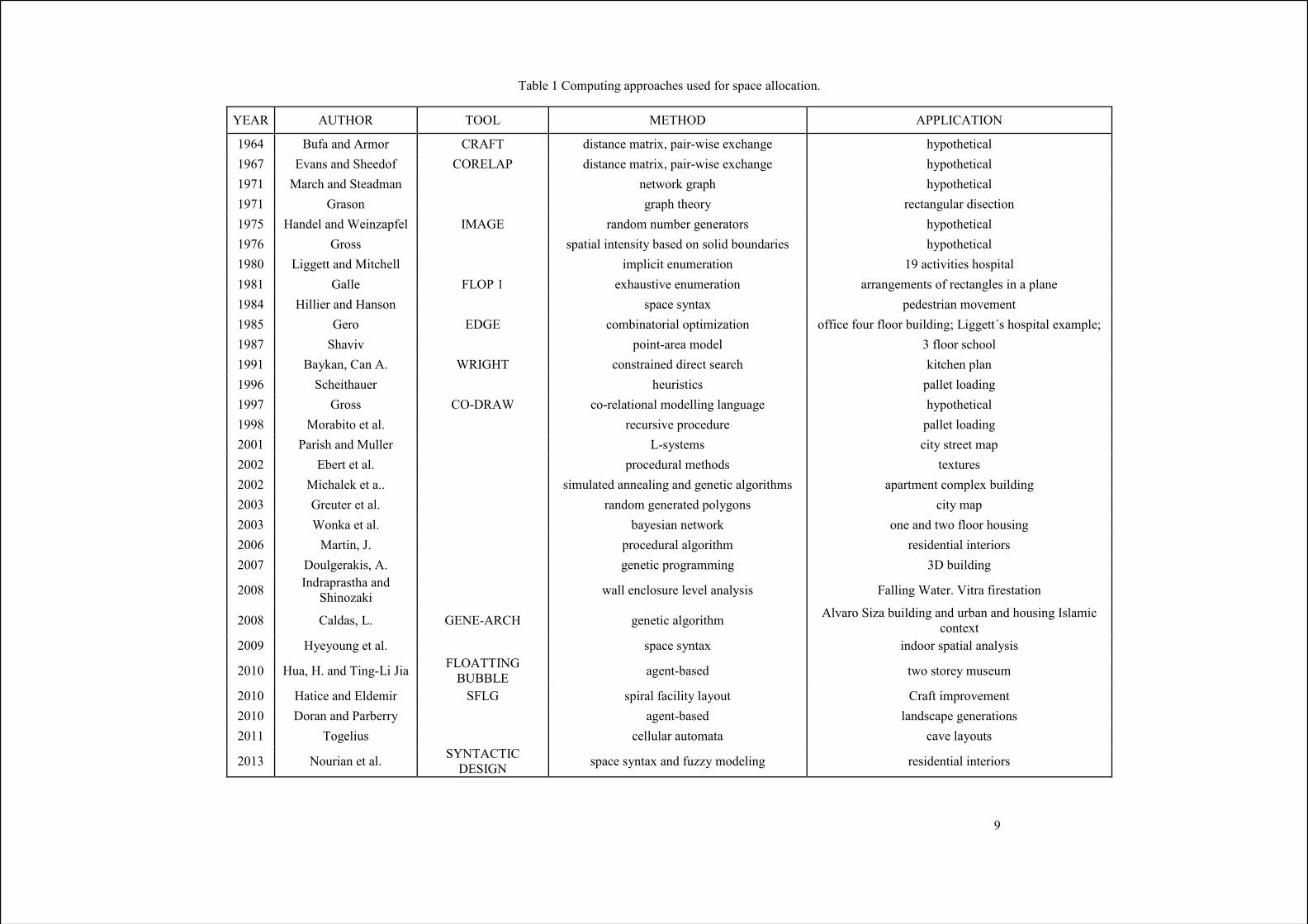
Table 1 Computing approaches used for space allocation.

YEAR NOITACILPPA DOHTEM LOOT ROHTUA

itehtopyh egnahcxe esiw-riap ,xirtam ecnatsid TFARC romrA dna afuB 4691 cal ehtopyh egnahcxe esiw-riap ,xirtam ecnatsid PALEROC fodeehS dna snavE 7691 tical

1971 March and Steadman lacitehtopyh hparg krowten1971 Grason noitcesid ralugnatcer yroeht hparg

lacitehtopyh srotareneg rebmun modnar EGAMI lefpaznieW dna lednaH 57911976 Gross lacitehtopyh seiradnuob dilos no desab ytisnetni laitaps1980 Liggett and Mitchell latipsoh seitivitca 91 noitaremune ticilpmi1981 Galle FLOP 1 exhaustive enumeration arrangements of rectangles in a plane 1984 Hillier and Hanson tnemevom nairtsedep xatnys ecaps1985 Gero EDGE combinatorial optimization office four floor building; Liggett´s hospital example; 1987 Shaviv loohcs roolf 3 ledom aera-tniop

nalp nehctik hcraes tcerid deniartsnoc THGIRW .A naC ,nakyaB 19911996 Scheithauer heuristics pallet loading

lacitehtopyh egaugnal gnilledom lanoitaler-oc WARD-OC ssorG 79911998 Morabito et al. gnidaol tellap erudecorp evisrucer2001 Parish and Muller pam teerts ytic smetsys-L2002 Ebert et al. serutxet sdohtem larudecorp2002 Michalek et a.. simulated annealing and genetic algorithms apartment complex building 2003 Greuter et al. pam ytic snogylop detareneg modnar2003 Wonka et al. gnisuoh roolf owt dna eno krowten naiseyab2006 Martin, J. sroiretni laitnediser mhtirogla larudecorp2007 Doulgerakis, A. gnidliub D3 gnimmargorp citeneg

2008 Indraprastha and Shinozaki wall enclosure level analysis Falling Water. Vitra firestation

2008 Caldas, L. GENE-ARCH genetic algorithm Alvaro Siza building and urban and housing Islamic context

2009 Hyeyoung et al. sisylana laitaps roodni xatnys ecaps

2010 Hua, H. and Ting-Li Jia FLOATTING BUBBLE muesum yerots owt desab-tnega

tnemevorpmi tfarC tuoyal ytilicaf larips GLFS rimedlE dna ecitaH 01022010 Doran and Parberry snoitareneg epacsdnal desab-tnega2011 Togelius stuoyal evac atamotua ralullec

2013 Nourian et al. SYNTACTIC DESIGN sroiretni laitnediser gniledom yzzuf dna xatnys ecaps

10

11

2.1 Literature

The assignment of architectural discrete space elements in the plane to their

locations is known as the spatial allocation problem. The relationships between

the space elements include topology and geometry. Determining these relations

make the design process complicated due to its combinatory nature. The use of

computers was instated for automating this task. Automated spatial allocation

aimed to assist architects during the conceptual design process. Since 1960 many

soft tools have been developed for finding automated solutions for this problem.

The first attempts focused on producing arrangements of rectangles in a plane, or

on the allocation of grid cells. Armor and Buffa were the first in 1964 to formulate

the layout problem as a quadratic assignment problem. They considered the cost

between departments to be the criterion to minimize. For that, they developed

Computerized Relative Allocation of Facilities Technique (CRAFT). Probably

their work was influenced by Eldars and Whitehead´s study, on the same year, on

the pedestrian movement in a hospital (which turned to be 23%).

Fig. 5 CRAFT (Armor and Buffa, 1964). Initial layout (left); Iteration between departments 2 and 4(right). Drawn by the author using Paul A. Jensen (2004) Facility Layout Demo based on

CRAFT.

The limits of the CRAFT were extended (Hatice & Eldemir 2010) SFLA, or

Spiral Facility Layout Generation and Improvement Algorithm. The aim is to

gather the most frequently used spaces at the center, as it will minimize the

distance between them.

2222 2

22222

444444 4 4 4 41

1111

3 3 3 3 3333333333333333

6 6 6 6 666666

4 4 4 44444

444444444444

7 7 7 7 7

5 5 5 5 55555555555

55555

9 9 9 9 9999999999999999

8 10 10 101010108101010810101081010108101010810101081010108101010810101088 10 10 10

8 10 10 108 10 10 108 10 10 108 10 10 108 10 10 108 10 10 108 10 10 108 10 10 10

1010108

9 9 9 9 99 9 9 9 99 9 9 9 9

99999

5 5 5 5 5

5 5 5 5 55 5 5 5 5

55555

777774 4 4 4 44 4 4 4 44 4 4 4 44 4 4 4 44 4 4 4 4

44444

6 6 6 6 666666

3 3 3 3 33 3 3 3 33 3 3 3 3

333332 2 2 2 2

22222

11111

12

Later, Lee & Moore (1967) and Evans and Seehof (1972) developed

Computerized Relationship Layout Planning (CORELAP) and Automated Layout

Design Program (ALDEP) respectively, based on the importance of a set of

pairwise evaluations of the closeness of two activities, rating them in 6 stages:

Absolute essential, essential, important, ordinary, unimportant and undesirable.

Fig. 6 SFLA Initial Layout (left); Final Layout (right). Hatice & Eldemir, 2010.

Fig. 7 ALDEP. 6 stage rating (left); outcome (right). Evans & Seehof 1972

These algorithms focus on the transportation cost function as the combination of

flow, distance and unit cost. It is useful for organizing a production factory,

defining the machinery tools as the departments, the moving cost and the flow

chart. Its limitation is that it assumes that move costs are linearly related to the

length of the move and that are independent of the department.

2

2E

U

EO I

I

AU

IO

UO

I

U

U UU

UU

E

U

A= Absolutely Essential E= Essential I= I mportantO= Ordinary U= Unimportant X= Undisirable

21

1

3

33

4 45

5

6 67 7ALDEP RELATIONS CHART TOTAL CLOSENESS RATING = 228

13

Fig. 8 Minimize cost distance to improve a factory. Drawn by the author.

Handel and Weinzapfel (1975) developed a three dimensional layout planning

named IMAGE, in which a set of rectangular volumes represented the building

functions. These volumes are defined by a set of dimension, position, and rotation.

A set of constraints such as alignment, proximity and circulation form the

constraints and the objective is to satisfy all of them.

Approaches that attempt to enumerate all possible arrangements with a specified

number of rooms (Galle 1981), face the problem that increasing the number of

elements (rooms) grows the possible arrangements exponentially, making this

approach very limited. Others attempted to find “a good” arrangement using

greedy local search over possible partitions of a regular grid (Shaviv & Gali

1986).

Fig. 9 From left to right: Shaviv & Gali, 1974; IMAGE, Handel & Weinzapfel, 1975 ; RENDER3, Hokoda, 1982.

Other studies continued investigating the spatial allocation problem, such as

Liggett (1980), Hokoda (1982), Akin (1992), Yoon and Coyne (1992). It is seen

that three major issues common to all of them arose:

sto

rage

Ass

embl

y

Sho

p

Lathe Drill DrillGrind

Drill

DrillPress Bend

Mill

14

The complexity of the problem (due to its non-linearity).

How to control the possible combinations.

How to evaluate the solutions.

The first one is inherent of the problem. It is referred as non-linear because the

output is not directly proportional to the input.

Different algorithms deal with the control and evaluation of this problem in

different ways. Liggett assigns the size of the space elements to modules. The

assignment strategy is the multi-stage that includes floor, zone and block to locate

the modules, and the largest spaces are placed first.

Jo & Gero 1985 implemented in C language the Evolutionary Design based on

Genetic Evolution system (EDGE). They evaluated its performance by solving the

same space layout attempted by Liggett in 1985.

Fig. 10 EDGE. Solution after 500 generations (left). Solution evolved using Liggett´s as the initial population (right) Jo &Gero 2006.

It considers a set of 21 office departments to be placed in a building with 4 floors,

divided into 17 zones. Their results indicate their strategy is less dependent on the

initial population than Liggett´s and finds solutions closer to the global optimum.

EXEC 0240 0240

access access access access

0500

0500

021002100211

0220

0220

0230 0230

0211

0300

0300

0700

0700

0700

0700

0400

0400

0900

0900 0900

0900

6300

6300

6815

6815

0600 0600 6881

1000

1000 1000

1000

6881

0800

EXEC

15

Other strategies are constructive placement and pair-wise improvement. Graves &

Whinston (1970) developed the constructive placement. It is a strategy of n-stage

decision process, and locates activities one by one starting with an empty set. The

next element is chosen based on the objective function. Then pair-wise change is

used. It evaluates possible changes between pairs of activities and makes the

exchange if it improves the value of the criterion for the highest value. The

solution obtained is very dependent on the initial solution.

The change is applied on pairs of neighboring units, and not possible on units over

3 or more even it may produce a better solution. For example if the units consist

of “0 1 1 0” and the objective is to locate the same kind of units together, the

solution may never get “0 0 1 1” or “1 1 0 0” because it will not accept any

change that would make the performance decrease immediately compared to the

previous state. This is a limitation of the pair-wise method to find an optimal

solution because even a decrease in performance in one pair exchange could lead

to an improvement by the next exchange.

Recent studies have pointed out the suitability of data driven approach. Following

Koller and Friedman (2009) probabilistic models, P. Merrell, E. Schkufka and V.

Koltun (2010) structured relationships among features in architectural programs.

They used Bayesian network to represent probability distribution over the space.

For example, a kitchen is more likely to be adjacent to a living room than to a

bedroom; three bedrooms increase the need of a second bathroom. These relations

are often implicit in architect´s expertise but not clearly represented with ad-hoc

optimization approaches. In Merrell et al., they encoded 120 architectural

programs of residential layouts to train the Bayesian network. Their data is highly

structured based on global (total area and footprint) and per room basis.

To convert the graph into a building layout, the metropolis algorithm is used.

Metropolis-Hasting algorithm is a Markov chain Monte Carlo to obtain a

randomly distribution when direct sample is difficult. As Sullivan & Beichl state

(2000, p.69) “Monte Carlo is a last resort, to be used only when no exact analytic

method or even finite numerical algorithm is available”.

16

Very large scale integration layouts (VSLI) and their trained Bayesian network

took an average of 35 seconds to generate a layout. But many factors were not

taken into account (such as climate, views, site, client desires, curved spaces…).

Fig. 11 Bayesian network. Merrel et. al., 2010.

2.2 Selection criteria

To evaluate the performance of each solution for privacy-publicity or inclusivity-

exclusivity analysis Arabacioglu (2009) uses fuzzy inference and isovists. It is an

attempt to quantify architectural space, since the distance objects and visibility

provides different experience.

Fig. 12 Isovists, depth map tool and Falling water stress intensity analysis. Arabacioglu, B.C., 2009.

Feature Domain

Total Square Footage ZFootprint Z × ZRoom {bed, bath, . . . }Per-room Area ZPer-room Aspect Ratio Z × ZRoom to Room Adjacency {true, false }Room to Room Adjacency Type {open-wall, door }

LivingRoom-

KitchenAdjacency

Type

TotalSquareFootage

Footprint

LivingRoomExists

KitchenExists

KitchenArea

LivingRoom-Kitchen

AdjacencyExists

LivingRoomArea

KitchenAspectRatio

LivingRoomAspectRatio

17

Indraprastha & Shinozakim (2008) study the experience of an architectural space

as a product of out movement and perception, or as a result from the arrangement

of its boundary elements. They refer to Gross (1997) and measure the level of

spatial intensity based on number of solid boundaries. According to them each

enclosed space is classified by the number of adjacent walls.

Their study consists in calculating enclosed spaces and axial lines to establish the

enclosed spaces relative to a circulation space, and the determination of

subdivided enclosed spaces using territorial lines. The main limitation of their

model is to try to measure spatial intensity as a human experience but leaving the

material properties like texture of opacity out of the model.

Fig. 13 Enclosure Level Given by the Different Compositions of Surrounding Walls based on Gross´s model (left); Enclosed space subdivision (right). Indrapastha & Shinozakim 2008.

Accessibility has been applied to urban problems. For large buildings, the

interspatial accessibility among the parts is taken into account for evacuation

planning, for example. Accessibility refers to the relative nearness from one place

to another. It has been used mainly in 2D for urban cases but, in a building, those

relations are 3D. Space syntax has been used to study the connectivity of

architectural spaces. It has been applied in the attempt to model pedestrian

movements to compute the network connectivity of the built environment.

0/412

2

2

2 2

2 2

2

2

23

3

3

3

33

1

1 1 11 1

11

1 11

1/4

2/4

2/4

3/4

4/4

18

Fig. 14 Decoding configurations. Hillier & Hanson 1984.

Hyeyoung Kim, Chuilmin Jun, Yongjoo Cho and Geunhan Kim (2008) already

reflect the main drawback of this approach: the difficulty of computing the costs

taken in movement among spaces, like turns or floor transfers. They used the

shortest path algorithm by Dijkstra, 1959, composed of node selection operation

and distance update but they conclude that the depth of the linear space is not

applicable to indoor spaces so they added penalties for turns and movement

between floors (and called it “impedance”).

Fig. 15 Constructing a network. Kim, H., et. al., 2008.

Recent studies (Doulgerakis 2007), propose genetic programming (GP) instead

genetic algorithms. The restriction of GAs is their fixed genotype length. GP is

based on the idea that the structure of the attributes and their magnitude for the

optimal solution are part of the answer and not on the question. Doulgerakis

considers the layout problem as a program induction problem. The genotypes are

expressed as tree-like recursive structures. The end nodes are spaces with two

variables (width and height) and the intermediate nodes are transformation

operations (move forward, rotate ad scale). That strategy, as he noted, led to a

a a= =b a ab b

b

c

cc

c

19

confusing process where separation and overlapping was difficult to avoid, and

more inefficient when the outline of the site is given.

2.3 Other applications of the spatial allocation problem.

Microchip industry has successfully used iterative algorithms in their designs.

Khokhani & Patel (1977) presented the benefits on the chip layout problem. The

constructive methods obtain the initial solutions and the wirability evaluation and

the wire length are used as constraint and criterion, respectively.

Maps generation is another interesting approach. Useful for creating terrains, the

particle deposition algorithm drops particles at random locations. These particles

move down till they reach other particle or the ground. Heights are adjusted or

randomly determined. Same approach could be used for a layout configuration,

although it may need other rules to bring significant architectural results.

Using multiple software agents (Doran & Parberry 2010) implement five agents

with specific tasks to generate a landscape. The way they conceive their agents to

create flat areas, mountains of paths could also be helpful when searching for a 3D

building layout. But, for now, these approaches are more used by gaming

industries than architecture firms due to the difficulty of the evaluation of the

results.

Fig. 16 Agent based landscape generations. Doran & Parberry 2010.

20

An algorithm with low computational cost allowing real time generations:

cellular automaton. It is a collection of cells on a grid that evolves with a set of

rules based on the neighboring cells. It has been used by Stanle, Yannakakis &

Togelius (2010), to generate cave or dungeon layouts. After it runs the cave is

evaluated to determine it if is acceptable or not. If some of the cells do not connect

to the initial grid, the closest two are joined by a tunnel. At last, inconsistencies

are removed or smoothing is performed.

Fig. 17 Cellular automata cave layouts. Togelius, J. et al., 2010.

The increase in video games realism, has led to better real time buildings

generations. Togelius et al., generate complete maps using a search-based

procedural content generation (SBPCG). This algorithm does not only accept or

reject a candidate: it grades the solution by assigning a numerical value.

The Rectangle Pallet loading consists in finding a pattern to pack small rectangles

in a larger rectangle, so that the area used is maximized (Scheithauer &

Sommerweiß 1996). Pieces of different height are combined, resulting in a three

dimensional problem.

21

Fig. 18 Pallet loading. Scheithauer & Sommerweiß 1996.

As it is exemplified, spatial allocation problem has been applied successfully in

many fields such as microchip manufacturing, pallet loading or factory tool

disposition. Architectural problem solving, understood as the search and selection

of solution alternatives during sketch design phase, still remains more to

researchers than to practitioners (Galle 1981). The compromise in formulations

needed to overcome the difficulty of the problem, in computation costs, result in

many tools that claim partial good results but lack of design freedom. Some

constrain themselves to grids (Armor & Buffa, Liggett & Mitchell, Gero, etc.)

others to specific architectural types (Wonka et al.) and, in general, the

departments are set as modules or rectangles. The difficulty of the architectural

problem relies both on defining the relations and on the goal definition. The

architect does not know a priori what are the relations among the departments

neither what is the importance of every goal. Maximizing the used area (as in

pallet loading) is certainly an architectural objective, but it is not the only one. In

fact, the complexity of architectural design requires the consideration of multiple

objectives.

In this thesis, since the relations are not defined, the computer is used as a design

tool and not as an automated tool. The emphasis is put on the search of a basic

layout that will be later modified and refined into a building layout. The use of

rectangular shape pursues a reduction of computational costs, since it is up to the

user modifying the solution into irregular shapes to his/her will. The computer

produces some initial solutions in relation with the first set of inputs, and new

22

relations come to the designer’s mind, who redefines the inputs and runs the

process again till a satisfying solution is found. In constructive approaches, the

departments are added one by one, in relation to the previous state. In this thesis

an iterative approach is pursued as the relations are not a priori established. By

visualizing new solutions, new relations and/or their relative importance come

out. However, to assure design freedom, the spatial allocation problem has to be

formulated in a flexible manner, able to respond to different project scenarios.

This is explained in the upcoming chapters.

23

CHAPTER 3

MODEL

In the previous chapter an overview of previous researches was presented. Their

formulations, in most of them, differ and it is not possible to compare their results.

Some of them have been successfully applied in other fields, such as pallet

loading and microchip design, but the architecture scene is still reluctant to their

usefulness.

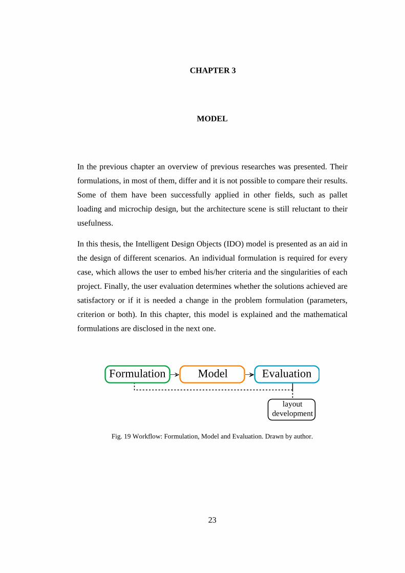
In this thesis, the Intelligent Design Objects (IDO) model is presented as an aid in

the design of different scenarios. An individual formulation is required for every

case, which allows the user to embed his/her criteria and the singularities of each

project. Finally, the user evaluation determines whether the solutions achieved are

satisfactory or if it is needed a change in the problem formulation (parameters,

criterion or both). In this chapter, this model is explained and the mathematical

formulations are disclosed in the next one.

Fig. 19 Workflow: Formulation, Model and Evaluation. Drawn by author.

Formulation Model Evaluation

layoutdevelopment

24

3.1 Approach

In this thesis the project is treated as a space allocation design problem. The

computer is used to help the designer to define the different relations among the

departments of the program proposed. Visual feedback is provided to guide the

designer. Since these relations are not a priori established, the author does not aim

to achieve the automatization of the task. Instead, a progressive refinement of

these parameters and relations is carried out. The custom based formulations

allow design freedom and flexibility to be applied to different projects. The

number of criteria affects critically to the computation required to find optimum

solutions. Once more, it is subject to the user the number of criterion to be

considered, and their relative importance.

As seen before, the three main issues are:

The complexity of the problem (due to its non-linearity).

How to control the possible combinations.

How to evaluate the solutions.

To cope with these three topics, the Intelligent Design Objects methods (IDO) is

used (Bittermann 2009). IDO consists of three steps: the first is the generation of

possible solutions. The second is performance analysis. A set of criteria is defined

to compare the outcome of the generations. Finally, an optimization process to

obtain better solutions, with the use of genetic algorithms is presented.

25

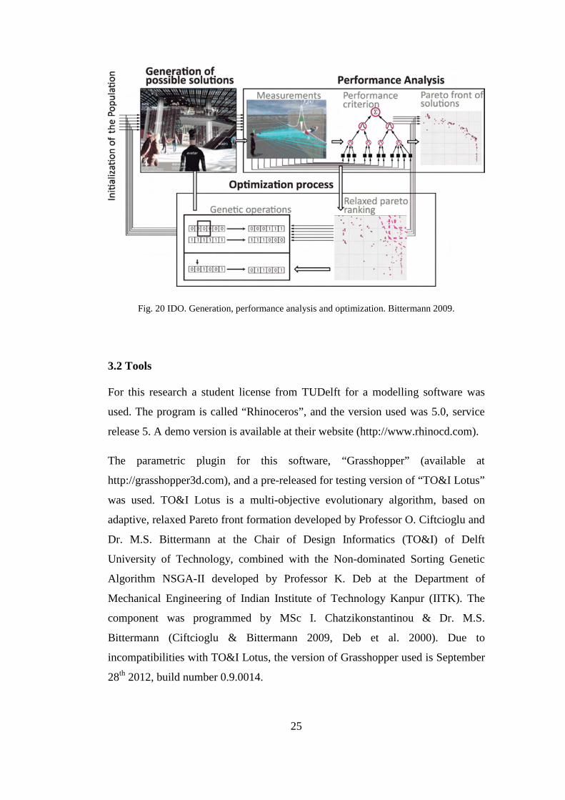
Fig. 20 IDO. Generation, performance analysis and optimization. Bittermann 2009.

3.2 Tools

For this research a student license from TUDelft for a modelling software was

used. The program is called “Rhinoceros”, and the version used was 5.0, service

release 5. A demo version is available at their website (http://www.rhinocd.com).

The parametric plugin for this software, “Grasshopper” (available at

http://grasshopper3d.com), and a pre-released for testing version of “TO&I Lotus”

was used. TO&I Lotus is a multi-objective evolutionary algorithm, based on

adaptive, relaxed Pareto front formation developed by Professor O. Ciftcioglu and

Dr. M.S. Bittermann at the Chair of Design Informatics (TO&I) of Delft

University of Technology, combined with the Non-dominated Sorting Genetic

Algorithm NSGA-II developed by Professor K. Deb at the Department of

Mechanical Engineering of Indian Institute of Technology Kanpur (IITK). The

component was programmed by MSc I. Chatzikonstantinou & Dr. M.S.

Bittermann (Ciftcioglu & Bittermann 2009, Deb et al. 2000). Due to

incompatibilities with TO&I Lotus, the version of Grasshopper used is September

28th 2012, build number 0.9.0014.

26

Fig. 21 Tools used (Left to right): Rhinoceros 5.0, sr5, Grasshopper 0.9.0014, TO&I Lotus.

The decision of a graphic interface over a programming language was to obtain

visual outcome and interaction with the user. In the scenarios that the plugin

performance was critical, other available plugins were tested: David Rutten’s

“Galapagos”; Simon Flöry’s “Goat 2.0”; and Vierlinger & Zimmel’s “Octopus

0.1”). Galapagos and Goat are single objective while Octopus is multi-objective.

However, the number of parameters that TO&I Lotus is able to cope with is, at the

moment this research was performed, much larger than in Octopus.

Fig. 22 Other optimization tools available for Grasshopper.

3.3 Workflow

In the following figure, three sets of actions are presented. The first one is referred

as “formulation” and it is user defined and specific for every particular project.

The second one is the model used, IDO. The last one is a personal evaluation of

the outcome that leads to a reformulation of the problem, or to the layout

development.

27

Fig. 23 Workflow chart. Drawn by the author.

These sets are performed in a loop sequence, because the relations and proportions

of the departments are not pre-defined, until a satisfactory solution is found. As

explained before, this method does not seek for the optimal solution (since the

number of possibilities is high), but to provide satisfactory ones.

3.4 Optimization

The spatial allocation problem is treated as an optimization problem in this thesis.

In particular, the selection of the best set of positions and dimensions for a group

of departments regarding the criteria defined. It is possible to combine these

criteria into a single objective (also called as cost function) by combining with

weights their relative importance, to minimize or maximize. The limitation of the

single objective approach is that it requires fixing the weights in the objective

SPACEDEFINITION

VARIABLEDEFINITION

CRITERIADEFINITION

GENERATESOLUTIONS

COMPARESOLUTIONS

OPTIMIZESOLUTIONS

EVALUATERESULTS

SATISFACTORY

DEVELOPLAYOUT

UNSATISFACTORY

IDO

2nd ordercriterion

1st ordercriterion

Formulation

Model

Evaluation

28

function, while before finding optimal solutions it is unknown what the trade-offs

are that characterize the problem.

For a multi-objective optimization problem, there is not a unique solution that

optimizes each objective at once. This is due to the conflicting nature of some

objectives. For example, in case that the smallest boundary that contains all the

elements is required and, at the same time, the intersection of the elements is to be

minimized. The smallest boundary optimum would intersect all of the elements,

so the goal is to search where both criteria are satisfied. Particularly, the purpose

is to search for non-dominated solutions. A solution is non-dominated if there is

no other solution that performs better in every aspect. If analyzed the performance

of a large number of design options in the objective function space for evaluation,

the outer boundary of this collection of points defines the borderline limit beyond

which the design cannot be further improved. When compared to any other

solution, a non-dominated solution is superior for at least one criterion. This is

referred as Pareto optimal solution. The group of Pareto optimal solutions is

called Pareto frontier, or Pareto front.

Fig. 24 Pareto front.

population

feasible solution

Pareto frontier

Utopian solution

Unfeasible solution

objective 1

objective 2

29

Without additional subjective preference information, all Pareto optimal solutions

are considered equally good. By using this method the solutions concerning

several goals are investigated without combining them beforehand.

3.5 Genetic algorithm

In the spatial allocation problem, the combination of possibilities is very high. It is

not feasible to investigate all of them. Approaches like Galle (1981), who

enumerated exhaustively all the possible solutions, are not useful.

For example, in a design with 10 departments, 4 variables each, and 10 possible

states the amount of combinations is 1040. Considering that a computer takes a

single cycle to process the performance of one of those combinations and that the

processor has a frequency of 10 GHz, it would take 1030 seconds to analyze all the

solutions, which is millions of years.

To deal with this high number of combinations the method used in this thesis is

the evolutionary search. It explores the possible solutions starting with a set of

random ones and next states are determined by probability distribution, belonging

to the stochastic methods. It relates to the combination of genetic material of

species. The genetic material of the resulting individual matches the best of the

parents or even outperforms it. This principle is used in evolutionary computation

and it is known as genetic algorithm (GA).

A set of candidate solutions is referred as population. In this research, a solution

consists of a set of positions and sizes of the departments. A population is a set of

solutions.

30

Fig. 25 Solution and population. Drawn by the author.

The first population is the outcome of random values of the parameters defined.

Solutions from the first population are taken to form a new population. This is

motivated by the aiming to improve features of the new population. The selection

is according to the fitness or suitability to provide more probability to reproduce.

This is determined by the performance of the solutions for the criteria defined.

According to their fitness, the chromosomes are given a chance to survive to the

next generation. This is called reproduction. Then it is repeated for a number of

populations or till a “best solution” is achieved. But in order to increase the

performance some operations are taken. In this thesis the operators of GA used are

crossover and mutation.

The solutions of a population are coded into binary strings, or chromosomes. The

first step is called selection which takes the fittest chromosomes. Crossover

selects genes from parents and creates a new child (called offspring). It chooses

randomly a point and copies the string before the point from the first parent and

everything after from the second. The objective of the crossover is to maintain

features of the parent solution and explore different places in the search space.

After mutation is performed mutation is done to prevent from local optimum

solutions. Mutation changes randomly a few bits from 0 to 1 or from 1 to 0.

overlaps

tota

l bo

und

ary

population

solution

31

Fig. 26 GA operators: crossover and mutation. Drawn by the author.

A layout solution is a set of departments. These departments are defined by the

starting point, area and the dimension of one of their sides. These values are coded

into a binary string. With the use of the crossover operator, part of that string will

be maintained in the next generation. In figure 27, the first two chromosomes are

combined to generate the third solution.

Fig. 27 Example of crossover (red and blue) and mutation (underlined). Drawn by the author.

For the author, the previous researches presented significant limitations that

prevent architects to take advantage of them. The first limitation is regarding the

number of criterion. Cost function optimization is useful in some fields, and it is

also beneficial in certain architectural cases, although it is not sufficient to express

the complexity of architectural design. Therefore, multiple objectives are

introduced, and a model (IDO) is presented to cope with the high amount of

possible solutions. Evolutionary search is used in the optimization process in

order to obtain satisfactory solutions since exhaustive search is not feasible.

Chromosome 1 11011 00100110110

11010 11000011110

11011 11000011110

11010 00100110110

Crossover Mutation

Chromosome 2

Offspring 1

Offspring 2

Original offspring 1 1101111000011110

Original offspring 2 1101100100110110

Mutated offspring 1 1100111000011110

Mutated offspring 2 1101101100110100

101011100101011100110 11101010111010101010 1010101001111010011010

32

Custom formulation grants design flexibility and user defined criteria. Grid based

modules are replaced by surface domain, able to adapt to curved boundaries and

other singularities of the site.

Fig. 28 New space formulation proposal. Drawn by the author.

Last advantage is the use of an open tool which allows user customization and

implementation of new parameters, versus the use of closed software. This allows

the designer to take control of the tool.

Fig. 29 Comparison between previous researches and this thesis proposal. Drawn by the author.

regular grid surface domain

PREVIOUS

Limited design freedom(grid, building type)

Single objective

Closed tool

PROPOSED

Increased design freedom(user/project defined)

Multiple objectives

Open tool, customizable

33

CHAPTER 4

COMPUTATIONAL MODEL

In this chapter, the previously exposed formulations are implemented into an

algorithm to aid in the design process of a building layout. The algorithm is

initiated to generate solutions. As solutions are generated, the user is able to

modify parameters and/or criteria as new relations and/or ideas appear. The

repetition of this process assists the designer in the creative process of establishing

the relations of the different functions (departments) and their relative importance

in the project.

This research is part of the graduation project for the Joint Program of

Computational Design and Fabrication Technologies in Architecture, METU-

TUDelft, which took place during the academic year of 2012-2013. The site of the

American Building Embassy in The Hague was given as the location to design an

Art Centre. Along with the site, a program was proposed.

The first step is to define how solutions are generated. In this thesis module

aggregation is used. Given an architectural program, a solution is a set of values

that determine the position and size of all the program functions, or departments.

This set of values is referred as parameters. In this thesis these departments are

formulated as rectangles, and their sides are parallel to the axes of an orthogonal

coordinate system. Their areas, aspect-ratios and the spatial relations are not

predefined. To cope with different building types, these parameters and relations

are defined by the user for every particular project. This brings design freedom

and flexibility, which previous researches did not have.

34

4.1 Parameter definition

The departments are formulated as rectangular boxes defined by their starting

lower left corner point (starting point), the measure of the first axis and the area of

the department (figure 30).

Fig. 30 Department definition. Drawn by the author.

The first approaches on this topic reduced the boundary space into a grid cell

structure and assign a certain number of modules to each of the departments. This

leads to L shape rooms or irregular ones.

In this thesis, different grid sizes are tested to evaluate the validity of the

algorithm and a new approach is proposed. A two-dimensional domain of points

(from 0.00 to 1.00) is proposed, to overcome the limited number of possibilities of

the grid.

Fig. 31 Grid (left): 81 possible starting points; Domain (right):10.000 possible points. Drawn by the author.

startingpoint axis 1

axis 1Area

axis

2

axis 2 =

0.00 1.00

1.00

0.3442

0 8

8

0.25

35

Some architectural projects, such as competitions, start with a given program. In

this program it is specified the number, function and area of each department.

These are, in most cases, taken from regulations, similar buildings, and/or

experience, and it should be possible to modify by the designer. For example, if

the area requirement for a building entrance is 50 square meters, it is possible that

the architect proposes a solution that is slightly larger or smaller. Therefore, for

the department areas, a certain range should be considered. In this thesis, this

range is set by the user. For the cases studied, the department areas are set as

domains with their bounds set to plus and minus 15% of the given program area,

but again, this is subject to the client/designer. The departments’ proportion ratios

are also user defined. One way is to analyze the solutions and evaluate the

adequacy of each department ratio to a defined user input. Other way is to restrict

the parameter values range for the “dimension axis 1”. In this text the second

approach is taken, not to increase the number of criteria unnecessarily. Each

department has its own proportion ratio. In the following cases, this parameter is

set by the author to values that result at most in 1:2 ratio.

Fig. 32 Variables definition. Drawn by the author.

4.2 Criteria definition

Within the scope of the study, several criteria are considered to evaluate the

solutions. As it is not based in modules, it is possible that the departments occupy

the same location and the first objective is to minimize intersections. The

intersected solutions are not discarded but measured. It is possible that a solution

starting position axis 1


dimension axis 1

program area

0.00 1.00

0.00 1.00

0.41

0.74

7.0 m 13.0 m9.8m

68.0 m 92.0 m80mdep

art

me

nt

par

ame

ters

36

with small overlaps scores high in the other criteria and lead to a good layout. The

second is to keep the departments within the site boundary.

Fig. 33 Criteria: minimize overlaps and do not exceed the site boundary. Drawn by the author.

Third objective is to locate some of the departments close to each other. There are

two main ways to measure distances among the spaces: straight line and city

block.

Fig. 34 Center to center distance (left); C block (right). Jo & Gero 2006.

In the present study the straight line method is used measured from the centroids.

If more than two departments are required to be close, then the objective is to

minimize the area of the geometric figure defined by their centroids (figure 35).

Minimize overlaps Don’t exceed the site boundary

union intersection diference intersection

A

37

Fig. 35 Two departments (left) Three departments (right). Drawn by the author.

The distance is measured with straight line from centroid to centroid and it is

added a penalty if the departments are in different floors.

Given the centroids P1 and P2 the time needed to travel between them is

calculated as follows:

�1�. � = 0

�2�.� = 0

�� = 1(�/�)

�� = 0,3 ��

�� = �1� − �2�

= �� . ��ℎ

�ℎ =�

��

(s)

�� = ��ℎ.��1�. � − �2�.��

�� =��

��

(s)

The total travel between departments (totalt) is calculated as the result of the time

traveled in horizontal and the time traveled in vertical.

�� = �ℎ + ��

P3

P2

P2

P1P1

a

b

b

bb

ba

a

a

a

(1)

(2)

(3)

(4)

(5)

(6)

(7)

(8)

(9)

(10)

38

The user defines the importance of the closeness between certain departments and

the total travel among them is evaluated according the user definition. In the

example in figure 36, P3 is closer to P1 than P2 is. But when searching for a

solution that is close to P1, both P2 and P3 are equally good.

Fig. 36 Equally good travel distances. Drawn by the author.

Fig. 37 Defining equally good travel for different department´s proportions. Drawn by the author.

a

b b

a

P2P1

b

a

P3

b1

a1

a1’

departments 1 and 2

centroid distances for defined ratio bounds

a1’’a1’’’

1

a2

a2’ a2’’a2’’’

b2 2

x

39

For example: departments 1 and 2 (figure 37) size and proportions are not fixed,

but the bounds of their possible values are defined. According to those bounds the

user defines the closeness relation for every set of departments in the project.

The travel distances, in this example, despite of being different, they are equally

good solutions. Every travel value smaller than x is then graded with 1, the

highest value. The travel distances are mapped to values between 0 and 1. In this

dissertation, the author defines three functions regarding the relative importance

of the travel distance between sets of departments. This is referred as

fuzzyfication. For this thesis three degrees of closeness are defined, (ALDEP had

six degrees).

Fig. 38 Closeness membership functions for high medium and low travel distance importance. Drawn by the author.

The user defines which departments are important to be close assigning the

correspondent membership function.

In her research, Shaviv (1986) defines the departments according their

hierarchical importance. In this dissertation that hierarchy is established with a

fuzzy neural tree and assigning weights to the departments relations defined

(figure 38).

1

2

x 2x3

4

2x5

6

0

1.00

0.75

x x x

x

0

1.00

0.4 0.40

2x0

1.00

2x2x distance distance distance

40

A neural network or neural tree is used to structure information. The values on the

lower level are combined towards the root note becoming a non-linear system.

The non-linearity of the output is given by the functions in level 1 where the

inputs are multiplied by weights and combined for the resulting output of the

network.

Fig. 39 Neural tree structure. Drawn by author.

In the scope of the study the neural tree is proposed to combine soft objectives

(such as closeness) by analyzing the degree of membership and combining it with

the crisps objectives with the use of user defined weights.

Fig. 40 Fuzzy neural tree and fuzzy logic operations. Bittermann 2009.

In the case of a factory layout (as in figure 8), an exact measurement of the

distances and finding the adequate tool order increases the factory efficiency.

level 1

output node

internalnode

input level

node i

µi

µj

wij wkj

µk

node kMembership function

decision variables

soft objectives

node jj

i k

Oj=

Weight

Degree of membership

Fuzzylogic operationsat neurons

Fuzzy neural tree

x1

position size distance

x2 x3

41

However, in architectural practice, the exact distance among departments is not as

decisive for determining the goodness of the solution. The relation of the

departments is measured and converted into a value that quantifies their (user

defined) degree of closeness from 0 to 1.00 (figure 38). Then these values are

combined with the use of user defined weights to express the importance that the

designer gives to each particular node. The output is the final value to be

maximized or minimized in the optimization process.

In this thesis, two nodes have been included in the neural tree. The first one

displays the relations between two departments. The second one shows the

relation between groups of departments. The decision on which departments to

include in the neural tree and their weight, are defined by the user and specific to

the project.

Fig. 41 Travel distance neural tree. Drawn by the author.

In this thesis the use of the neural tree and fuzzy objectives is limited to one of the

criterion, referred as the travel distance. The main focus is put in approaching the

problem as a multi-objective optimization with the other criteria. To understand

dept

1-2

dept

1-2

-9-7

dept

3-4

-9de

pt 5

-6-9

dept

1-1

0de

pt 1

-9de

pt 5

-6de

pt 7

-8de

pt 8

-10

dept

3- bo

unda

ry

dept

4-b

ound

ary

travel distance∑

node1

user defined weights node2

42

the usefulness of the neural tree and fuzzy objectives, the site analysis study for

the graduation project for TUDelft is presented in which several criteria are

combined into one single objective. The study is performed as a group work with

E. Varaku, A.A. Momin, A. Riazibeidokhti and M. Foolady, to assist with the

decision making for the site intervention. In order to decide which intervention is

more beneficial to the neighborhood, a neural tree is proposed to evaluate their

impact on the goodness of the neighborhood.

The first step is to establish the nodes of this tree. These are set after several group

discussions with the assistance of the professors Huib Plump and Michael

Bittermann. The analysis is aimed to determine which of the following

interventions is better for the neighborhood:

1- Do not intervene.

2- Renovate the building as an Art Center.

3- Demolish the building and build an Art Center.

Within this frame, a set of nodes are defined. The discussion concluded that five

nodes define the neighborhood goodness: High liveliness, Prosperity, Safety,

Sustainability and Coherence of space. These are subdivided in other nodes,

configuring the neural tree for the site analyzed.

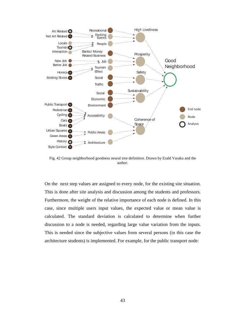
43

Fig. 42 Group neighborhood goodness neural tree definition. Drawn by Erald Varaku and the author.

On the next step values are assigned to every node, for the existing site situation.

This is done after site analysis and discussion among the students and professors.

Furthermore, the weight of the relative importance of each node is defined. In this

case, since multiple users input values, the expected value or mean value is

calculated. The standard deviation is calculated to determine when further

discussion to a node is needed, regarding large value variation from the inputs.

This is needed since the subjective values from several persons (in this case the

architecture students) is implemented. For example, for the public transport node:

GoodNeighborhood

High LivelinessRecreationalArt Related

Not Art Related

LocalsTourists

Interaction

New JobBetter Job

Horeca

Existing Stores

History

Style Context

Public Transport

PedestrianCycling

Cars

Boats

Urban Squares

Green Areas

ExcitingEvents

People

Job

TourismEffect

Social

Economic

Environment

Social

Traffic

Banks/ MoneyRelated Business Prosperity

Coherence ofSpace

Sustainability

Safety

Architecture

Accessibility

Public Areas

End node

Node

Analysis

44

Fig. 43 Value input for public transport node. Drawn by the author.

Once the values for accessibility are assigned, the process is repeated with the

weights. In previous image, the weight value of 0.26 is the result of assigning

weights to all the nodes that belong to accessibility:

Fig. 44 Accessibility node weight values. Drawn by the author.

Once the process is completed for every node, and for the three interventions

proposed (not intervene, renovate as an Art Center and demolish and build a new

Art Center) the effect on the overall neighborhood goodness is computed, as a

result of all the nodes values.

PublicTransport

0.150.850.90.80.9

2020201518

0.72

18.6 0.26

User inputs

value 0-1

weight 0-20

Mean value weight 0-1 *ex

istin

g

Mean value

Public Transport

Pedestrian

Cycling

Cars

Boats

Accessibility

0.260.230.24

0.16

0.09

45

Fig. 45 Good neighborhood value outcome. Drawn by the author.

From the benefits of the use of the neural tree, two stand out:

1- Ability to express subjective abstractions in a numeric form, which allows to be compared.

2- The user concentrates in the nodes individually, resulting in a complex network.

As a result, besides the overall value of the intervention over the end goal, a study

of the relative effect of every node is obtained. This is referred sensitivity. This

sensitivity is expressed in the value of the slope and is sometimes called the "rate

of change" because it measures the rate of change in “y” as a result of a change in

“x”. On the neural tree, the relative effect of the overall solution for each node is

revealed.

GoodNeighborhood

High LivelinessRecreationalArt Related

Not Art Related

LocalsTourists

Interaction

New JobBetter Job

Horeca

Existing Stores

History

Style Context

Public Transport

PedestrianCycling

Cars

Boats

Urban Squares

Green Areas

ExcitingEvents

People

Job

TourismEffect

Social

Economic

Environment

Social

Traffic

Banks / MoneyRelated Business Prosperity

Coherence ofSpace

Sustainability

Safety

Architecture

Accessibility

Public Areas

End node

Node

Analysis

0.830.890.95

0.740.800.91

0.590.700.84

0.860.860.86

0.700.770.85

0.780.790.81

46

Fig. 46 Sensitivity analysis. Drawn by the author.

The function of the overall performance (final node) is obtained by input of the

complete domain of values from 0 to 1.00 for every node, individually. The result

shows the influence of the node in the overall tree. In the example of the urban

analysis, the given values for the first intervention are input on the sensitivity

graphs. The nodes which present a steeper slope in the function, for the given

input, reflect the more effective fields to intervene in order to increase the end

node value (in the example, neighborhood goodness).

In figure 47, the sensitivity graphs of four of the nodes are shown. The highlighted

point in each of them is the value for the existing situation, given by the group.

The slope at that point, indicates that efforts in increasing horeca (hotel,

restaurant, café) are more beneficial for the neighborhood goodness.

sensitivityf(x)1

0 x

47

Fig. 47 Sensitivity of three nodes. Drawn by the author.

4.3 Extended decisions formulation.

Along with the criteria, the user has the means to include other architectural

decisions by the parameter definition. This is important as it does not increase the

number of goals which makes the search more expensive in computation costs.

For example, in case one of the departments is desired to be allocated in the south

façade of a building (user defined), instead of implementing it as a goal and

analyzing the distance to the south façade boundary, the parameter definition that

locates this department is fix to the value that satisfy this premise (0,00 in figure

48).

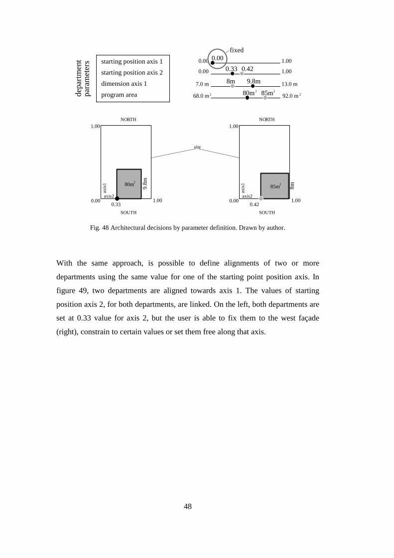
48

Fig. 48 Architectural decisions by parameter definition. Drawn by author.

With the same approach, is possible to define alignments of two or more

departments using the same value for one of the starting point position axis. In

figure 49, two departments are aligned towards axis 1. The values of starting

position axis 2, for both departments, are linked. On the left, both departments are

set at 0.33 value for axis 2, but the user is able to fix them to the west façade

(right), constrain to certain values or set them free along that axis.



dimension axis 1

program area

0.00 1.00

0.00 1.00

0.00fixed

0.00 1.00

1.00

0.33 0.42

0.33

7.0 m 13.0 m9.8m8m

9.8

m

68.0 m 92.0 m80m 85mdepa

rtm

ent

para

me

ters

NORTH

axi

s1

axis2

SOUTH

2 22 2

80m2

0.00 1.00

1.00

0.42

8m

NORTH

site

axi

s1

axis2

SOUTH

85m2

49

Fig. 49 Alignment by parameter definition. Drawn by author.

Along with these formulations, the user is able define his/her own. In this thesis,

the departments are defined by the parameter values that locate them in the site

with their sides parallel to an orthogonal coordinate system. However, custom

defined formulation is able to include irregular site orientations. For example: if

axis1 > 0.5 and axis2 < 0.6; then rotate the department.

Fig. 50 Irregular site formulation. Drawn by author.

NORTH

axis

1

axis2

SOUTH

2 22 2

80m2

0.00 1.00

1.00

0.18

8m site

85m2

0.00 1.00

1.00



dimension axis 1

program area

0.00 1.00

0.00 1.00

0.00 0.43

0.00 1.00

1.00

0.33

0.33

7.0 m 13.0 m9.8m8m

9.8

m

68.0 m 92.0 m80m 85mdepa

rtm

ent

para

me

ters

NORTH

axis

1

axis2

SOUTH

0.00

0.60

0.50

1.00

1.00

0.60

50

A specific formulation of each department helps to reduce computation costs. For

example, given a department which starting point is too close to the boundary

(close to 1), the resulted element for that solution will be out of the site boundary

limit. In order to make the algorithm more efficient, the set of values for the

starting points positions are reduced for each element regarding the minimum

dimension that they could take for axis1 and axis2. Beyond those values the

departments would always fall out of the site, so this prevents the algorithm to

compute them.

Fig. 51 Custom value range for starting position for each element. Drawn by the author.

At this point, each element is custom defined with range values that determine its

possible position in the site and its size. By customizing certain values for each of

them, the architect establishes a first order of relations, such as having some

elements in the same floor, aligned, or one on the top of other (by using the same

starting point and different height, or one in the range of the resulted element).

4.4 Other possible formulations proposed for the spatial allocation problem.

The previous formulations were intended to not limit the design freedom without

taking into account the computational cost. There are other formulations that

obtain solutions at a faster peace but with some design limitations.

0.00 0.80.

0.80

0.00 0.80.0.00 1.00

1.00 1.00

.

0.80

out ofboundary

out ofboundary

51

The first one is an attempt to reduce the number of criteria. In order to reduce the

intersections the departments are assigned step-wise. It is referred as a

constructive method, since the departments are included one by one. The first

department is assigned with the variables defined in figure 32 (starting position

axis 1 and 2, dimension axis 1 and program area). To assign the second, the

starting point is set on the contour of the first one. The next department starts on

the contour of the union of the previous. This approach is limited to departments

on the same floor.

Fig. 52 Step-wise department assignment. Drawn by the author.

To avoid overlaps, an if/else condition is implemented to locate the new

departments in places that do not intersect the previous boundary. The solutions

obtained are very dependent on the order of assignment of the departments as in

the Spiral Facility Layout Algorithm (figure 6).

To completely eliminate both, the overlaps and the intersection with the boundary

limit from the criteria, a recursive subdivision is suggested.

1 1 1

3

2

1+2 1+2 1+2+3

starting position

boundary union boundary unionboudnary point selectionand new department aggregation

boundary point selection new department aggregation

52

Fig. 53 Recursive subdivision of a rectangle in smaller rectangles. Drawn by the author.

A recurrent division of a rectangle in smaller pieces is suggested also by

Doulgerakis (2007).

Fig. 54 Polygonal subdivision. Doulgerakis 2007.

In these approaches the user interaction is reduced. There is no possibility of

locking or defining some departments locations. However, if the relations are well

defined from the beginning, the implementation of these approaches grant quick

outcomes.

12

2

3 34

53

Fig. 55 Variables and criterion summary. Drawn by the author.



dimension axis 1program area

parameters definitiondepartments

noitcesretnispalrevowith boundary

traveldistance

travelbetween

2 departments

travelbetween 3 or moredepartments

1

1-6 1-2 6-7 1-2-6-7 3-6-7union

2 3 4 5 6 7 ...

w w

w w w w w

ww

0.00 1.00

1.00

0.340.25

MULTI-OBJECTIVE OPTIMIZ ATION

54

55

CHAPTER 5

CASE STUDIES

Two cases are selected to evaluate the adequacy of the model to assist in the

creation of building layouts. The first case is used to measure the response in time

for different formulations.

5.1 Case study 1

For the first case study two sets of departments are studied. These are composed

by six and nine departments respectively. The areas are constrained to the

following domains:

Table 2 Case study 1: Departments area values.

department d1 d2 d3 d4 d5 d6 d7 d8 d9

area

80-

100

230-

260

280-

300

450-

475

350-

375

350-

375

230-

260

230-

260

250-

275

250-

275

200-

225

150-

175

150-

175

220-

250

220-

250

Fig. 56 Case study 2: Bounding box. Drawn by the author.

bounding box

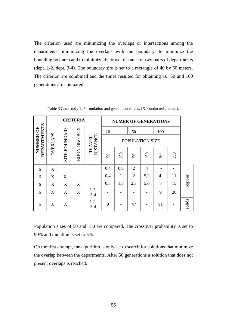
56

The criterion used are minimizing the overlaps or intersections among the

departments, minimizing the overlaps with the boundary, to minimize the

bounding box area and to minimize the travel distance of two pairs of departments

(dept. 1-2, dept. 3-4). The boundary site is set to a rectangle of 40 by 60 meters.

The criterion are combined and the times resulted for obtaining 10, 50 and 100

generations are compared.

Table 3 Case study 1: Formulation and generation values. (X: conducted attempt).

Population sizes of 50 and 150 are compared. The crossover probability is set to

90% and mutation is set to 5%.

On the first attempt, the algorithm is only set to search for solutions that minimize

the overlap between the departments. After 50 generations a solution that does not

present overlaps is reached.

NU

MB

ER

OF

D

EP

AR

TM

EN

TS

CRITERIA NUMER OF GENERATIONS

OV

ER

LAP

S

SIT

E B

OU

ND

AR

Y

BO

UN

DIN

G B

OX

TR

AV

EL

DIS

TA

NC

E

10 50 100

POPULATION SIZE

50

150

50

150

50

150

6 X 0,4 0,8 2 4 - -

regi

ons

6 X X

0,4 1 2 5,2 4 11

6 X X X 0,5 1,3 2,3 5,6 5 15

6 X X X 1-2, 3-4

- - - - 9 20

6 X X

1-2, 3-4

9 - 47 - 91 -

solid

s

57

Fig. 57 Case study 1: 6 departments; minimize overlaps. Drawn by the author.

The second criteria, intersection with boundary (figure 58) and the third, minimize

the bounding box (figure 59) are included and a sample of solutions is obtained.

Fig. 58 Case study 1: 6 departments; minimize overlaps and intersection with boundary. Drawn by the author.

Fig. 59 Case study 1: 6 departments; minimize overlaps, intersection with boundary and bounding box area. Drawn by the author.

After the first tests, the population size is set to 150, as it presented more defined

Pareto fronts. The next attempt includes the criteria referred as travel distance for

two pairs of departments (depts. 1 and 2, and depts. 3 and 4).

number of genera tions

number of populations

10 501005010 100

15050

10 5010050g10 100

150p50

10 5010050g10 100

150p50

58

Fig. 60 Case study 1: 6 departments; overlaps, boundary and travel distance after 100 generations, 150 population size. Drawn by the author.

Despite the increase in population size, the number of generations is not sufficient

to obtain clear Pareto fronts and to select a solution that satisfies all the criterion is

unachievable. Additionally, a fault in the criteria formulation is found. The

calculus of the overlaps was formulated as the difference of the summation of the

volumes of all the departments and the volume of the union.

Fig. 61 Case study 1: Minimize overlaps. Drawn by author.

On the first attempts, the use of regions was preferred due to the low computation

time required (as shown in Table 3). Therefore, the volume was substituted by the

calculus of the area.

dept 1dept 3

dept 2dept 4

Minimize overlaps

union intersection

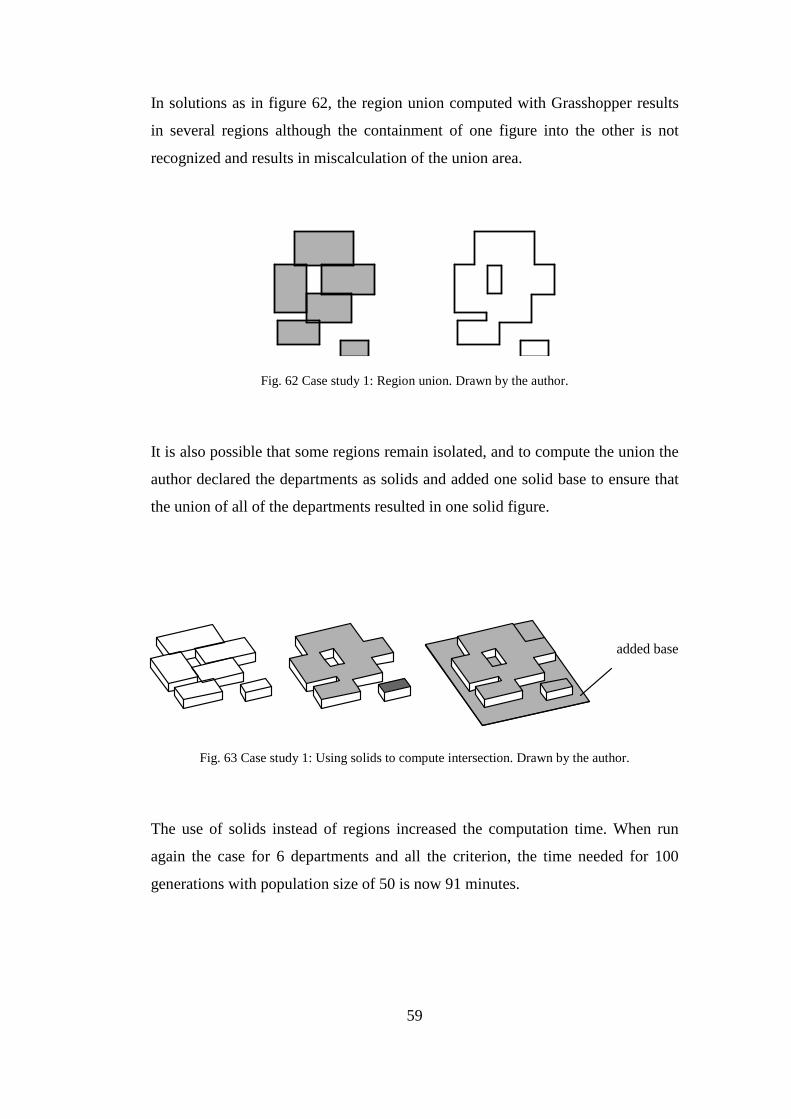
59

In solutions as in figure 62, the region union computed with Grasshopper results

in several regions although the containment of one figure into the other is not

recognized and results in miscalculation of the union area.

Fig. 62 Case study 1: Region union. Drawn by the author.

It is also possible that some regions remain isolated, and to compute the union the

author declared the departments as solids and added one solid base to ensure that

the union of all of the departments resulted in one solid figure.

Fig. 63 Case study 1: Using solids to compute intersection. Drawn by the author.

The use of solids instead of regions increased the computation time. When run

again the case for 6 departments and all the criterion, the time needed for 100

generations with population size of 50 is now 91 minutes.

added base

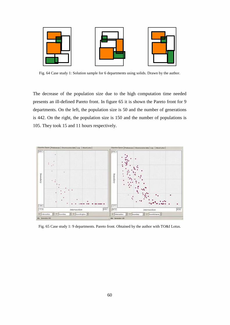
60

Fig. 64 Case study 1: Solution sample for 6 departments using solids. Drawn by the author.

The decrease of the population size due to the high computation time needed

presents an ill-defined Pareto front. In figure 65 it is shown the Pareto front for 9

departments. On the left, the population size is 50 and the number of generations

is 442. On the right, the population size is 150 and the number of populations is

105. They took 15 and 11 hours respectively.

Fig. 65 Case study 1: 9 departments. Pareto front. Obtained by the author with TO&I Lotus.

61

Fig. 66 Case study 1: Solution sample after 442 generations, 50 population size. Drawn by the author.

Fig. 67 Case study 1: Solution sample after 105 generations, 150 population size. Drawn by the author.

The increase in the population size produces higher number of solutions and a

more defined Pareto front. That is desirable to select among multiple criteria. The

sample of solutions in figure 67 show better solutions for the travel distance goal.

At last, other formulations were attempted. The first one was to use a grid for

locating the starting points of the departments. A constructive placement approach

is taken and the departments are added one by one. Once a department is added

the points of the grid contained by the department are eliminated.

Fig. 68 Constructive placement in grid network. Drawn by the author.

62

For this example a boundary site is proposed (blue shape). For 6 departments, 100

population and 30 generations some solutions are presented:

Fig. 69 Allocation of six departments in a square grid of 1m cell. Drawn by the author.

Another constructive placement approach, as explained in figure 70 is attempted.

In this case the starting point of the new department is located on the perimeter of

the previous region. The results are notably dependent on the incorporation order.

Recursive subdivision test (figure 71) presents an improvement in the algorithm

performance, but design limitations arise, as it is difficult to control the exact

number of rectangles obtained and their proportions.

Fig. 70 Constructive placement. 8 departments of 60 m2. Drawn by the author.

Fig. 71 Recursive divisions of a rectangle with three points resulting in 10 subdivisions. Drawn by the author.

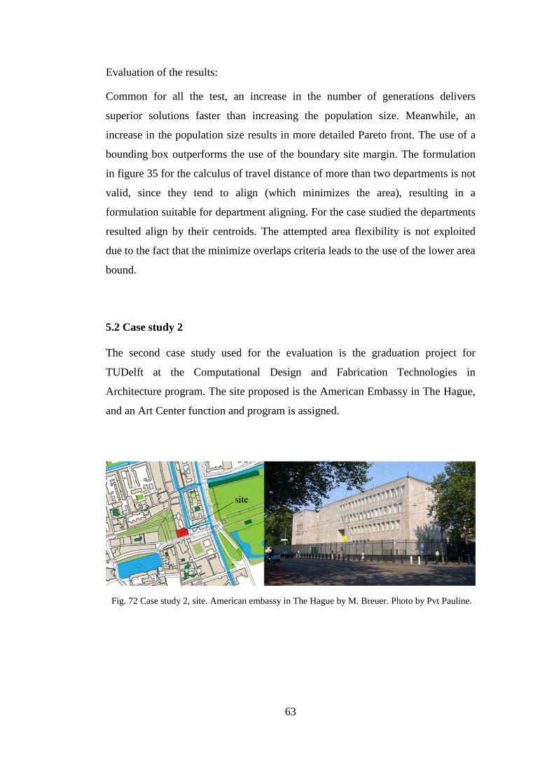
63

Evaluation of the results:

Common for all the test, an increase in the number of generations delivers

superior solutions faster than increasing the population size. Meanwhile, an

increase in the population size results in more detailed Pareto front. The use of a

bounding box outperforms the use of the boundary site margin. The formulation

in figure 35 for the calculus of travel distance of more than two departments is not

valid, since they tend to align (which minimizes the area), resulting in a

formulation suitable for department aligning. For the case studied the departments

resulted align by their centroids. The attempted area flexibility is not exploited

due to the fact that the minimize overlaps criteria leads to the use of the lower area

bound.

5.2 Case study 2

The second case study used for the evaluation is the graduation project for

TUDelft at the Computational Design and Fabrication Technologies in

Architecture program. The site proposed is the American Embassy in The Hague,

and an Art Center function and program is assigned.

Fig. 72 Case study 2, site. American embassy in The Hague by M. Breuer. Photo by Pvt Pauline.

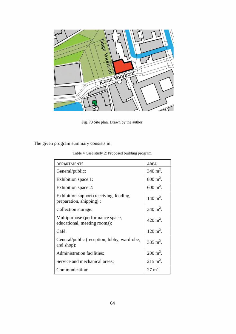
64

Fig. 73 Site plan. Drawn by the author.

The given program summary consists in:

Table 4 Case study 2: Proposed building program.

DEPARTMENTS AREA

General/public: 340 m2.

Exhibition space 1: 800 m2.

Exhibition space 2: 600 m2.

Exhibition support (receiving, loading, preparation, shipping) :

140 m2.

Collection storage: 340 m2.

Multipurpose (performance space, educational, meeting rooms):

420 m2.

Café: 120 m2.

General/public (reception, lobby, wardrobe, and shop):

335 m2.

Administration facilities: 200 m2.

Service and mechanical areas: 215 m2.

Communication: 27 m2.

65

The site is formulated as a two dimension domain.

Fig. 74 Case study 2: Site definition as a two dimension domain. Drawn by the author.

As the case explores the solutions in three dimensions, the variables definition

includes the assignment of the departments to different floors and the possibility

to cover one or two storeys (in figure 75, starting floor and number of floors). The

ceiling height is set to 5 meters for all of the departments.

Fig. 75 Case study 2: variables definition. Drawn by the author.

Some of the departments are (user) constrained to certain floors. For example, the

entrance and the shop are locked to the ground floor. Some are constrained to a

starting position axis 1starting position axis 2dimension axis 1program areastarting floornumber of floorsceiling height

0 1

0

0 (0 to 2)1 (1,2)

5 m

0 1

0.54

10 2020

170 230200mm2

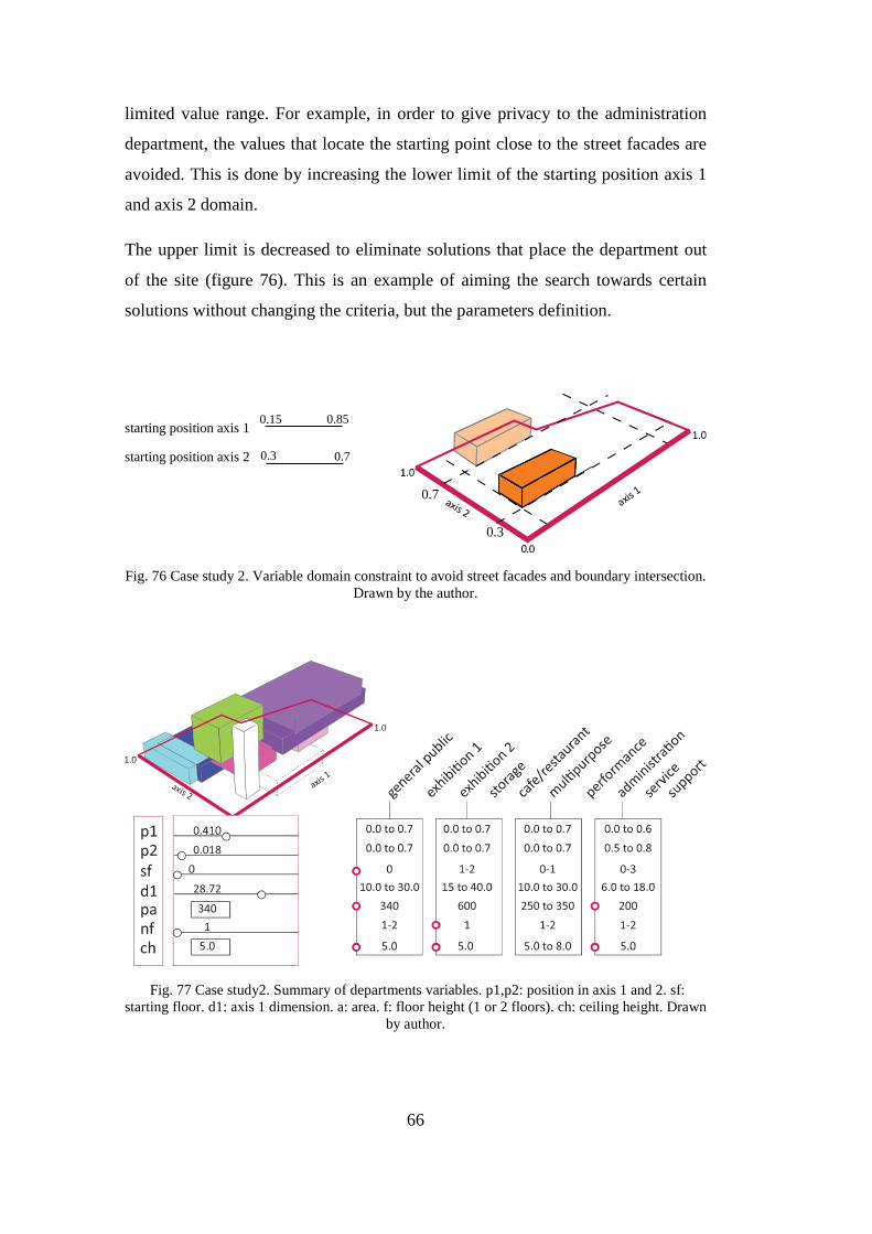
66

limited value range. For example, in order to give privacy to the administration

department, the values that locate the starting point close to the street facades are

avoided. This is done by increasing the lower limit of the starting position axis 1

and axis 2 domain.

The upper limit is decreased to eliminate solutions that place the department out

of the site (figure 76). This is an example of aiming the search towards certain

solutions without changing the criteria, but the parameters definition.

Fig. 76 Case study 2. Variable domain constraint to avoid street facades and boundary intersection. Drawn by the author.

Fig. 77 Case study2. Summary of departments variables. p1,p2: position in axis 1 and 2. sf: starting floor. d1: axis 1 dimension. a: area. f: floor height (1 or 2 floors). ch: ceiling height. Drawn

by author.

axis1

0.3

0.7


starting position axis 20.3 0.7

0.15 0.85

67

With the defined variable for the set of departments, the algorithm is run for the

two first criteria: avoid overlaps and do not exceed the boundary site. On figure 78

a sample of solutions is presented, for which the criterion are to be minimized.

Fig. 78 Case study 2.Two goals. 150 population, 200 generations. Drawn by the author.

The travel distance is included as a new criteria for the following departments:

Exhibition Gallery 1 and 2; Multipurpose and Performance 1; Administration and

Service. The same weight is given to all of them.

A rotation degree is assigned if the department starting point is close to

Smidswater street (figure 74) as an attempt to align them to the site´s shape in that

corner. If the starting position in axis 1(p1) is larger than 0.6 and the starting

position in axis 2 (p2) is larger than 0,5, then the department rotates 0.25 radians

counterclockwise. A solution sample is shown in the next figure.

68

Fig. 79 Case study2. Three goals. 200 population, 20 generations. Drawn by the author.

A new set of elements, in this case voids, is included as part of the architectonic

idea for the project. These are fixed elements and the new criteria is not to

intersect them.

Fig. 80 Case study 2. Incorporation of voids to the design. Drawn by the author.

The resulting Pareto front for these four goals results unclearly defined and with

an average of 2,3 seconds per solution, the analysis of 400 generations of 200

solutions per population, resulted in more than two days.

69

Fig. 81 Case Study 2. Four goals Pareto front after 400 generations. Drawn by the author.

In order to increase the performance, an evaluation of the algorithm´s parts was

performed to evaluate their response time. The calculation of the intersections of

the departments took the highest computation power. Several attempts were

evaluated using regions, meshes and solids. The regions resulted in inconclusive

due to the errors in calculations if one appeared completely inside other.

Fig. 82 Region included in region is not computed as intersection in Grasshopper. Drawn by the author.

The meshes intersection in Grasshopper presented a flaw in its calculations. In

figure 83 an overview of the outcome of the union using mesh, simple mesh and

solid objects is shown. Due to this problem, the use of meshes was dismissed.

Pareto front

travel voidsintersections boundary

70

Fig. 83 Case study 2. Mesh calculation flaw in Grasshopper. Drawn by the author.

Despite these difficulties, the use of the tool was helpful for the formulation of the

relations and a set of solutions was obtained. From these solutions the following

layout was selected.

Fig. 84 Solution outcome example. Drawn by the author.

71

The solution obtained satisfied the previously formulated criteria:

1- It presented a small overlap amount.

2- All of the departments were contained within the site boundary.

3- -The solution granted the required departments horizontally adjacent

(multipurpose and performance), or vertically (exhibition one and two, and

administration and service), according the travel distance formulation.

The study of each department individually, and the reflection on each relation to

define the problem formulation together with the criteria definition provides deep

knowledge of the project essence, which is not achieved with other methods.

Besides, clear criteria definition and grading the solutions facilitates the

understanding to other people, like the client, who can include his/her criteria and

weights in an explicit manner.

72

73

CHAPTER 6

CONCLUSIONS

This study addresses the limited design freedom of previous spatial allocation

studies, and proposes new formulations and the use of Intelligent Design Objects

as a model to overcome these limitations.

Previous studies approach the problem locating modules in a grid, computing the

distances between departments and improving the obtained solutions. It is useful

for certain scenarios, but results are too rigid or not flexible for architecture

design. In this thesis, the author proposes a model that takes into account

variances in the program areas, and establishes relative importance among the

departments to overcome that rigidity of previous studies. Special attention is put

to the problem formulation, in order to make it suitable for different design

problems and building types.

The proposed variable formulations make the computation expensive. Increases in

the number of criteria result in much longer computational time and undefined

Pareto fronts. The simplification of the parameters brings faster results, but limits

the design freedom. It is the user´s duty to prepare the proper formulation for the

task.

From the selected optimization plugins in Grasshopper (Octopus, Goat, Galapagos

and TO&I Lotus), the first two could not stand the high computation and failed to

obtain results. Galapagos, on the other hand, coped with the high number of

parameters, but the criteria had to be combined into a single cost function making

the result highly dependent on the weights and unreliable. The only tool that

74

managed the high number of parameters and the multiple criteria was TO&I

Lotus.

The method proposed helps to visualize and evaluate different solutions and to

conceive the different department relations at an early stage of building layout.

Besides, at all times the solutions are numerically graded and provide, also to the

client, an understanding of their “goodness”. Once a solution is selected, is

possible to designate new criteria, such as yearly sun radiation, and define a set of

transformations, such as scaling or movement of the departments to adapt the

solution towards this new goal.

The graphic interface facilitates interaction with the user, and makes possible to

move and lock departments and explore different relations. For further

researchers, the use of a programing language is advised to overcome the

computing limitations of the tool.

Fifty years from Armor and Bufa research in 1964, and still the spatial allocation

problem remains more interesting to researches than to practitioners. This is in

part due to the difficulty of the problem formulation and also to the architectural

practice itself. The first one, in the literature, is approached by a simplification of

the problem. The formulation of a grid to locate the elements and to assign them

to modules has been part of the formulation of most of the studies. Making the

architectural spatial relations look alike distance cost functions drives designers

away from these methods.

In this study, the model is not intended to serve as an automatization of the task.

Instead, an iterative improvement process is proposed. This is achieved by two

means: the first is user interaction. The method proposes a user defined

formulation of the departments’ areas, proportions and (as in the second case

study) their floor position. This step is aimed to provide a reflection on the

architectural program and, at the same time, constrain the search. The second, is a

constant numeric and visual feedback of the results.

75

The process is refined after some solutions are obtained. Besides, at any moment,

the user is able to incorporate new architectural decisions (as the inclusion of

voids in the last example).

The Intelligent Design Objects method contemplates the possibility of further

assistance for the designer. Once the layout configuration is decided, a new set of

transformations (alignment, scaling…) is to be paired to new defined criteria

(solar analysis, structure…).

Further studies should be carried to reduce limitations related with computational

time. The first guideline is to adopt a programing language to cope with the

mentioned computation. To correct the meshes intersections and use them should

cut down the needed time by three or four times, according the tests run. A higher

number of departments considered should be studied to determine the validity

limit of the method. At last, an elaboration to combine several of the approaches

shown into the same project should be considered. For larger set of departments,

the suggested workflow is to set them into larger groups, for example, regarding

their function, and proceed to arrange them within the group. The possibilities of

neural tree are also presented in this thesis. However, the focus was put on multi-

objective optimization, rather than combining the criteria into one single

objective. An example is included to show the potential of this method. Further

studies should overcome the computational cost limitations and compare the

results of both approaches.

To sum up, the use of Intelligent Design Objects method for the spatial allocation

problem proposed in this thesis has proved its validity, and some limitations. It

has also shown the potential for further criteria elaborations.

76

77

LIST OF REFERENCES

Akin, O., Dave, B. and Pithavadian, S., 1992. Heuristic generation of layouts

(HeGel): based on a paradigm for problem structuring, Environment and Planning

B 19: 33-59.

Arabacioglu, B.C., 2009. Using fuzzy inference system for architectural space

analysis.

Baykan, C.A. and Fox, M.S., 1997. Spatial synthesis by disjunctive constraint

satisfaction. AI EDAM 11(4):245-262.

Bittermann, M.S., 2009. "Intelligent Design Objects (IDO) A cognitive approach

for performance based design," PhD Thesis, Dept. of Building Technology, Delft

University of Technology, Delft, The Netherlands.

Buffa, E.S., Armor, G.S. and Vollman, T.E., 1964. Allocating facilities with

CRAFT, Harvard Business Review 42(2): 136-140.

Caldas, L., 2008. Generation of energy-efficient architecture solutions applying

GENE_ARCH: An evolution-based generative design system

Ciftcioglu, O., Bittermann, M.S., 2009. Adaptive formation of Pareto front in

evolutionary multi-objective optimization. In: Santos, W.P.d. (ed.): Evolutionary

Computation. In-Tech, Vienna 417-444.

Deb, K., Pratap, A., Agarwal, S., Meyarivan, T., 2000. A fast and elitist multi-

objective genetic algorithm: NSGA-II. IEEE Transactions on Evolutionary

Computation 6, 182-197.

Deb, K., 2001. Multi-objective Optimization using Evolutionary Algorithms, John

Wiley & Sons.

78

Doran, J., Parberry, I., 2010. Controlled Procedural Terrain Generation Using

Software Agents.

Doulgerakis, A., 2007. Genetic Programming + Unfolding Embryology in

Automated Layout Planning.

Eastman, C.M., 1973. Automated space planning. Artificial Intelligence 4:41- 64.

Ellen Yi-Luen Do and M.D. Gross.,1997. Tools for Visual and Spatial Analysis of

CAD Models. Computer Assisted Architectural Design Futures '97, Kluwer

Academic Publisher, pp.189-202.

Galle, P. 1981. An algorithm for exhaustive generation of building floor plans.

Communications of the ACM 24, 12, 813–825.

Gero, J.S., 1977. Note on "Synthesis and optimization of small rectangular floor

plans" of Mitchell, Steadman, and Liggett, Environment and Planning B 4:81-88.

Grason, J., 1971. An approach to computerized space planning using graph

theory, Proceedings of the Design Automation Workshop, Association for

Computing Machinary, New York.

Graves, G.W. and Whinston, A., 1970. An algorithm for the quadratic assignment

problem, Management Science, 17(3): 453-471.

Hatice, E., Eldemir, S.F., 2010. Spiral Facility Layout Generation And

Improvement Algorithm.

Hillier, B. & Hanson, J., 1984. The Social Logic of Space, Cambridge: Cambridge

University Press.

Hokoda, W., 1982. RENDER-3: Graphics Digitizing and Rendering System,

Master's Thesis, School of Architecture and Urban Planning, University of

California

Indraprastha, A. and Shinozakim M., 2008. Elaboration Model for Mapping

Architectural Space.

79

Jensen, P. A., 2004. Facility Layout Add-in [Online], Available:

https://www.me.utexas.edu/~jensen/ORMM/omie/computation/unit/lay_add/lay_a

dd.html [03 Feb 2014].

Jo, J.H. and Gero, J.S., 1998. Space Layout Planning using an Evolutionary

Approach

Khokhani, K.H., Patel, A.M., 1977. The chip layout problem: A placement

procedure for lsi. Proceeding DAC’77 Proceedings of the 14th Design

Automation Conference, pp. 291-297.

Kim, H., Jun, C., Cho, Y. and Kim, G., 2008. Indoor spatial analysis using space

syntax, Department of Geoinformatics, University of Seoul.

Koller, D., Friedman, N., 2009. Probabilistic Graphical Models: Principles and

Techniques, edited by MIT Press.

Lee, R. B. and Moore, J. M. , 1967. CORELAP - Computerized Relationship

Layout Planning. Journal of Industrialized Engineering 18, No. 3, March.

Liggett, R.S., 1980. The quadratic assignment problem: an analysis of

applications and solution strategies, Environment and Planning B 7: 141-162.

Liggett, R.S., 1985. Optimal spatial arrangement as a quadratic assignment

problem, in J.S. Gero, (ed.), Design Optimization, Academic Press, New York,

pp. 1-40.

March, L., and Steadman, P., 1971. Spatial allocation procedures. In The

Geometry of Environment. MIT Press, ch. 13,303–317.

Merrell, P., Schkufza, E., Koltun, V., 2010. Computer-Generated Residential

Building Layouts.

Michalek, J.J., Choudhary, R., and Papalambros, P.Y., 2002, Architectural layout

design optimization.

80

Mitchell, W.J. et al., 1976. Synthesis and optimization of small rectangular floor

plans, Environment and Planning B 3, pp. 37-70.

Morabito, R., Morales, S., 1998. “A simple and effective recursive procedure for

manufacturer´s pallet loading problem.” Journal of the Operational Research

Society 19, 819-828.

Nourian, P, Rezvani, S., and Sariyildiz, S., 2013."Designing with Space Syntax."

In Computation and Performance - Proceedings of the 31st eCAADe Conference,

357-365. Vol. 1.

Scheithauer, G., Sommerweiß, U., 1996. Heuristics for the Rectangle Packing

Problem.

Seehof, J.M and W. O. Evans, 1972. “Automated Layout Design Program”,

Journal of Industrial Engineering, 18, 240-248.

Shaviv, E., 1986. Layout design problems: systematic approaches. CAAD Futures

Digital Proceedings, ch 3.

Sullivan F., Beichl, I., 2000. The Metropolis Algorithm. IDA/Center for

Computing Science.

Togelius, J., Yannakakis, G.N., Stanle K.O., 2010. Cellular automata for real-time

generation of infinite cave levels.

Weinzapfel, G. and S. Handel, 1975. "IMAGE: Computer Assistant for

Architectural Design" in Spatial Synthesis in Computer-Aided Building Design

ed. C. Eastman. pp 61-68 New York: Wiley.

Yoon, K.B. and Coyne, R.D., 1992. Reasoning about spatial constraints,

Environment and Planning B 19:243-266.

Documents

intelligent design objects applied to the spatial ...etd.lib.metu.edu.tr/upload/12617003/index.pdf · INTELLIGENT DESIGN OBJECTS APPLIED TO THE SPATIAL ALLOCATION ... layout organization