1

Spatial-temporal Database and moving objects management

2

Outlines

Introduction Background knowledge Spatial database Spatial-temporal database Moving objects management Conclusions

3

Introduction

4

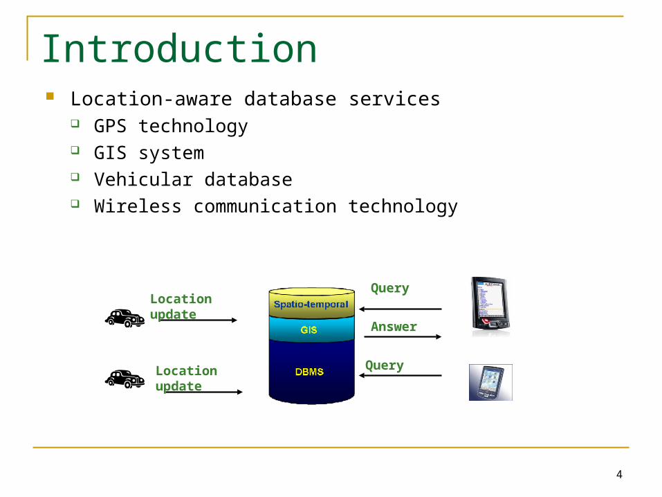
Introduction Location-aware database services

GPS technology GIS system Vehicular database Wireless communication technology

Location update

Location update

Query

Query

Answer

5

Introduction

Location-based applications Traffic monitoring and management Location-based store (services) find and advertisement People cooperation and communication

6

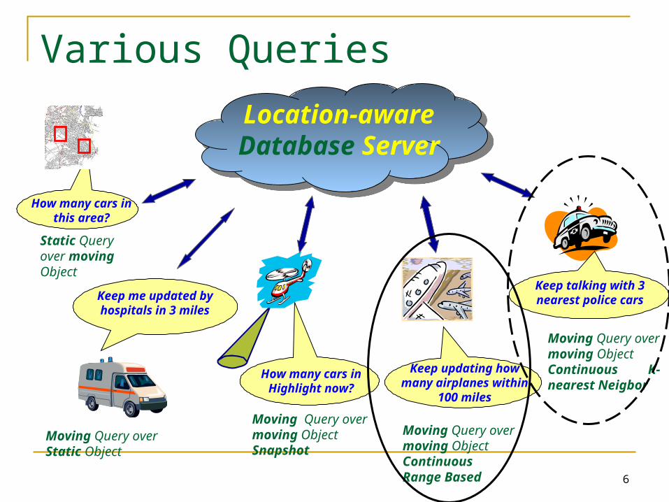
Various Queries

How many cars in this area?

Static Query over moving Object

Location-aware Database Server

Keep talking with 3 nearest police cars

Moving Query over moving Object Continuous K-nearest Neigbor

How many cars in Highlight now?

Moving Query over moving Object Snapshot

Moving Query over Static Object

Keep me updated by hospitals in 3 miles

Keep updating how many airplanes within

100 miles

Moving Query over moving Object Continuous Range Based

7

Target Query Moving Continual Queries over moving object

(MCQ)

Generalization of Moving and Static Queries

Continuous nature1 continuous query = a sequence of snapshot queries with some frequency

Range-based or kNN

8

Background knowledge

9

History of Database Technology

1960s: Data collection, database creation, IMS and network DBMS

1970s: Relational data model, relational DBMS implementation

1980s: RDBMS, advanced data models (extended-relational, OO, deductive, etc.) and application-oriented DBMS (spatial, scientific, engineering, etc.)

1990s—2000s: Data mining and data warehousing, multimedia databases, and Web databases

10

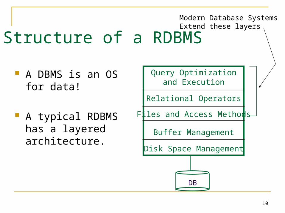
Structure of a RDBMS

A DBMS is an OS for data!

A typical RDBMS has a layered architecture.

Query Optimizationand Execution

Relational Operators

Files and Access Methods

Buffer Management

Disk Space Management

DB

Modern Database SystemsExtend these layers

11

Index Methods for RDBMS

Hashing Methods

B-tree family

Both of them are one-dimensional

12

B+-tree

Records must be ordered over an attribute

Queries exact match or range queries over the indexed

attribute find the name of the student with SID=dr868301 find all students with gpa between 3.00 and 3.5

13

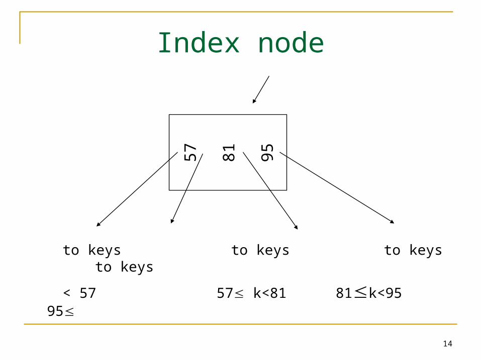
B+-tree:properties

“B” for balance! Each node contains up to n-1 search key

values and n pointers A nonleaf node may hold up to n pointers

and must hold at least Two types of nodes: index nodes and data

nodes; each node is 1 page (disk based method)

2/n

14

57

81

95

to keys to keys to keys to keys

< 57 57 k<81 81k<95 95

Index node

15

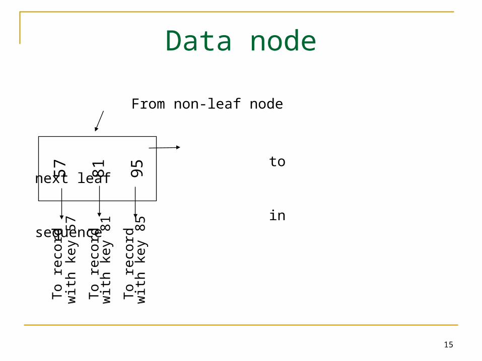
Data node5

7

81

95

To r

eco

rd

wit

h k

ey 5

7

To r

eco

rd

wit

h k

ey 8

1

To r

eco

rd

wit

h k

ey 8

5

From non-leaf node

to next leaf

in sequence

16

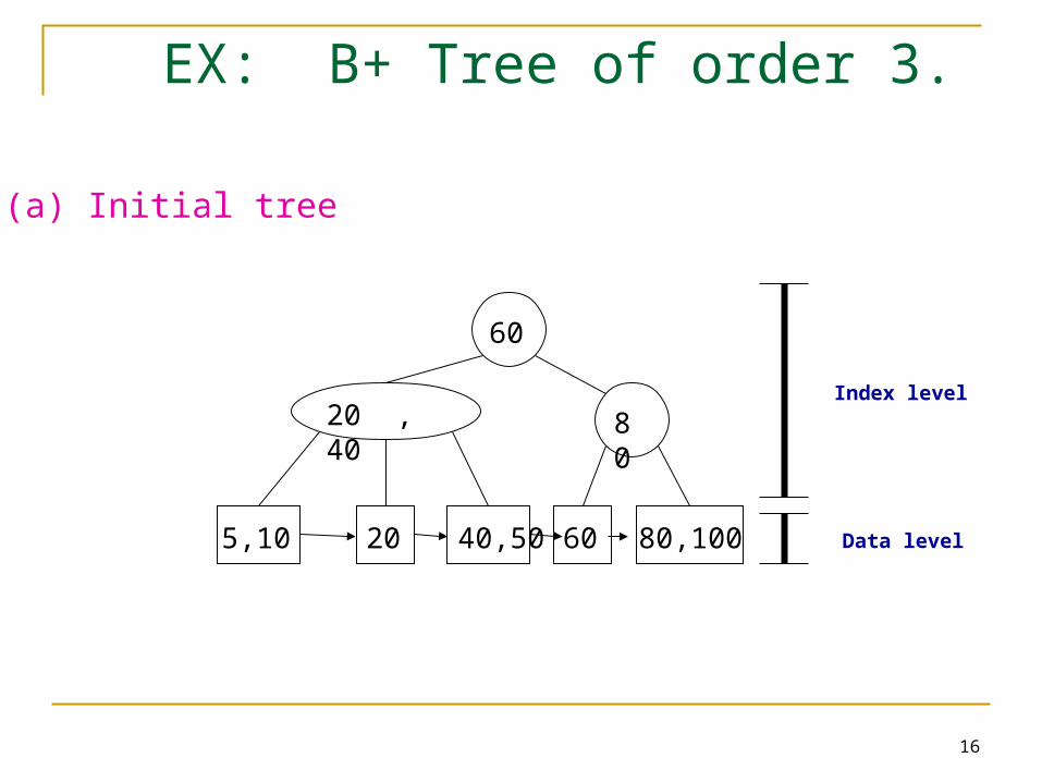
EX: B+ Tree of order 3.

(a) Initial tree

60

80

20 , 40

205,10 6040,50 80,100

Index level

Data level

17

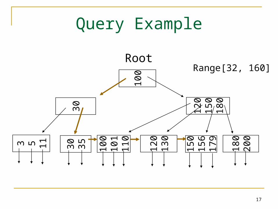
Query Example

Root

100

120

150

180

30

3 5 11

30

35

100

101

110

120

130

150

156

179

180

200

Range[32, 160]

18

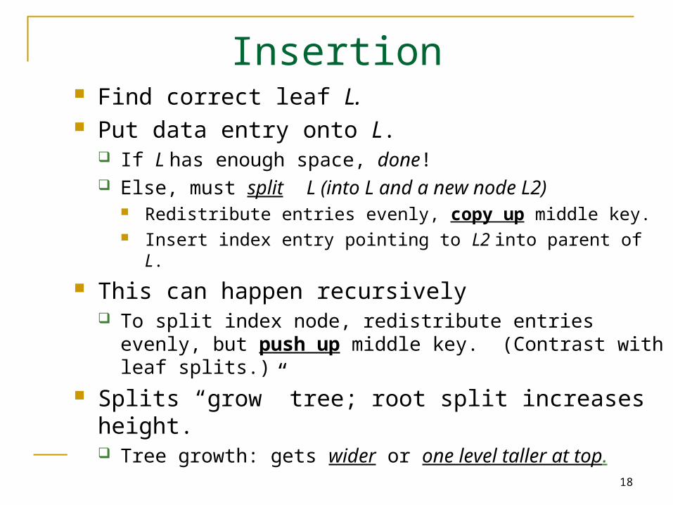
Insertion Find correct leaf L. Put data entry onto L.

If L has enough space, done! Else, must split L (into L and a new node L2)

Redistribute entries evenly, copy up middle key. Insert index entry pointing to L2 into parent of L.

This can happen recursively To split index node, redistribute entries evenly, but push

up middle key. (Contrast with leaf splits.) Splits “grow” tree; root split increases height.

Tree growth: gets wider or one level taller at top.

19

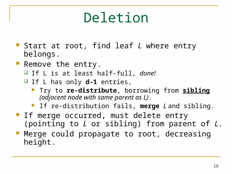
Deletion

Start at root, find leaf L where entry belongs. Remove the entry.

If L is at least half-full, done! If L has only d-1 entries,

Try to re-distribute, borrowing from sibling (adjacent node with same parent as L).

If re-distribution fails, merge L and sibling. If merge occurred, must delete entry (pointing to L or

sibling) from parent of L. Merge could propagate to root, decreasing height.

20

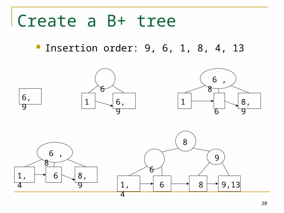
Create a B+ tree Insertion order: 9, 6, 1, 8, 4, 13

6, 9

1

6

6, 9

1

6 , 8

6 8, 9

1, 4

6 , 8

6 8, 9

8

61, 4

9,138

6 9

21

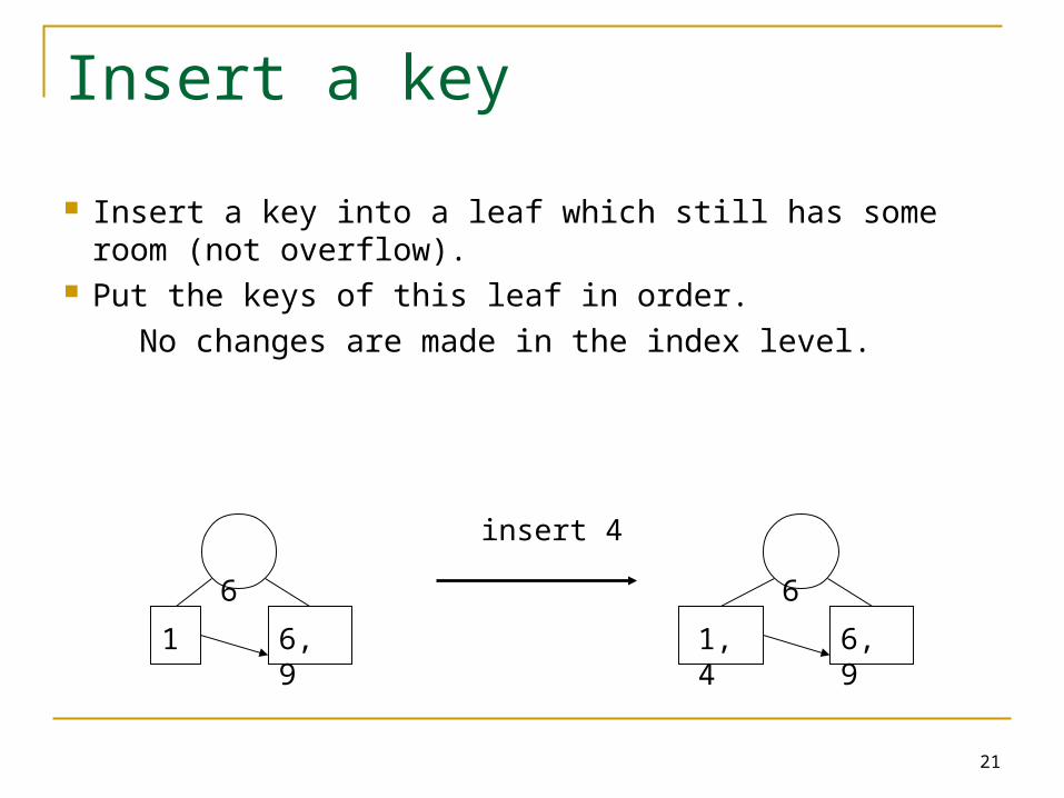
Insert a key

Insert a key into a leaf which still has some room (not overflow).

Put the keys of this leaf in order.

No changes are made in the index level.

1

6

6, 9

1, 4

6

6, 9

insert 4

22

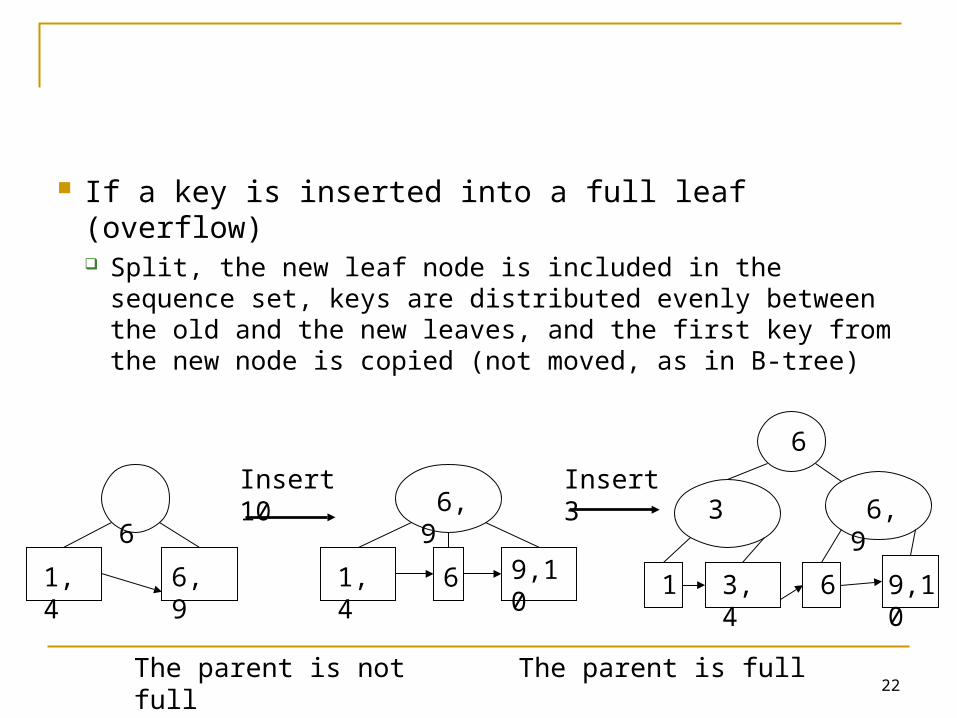
If a key is inserted into a full leaf (overflow) Split, the new leaf node is included in the sequence

set, keys are distributed evenly between the old and the new leaves, and the first key from the new node is copied (not moved, as in B-tree)

1, 4

6

6, 9

1, 4

6, 9

6

The parent is not full The parent is full

Insert 10

9,10

Insert 3

1

3

6 9,103, 4

6

6, 9

23

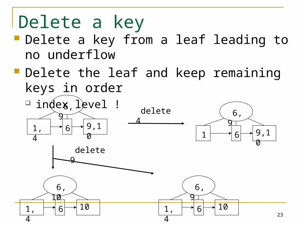
Delete a key Delete a key from a leaf leading to no underflow Delete the leaf and keep remaining keys in

order index level !

delete 4

1, 4

6, 9

6 9,10 1

6, 9

6 9,10

delete 9

1, 4

6, 10

6 10 1, 4

6, 9

6 10

24

Spatial database

25

Introduction

A common technology for some Applications: GIS (geographic/geo-referenced data) VLSI design (geometric data) modeling complex phenomena (spatial data)

All need to manage large collections of relatively simple spatial objects

26

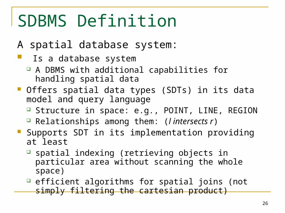
SDBMS DefinitionA spatial database system: Is a database system

A DBMS with additional capabilities for handling spatial data

Offers spatial data types (SDTs) in its data model and query language Structure in space: e.g., POINT, LINE, REGION Relationships among them: (l intersects r)

Supports SDT in its implementation providing at least spatial indexing (retrieving objects in particular area

without scanning the whole space) efficient algorithms for spatial joins (not simply filtering

the cartesian product)

27

Modeling

Assume 2-D and GIS application, two basic things need to be represented:

Objects in space: cities, forests, or rivers single objects

Coverage/Field: say something about every point in space (e.g., partitions, thematic maps)

spatially related collections of objects

28

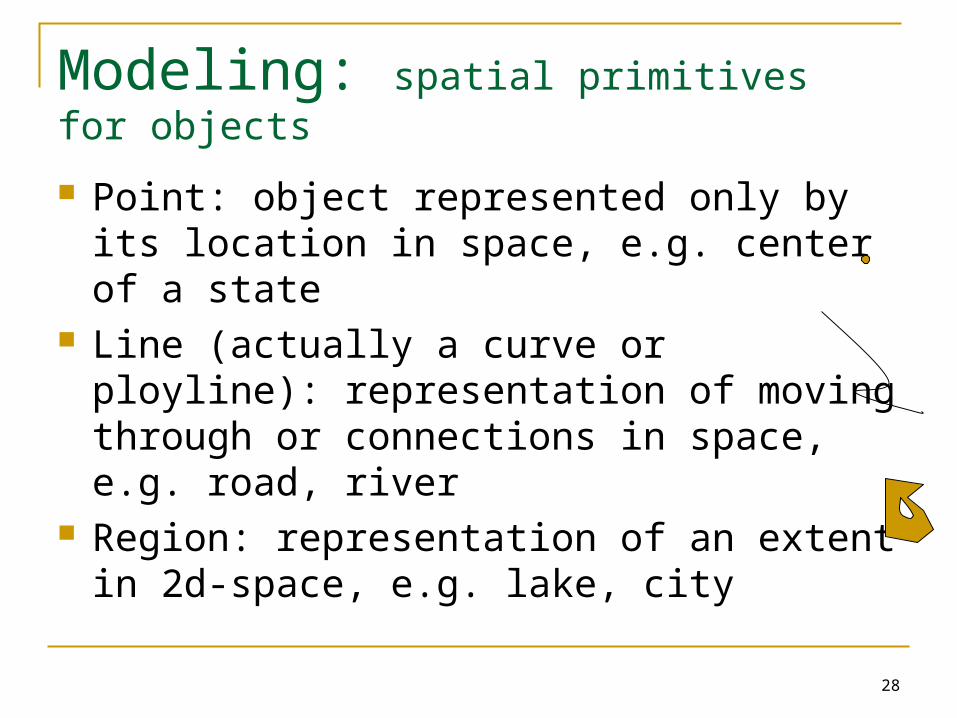
Modeling: spatial primitives for objects

Point: object represented only by its location in space, e.g. center of a state

Line (actually a curve or ployline): representation of moving through or connections in space, e.g. road, river

Region: representation of an extent in 2d-space, e.g. lake, city

29

Modeling: spatial relationships

Topological relationships: e.g. adjacent, inside, disjoint. Are invariant under topological transformations

like translation, scaling, rotation

Direction relationships: e.g. above, below, or north_of, sothwest_of, …

Metric relationships: e.g. distance

30

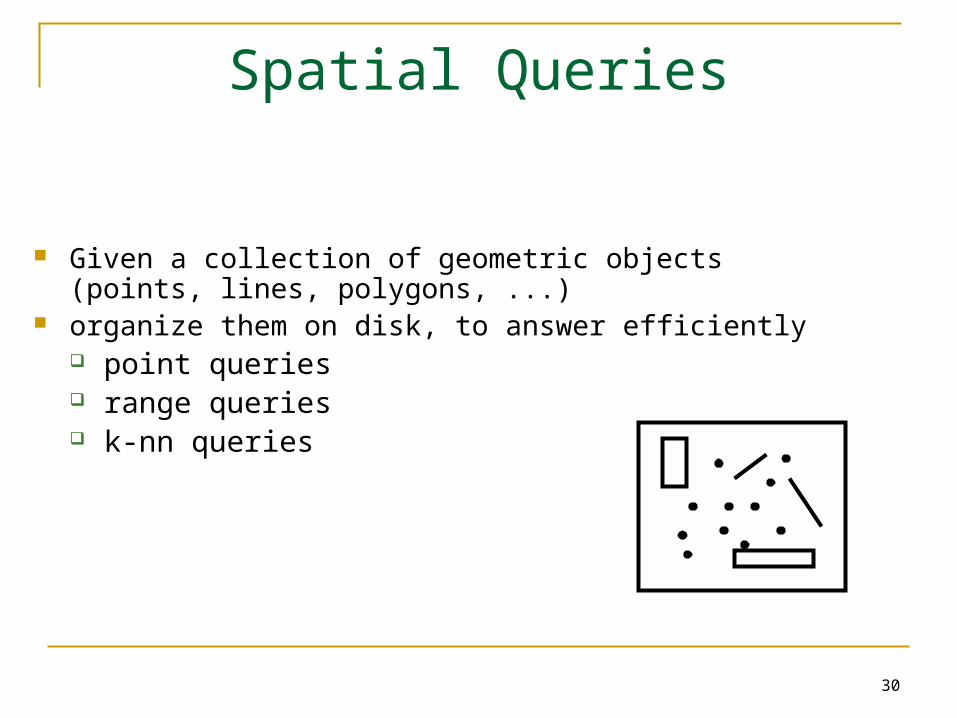
Spatial Queries

Given a collection of geometric objects (points, lines, polygons, ...)

organize them on disk, to answer efficiently point queries range queries k-nn queries

31

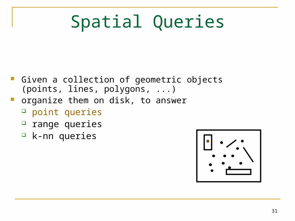
Spatial Queries

Given a collection of geometric objects (points, lines, polygons, ...)

organize them on disk, to answer point queries range queries k-nn queries

32

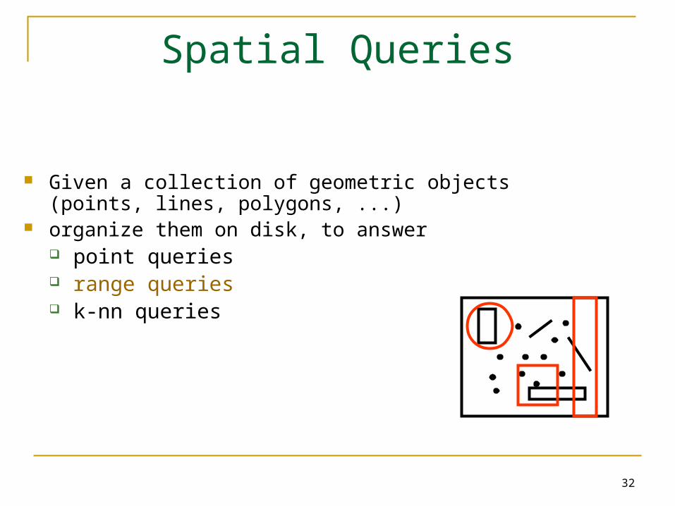
Spatial Queries

Given a collection of geometric objects (points, lines, polygons, ...)

organize them on disk, to answer point queries range queries k-nn queries

33

Spatial Queries

Given a collection of geometric objects (points, lines, polygons, ...)

organize them on disk, to answer point queries range queries k-nn queries

34

Access Methods

Discussed in the course Grid file K-d tree Z curve R-tree

35

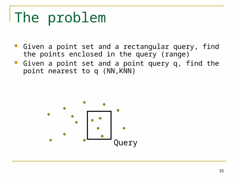
The problem

Given a point set and a rectangular query, find the points enclosed in the query (range)

Given a point set and a point query q, find the point nearest to q (NN,KNN)

Query

36

Grid File

Idea: Use a grid to partition the space each cell is associated with one page

Two disk access principle

37

Grid File

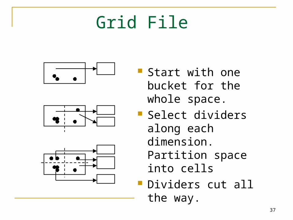
Start with one bucket for the whole space.

Select dividers along each dimension. Partition space into cells

Dividers cut all the way.

38

Grid File

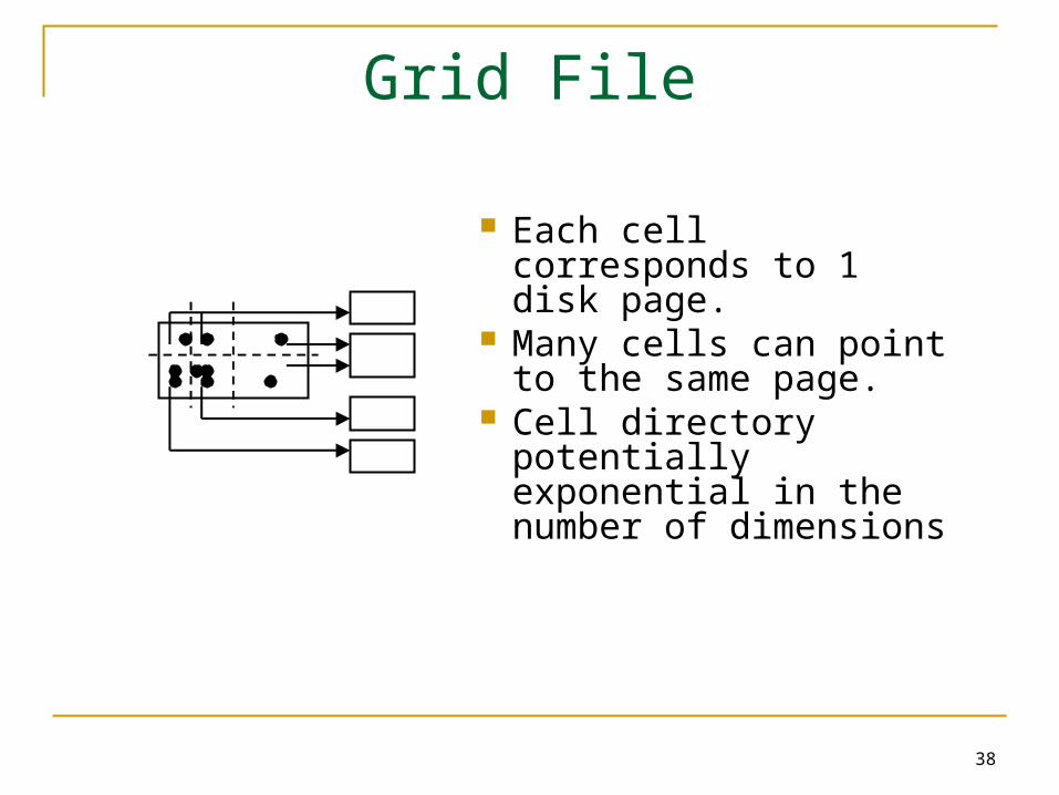
Each cell corresponds to 1 disk page.

Many cells can point to the same page.

Cell directory potentially exponential in the number of dimensions

39

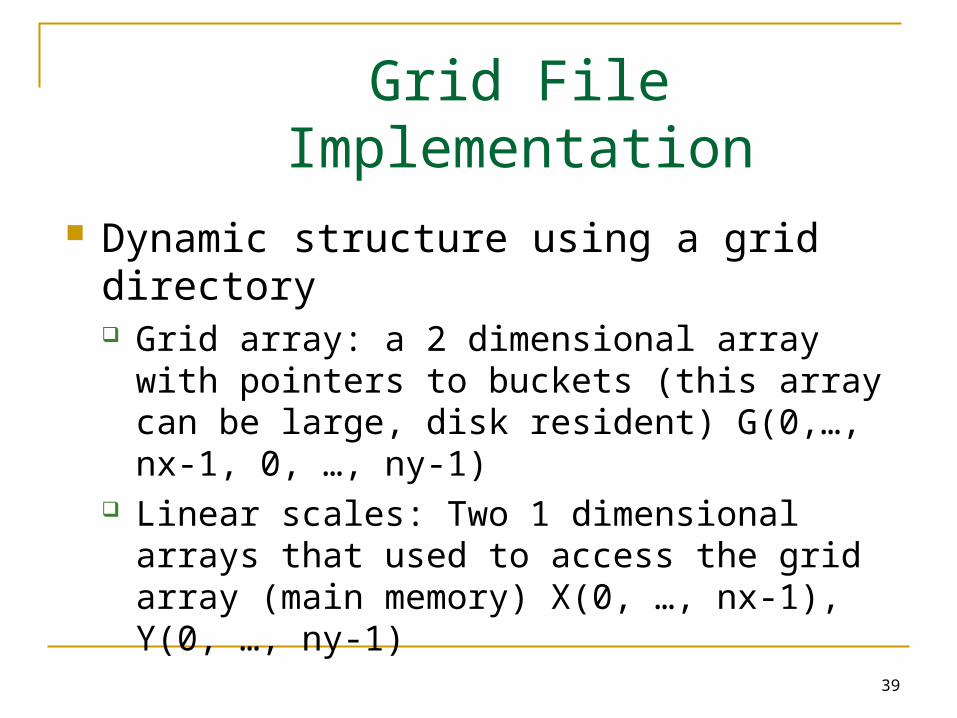
Grid File Implementation

Dynamic structure using a grid directory Grid array: a 2 dimensional array with pointers to

buckets (this array can be large, disk resident) G(0,…, nx-1, 0, …, ny-1)

Linear scales: Two 1 dimensional arrays that used to access the grid array (main memory) X(0, …, nx-1), Y(0, …, ny-1)

40

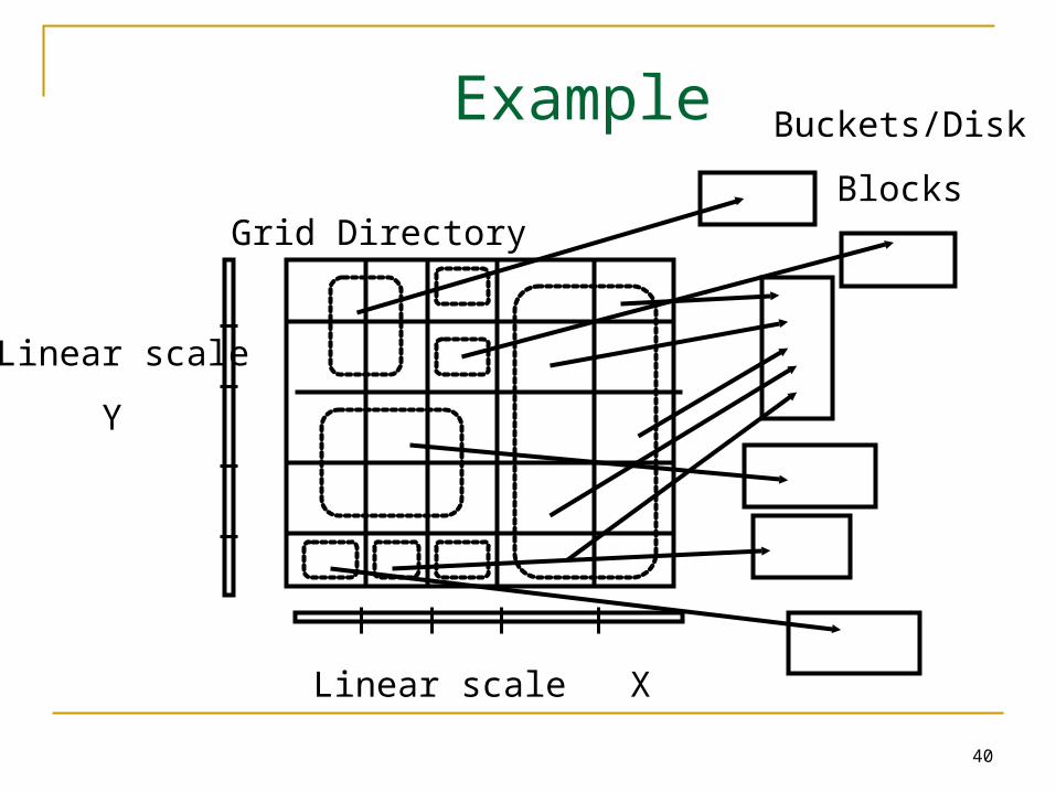
Example

Linear scale X

Linear scale

Y

Grid Directory

Buckets/Disk

Blocks

41

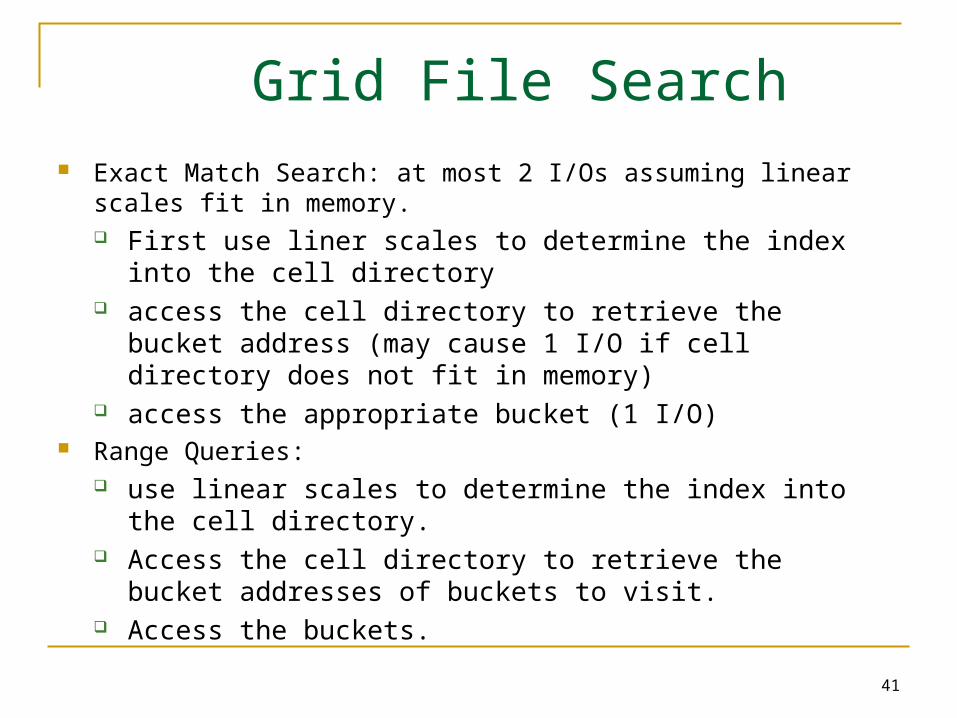
Grid File Search Exact Match Search: at most 2 I/Os assuming linear scales fit in

memory. First use liner scales to determine the index into the cell

directory access the cell directory to retrieve the bucket address (may

cause 1 I/O if cell directory does not fit in memory) access the appropriate bucket (1 I/O)

Range Queries: use linear scales to determine the index into the cell directory. Access the cell directory to retrieve the bucket addresses of

buckets to visit. Access the buckets.

42

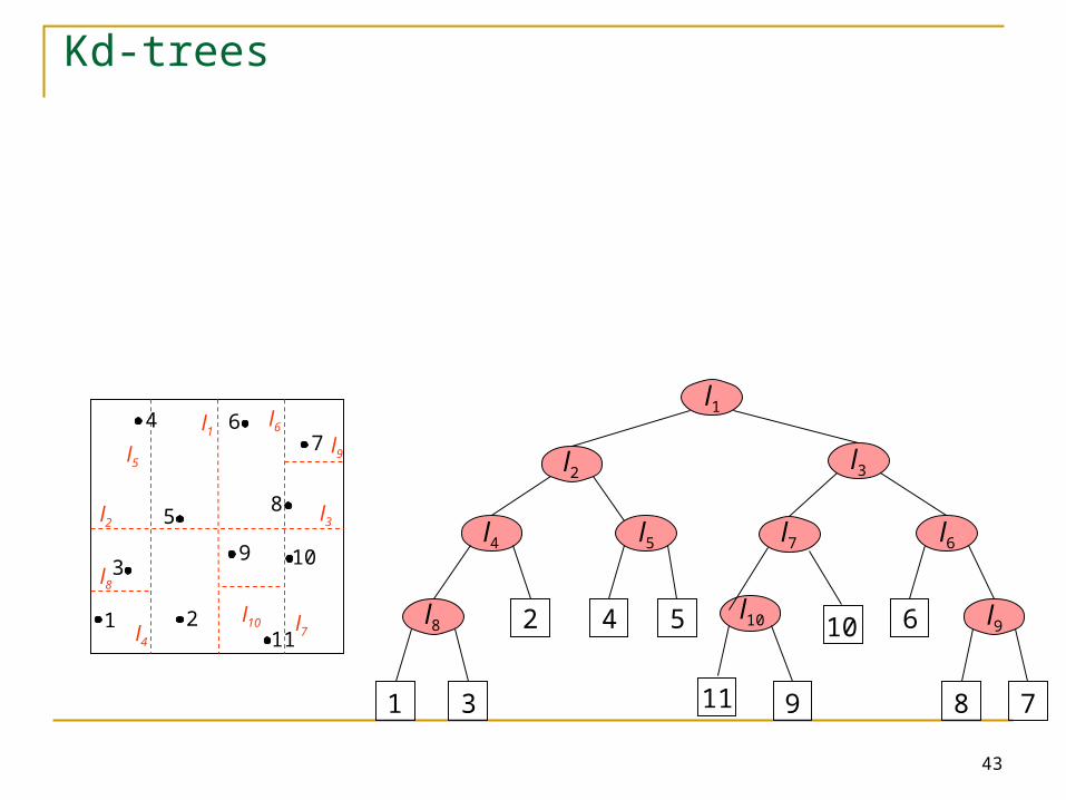
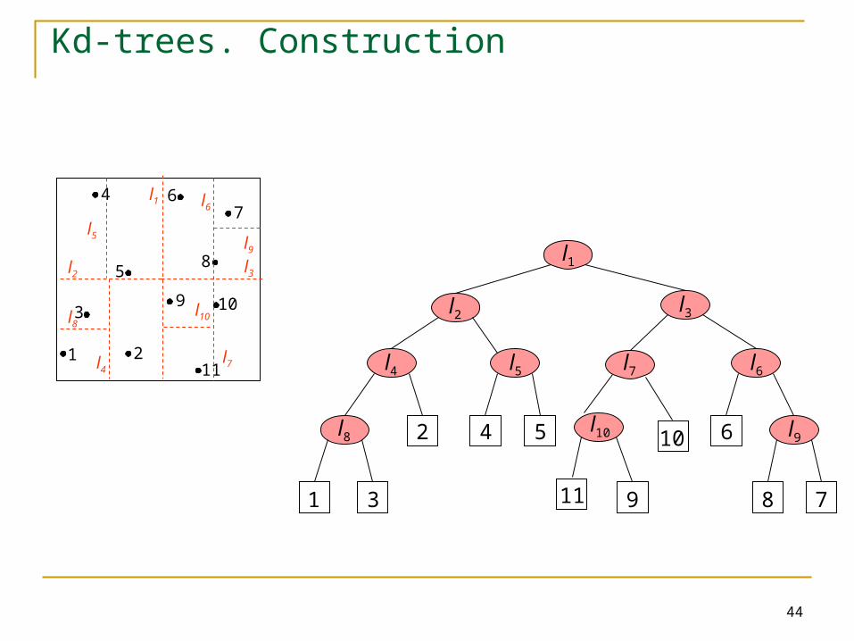
K-d tree K-d tree is a main memory binary tree for

indexing k-dimensional points

The kd-tree is a data structure that is based on recursively subdividing a set of points with alternating axis-aligned hyperplanes.

K-d tree is not necessarily balanced

43

Kd-trees

l1

l8

1

l2l3

l4 l5 l7 l6

l9l10

3

2 4 5

11 9

10 6

8 7

47

6

5

1

3

2

9

8

10

11

l5

l1

l9

l6

l3

l10 l7l4

l8

l2

44

Kd-trees. Construction

47

6

5

1

3

2

9

8

10

11

l5

l1

l9

l6

l3

l10

l7l4

l8

l2

l1

l8

1

l2l3

l4 l5 l7 l6

l9l10

3

2 4 5

11 9

10 6

8 7

45

Z-ordering

Map points from 2-dimensions to 1-dimension. Use a B+-tree to index the 1-dimensional points

Basic assumption: Finite precision in the representation of each co-ordinate, K bits (2K values)

The address space is a square (image) and represented as a 2K x 2K array

46

Z-ordering

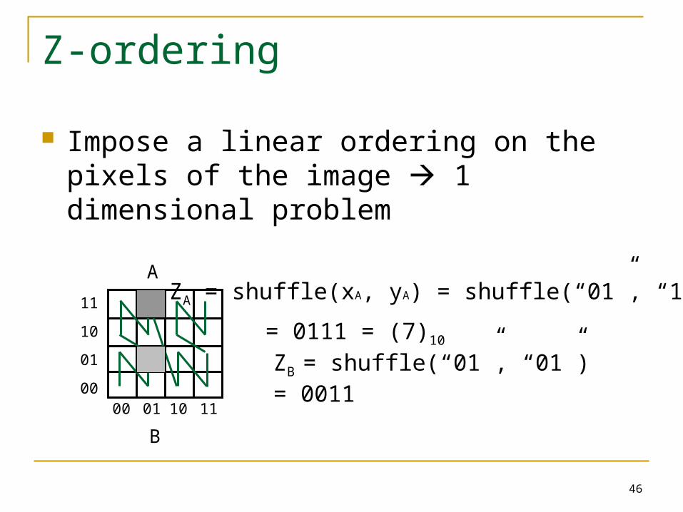
Impose a linear ordering on the pixels of the image 1 dimensional problem

00 01 10 1100

01

10

11

A

B

ZA = shuffle(xA, yA) = shuffle(“01”, “11”)

= 0111 = (7)10

ZB = shuffle(“01”, “01”) = 0011

47

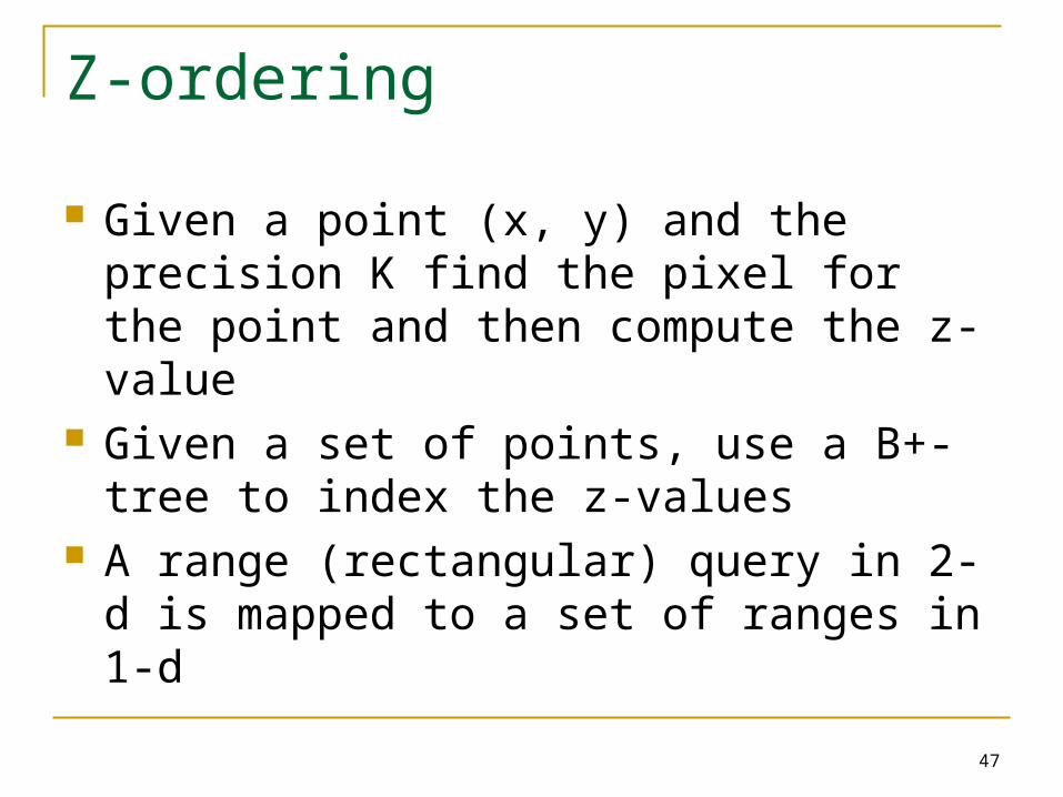
Z-ordering

Given a point (x, y) and the precision K find the pixel for the point and then compute the z-value

Given a set of points, use a B+-tree to index the z-values

A range (rectangular) query in 2-d is mapped to a set of ranges in 1-d

48

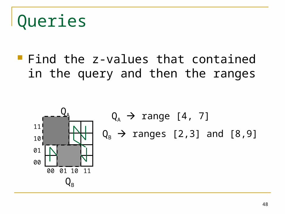
Queries

Find the z-values that contained in the query and then the ranges

00 01 10 1100

01

10

11

QA range [4, 7]QA

QB

QB ranges [2,3] and [8,9]

49

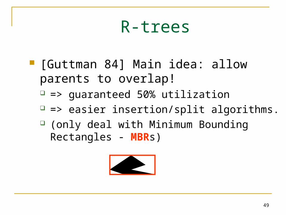
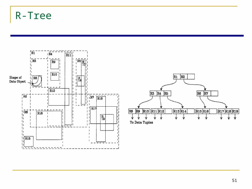
R-trees

[Guttman 84] Main idea: allow parents to overlap! => guaranteed 50% utilization => easier insertion/split algorithms. (only deal with Minimum Bounding Rectangles -

MBRs)

50

R-trees

A multi-way external memory tree Index nodes and data (leaf) nodes All leaf nodes appear on the same level Every node contains between m and M entries The root node has at least 2 entries (children)

51

R-Tree

52

R-Tree

20 4 6 8 10

2

4

6

8

10

x axis

y axis

b

c

a

d

e f

g h

i j

k

l

m

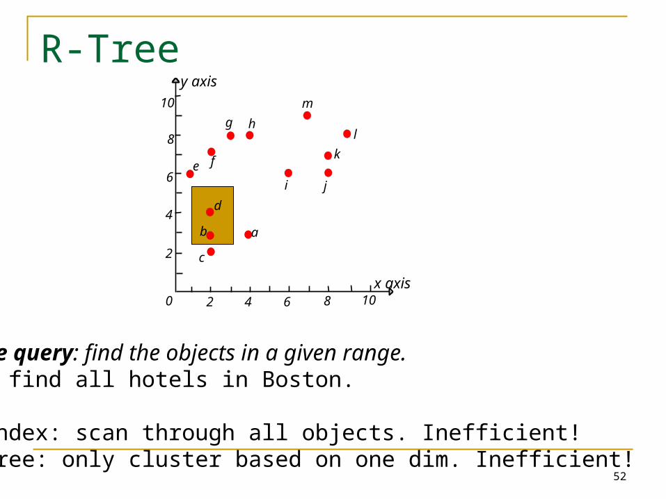
Range query: find the objects in a given range.E.g. find all hotels in Boston.

No index: scan through all objects. Inefficient!B+-tree: only cluster based on one dim. Inefficient!

53

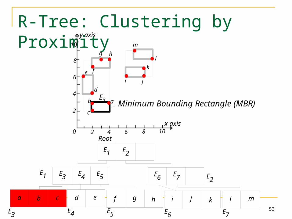
R-Tree: Clustering by Proximity

20 4 6 8 10

2

4

6

8

10

x axis

y axis

b

c

aE3

a b c d e

E1 E2

E3 E4 E5

Root

E1 E2

E3E4

f g h

E5

d

e f

g h

i j

k

l

m

l m

E7

i j k

E6

E6 E7

Minimum Bounding Rectangle (MBR)

54

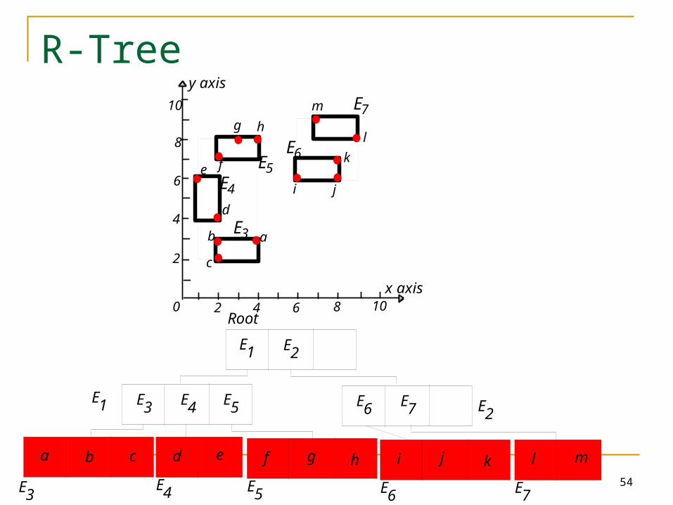
R-Tree

20 4 6 8 10

2

4

6

8

10

x axis

y axis

b

c

aE3

d

e f

g h

i j

k

l

m

E4

E5

E6

E7

a b c d e

E1 E2

E3 E4 E5

Root

E1 E2

E3E4

f g h

E5

l m

E7

i j k

E6

E6 E7

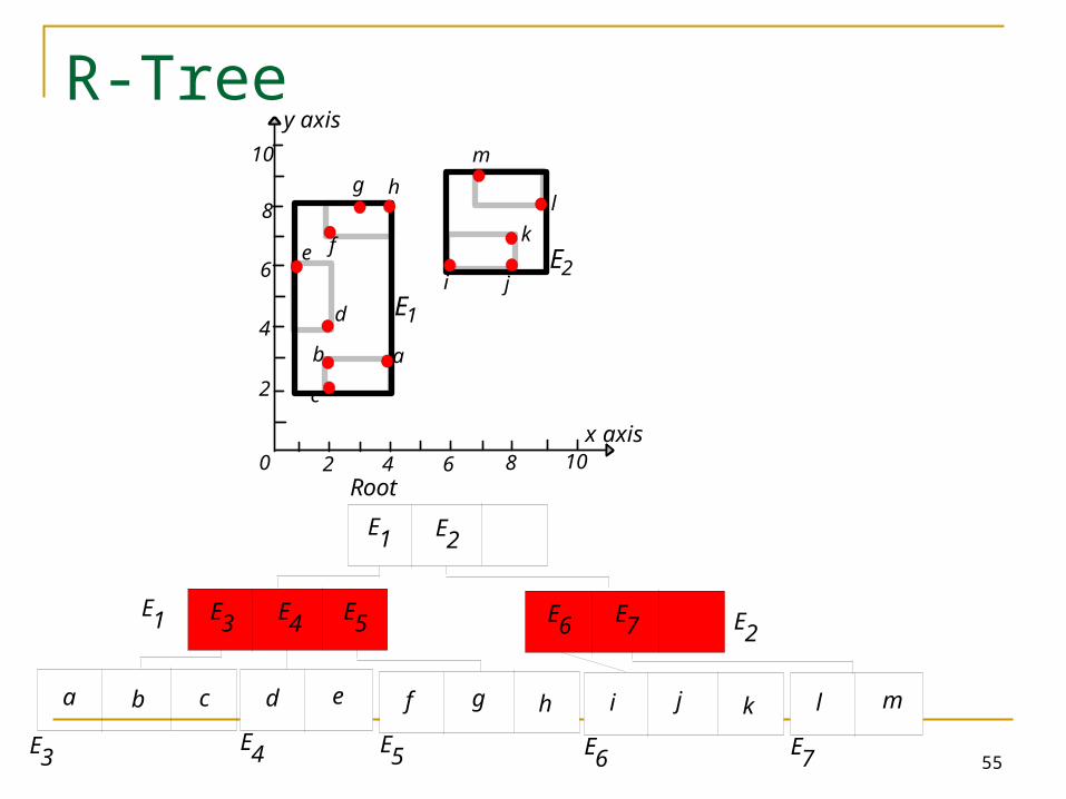
55

R-Tree

20 4 6 8 10

2

4

6

8

10

x axis

y axis

b

c

a

E1d

e f

g h

i j

k

l

m

E2

a b c d e

E1 E2

E3 E4 E5

Root

E1 E2

E3E4

f g h

E5

l m

E7

i j k

E6

E6 E7

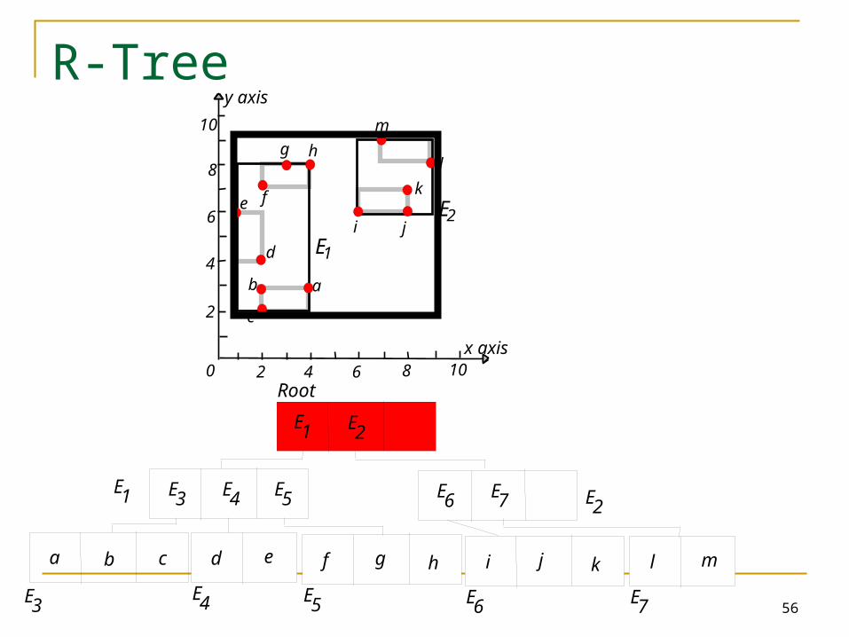
56

R-Tree

20 4 6 8 10

2

4

6

8

10

x axis

y axis

b

c

a

E1d

e f

g h

i j

k

l

m

E2

a b c d e

E1 E2

E3 E4 E5

Root

E1 E2

E3E4

f g h

E5

l m

E7

i j k

E6

E6 E7

57

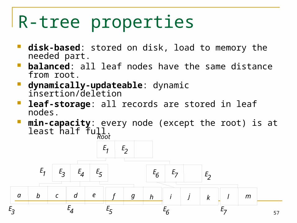
R-tree properties

a b c d e

E1 E2

E3 E4 E5

Root

E1 E2

E3E4

f g h

E5

l m

E7

i j k

E6

E6 E7

disk-based: stored on disk, load to memory the needed part. balanced: all leaf nodes have the same distance from root. dynamically-updateable: dynamic insertion/deletion leaf-storage: all records are stored in leaf nodes. min-capacity: every node (except the root) is at least half full.

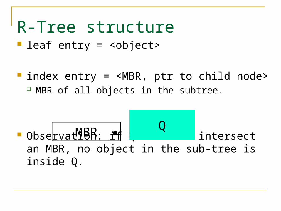
R-Tree structure leaf entry = <object>

index entry = <MBR, ptr to child node> MBR of all objects in the subtree.

Observation: if Q does not intersect an MBR, no object in the sub-tree is inside Q.

QMBR

59

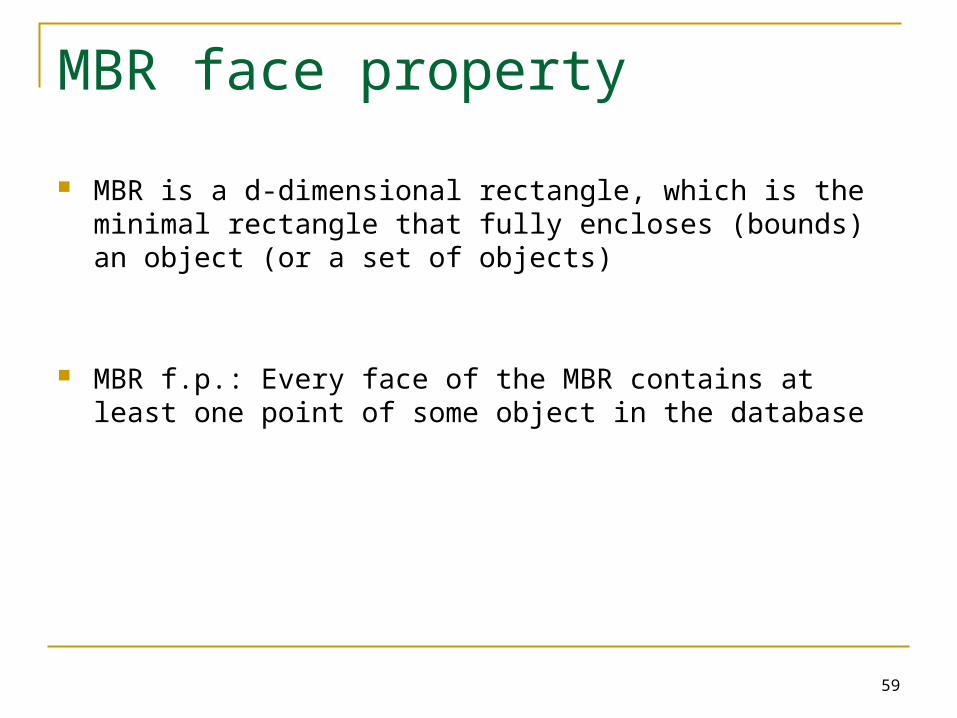
MBR face property

MBR is a d-dimensional rectangle, which is the minimal rectangle that fully encloses (bounds) an object (or a set of objects)

MBR f.p.: Every face of the MBR contains at least one point of some object in the database

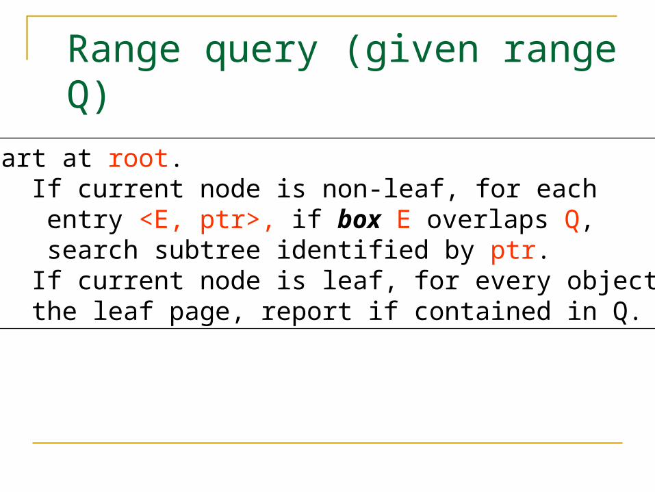
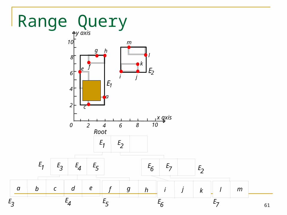
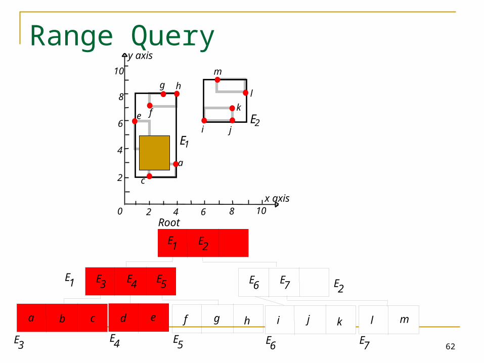
Range query (given range Q)

Start at root.1. If current node is non-leaf, for each entry <E, ptr>, if box E overlaps Q, search subtree identified by ptr.2. If current node is leaf, for every object in the leaf page, report if contained in Q.

61

Range Query

20 4 6 8 10

2

4

6

8

10

x axis

y axis

b

c

a

E1d

e f

g h

i j

k

l

m

E2

a b c d e

E1 E2

E3 E4 E5

Root

E1 E2

E3E4

f g h

E5

l m

E7

i j k

E6

E6 E7

62

Range Query

20 4 6 8 10

2

4

6

8

10

x axis

y axis

b

c

a

E1d

e f

g h

i j

k

l

m

E2

a b c d e

E1 E2

E3 E4 E5

Root

E1 E2

E3E4

f g h

E5

l m

E7

i j k

E6

E6 E7

63

KNN Search in a R tree

Visit an MBR (node) only when necessary

How to do pruning? Using MINDIST and MINMAXDIST

64

MINDIST

MINDIST(P, R) is the minimum distance between a point P and a rectangle R

If the point is inside R, then MINDIST=0 If P is outside of R, MINDIST is the distance of P to the closest

point of R (one point of the perimeter)

65

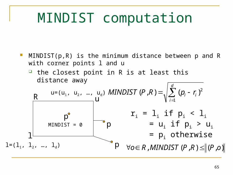
MINDIST computation

MINDIST(p,R) is the minimum distance between p and R with corner points l and u the closest point in R is at least this distance away

ri = li if pi < li

= ui if pi > ui

= pi otherwise

pp

p

R

l

u

MINDIST = 0

d

iii rpRPMINDIST

1

2)(),(

l=(l1, l2, …, ld)

u=(u1, u2, …, ud)

),(),(, oPRPMINDISTRo

66

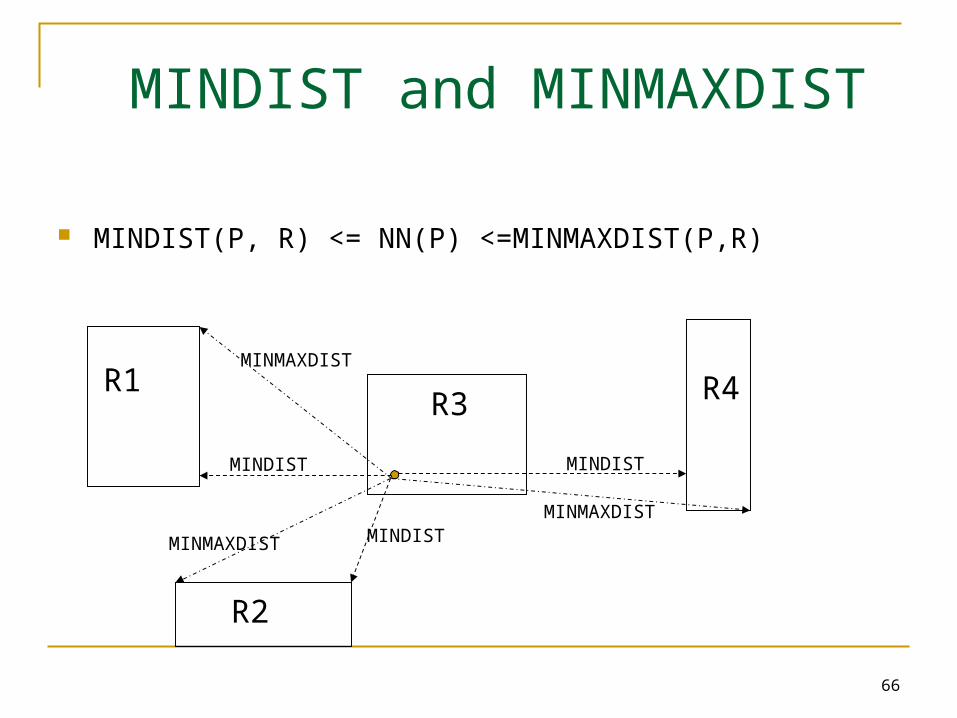
MINDIST and MINMAXDIST

MINDIST(P, R) <= NN(P) <=MINMAXDIST(P,R)

R1

R2

R3 R4

MINDIST

MINMAXDIST

MINDISTMINMAXDIST

MINMAXDIST

MINDIST

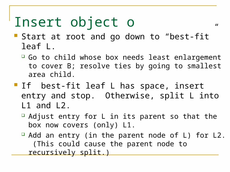
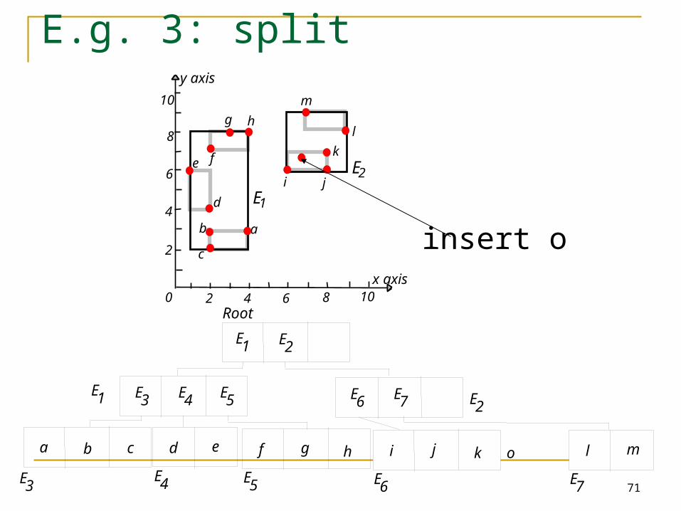
Insert object o Start at root and go down to “best-fit” leaf L.

Go to child whose box needs least enlargement to cover B; resolve ties by going to smallest area child.

If best-fit leaf L has space, insert entry and stop. Otherwise, split L into L1 and L2. Adjust entry for L in its parent so that the box now

covers (only) L1. Add an entry (in the parent node of L) for L2. (This

could cause the parent node to recursively split.)

68

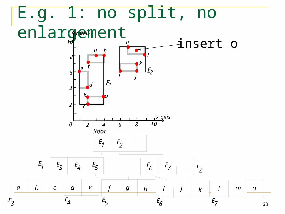
E.g. 1: no split, no enlargement

20 4 6 8 10

2

4

6

8

10

x axis

y axis

b

c

a

E1d

e f

g h

i j

k

l

m

E2

a b c d e

E1 E2

E3 E4 E5

Root

E1 E2

E3E4

f g h

E5

l m

E7

i j k

E6

E6 E7

insert o

o

69

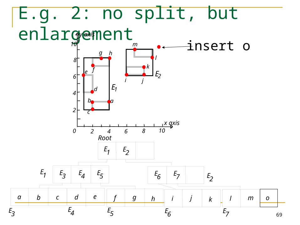
E.g. 2: no split, but enlargement

20 4 6 8 10

2

4

6

8

10

x axis

y axis

b

c

a

E1d

e f

g h

i j

k

l

m

E2

a b c d e

E1 E2

E3 E4 E5

Root

E1 E2

E3E4

f g h

E5

l m

E7

i j k

E6

E6 E7

insert o

o

70

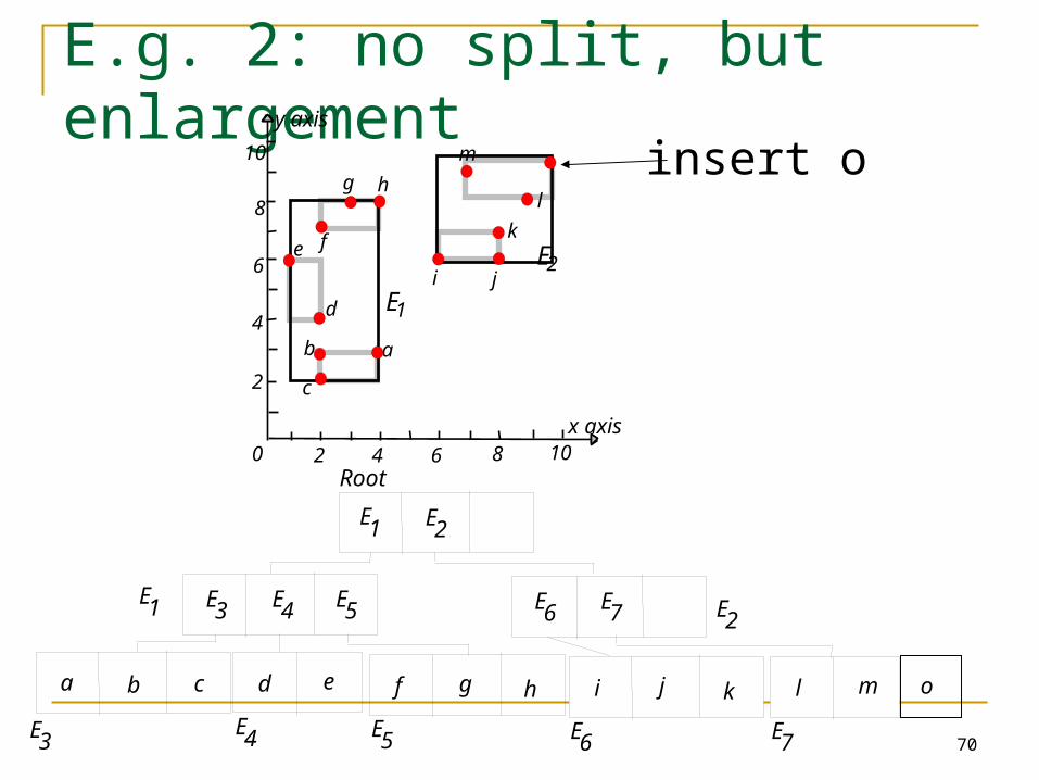
E.g. 2: no split, but enlargement

20 4 6 8 10

2

4

6

8

10

x axis

y axis

b

c

a

E1d

e f

g h

i j

k

l

m

E2

a b c d e

E1 E2

E3 E4 E5

Root

E1 E2

E3E4

f g h

E5

l m

E7

i j k

E6

E6 E7

insert o

o

71

E.g. 3: split

20 4 6 8 10

2

4

6

8

10

x axis

y axis

b

c

a

E1d

e f

g h

i j

k

l

m

E2

a b c d e

E1 E2

E3 E4 E5

Root

E1 E2

E3E4

f g h

E5

l m

E7

i j k

E6

E6 E7

insert o

o

72

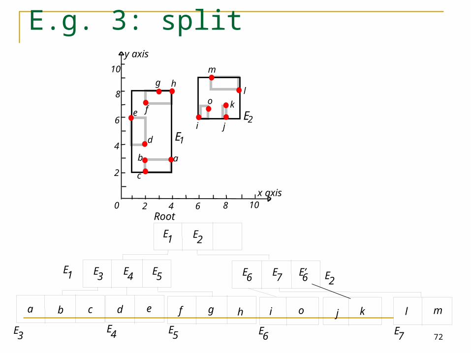
E.g. 3: split

20 4 6 8 10

2

4

6

8

10

x axis

y axis

b

c

a

E1d

e f

g h

i j

k

l

m

E2

a b c d e

E1 E2

E3 E4 E5

Root

E1 E2

E3E4

f g h

E5

l m

E7

i o j

E6

E6 E7

k

o

E’6

73

R-trees: Variations

R+-tree: DO not allow overlapping, so split the objects (similar to z-values)

R*-tree: change the insertion, deletion algorithms (minimize not only area but also perimeter, forced re-insertion )

74

Spatio-Temporal Databases

75

Introduction

Spatio-temporal Databases: manage spatial data whose geometry changes over time

Geometry: position and/or extent Global change data: climate or land cover changes Transportation: cars, airplanes Animated movies/video DBs

76

ST DBs

A special Temporal Database All the features of temporal database Attributes can be spatial also

Extension of Spatial Databases Objects change instead of being static At any timestamp it is a conventional Spatial

Database New Database type

77

Requirements

Efficient Representation of Space and Time Data Models Query Languages Query processing and Indexing GUI for spatio-temporal datasets

78

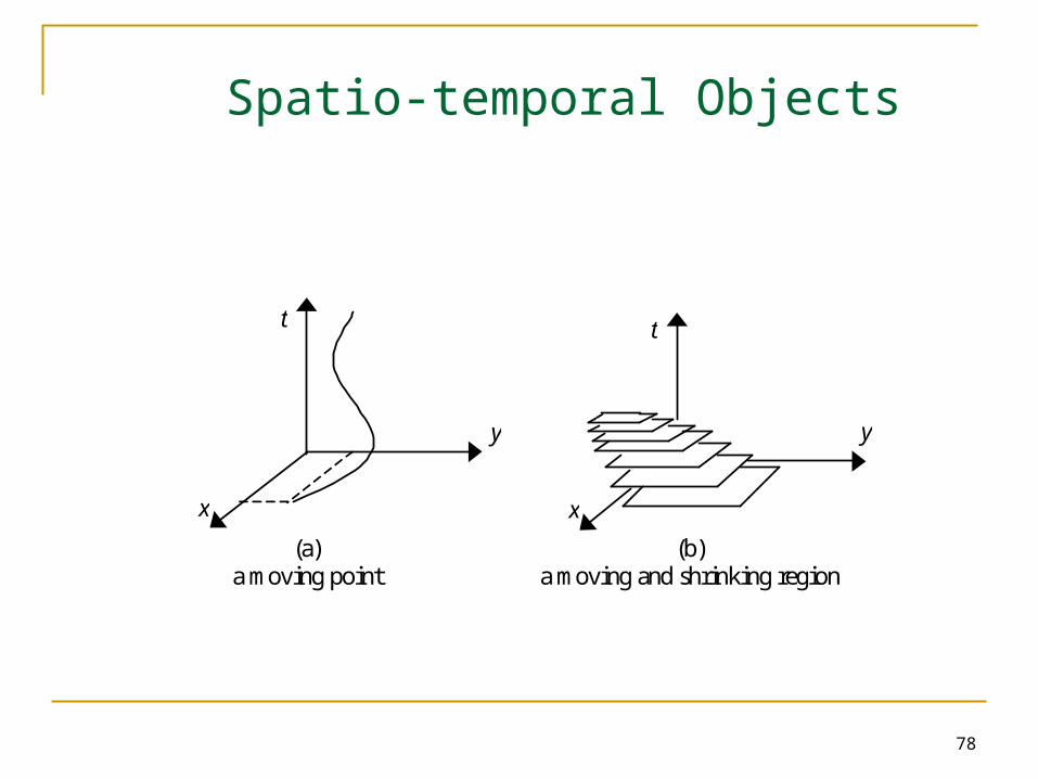
Spatio-temporal Objects

(a) (b) a moving point a moving and shrinking region

y

t

x

y

t

x

79

ST Queries

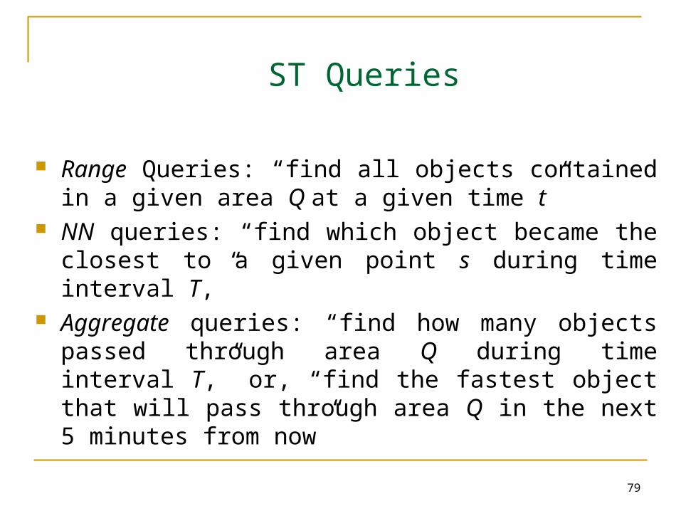
Range Queries: “find all objects contained in a given area Q at a given time t”

NN queries: “find which object became the closest to a given point s during time interval T,”

Aggregate queries: “find how many objects passed through area Q during time interval T,” or, “find the fastest object that will pass through area Q in the next 5 minutes from now”

80

ST Queries

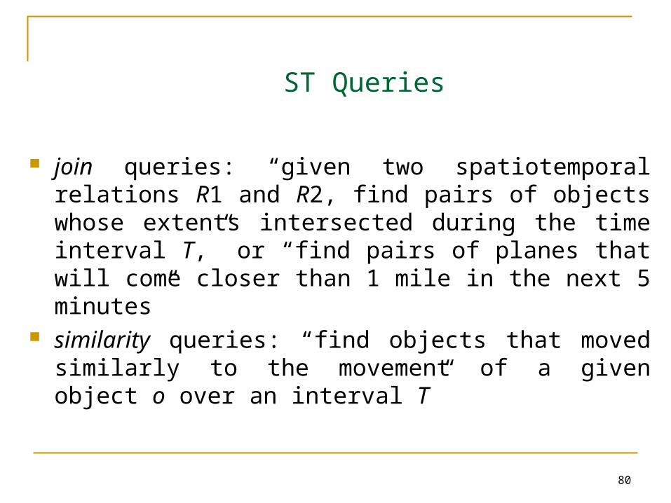
join queries: “given two spatiotemporal relations R1 and R2, find pairs of objects whose extents intersected during the time interval T,” or “find pairs of planes that will come closer than 1 mile in the next 5 minutes”

similarity queries: “find objects that moved similarly to the movement of a given object o over an interval T”

81

SP Data Types

Moving Points Extent does not matter Each object is modeled as a point (moving vehicles in a

GIS based transportation system) Moving regions

Extent matters! Each object is represented by an MBR, the MBR can

change as the object move (airplanes, storm,…)

82

SP Data Types

Different Type of changes: Changes are applied discretely

Urban planning: appearance or dis-appearance of buildings

Changes are applied continuously Moving objects (eg. Vehicles)

83

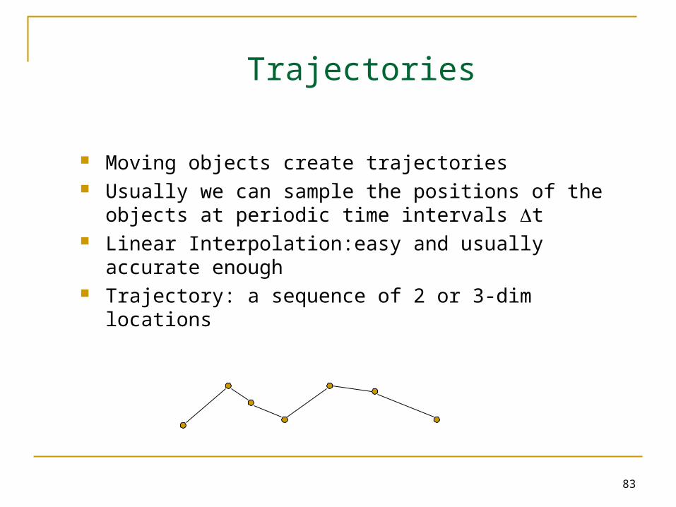
Trajectories

Moving objects create trajectories Usually we can sample the positions of the objects at

periodic time intervals t Linear Interpolation:easy and usually accurate enough Trajectory: a sequence of 2 or 3-dim locations

84

Temporal Environment

Valid time Two types of environments:

Predicting the future positions: Each object has a velocity vector. The DB can predict the location at any time t>tnow assuming linear movement. Queries refer to the future

Storing the history. Queries refer to the past states of the spatial database

85

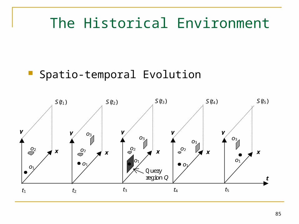
The Historical Environment

Spatio-temporal Evolution

x x x x x

t

t1 t5t4t3t2

S(t1) S(t5)S(t4)S(t3)S(t2)

y y y y y

o2 o2o2 o2

o3 o3 o3o3

o1o1 o1

o1o1

Queryregion Q

86

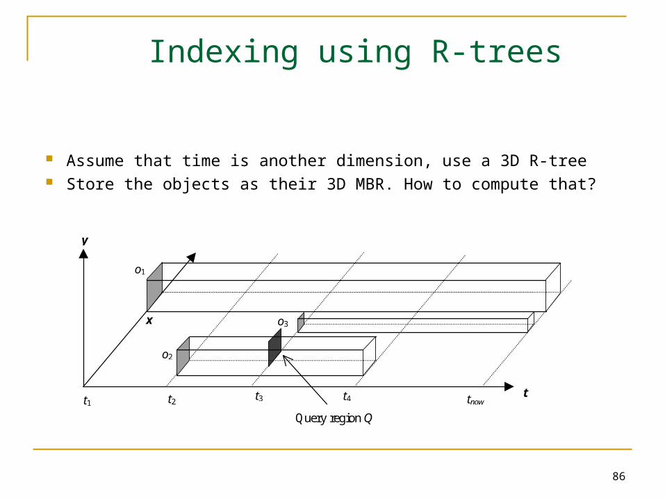
Indexing using R-trees

Assume that time is another dimension, use a 3D R-tree Store the objects as their 3D MBR. How to compute that?

x

tt1

t3t2

y

o2

o3

Query region Q

o1

t4 tnow

87

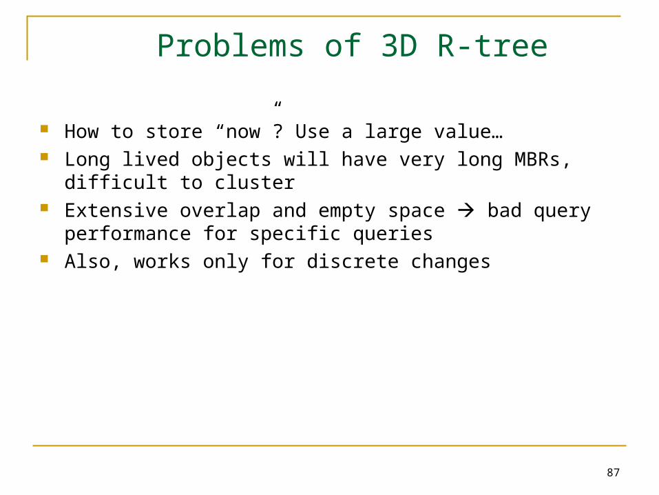
Problems of 3D R-tree

How to store “now”? Use a large value… Long lived objects will have very long MBRs, difficult to cluster Extensive overlap and empty space bad query performance

for specific queries Also, works only for discrete changes

88

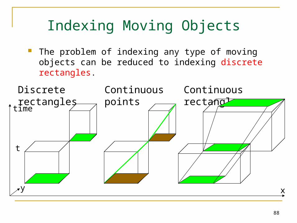
Indexing Moving Objects

The problem of indexing any type of moving objects can be reduced to indexing discrete rectangles.

Continuous points Continuous rectanglesDiscrete rectangles

xy

time

t

89

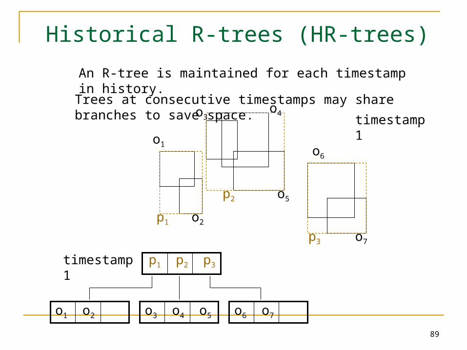
Historical R-trees (HR-trees)

o1

o2

o6

o7

o5

p1 p2 p3

o1 o2 o3 o4 o5 o6 o7

p1

p2

p3

o4o3

timestamp 1

timestamp 1

An R-tree is maintained for each timestamp in history.

Trees at consecutive timestamps may share branches to save space.

90

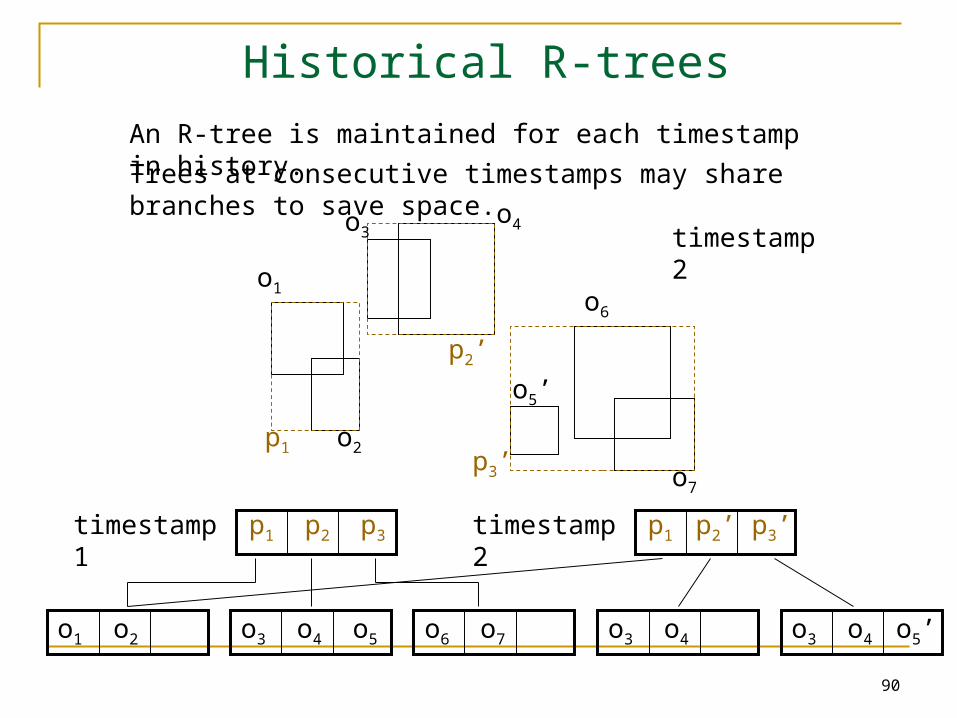
Historical R-treesAn R-tree is maintained for each timestamp in history.

Trees at consecutive timestamps may share branches to save space.

p1 p2 p3

o1 o2 o3 o4 o5 o6 o7

timestamp 1 p1 p2’ p3’

o3 o4

timestamp 2

o3 o4 o5’

o1

o2

o6

o7

o5’

p1

p2’

p3’

o4o3 timestamp 2

91

HR-trees: Pros and Cons

• HR-trees answer timestamp queries very efficiently.

– A timestamp query degenerates into a spatial window query handled by the corresponding R-tree at the query timestamp.

• Not quite efficient:

– Expensive space consumption.

A node needs to be duplicated even when only one object moves.

– Interval query processing is inefficient.

Although redundancy (from duplication) is necessary to maintain good timestamp query performance, it is excessive in HR-trees.