Embed Size (px)
Citation preview
Intel and MobileODT Cervical Cancer Screening Kaggle Competition:Cervix Type Classification Using Deep Learning and Image Classification
Jack PayetteStanford University
Jake RachleffStanford University
Cameron Van de GraafStanford [email protected]
Abstract
In this project, we attempted to create a deep learningmodel to classify cervix types in order to help health-care providers provide better care to women all overthe world. The problem is specified by the KaggleChallenge found at https://www.kaggle.com/c/intel-mobileodt-cervical-cancer-screening.Classification of medical images is known to be a difficultproblem for a number of reasons, but recent advancementsin Deep Learning techniques have shown promise for suchtasks. We experimented with a number of convolutionalarchitectures before settling on residual neural networkswith dropout and batch normalization to produces scoresfor each class, with loss calculated based on the multi-classlogarithmic loss. The dataset, which was provided byKaggle, consists of 1481 training images, 512 test images,and 4633 additional images that we used for training. Dueto the small nature of the dataset, we used a number of dataaugmentation techniques. Through experimentation, wefound that it is indeed very difficult for train a model fromscratch that is general enough to solve this problem. Whilemany techniques gave us marginal improvements in ourperformance, we were unable to reach a truly competitivespot on the leaderboard, likely as a result of overfittingsuch a limited dataset.
1. Introduction
Cervical cancer is a deadly but highly treatable disease aslong as it’s detected in early stages and the correct treatmentis administered. Healthcare specialists have broken cervixesdown into three types. Women with Type 1 cervixes donot require screening beyond the standard procedure, whilewomen with Type 2 and Type 3 cervixes require more time-consuming screening processes. Many healthcare providersin low resource areas of the world have neither the timenor the expertise to make cervix type classifications, sowomen all over the world are missing out on potentially
lifesaving cancer screenings. For our project, we haveentered the Kaggle competition hosted by Intel and Mo-bileODT (found at https://www.kaggle.com/c/intel-mobileodt-cervical-cancer-screening)to create an image classifier for different cervix types. Theinput to our classifier is a medical image of a cervix, andwe use deep residual CNNs to output the probability ofthe cervix being in each of the three classes. Our hope isthat we can create a system that can aid doctors around theworld in classifying cervix type and in turn help womenget the cervical cancer screening that could potentially savetheir lives.
2. Related WorksGeneral Deep Learning Background
We saw the relevant body of literature for this work asbeing divided between three rather distinct subject areas.Firstly, we relied heavily on general literature pertaining totopics we had exposure to in this class - CNNs, dropout,batch normalization, etc. We mostly referenced papers thatwere suggested to us over the course of the class, Bengio’spaper on dropout being a prime example. We would alsoput several of the external codebases into this section, in-cluding Tensorflow and associated documentation as wellas the imgaug library. However, we leave most of the de-tailed explication of how these works influenced our ownfor the subsequent sections on data and methods.
Deep Learning in Medical Imaging Tasks
The second category of background literature is that per-taining to the application of deep learning in medical imageclassification, segmentation, etc. For this section, we be-gan with a fairly comprehensive review by Litjens et. alfrom February 2017 - supplemented by more specific read-ings in areas of interest. One of the high-level findings wasthat the use of CNNs and other deep learning architecturesin medical imaging tasks has exploded over the past sev-eral years, from a negligible number of papers publishedin the field during 2014, to around 50 in 2015, and reach-
1
ing around 500 in 2016. Classification for exam purposes,of the type we are attempting to accomplish here, was thethird most common task addressed across all papers. How-ever, we saw few papers that attempted classification of nor-mal photographic images, with the vast majority of pub-lications focusing on the common investigative modalitiesof MRI, microscopy, and CT. In terms of CNN architec-tures commonly applied to medical tasks, ResNet, VGG,and Inception were the most commonly utilized frameworks(Liu 2016). Transfer learning has often been applied, giventhe frequently limited quantities of labeled data available,though results are mixed between fine-tuning and featureextraction approaches (Antony 2016). More recent papershave achieved better results training models from scratch ondatasets of >1000 images (Menegola 2016).
A particularly important point discussed in multiple pa-pers was that it is often elements such as image augmen-tation and pre-processing that made the ultimate differ-ence in performance more than simply adding more layers.Such domain-specific alterations can improve performanceas much as 10%, and can be as specific as stain normaliza-tion and as general as elastic transformations (Ronneberger2015). Though we couldn’t find much evidence of CNNs orother deep learning architectures being applied to cervix im-ages, the closest analogue we could find was classificationof dermatological conditions by standard photographic im-ages, where authors were able to achieve human-level per-formance using Inception-v3 (Esteva 2017).
There is also a substantial literature devoted to the uniqueproblems faced in applying deep learning to medical imag-ing, many of which we encountered over the course ofour project. For instance, many papers cite the dangersof falsely labeled images or poor quality data, which in-fluenced our approach to image curation and removal (Ar-mato 2011). Class imbalance - oftentimes resulting fromthe relative rarity of physiological types or medical condi-tions in the general population - is another issue that can beseverely detrimental to system performance; this has beenaddressed through rebalancing and augmentation specifi-cally applied to minority classes (Pereira 2016). It is alsodifficult to discern whether a classification paradigm is al-ways the optimal approach as contrasted with a segmenta-tion or predicted bounding box approach (Sirinukunwattanaet al. 2016). Generally Litjens et. al were optimistic aboutapplications of deep learning in medical imaging, with theaforementioned caveats.
Approaches to Cervix Segmentation
While deep learning models have not (so far as we know)been applied to the problem of cervix classification and seg-mentation prior to the launch of this Kaggle competition,there is some literature describing other statistical methodsfor accomplishing these tasks. The first paper we could find
on this topic was by Gordon and Zimmerman from 2004,which introduced a segmentation paradigm based on statis-tical properties of the texture and color profile of differentparts of cervix images (Gordon 2004). This work was ex-tended slightly by Srinivasan et al. in 2005, where similartechniques were applied to cervix cancer detection specifi-cally. Finally in 2010 Xue et al. developed the most fullyfledged suite of cervix analysis tools for detection, segmen-tation, and classification (Xue 2010). Unfortunately, thistoolset was implemented using Java applets more suited tothe clinical environment where smaller volumes of imageswere being processed. With this in mind, we adapted codewritten by Kaggle user Chattob (link to code in references)that implements the algorithms in the above papers to gen-erate cropping circles and bounding boxes. Chattob’s codein turn was based on a follow up to the 2004 Gordon paper(Greenspan 2009).
3. Datasets and FeaturesThe dataset that we used for this project was the one pro-
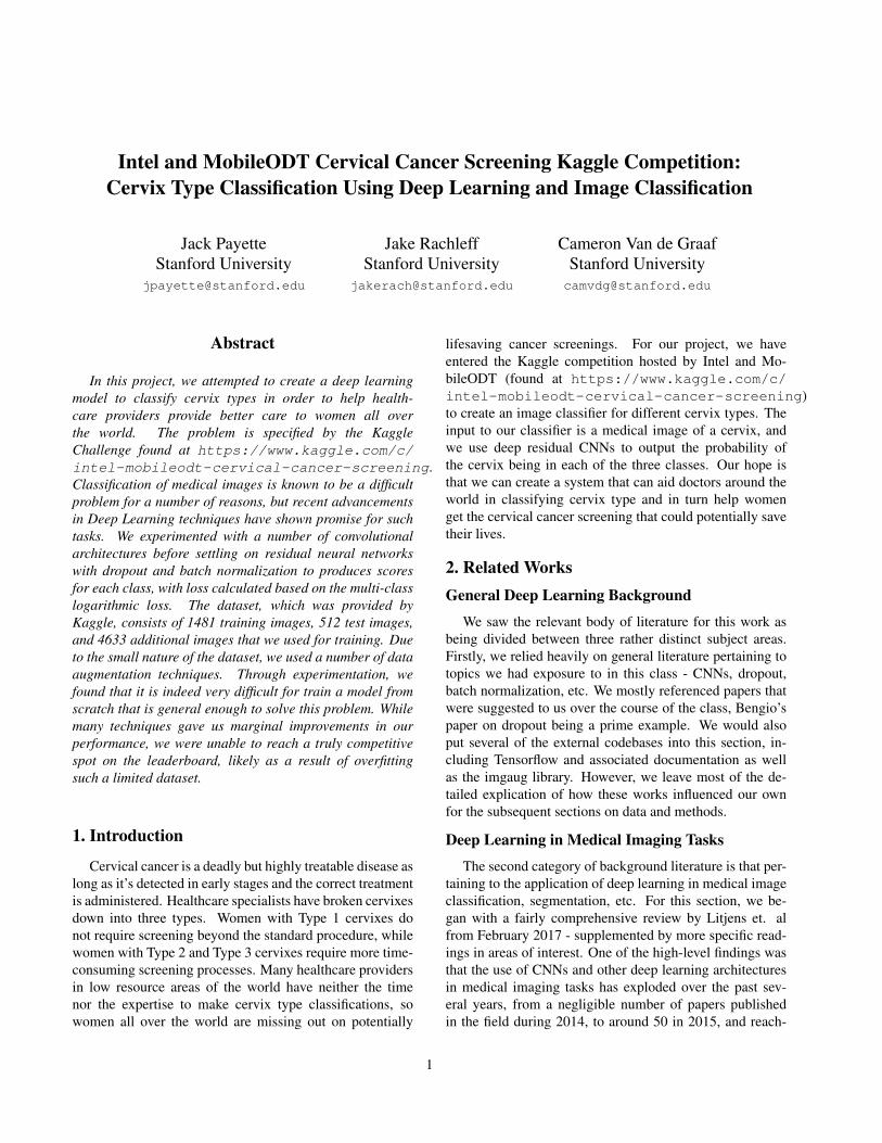
vided by Kaggle for this competition. A breakdown of thedataset can be seen in Figure 1.
Figure 1. A breakdown of the Kaggle datatset
To generate our Validation split, we used 50% of theTrain images for our Training Set and 50% of our Train-ing images for our Validation Set. We used the additionaldata as part of our Training Set as well. The reasoning forsplitting our data like this is that the Train data consists ofhigh quality images, all from different patients, with no du-plicates. The additional data, on the other hand, consistsof lower quality images, many of which come from thesame patients, and most importantly, contains duplicates.For this reason, we did not use any of the additional imagesin our validation set, as this would create the possibility ofa duplicate image being in both the Training and ValidationSet. This would artificially increase the performance of ourmodel on the Validation Set, meaning that the Validation Setwould no longer serve as a good proxy for the Test Set.
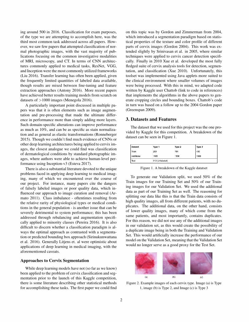
Figure 2. Example images of each cervix type. Image (a) is Type1, image (b) is Type 2, and Image (c) is Type 3
2
The sizes of the images in this dataset vary greatly, fromas small as 480 x 640 to as large as 3096 x 4128. As a re-sult, we used image resizing techniques so that all of ourdata was 224 x 224 by the time the model received it as in-put. On the training images, we resized the image so thatthe shortest side was 256 pixels, and then took a random224 x 224 crop. This is a common technique for data aug-mentation. For validation and test images, we resized themso that the side was 224 pixels, and we took the crop fromthe center of the other axis. We chose this exact algorithmbecause there are images in both landscape and portrait for-mat. As suggested by TA Ben Poole, we did not subtractthe mean image from each image, as this is not consideredbest practice for medical imaging. We did, however, divideevery pixel value by 255 so that every pixel value was in therange of 0 to 1.
Due to the limited nature of our dataset, we employed anumber of different data augmentation techniques. The firstwas that we upsampled from the underrepresented classesso that the data distribution was even among all of theclasses. While we believe that this is the “correct” way totrain this classifier, we noticed that our models performedworse when we did this. We believe that this is because theunderlying distribution of the test set more closely matchesthat of the training set, rather than that of an even distribu-tion.
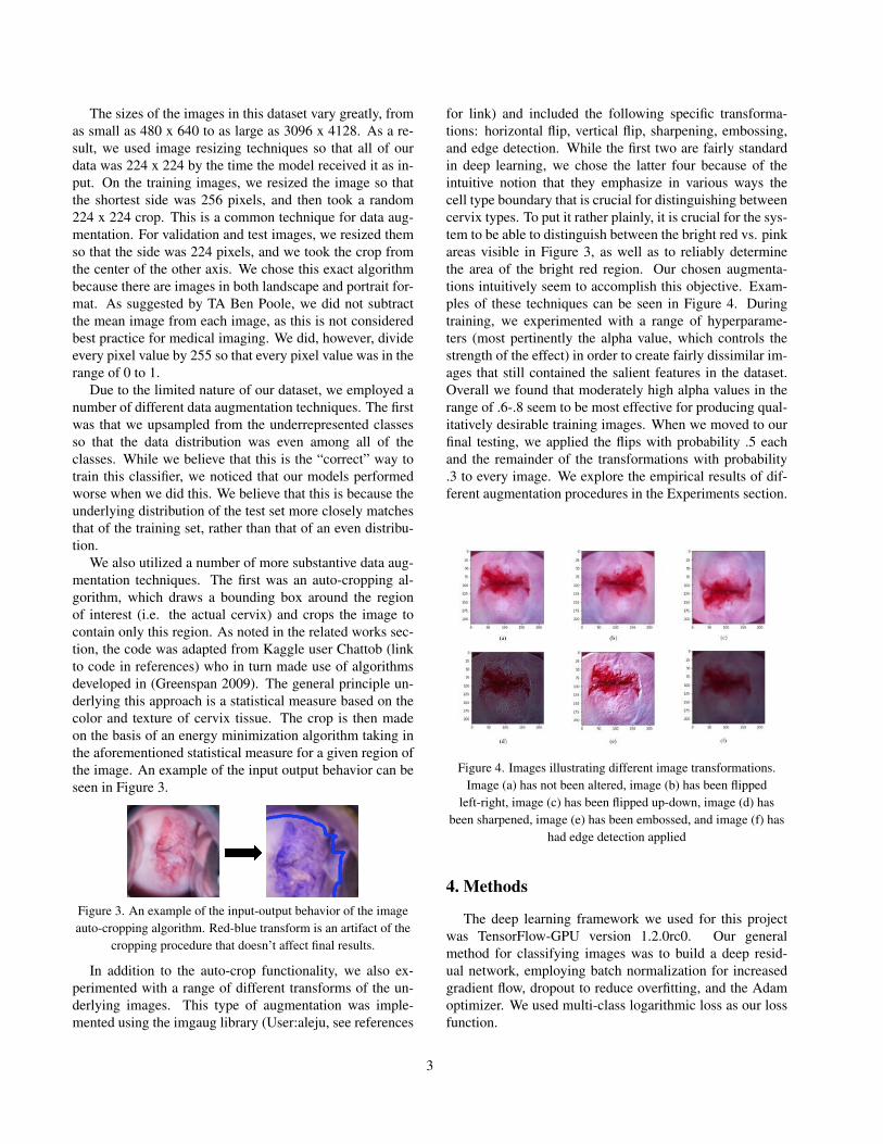
We also utilized a number of more substantive data aug-mentation techniques. The first was an auto-cropping al-gorithm, which draws a bounding box around the regionof interest (i.e. the actual cervix) and crops the image tocontain only this region. As noted in the related works sec-tion, the code was adapted from Kaggle user Chattob (linkto code in references) who in turn made use of algorithmsdeveloped in (Greenspan 2009). The general principle un-derlying this approach is a statistical measure based on thecolor and texture of cervix tissue. The crop is then madeon the basis of an energy minimization algorithm taking inthe aforementioned statistical measure for a given region ofthe image. An example of the input output behavior can beseen in Figure 3.
Figure 3. An example of the input-output behavior of the imageauto-cropping algorithm. Red-blue transform is an artifact of the
cropping procedure that doesn’t affect final results.
In addition to the auto-crop functionality, we also ex-perimented with a range of different transforms of the un-derlying images. This type of augmentation was imple-mented using the imgaug library (User:aleju, see references
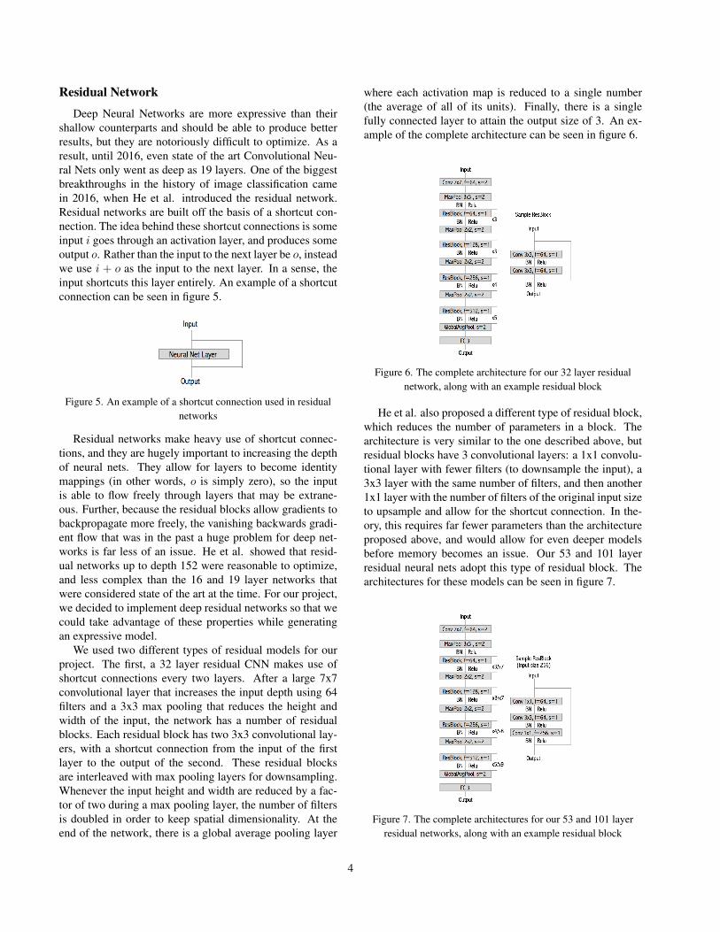
for link) and included the following specific transforma-tions: horizontal flip, vertical flip, sharpening, embossing,and edge detection. While the first two are fairly standardin deep learning, we chose the latter four because of theintuitive notion that they emphasize in various ways thecell type boundary that is crucial for distinguishing betweencervix types. To put it rather plainly, it is crucial for the sys-tem to be able to distinguish between the bright red vs. pinkareas visible in Figure 3, as well as to reliably determinethe area of the bright red region. Our chosen augmenta-tions intuitively seem to accomplish this objective. Exam-ples of these techniques can be seen in Figure 4. Duringtraining, we experimented with a range of hyperparame-ters (most pertinently the alpha value, which controls thestrength of the effect) in order to create fairly dissimilar im-ages that still contained the salient features in the dataset.Overall we found that moderately high alpha values in therange of .6-.8 seem to be most effective for producing qual-itatively desirable training images. When we moved to ourfinal testing, we applied the flips with probability .5 eachand the remainder of the transformations with probability.3 to every image. We explore the empirical results of dif-ferent augmentation procedures in the Experiments section.
Figure 4. Images illustrating different image transformations.Image (a) has not been altered, image (b) has been flipped
left-right, image (c) has been flipped up-down, image (d) hasbeen sharpened, image (e) has been embossed, and image (f) has
had edge detection applied
4. Methods
The deep learning framework we used for this projectwas TensorFlow-GPU version 1.2.0rc0. Our generalmethod for classifying images was to build a deep resid-ual network, employing batch normalization for increasedgradient flow, dropout to reduce overfitting, and the Adamoptimizer. We used multi-class logarithmic loss as our lossfunction.
3
Residual Network
Deep Neural Networks are more expressive than theirshallow counterparts and should be able to produce betterresults, but they are notoriously difficult to optimize. As aresult, until 2016, even state of the art Convolutional Neu-ral Nets only went as deep as 19 layers. One of the biggestbreakthroughs in the history of image classification camein 2016, when He et al. introduced the residual network.Residual networks are built off the basis of a shortcut con-nection. The idea behind these shortcut connections is someinput i goes through an activation layer, and produces someoutput o. Rather than the input to the next layer be o, insteadwe use i + o as the input to the next layer. In a sense, theinput shortcuts this layer entirely. An example of a shortcutconnection can be seen in figure 5.
Figure 5. An example of a shortcut connection used in residualnetworks
Residual networks make heavy use of shortcut connec-tions, and they are hugely important to increasing the depthof neural nets. They allow for layers to become identitymappings (in other words, o is simply zero), so the inputis able to flow freely through layers that may be extrane-ous. Further, because the residual blocks allow gradients tobackpropagate more freely, the vanishing backwards gradi-ent flow that was in the past a huge problem for deep net-works is far less of an issue. He et al. showed that resid-ual networks up to depth 152 were reasonable to optimize,and less complex than the 16 and 19 layer networks thatwere considered state of the art at the time. For our project,we decided to implement deep residual networks so that wecould take advantage of these properties while generatingan expressive model.
We used two different types of residual models for ourproject. The first, a 32 layer residual CNN makes use ofshortcut connections every two layers. After a large 7x7convolutional layer that increases the input depth using 64filters and a 3x3 max pooling that reduces the height andwidth of the input, the network has a number of residualblocks. Each residual block has two 3x3 convolutional lay-ers, with a shortcut connection from the input of the firstlayer to the output of the second. These residual blocksare interleaved with max pooling layers for downsampling.Whenever the input height and width are reduced by a fac-tor of two during a max pooling layer, the number of filtersis doubled in order to keep spatial dimensionality. At theend of the network, there is a global average pooling layer
where each activation map is reduced to a single number(the average of all of its units). Finally, there is a singlefully connected layer to attain the output size of 3. An ex-ample of the complete architecture can be seen in figure 6.
Figure 6. The complete architecture for our 32 layer residualnetwork, along with an example residual block
He et al. also proposed a different type of residual block,which reduces the number of parameters in a block. Thearchitecture is very similar to the one described above, butresidual blocks have 3 convolutional layers: a 1x1 convolu-tional layer with fewer filters (to downsample the input), a3x3 layer with the same number of filters, and then another1x1 layer with the number of filters of the original input sizeto upsample and allow for the shortcut connection. In the-ory, this requires far fewer parameters than the architectureproposed above, and would allow for even deeper modelsbefore memory becomes an issue. Our 53 and 101 layerresidual neural nets adopt this type of residual block. Thearchitectures for these models can be seen in figure 7.
Figure 7. The complete architectures for our 53 and 101 layerresidual networks, along with an example residual block
4
We were interested to see how the downsampling blockof the 53 and 101 layer Neural Net would compare to themore memory needy block of the 32 layer Neural Net. Itsinteresting to note that the only difference between the 32and 53 layer networks is the type of residual block. Our hy-pothesis was that, regardless of the depth, each of the neuralnets would be able to converge relatively easily because ofthe shortcut connections. Our belief was that even the 32layer network was likely too expressive for such a smalldataset, but that each of the networks would perform rea-sonably well because the unnecessary blocks would simplybecome identity mappings.
Batch Normalization
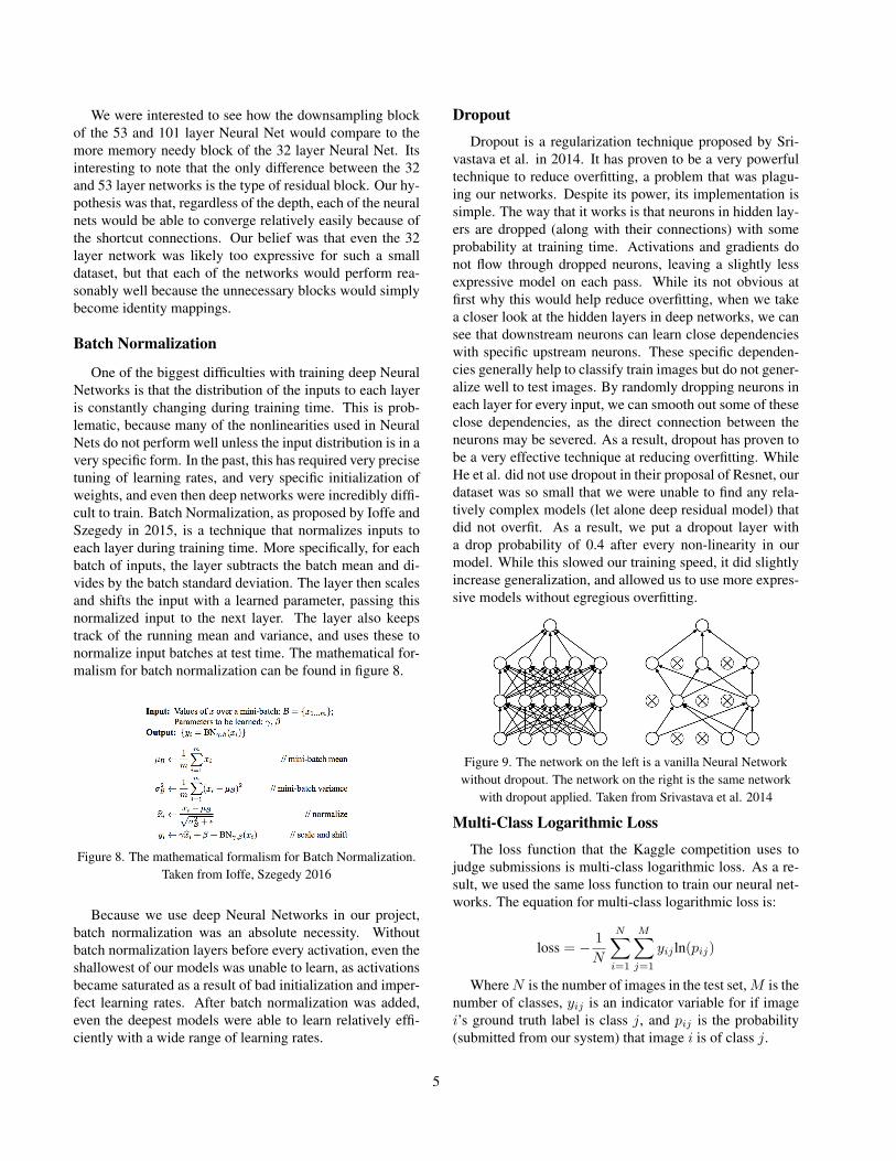
One of the biggest difficulties with training deep NeuralNetworks is that the distribution of the inputs to each layeris constantly changing during training time. This is prob-lematic, because many of the nonlinearities used in NeuralNets do not perform well unless the input distribution is in avery specific form. In the past, this has required very precisetuning of learning rates, and very specific initialization ofweights, and even then deep networks were incredibly diffi-cult to train. Batch Normalization, as proposed by Ioffe andSzegedy in 2015, is a technique that normalizes inputs toeach layer during training time. More specifically, for eachbatch of inputs, the layer subtracts the batch mean and di-vides by the batch standard deviation. The layer then scalesand shifts the input with a learned parameter, passing thisnormalized input to the next layer. The layer also keepstrack of the running mean and variance, and uses these tonormalize input batches at test time. The mathematical for-malism for batch normalization can be found in figure 8.
Figure 8. The mathematical formalism for Batch Normalization.Taken from Ioffe, Szegedy 2016
Because we use deep Neural Networks in our project,batch normalization was an absolute necessity. Withoutbatch normalization layers before every activation, even theshallowest of our models was unable to learn, as activationsbecame saturated as a result of bad initialization and imper-fect learning rates. After batch normalization was added,even the deepest models were able to learn relatively effi-ciently with a wide range of learning rates.
Dropout
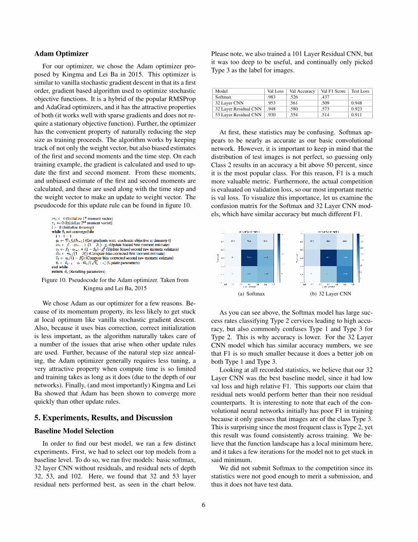
Dropout is a regularization technique proposed by Sri-vastava et al. in 2014. It has proven to be a very powerfultechnique to reduce overfitting, a problem that was plagu-ing our networks. Despite its power, its implementation issimple. The way that it works is that neurons in hidden lay-ers are dropped (along with their connections) with someprobability at training time. Activations and gradients donot flow through dropped neurons, leaving a slightly lessexpressive model on each pass. While its not obvious atfirst why this would help reduce overfitting, when we takea closer look at the hidden layers in deep networks, we cansee that downstream neurons can learn close dependencieswith specific upstream neurons. These specific dependen-cies generally help to classify train images but do not gener-alize well to test images. By randomly dropping neurons ineach layer for every input, we can smooth out some of theseclose dependencies, as the direct connection between theneurons may be severed. As a result, dropout has proven tobe a very effective technique at reducing overfitting. WhileHe et al. did not use dropout in their proposal of Resnet, ourdataset was so small that we were unable to find any rela-tively complex models (let alone deep residual model) thatdid not overfit. As a result, we put a dropout layer witha drop probability of 0.4 after every non-linearity in ourmodel. While this slowed our training speed, it did slightlyincrease generalization, and allowed us to use more expres-sive models without egregious overfitting.
Figure 9. The network on the left is a vanilla Neural Networkwithout dropout. The network on the right is the same network
with dropout applied. Taken from Srivastava et al. 2014
Multi-Class Logarithmic Loss
The loss function that the Kaggle competition uses tojudge submissions is multi-class logarithmic loss. As a re-sult, we used the same loss function to train our neural net-works. The equation for multi-class logarithmic loss is:
loss = − 1
N
N∑i=1
M∑j=1
yij ln(pij)
Where N is the number of images in the test set, M is thenumber of classes, yij is an indicator variable for if imagei’s ground truth label is class j, and pij is the probability(submitted from our system) that image i is of class j.
5
Adam Optimizer
For our optimizer, we chose the Adam optimizer pro-posed by Kingma and Lei Ba in 2015. This optimizer issimilar to vanilla stochastic gradient descent in that its a firstorder, gradient based algorithm used to optimize stochasticobjective functions. It is a hybrid of the popular RMSPropand AdaGrad optimizers, and it has the attractive propertiesof both (it works well with sparse gradients and does not re-quire a stationary objective function). Further, the optimizerhas the convenient property of naturally reducing the stepsize as training proceeds. The algorithm works by keepingtrack of not only the weight vector, but also biased estimatesof the first and second moments and the time step. On eachtraining example, the gradient is calculated and used to up-date the first and second moment. From these moments,and unbiased estimate of the first and second moments arecalculated, and these are used along with the time step andthe weight vector to make an update to weight vector. Thepseudocode for this update rule can be found in figure 10.
Figure 10. Pseudocode for the Adam optimizer. Taken fromKingma and Lei Ba, 2015
We chose Adam as our optimizer for a few reasons. Be-cause of its momentum property, its less likely to get stuckat local optimum like vanilla stochastic gradient descent.Also, because it uses bias correction, correct initializationis less important, as the algorithm naturally takes care ofa number of the issues that arise when other update rulesare used. Further, because of the natural step size anneal-ing, the Adam optimizer generally requires less tuning, avery attractive property when compute time is so limitedand training takes as long as it does (due to the depth of ournetworks). Finally, (and most importantly) Kingma and LeiBa showed that Adam has been shown to converge morequickly than other update rules.
5. Experiments, Results, and DiscussionBaseline Model Selection
In order to find our best model, we ran a few distinctexperiments. First, we had to select our top models from abaseline level. To do so, we ran five models: basic softmax,32 layer CNN without residuals, and residual nets of depth32, 53, and 102. Here, we found that 32 and 53 layerresidual nets performed best, as seen in the chart below.
Please note, we also trained a 101 Layer Residual CNN, butit was too deep to be useful, and continually only pickedType 3 as the label for images.
Model Val Loss Val Accuracy Val F1 Score Test LossSoftmax .983 .526 .437 -32 Layer CNN .953 .561 .509 0.94832 Layer Residual CNN .948 .580 .573 0.92353 Layer Residual CNN .930 .554 .514 0.911
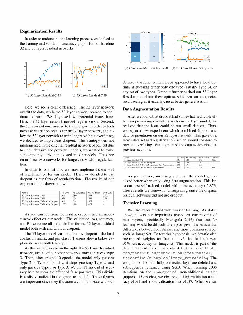
At first, these statistics may be confusing. Softmax ap-pears to be nearly as accurate as our basic convolutionalnetwork. However, it is important to keep in mind that thedistribution of test images is not perfect, so guessing onlyClass 2 results in an accuracy a bit above 50 percent, sinceit is the most popular class. For this reason, F1 is a muchmore valuable metric. Furthermore, the actual competitionis evaluated on validation loss, so our most important metricis val loss. To visualize this importance, let us examine theconfusion matrix for the Softmax and 32 Layer CNN mod-els, which have similar accuracy but much different F1.
(a) Softmax (b) 32 Layer CNN
As you can see above, the Softmax model has large suc-cess rates classifying Type 2 cervices leading to high accu-racy, but also commonly confuses Type 1 and Type 3 forType 2. This is why accuracy is lower. For the 32 LayerCNN model which has similar accuracy numbers, we seethat F1 is so much smaller because it does a better job onboth Type 1 and Type 3.
Looking at all recorded statistics, we believe that our 32Layer CNN was the best baseline model, since it had lowval loss and high relative F1. This supports our claim thatresidual nets would perform better than their non residualcounterparts. It is interesting to note that each of the con-volutional neural networks initially has poor F1 in trainingbecause it only guesses that images are of the class Type 3.This is surprising since the most frequent class is Type 2, yetthis result was found consistently across training. We be-lieve that the function landscape has a local minimum here,and it takes a few iterations for the model not to get stuck insaid minimum.
We did not submit Softmax to the competition since itsstatistics were not good enough to merit a submission, andthus it does not have test data.
6
Regularization Results
In order to understand the learning process, we looked atthe training and validation accuracy graphs for our baseline32 and 53 layer residual networks:
(c) 32 Layer Residual CNN (d) 53 Layer Residual CNN
Here, we see a clear difference. The 32 layer networkoverfit the data, while the 53 layer network seemed to con-tinue to learn. We diagnosed two potential issues here.First, the 32 layer network needed regularization. Second,the 53 layer network needed to train longer. In order to bothincrease validation results for the 32 layer network, and al-low the 53 layer network to train longer without overfitting,we decided to implement dropout. This strategy was notimplemented in the original residual network paper, but dueto small datasize and powerful models, we wanted to makesure some regularization existed in our models. Thus, wereran these two networks for longer, now with regulariza-tion.
In order to combat this, we must implement some sortof regularization for our model. Here, we decided to usedropout as our form of regularization. The results of ourexperiment are shown below:
Model Val Loss Val Accuracy Val F1 Score Test Loss32 Layer Residual CNN .948 .580 .573 0.92353 Layer Residual CNN .930 .554 .514 0.91132 Layer Residual CNN with Dropout .948 .564 .567 -53 Layer Residual CNN with Dropout 1.072 .499 .467 -
As you can see from the results, dropout had an incon-clusive effect on our model. The validation loss, accuracy,and F1 score are all quite similar for the 32 layer residualmodel both with and without dropout.
The 53 layer model was hindered by dropout - the finalconfusion matrix and per class F1 scores shown below ex-plain its issues with training:
As the reader can see on the right, the 53 Layer Residualnetwork, like all of our other networks, only can guess Type3. Then, after around 10 epochs, the model only guessesType 2 or Type 3. Finally, it stops guessing Type 2, andonly guesses Type 1 or Type 3. We plot F1 instead of accu-racy here to show the effect of false positives. This divideis easily visualized in the graph to the left. These figuresare important since they illustrate a common issue with our
(e) Confusion Matrix at Epoch 70 (f) Per Class F1 over 70 Epochs
dataset - the function landscape appeared to have local op-tima at guessing either only one type (usually Type 3), orany set of two types. Dropout further pushed our 53 LayerResidual model into these optima, which was an unexpectedresult seeing as it usually causes better generalization.
Data Augmentation Results
After we found that dropout had somewhat negligible ef-fect on preventing overfitting with our 32 layer model, werealized that the issue could be our small dataset. Thus,we began a new experiment which combined dropout anddata augmentation on our 32 layer network. This gave us alarger data set and regularization, which should combine toprevent overfitting. We augmented the data as described inprevious sections.
Model Val Loss Val Accuracy Val F1 Score Test Loss32 Layer Residual CNN .948 .580 .573 0.92332 Layer Residual CNN with Dropout .948 .564 .567 -32 Layer Residual CNN with Dropout and Data Augmentation .936 .576 .551 -32 Layer Residual CNN with Data Augmentation .879 .588 .578 .873
As you can see, surprisingly enough the model gener-alized better when only using data augmentation. This ledto our best self trained model with a test accuracy of .873.These results are somewhat unsurprising, since the originalresidual networks did not use dropout.
Transfer Learning
We also experimented with transfer learning. As statedabove, it was our hypothesis (based on our reading ofpast papers, specifically Menegola 2016) that transferlearning would be difficult to employ given the substantialdifferences between our dataset and more common sourcessuch as ImageNet. To test this hypothesis, we downloadedpre-trained weights for Inception v3 that had achieved95% test accuracy on Imagenet. This model is part of thedefault Tensorflow source code at https://github.com/tensorflow/tensorflow/tree/master/tensorflow/examples/image_retraining. Theweights for the final fully-connected layer are deleted andsubsequently retrained using SGD. When running 2000iterations on the un-augmented, non-additional dataset(approx. 15 epochs), we observed a high validation accu-racy of .61 and a low validation loss of .87. When we ran
7
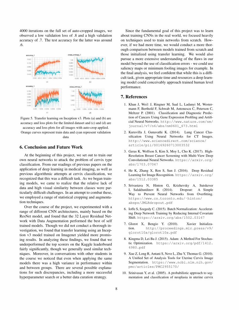
4000 iterations on the full set of auto-cropped images, weobserved a low validation loss of .8 and a high validationaccuracy of .7. The test accuracy for the latter was around.6.
Figure 5. Transfer learning on Inception v3. Plots (a) and (b) areaccuracy and loss plots for the limited dataset and (c) and (d) are
accuracy and loss plots for all images with auto-crop applied.Orange curves represent train data and cyan represent validation
data
6. Conclusion and Future Work
At the beginning of this project, we set out to train ourown neural networks to attack the problem of cervix typeclassification. From our readings of previous papers on theapplication of deep learning in medical imaging, as well asprevious algorithmic attempts at cervix classification, werecognized that this was a difficult task. As we began train-ing models, we came to realize that the relative lack ofdata and high visual similarity between classes were par-ticularly difficult challenges. In an attempt to combat these,we employed a range of statistical cropping and augmenta-tion techniques.
Over the course of the project, we experimented with arange of different CNN architectures, mainly based on theResNet model, and found that the 32 Layer Residual Net-work with Data Augmentation performed the best of selftrained models. Though we did not conduct a thorough in-vestigation, we found that transfer learning using an Incep-tion v3 model trained on Imagenet yielded more promis-ing results. In analyzing these findings, we found that weunderperformed the top scorers on the Kaggle leaderboardfairly significantly, though we generally used similar tech-niques. Moreover, in conversations with other students inthe course we noticed that even when applying the samemodels there was a high variance in performance withinand between groups. There are several possible explana-tions for such discrepancies, including a more successfulhyperparameter search or a better data curation strategy.
Since the fundamental goal of this project was to learnabout training CNNs in the real world, we focused heavilyon techniques used to train networks from scratch. How-ever, if we had more time, we would conduct a more thor-ough comparison between models trained from scratch andthose initialized using transfer learning. We would alsopursue a more extensive understanding of the flaws in ourmodel beyond the use of classification errors - we could usesaliency maps or minimum fooling images for example. Inthe final analysis, we feel confident that while this is a diffi-cult task, given appropriate time and resources a deep learn-ing model could conceivably approach trained human levelperformance.
7. References1. Khan J, Wei1 J, Ringner M, Saal L, Ladanyi M, Wester-
mann F, Berthold F, Schwab M, Antonescu C, Peterson C,Meltzer P. (2001). Classification and Diagnostic Predic-tion of Cancers Using Gene Expression Profiling and Artifi-cial Neural Networks. http://www.nature.com/nm/journal/v7/n6/abs/nm0601_673.html
2. Kuruvilla J, Gunavathi K. (2014). Lung Cancer Clas-sification Using Neural Networks for CT Images.http://www.sciencedirect.com/science/article/pii/S0169260713003532
3. Geras K, Wolfson S, Kim S, Moy L, Cho K. (2017). High-Resolution Breast Cancer Screening with Multi-View DeepConvolutional Neural Networks. https://arxiv.org/abs/1703.07047
4. He K, Zhang X, Ren S, Sun J. (2016). Deep ResidualLearning for Image Recognition. https://arxiv.org/abs/1512.03385
5. Srivastava N, Hinton G, Krizhevsky A, SutskeverI, Salakhutdinov R. (2014). Dropout: A SimpleWay to Prevent Neural Networks from Overfitting.https://www.cs.toronto.edu/˜hinton/absps/JMLRdropout.pdf
6. Ioffe S, Szegedy C. (2015). Batch Normalization: Accelerat-ing Deep Network Training by Reducing Internal CovariateShift. https://arxiv.org/abs/1502.03167
7. Glorot X, Bengio Y. (2010). Xavier Initializa-tion. http://proceedings.mlr.press/v9/glorot10a/glorot10a.pdf
8. Kingma D, Lei Ba J. (2015). Adam: A Method For Stochas-tic Optimization. https://arxiv.org/pdf/1412.6980.pdf
9. Xue Z, Long R, Antani S, Neve L, Zhu Y, Thomas G. (2010).A Unified Set of Analysis Tools for Uterine Cervix ImageSegmentation. https://www.ncbi.nlm.nih.gov/pmc/articles/PMC2955170/
10. Srinivasan Y, et al. (2005). A probabilistic approach to seg-mentation and classification of neoplasia in uterine cervix
8
images using color and geometric features. International So-ciety for Optics and Photonics. https://lhncbc.nlm.nih.gov/files/archive/pub2005015.pdf
11. Gordon S, Zimmerman G, Greenspan H. (2004). Im-age segmentation of uterine cervix images for in-dexing in PACS. http://ieeexplore.ieee.org/abstract/document/1311731/
12. Litjens, G., Kooi, T., Ehteshami, B., et al. A Survey onDeep Learning in Medical Image Analysis. 2017. https://arxiv.org/abs/1702.05747
13. Liu, Y., Gadepalli, K., Norouzi, M., Dahl, G. E., Kohlberger,T., Boyko, A., Venugopalan, S., Timofeev, A., Nelson, P. Q.,Corrado, G. S., Hipp, J. D., Peng, L., Stumpe, M. C., 2017.Detecting cancer metastases on gigapixel pathology images.arXiv:1703.02442
14. Antony, J., McGuinness, K., Connor, N. E. O., Moran,K., 2016. Quantifying radiographic knee osteoarthri-tis severity using deep convolutional neural networks.arXiv:1609.02469.
15. Menegola, A., Fornaciali, M., Pires, R., Avila, S., Valle, E.,2016. Towards automated melanoma screening: Exploringtransfer learning schemes. arXiv:1609.01228.
16. Esteva, A., Kuprel, B., Novoa, R. A., Ko, J., Swetter, S. M.,Blau, H. M., Thrun, S., 2017. Dermatologist-level classifica-tion of skin cancer with deep neural networks. Nature 542,115118.
17. Ronneberger, O., Fischer, P., Brox, T., 2015. U-net: Con-volutional networks for biomedical image segmentation. In:Med Image Comput Comput Assist Interv. Vol. 9351 of LectNotes Comput Sci. pp. 234241
18. Armato, S. G., McLennan, G., Bidaut, L., McNitt-Gray, M.F., Meyer, C. R., Reeves, A. P., Zhao, et al. 2011. The lungimage database consortium (LIDC) and image database re-source initiative (IDRI): a completed reference database oflung nodules on CT scans. Med Phys 38, 915931.
19. Pereira, S., Pinto, A., Alves, V., Silva, C. A., 2016. Braintumor segmentation using convolutional neural networks inMRI images. IEEE Trans Med Imaging.
20. Sirinukunwattana, K., Raza, S. E. A., Tsang, Y.-W., Snead,D. R., Cree, I. A., Rajpoot, N. M., 2016. Locality sensi-tive deep learning for detection and classification of nucleiin routine colon cancer histology images. IEEE Trans MedImaging 35 (5), 11961206.
21. Greenspan H, Gordon S, Zimmerman G, et al. 2009.Automatic Detection of Anatomical Landmarks in UterineCervix Images. IEEE TRANSACTIONS ON MEDI-CAL IMAGING. https://www.researchgate.net/publication/24041301_Automatic_Detection_of_Anatomical_Landmarks_in_Uterine_Cervix_Images
22. User:Chattob. 2017. Cervix segmentation (GMM).https://www.kaggle.com/chattob/cervix-segmentation-gmm/notebook
23. User:aleju. 2017. imgaug: Image augmentation for machinelearning experiments. https://github.com/aleju/imgaug
9