INTEGRATION TO GENERATE MOTIVATION TO LEARN

INTEGRATION TO FOSTER CREATIVITY

WHO’S HU IN EDTEK ’04

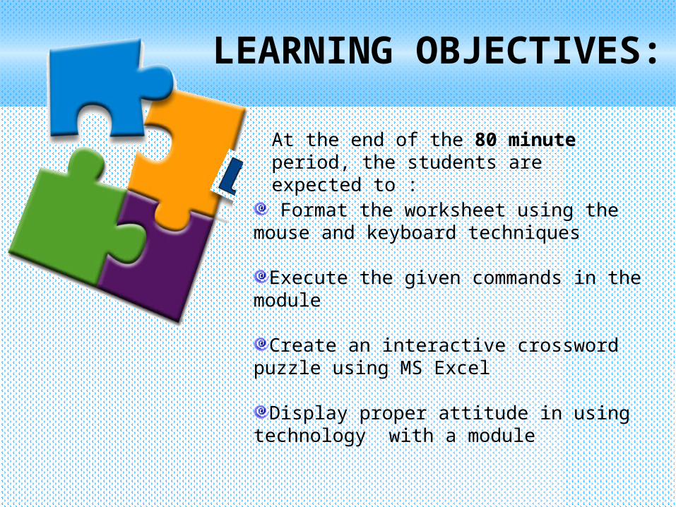
LEARNING OBJECTIVES:

At the end of the 80 minute period, the students are expected to :

Format the worksheet using the mouse and keyboard techniques

Execute the given commands in the module

Create an interactive crossword puzzle using MS Excel

Display proper attitude in using technology with a module

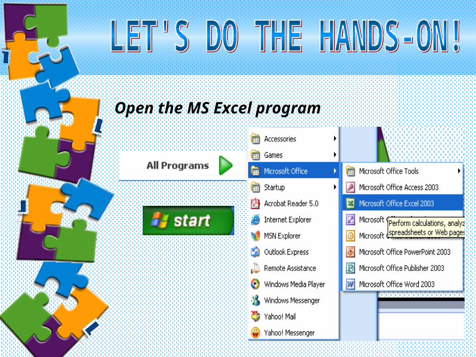
Open the MS Excel program

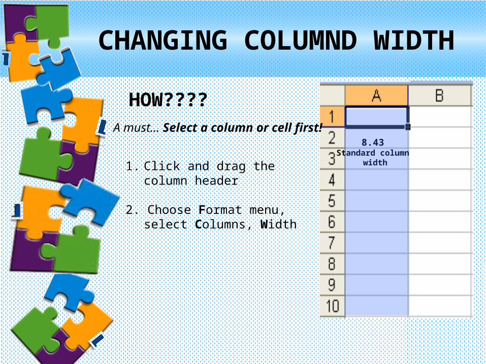
CHANGING COLUMND WIDTH

HOW????A must… Select a column or cell first!

1. Click and drag the column header

2. Choose Format menu, select Columns, Width

8.43Standard column

width

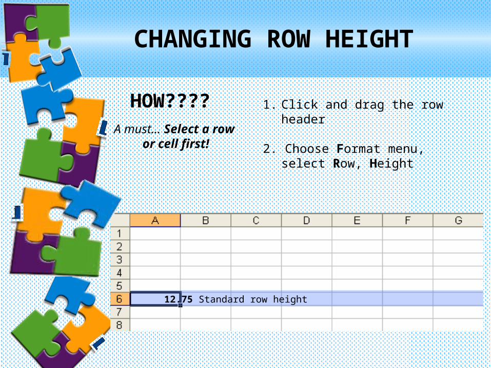
CHANGING ROW HEIGHT

HOW????A must… Select a row

or cell first!

1. Click and drag the row header

2. Choose Format menu, select Row, Height

12.75 Standard row height

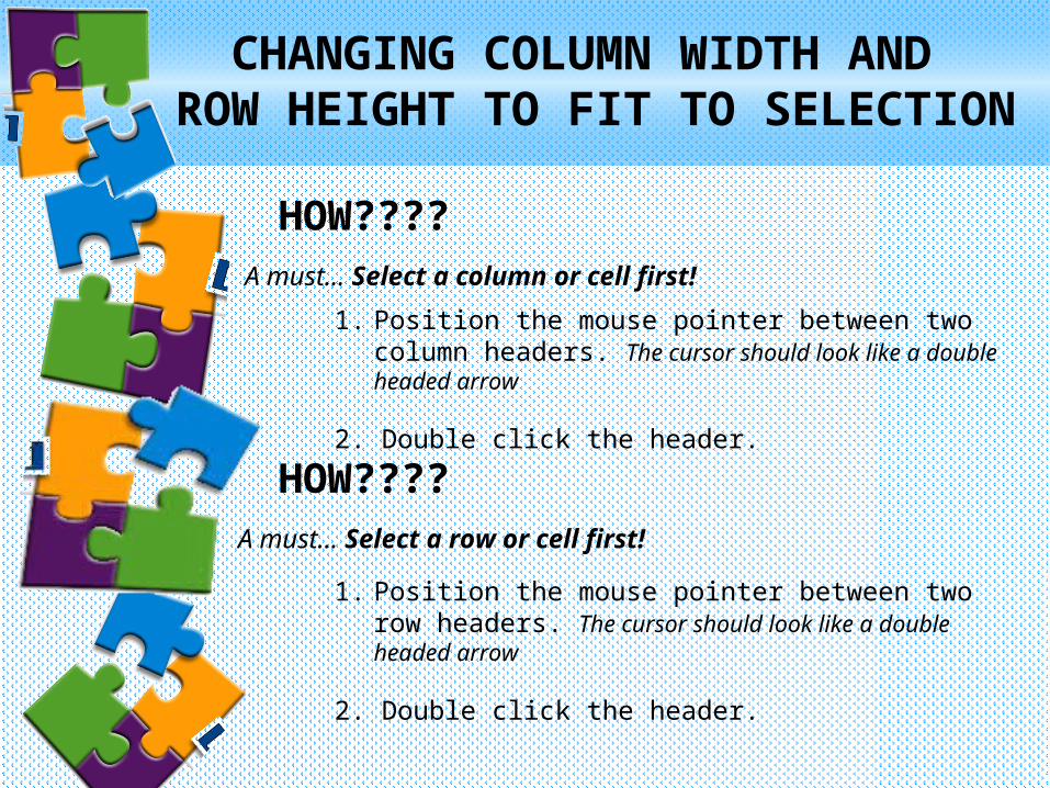
CHANGING COLUMN WIDTH AND ROW HEIGHT TO FIT TO SELECTION

HOW????A must… Select a column or cell first!

HOW????A must… Select a row or cell first!

1. Position the mouse pointer between two row headers. The cursor should look like a double headed arrow

2. Double click the header.

1. Position the mouse pointer between two column headers. The cursor should look like a double headed arrow

2. Double click the header.

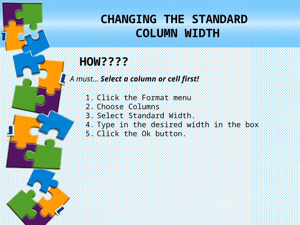
CHANGING THE STANDARD COLUMN WIDTH

HOW????A must… Select a column or cell first!

1. Click the Format menu2. Choose Columns3. Select Standard Width. 4. Type in the desired width in the box5. Click the Ok button.

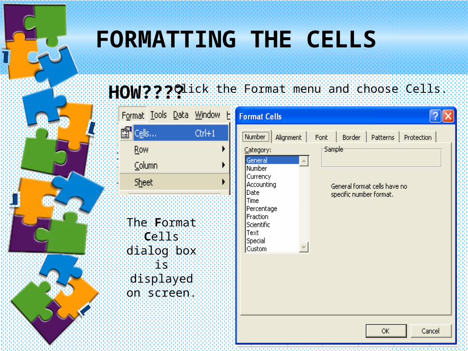
FORMATTING THE CELLS

HOW???? Click the Format menu and choose Cells.

The Format Cells dialog

box is displayed on

screen.

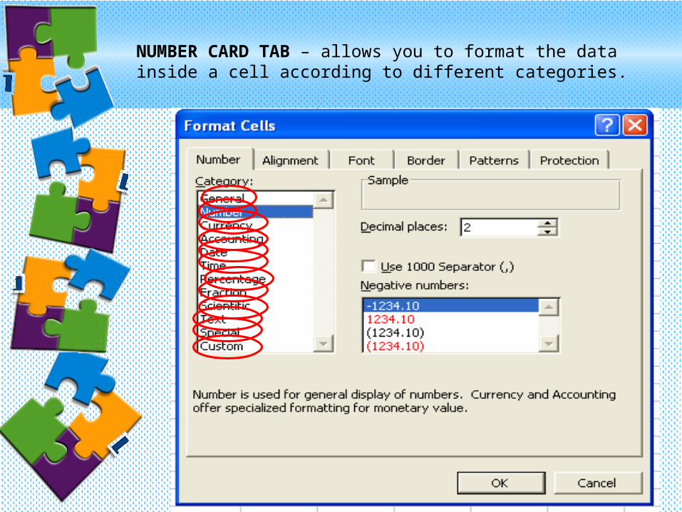
NUMBER CARD TAB – allows you to format the data inside a cell according to different categories.

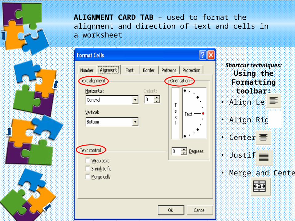
ALIGNMENT CARD TAB – used to format the alignment and direction of text and cells in a worksheet

Shortcut techniques:

Using the Formatting

toolbar:

• Align Left

• Align Right

• Center

• Justify

• Merge and Center

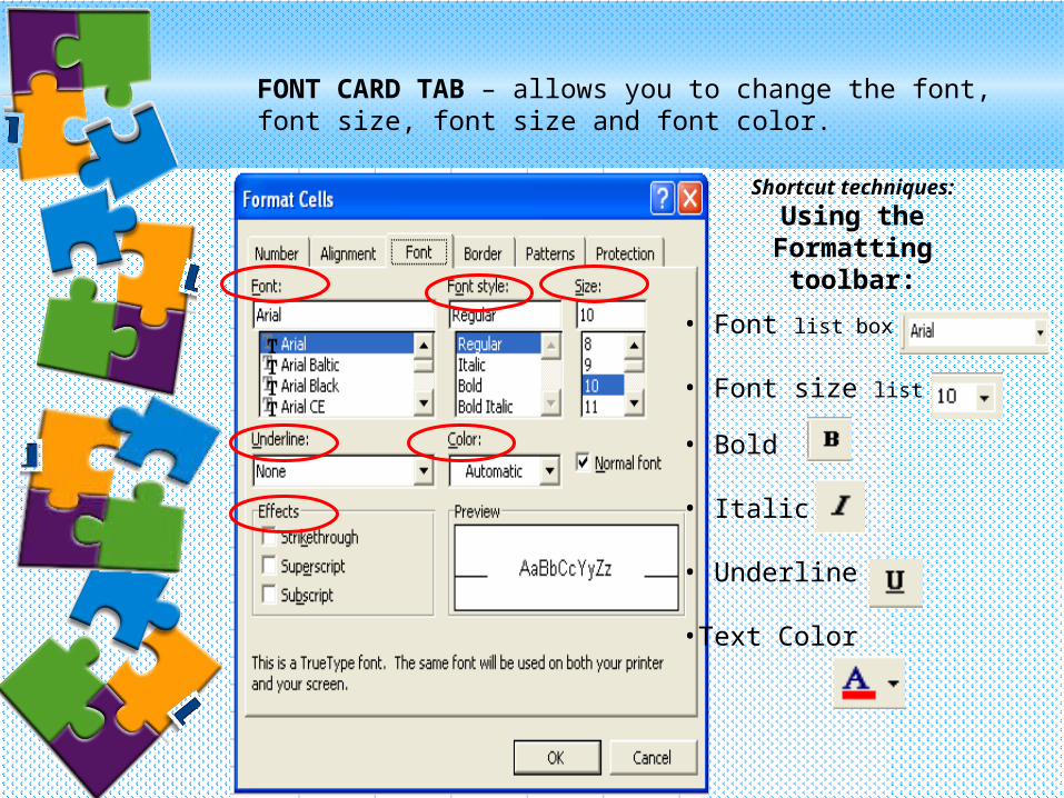
FONT CARD TAB – allows you to change the font, font size, font size and font color.

Shortcut techniques:

Using the Formatting

toolbar:

• Font list box

• Font size list box

• Bold

• Italic

• Underline

•Text Color

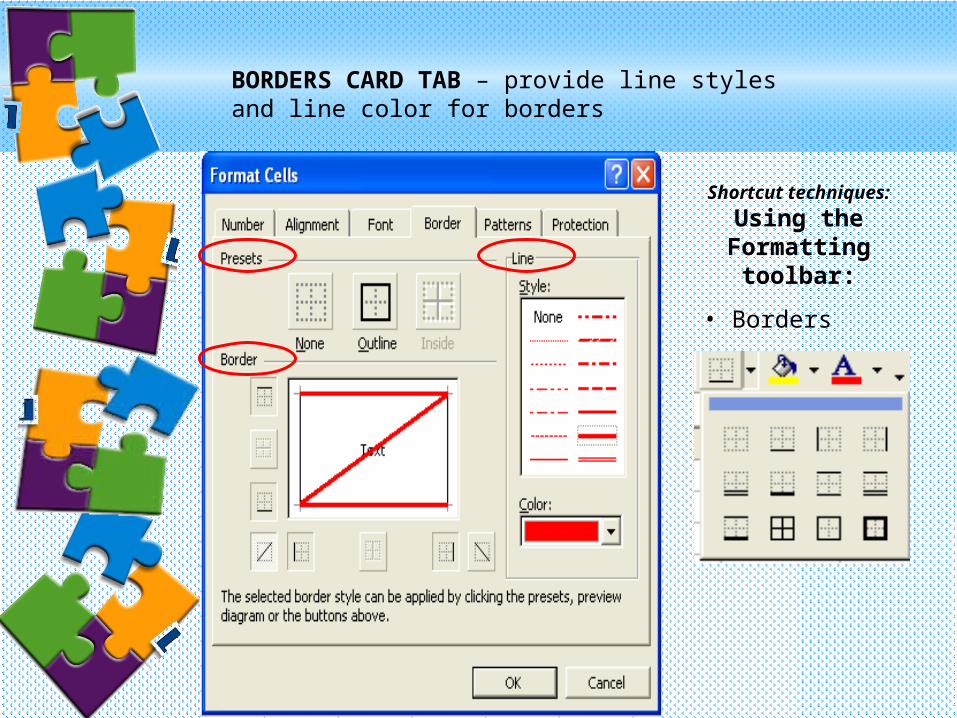
BORDERS CARD TAB – provide line styles and line color for borders

Shortcut techniques:

Using the Formatting

toolbar:

• Borders

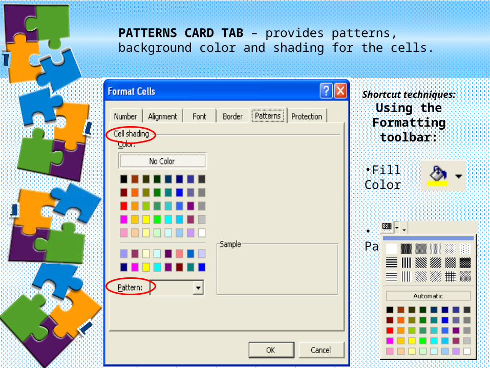
PATTERNS CARD TAB – provides patterns, background color and shading for the cells.

Shortcut techniques:

Using the Formatting

toolbar:

•Fill Color

• Fill Patterns

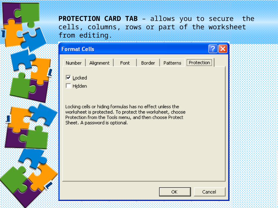
PROTECTION CARD TAB – allows you to secure the cells, columns, rows or part of the worksheet from editing.

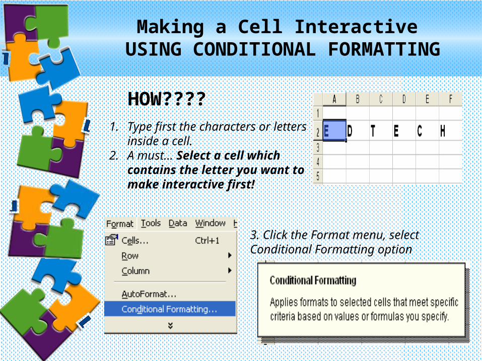
Making a Cell Interactive USING CONDITIONAL FORMATTING

HOW????1. Type first the characters or letters

inside a cell.2. A must… Select a cell which

contains the letter you want to make interactive first!

3. Click the Format menu, select Conditional Formatting option

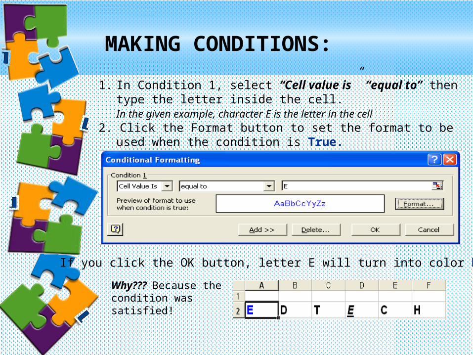
1. In Condition 1, select “Cell value is” “equal to” then type the letter inside the cell. In the given example, character E is the letter in the cell

2. Click the Format button to set the format to be used when the condition is True.

MAKING CONDITIONS:

If you click the OK button, letter E will turn into color blue

Why??? Because the condition was satisfied!

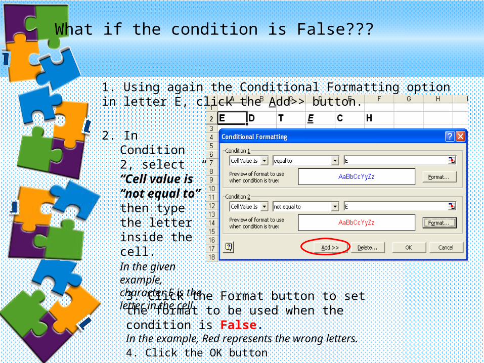
What if the condition is False???

1. Using again the Conditional Formatting option in letter E, click the Add>> button.

2. In Condition 2, select “Cell value is” “not equal to” then type the letter inside the cell. In the given example, character E is the letter in the cell

3. Click the Format button to set the format to be used when the condition is False.In the example, Red represents the wrong letters.4. Click the OK button

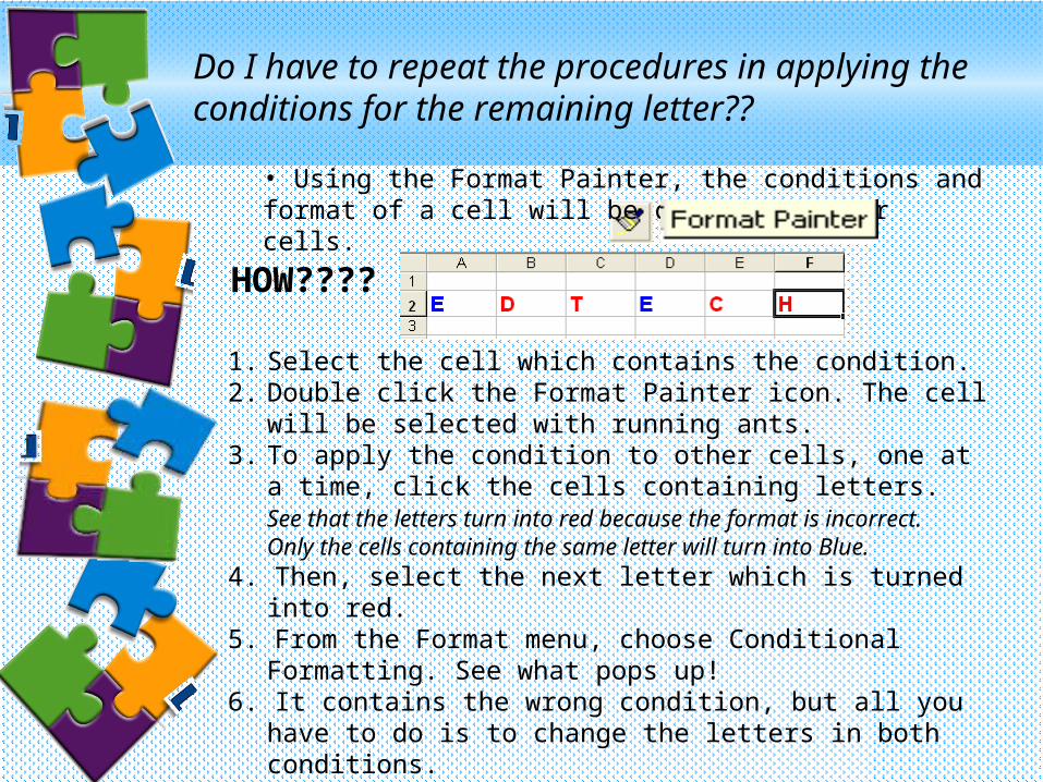
Do I have to repeat the procedures in applying the conditions for the remaining letter??

• Using the Format Painter, the conditions and format of a cell will be copied to other cells.

HOW????

1. Select the cell which contains the condition.2. Double click the Format Painter icon. The cell will be selected

with running ants.3. To apply the condition to other cells, one at a time, click the

cells containing letters. See that the letters turn into red because the format is incorrect. Only the cells containing the same letter will turn into Blue.

4. Then, select the next letter which is turned into red. 5. From the Format menu, choose Conditional Formatting. See

what pops up!6. It contains the wrong condition, but all you have to do is to

change the letters in both conditions.7. Repeat the process until all letters turn into blue.

EASY RIGHT?????

YOU ARE NOW READY TO CREATE YOUR OWN INTERACTIVE CROSSWORD PUZZLE!!!

Asking about the questions? Huh?!!

Very simple….

1. Select e cell containing the letter.2. Click the right mouse button.3. Choose Add comments4. Then type the questions…

Here are some questions…questions…questions… and questions…????

But before that?

What is the important rule before formatting a cell?

What are the techniques in formatting the worksheet?

What menu can be used to make changes with your cells?

2.   How can we make a cell interactive? What are the commands to be used?

Create a puzzle of your own!!!

• Think of your topic (it can be about yourself, your favorite subject or something that you are interested with)• List at least five to ten word with their corresponding questions.• Open MS Excel program and format the worksheet.• Plot the words in the worksheet and apply formatting.• Create and design your own interactive crossword puzzle. Put a title for the puzzle• Save it using Puzzle_your surname as the filename inside your folder.

Don’t forget to let your classmates try your puzzle…

Don’t forget to let your classmates try your puzzle…

Let me show you another puzzle…

Philippine Normal UniversityMaster in Educational Technology

Presented by: Ms. Wilma B. Rollon

EdTech 501