Chapter 6

Integration

In this chapter we define the integral. Intuitively, it should be the area undera curve. Not surprisingly, after many examples, counter examples, exceptions,generalizations, the concept of the integral may seem strange. And not surprisingly,there is more than one way to define the integral. We start with the Darbouxintegral and later show it is equivalent to the Riemann integral.

6.1. Darboux Integral

Throughout this chapter we assume [a, b] be a closed, bounded interval, and thatthe functions f : [a, b] → R under consideration are bounded.

Definition 6.1. Let [a, b] be a closed, bounded interval.

(i) A Partition of [a, b] is a set of points P = {x0, x1, x2, . . . , xn−1, xn} witha = x0 < x1 < · · · < xn = b.

(ii) The norm of a partition is kPk = max1≤i≤n

|xi − xi−1|.

(iii) A Refinement of P is a partition Q of [a, b] such that P ⊆ Q. We say Q isfiner than P .

Note that kQk ≤ kPk. In addition, if P and Q are partition of [a, b], P ∪ Q isfiner than both P and Q.

Definition 6.2. Let f : [a, b] → R be bounded. Set

Mj(f) = supxj−1≤x≤xj

f(x) mj(f) = infxj−1≤x≤xj

f(x).

(a) The upper-Darboux Sum of f over P is

U(P, f) =

nX

j=1

Mj(f)(xj − xj−1).

65

66 6. Integration

(b) The lower-Darboux Sum of f over P is

L(P, f) =

nX

j=1

mj(f)(xj − xj−1).

The following lemma provides a relationship between the upper/lower Darbouxsums and partitions.

Lemma 6.3. Let P be any partition of [a, b] and Q be any refinement of P . Then

L(P, f) ≤ L(Q, f) ≤ U(Q, f) ≤ U(P, f).

Proof. Let P = {x0, x1, . . . , xn}. By assumption P ⊆ Q. Let us suppose onepoint, z, has been added to P . Specifically, suppose xj−1 < z < xj for some j. Callthe new partition P ′. Let

Mj(f) = sup{f(x) : x ∈ [xj−1, xj ]}, mj(f) = inf{f(x) : x ∈ [xj−1, xj ]},β1(f) = inf{f(x) : x ∈ [xj−1, z]}, β2(f) = inf{f(x) : x ∈ [z, xj]}.

Note mj ≤ β1 and mj ≤ β2 since mj is the infimum over a larger set. Moreover,we may write xj − xj−1 = (xj − z) + (z − xj−1). Thus

L(P, f) =nX

i=1

mi(f)(xi − xi−1)

=

j−1X

i=1

mi(f)(xi − xi−1) +mj(f)(xj − xj−1) +nX

i=j+1

mi(f)(xi − xi−1)

≤j−1X

i=1

mi(f)(xi − xi−1) + β1(z − xj−1) + β2(xj − z)

+

nX

i=j+1

mi(f)(xi − xi−1)

= L(P ′, f)

A similar argument shows U(P, f) ≥ U(P ′, f). If Q contains points not in P , werepeat the argument (there can only be a finite number of additional points) toobtain L(P, f) ≤ L(Q, f) and U(Q, f) ≤ U(P, f). The definition of the upper andlower sums implies L(Q, f) ≤ U(Q, f), and the inequality follows. �

Corollary 6.4. We have L(P, f) ≤ U(Q, f) for any partitions P and Q of [a, b].

Proof. Since P ∪Q is a refinement of both P and Q,

L(P, f) ≤ L(P ∪Q, f) ≤ U(P ∪Q, f) ≤ U(Q, f).

�We are ready to define the integral.

Definition 6.5. The function f : [a, b] → R is said to be Darboux Integrable on[a, b] if and only if f is bounded and, for all ǫ > 0, there exists a partition, P , of[a, b] such that U(P, f)−L(P, f) < ǫ. In this case we say f ∈ R[a, b] (the R standsfor Riemann).

6.1. Darboux Integral 67

Note the definition of the existence of the integral does not say what the integralis.

Definition 6.6. Let f : [a, b] → R be bounded. Set

(i)

Z b

a

f(x) dx = inf{U(P, f) | P a partition of [a, b]}

(ii)

Z b

a

f(x) dx = sup{L(P, f) | P a partition of [a, b]}

If

Z b

a

f(x) dx =

Z b

a

f(x) dx, we say the integral of f is

Z b

a

f(x) dx.

You might wonder why the sup and inf exist in the definition.

Lemma 6.7. If f : [a, b] → R is bounded, then both

Z b

a

f(x) dx and

Z b

a

f(x) dx

exist. Moreover,Z b

a

f(x) dx ≤Z b

a

f(x) dx.

Proof. Recall that L(P, f) ≤ U(Q, f) for any partitions P , Q of [a, b]. Thus thenumbers L(P, f) are bounded above and by the completeness axiom sup

PL(P, f)

exists. Similarly, U(Q, f) is bounded below by any L(P, f), and so infP

U(P, f)

exist.

Taking the supremum of the left side of the inequality L(P, f) ≤ U(Q, f), wefind

Z b

a

f(x) dx ≤ U(Q, f).

Taking the infimum of the right side provides the inequality in the lemma. �

You might hope too that f ∈ R[a, b] impliesR b

a f(x) dx exists.

Theorem 6.8. Suppose f ∈ R[a, b]. Then

Z b

a

f(x) dx =

Z b

a

f(x) dx.

Proof. Since f ∈ R[a, b], for all ǫ > 0, there exists a partition of [a, b] such thatU(P, f)− L(P, f) < ǫ. Thus

L(P, f) ≤Z b

a

f(x) dx ≤Z b

a

f(x) dx ≤ U(P, f).

That is,

0 ≤Z b

a

f(x) dx−Z b

a

f(x) dx ≤ U(P, f)− L(P, f) < ǫ,

and the result follows. �

68 6. Integration

Example 6.9. Prove the function

f(x) =

�

1 0 ≤ x < 1,2 x = 1.

is in R[0, 1] and find the integral.

Proof. Let ǫ > 0. Set P = {0, 1− ǫ2 , 1}. Then

M1(f) = 1 = m1(f),

and M2(f) = 2,m2(f) = 1 (a sketch of the function and the partition might beuseful). Thus

U(P, f) = 1�

1− ǫ

2− 0

�

+ 2�

1− (1 − ǫ

2)�

= 1 +ǫ

2

L(P, f) = 1�

1− ǫ

2− 0

�

+ 1�

1− (1− ǫ

2)�

= 1,

and hence U(P, f)− L(P, f) = ǫ/2 < ǫ and f ∈ R[0, 1].

To find the integral note

L(P, f) ≤Z 1

0

f(x) dx ≤ U(P, f)

or

1 ≤Z 1

0

f(x) dx ≤ 1 +ǫ

2

which implies

Z 1

0

f(x) dx = 1. �

Example 6.10. Show that Dirichlet’s function

f(x) =

�

1 x ∈ Q,0 x ∈ Qc.

is not in R[0, 1].

Proof. To show a function is not integrable we must show the existence of a ǫ0 > 0such that for all partitions of [a, b], U(P, f) − L(P, f) ≥ ǫ0. Let ǫ0 = 1/2. For anypartition of [0, 1] we have Mj(f) = 1 and mj(f) = 0. Thus

U(P, f)− L(P, f) = U(P, f)− 0 =nX

j=1

1(xj − xj−1) = 1 ≥ ǫ0

and f is not integrable. �

Integrable functions can be complicated as the next example shows.

Example 6.11. Consider the function on [0, 1]

f(x) =

1 x = 1n

0 x 6= 1n .

Prove f ∈ R[0, 1]; i.e. f is Darboux integrable and find the integral.

6.1. Darboux Integral 69

Proof. Let ǫ > 0. By the Archimedean Property an n0 ∈ N exists so that 2/ǫ < n0.That is 1/n0 < ǫ/2. By the Well-Ordering Property, a minimum such n0 (againcalled n0) exists. That is,

(6.1)1

n0<

ǫ

2≤ 1

n0 − 1.

We assume, without loss of generality, that n0 > 2.

Behold: Set P to be the partition

P =

�

0,1

n0+

ǫ2

16,

1

n0 − 1− ǫ2

16,

1

n0 − 1+

ǫ2

16,

1

n0 − 2− ǫ2

16,

1

n0 − 2+

ǫ2

16,

. . . , 1− ǫ2

16, 1

�

= {0, x1, x2, . . . , x2n0−2, 1}.Before we check that P is in fact a partition of [0, 1], we compute the upper-Darbouxsum. We have, using (6.1) and 1/(n0 − 1) < 2/n0 (because n0 > 2),

U(P, f) = 1 ·�

1

n0+

ǫ2

16

�

+ (n0 − 2)ǫ2

8+

ǫ2

16

=1

n0+ (n0 − 1)

1

2

� ǫ

2

�2

<ǫ

2+

1

2(n0 − 1)

�

1

n0 − 1

�2

=ǫ

2+

1

2(n0 − 1)<

ǫ

2+

1

n0<

ǫ

2+

ǫ

2= ǫ.

Moreover,L(P, f) = 0.

Thus, U(P, f)−L(P, f) < ǫ and f is Darboux Integrable provided P is a partitionof [0, 1].

To show P is a partition, we need only check x1 < x2 since the gaps grow forincreasing xi. That is, if x1 < x2, the rest of the terms in the partition are ordered.Here,

x2 − x1 =

�

1

n0 − 1− ǫ2

16

�

−�

1

n0+

ǫ2

16

�

=n0 − 2

2n0(n0 − 1)2.

This is positive for n0 > 2, which we have assumed without loss of generality.

To find the integral note

L(P, f) ≤Z 1

0

f(x) dx ≤ U(P, f)

or

0 ≤Z 1

0

f(x) dx ≤ ǫ

which implies

Z 1

0

f(x) dx = 0. �

70 6. Integration

6.2. Characterizations of The Integral

In this section we give five different equivalent characterizations of the integral. Fora given problem, one characterization may be easier to apply than another.

Definition 6.12. Let P be any partition of [a, b] and f : [a, b] → R is bounded.The Riemann Sum with respect to P is

S(P, f) =nX

i=1

f(ti)(xi − xi−1),

where xi−1 ≤ ti ≤ xi.

Again throughout f : [a, b] → R is bounded. We recall the definition off ∈ R[a.b] as the first (zeroth) characterization. The other characterizations arestated as theorems. However, when we refer to the characterizations we mean thealternative description of f ∈ R[a, b] given in the characterization.

Definition. f ∈ R[a, b] if and only if, for all ǫ > 0, there exists a partition, P , of[a, b] such that U(P, f)− L(P, f) < ǫ.

Characterization I. f ∈ R[a, b] if and only ifZ b

a

f(x) dx =

Z b

a

f(x) dx =

Z b

a

f(x) dx.

Characterization II. f ∈ R[a, b] if and only if, for all ǫ > 0, there exists apartition, Pǫ, of [a, b] such that, for any refinement Pǫ ⊆ P , |U(P, f)−L(P, f)| < ǫ.

Characterization III. f ∈ R[a, b] if and only if there exists I ∈ R such that for allǫ > 0 there exists a partition, Pǫ, of [a, b] such that, for any refinement Pǫ ⊆ P and

any Riemann sum S(P, f), we have |S(P, f)− I| < ǫ. In this case I =

Z b

a

f(x) dx.

Characterization IV. f ∈ R[a, b] if and only if there exists I ∈ R such that

I = limkPk→0

S(P, f) = limkPk→0

nX

i=1

f(ti)(xi − xi−1).

That is, for all ǫ > 0 there exists a δ > 0 such that, for all partitions, P , of [a, b],

kPk < δ implies |S(P, f)− I| < ǫ. Again I =

Z b

a

f(x) dx.

Characterization IV can be taken as the definition of a Riemann integral . ThusCharacterization IV shows the Darboux and Riemann integrals are the same.

6.2. Characterizations of The Integral 71

Theorem 6.13. Characterization I and f ∈ R[a.b] are equivalent.

Proof. We showed in Theorem 6.8 f ∈ R[a.b] implies Characterization I. SupposeZ b

a

f(x) dx =

Z b

a

f(x) dx. By the properties of supremums and infimums, given any

ǫ > 0, there exists partitions P1, P2 of [a, b] such that

Z b

a

f(x) dx− ǫ

2< L(P1, f),

Z b

a

f(x) dx+ǫ

2> U(P2, f).

Let P = P1 ∪ P2. ThenZ b

a

f(x) dx − ǫ

2< L(P1, f) ≤ L(P, f) ≤ U(P, f) ≤ U(P2, f) <

Z b

a

f(x) dx +ǫ

2.

That is,

U(P, f)− L(P, f) <

Z b

a

f(x) dx +ǫ

2

!

−

Z b

a

f(x) dx− ǫ

2

!

= ǫ,

and thus f ∈ R[a, b]. �

Theorem 6.14. Both Characterizations III and IV imply f ∈ R[a.b]. In particular,if a bounded function is Riemann integrable, it is Darboux integrable.

Proof. Suppose a bounded function f satisfies Characterization III or IV. Letǫ > 0. Then either a partition Pǫ = {x0, x1, . . . , xn} of [a, b] exists or a δ > 0 existssuch that any partition of [a, b] with kPk < δ implies

�

�

�

�

�

nX

i=n

f(ti)(xi − xi−1)− I

�

�

�

�

�

< ǫ/3

for all ti ∈ [xi, xi−1], i = 1, n. We need to show U(P, f)− L(P, f) < ǫ.

By the properties of supremum and infimum, there exist ti and si such that

Mi(f)−ǫ

6(b− a)< f(ti), mi(f) +

ǫ

6(b− a)> f(si).

This implies

Mi(f)−mi(f) < f(ti)− f(si) +ǫ

3(b− a).

Thus

U(Pǫ)− L(Pǫ) =

nX

i=1

(Mi(f)−mi(f))(xi − xi−1)

≤nX

i=1

(f(ti)− f(si)(xi − xi−1) +ǫ

3(b− a)

nX

i=1

(xi − xi−1)

≤�

�

�

�

�

nX

i=1

f(ti)(xi − xi−1)− I

�

�

�

�

�

+

�

�

�

�

�

I −nX

i=1

f(si)(xi − xi−1)

�

�

�

�

�

+ǫ

3

≤ ǫ,

72 6. Integration

and f ∈ R[a, b].

Next we show I =

Z b

a

f(x) dx. Let ǫ > 0. Again by the properties of supremum

and infimum there exists partitions, P1, Pǫ and P2 such that

L(P1, f) >

Z b

a

f(x) dx− ǫ

3, |S(Pǫ, f)− I| < ǫ

3, U(P2, f)− L(P2, f) <

ǫ

3.

Set P = P1 ∪ Pǫ ∪ P2. Then

L(P, f) ≤ S(P, f) ≤ U(P, f) < L(P, f) +ǫ

3,

or S(P, f)− L(P, f) < ǫ/3, and�

�

�

�

�

I −Z b

a

f(x) dx

�

�

�

�

�

≤ |I − S(P, f)|+ |S(P, f)− L(P, f)|

+

�

�

�

�

�

L(P, f)−Z b

a

f(x) dx

�

�

�

�

�

< ǫ.

Since this is true for all ǫ > 0, I =

Z b

a

f(x) dx. �

Theorem 6.15. f ∈ R[a.b] implies Characterization III.

Proof. Let ǫ > 0 be given. By the properties of supremums and infimums, givenany ǫ, the exists a partitions, P1, P2 of [a, b] such that

Z b

a

f(x) dx− ǫ

2< L(P1, f),

Z b

a

f(x) dx+ǫ

2> U(P2, f).

Set Pǫ = P1 ∪ P2. For any refinement Pǫ ⊆ P we have

U(P, f) < U(P, f) +ǫ

2≤ U(P1, f) +

ǫ

2<

Z b

a

f(x) dx + ǫ.

Similarly

L(P, f) >

Z b

a

f(x) dx− ǫ.

ThusZ b

a

f(x) dx− ǫ < L(P, f) ≤ S(P, f) ≤ U(P, f) <

Z b

a

f(x) dx + ǫ.

That is,�

�

�

�

�

S(P, f)−Z b

a

f(x) dx

�

�

�

�

�

< ǫ

for any partition P of [a, b] with Pǫ ⊆ P . This is Characterization III. �

The proof that a bounded function is Darboux integrable implies it is Riemannintegrable is much harder. We first must relate the upper and lower sums of a givenfixed partition of [a, b] to any partition with kPk small.

6.2. Characterizations of The Integral 73

Lemma 6.16. f : [a, b] → R is bounded. Let P ′ be any partition of [a, b]. For anyǫ > 0 there exists a δ > 0, such that, for any partition P of [a, b] with kPk < δ,U(P, f)− U(P ∪ P ′, f) < ǫ.

Proof. Since f is bounded, there exists a M such that |f(x)| ≤ M for all x ∈ [a.b].Let ǫ > 0. Suppose the given partition P ′ = {x0, x1 . . . , xn}. Set δ = ǫ/4nM . Let Pbe any partition of [a, b] with kPk < δ (a sketch of the partitions P and P ′ would bebeneficial. In sketching the partitions, think of P as much more refined than P ′). Tosay more, suppose P = {yi}, and P ∪P ′ = {xi}∪{yi} = {zi} with the {zi} ordered.For example, perhaps the order might be {zi} = {a, y1, x1, y2, y3, y4, y5, . . .}. In theevent a cell [zi, zi−1] does not contain a xi, then both U(P, f) and U(P ∪ P ′, f)contain Mi(f)(yi − yi−1) and that term cancels. So in our example the first fewterms are

U(P, f)− U(P ∪ P ′, f) =�

supa≤x≤y1

f(x)(y1 − a) + supy1≤x≤y2

f(x)(y2 − y1) + . . .

�

−�

supa≤x≤y1

f(x)(y1 − a) + supy1≤x≤x1

f(x)(x1 − y1) + supx1≤x≤y2

f(x)(y2 − x1) + . . .

�

≤ supy1≤x≤y2

f(x)(y2 − y1) + . . . ≤ M�

(y2 − y1) + (y3 − y2)�

+ . . .

< M2δ + . . . ,

where the like terms cancel, and the remaining terms in −U(P ∪P ′, f) are dropped.Thus, we see every occurrence of a xi between two yi does not cancel and leads toa term from U(P, f) in the form sup

yi−1≤x≤yi

f(x)(yi − yi−1) which can by estimated

by M2δ. Since there are n terms in P ′ (i.e. a total of n xi’s), this cannot happenmore than n times, and we have

U(P, f)− U(P ∪ P ′, f) < 2nMδ = ǫ.

�

Theorem 6.17. f ∈ R[a.b] implies Characterization IV. That is, if a boundedfunction is Darboux integrable, it is Riemann integrable.

Proof. With Lemma 6.16, the proof is almost identical to the proof of Theorem6.15 (that f ∈ R[a, b] implies Characterization III). Let ǫ > 0 be given and P ′ bechosen so that

U(P ′, f) <

Z b

a

f(x) dx+ǫ

2.

Set δ1 = ǫ/8nM and let P be any partition of [a, b] with kPk < δ1. By the previouslemma

U(P, f) < U(P ∪ P ′, f) +ǫ

2≤ U(P ′, f) +

ǫ

2<

Z b

a

f(x) dx+ ǫ,

for all partitions of [a, b] with kPk < δ1.

74 6. Integration

Similarly, there is a δ2 > 0 such that

L(P, f) >

Z b

a

f(x) dx − ǫ

for all partitions of [a, b] with kPk < δ2. Let δ = min{δ1, δ2}. ThenZ b

a

f(x) dx− ǫ < L(P, f) ≤ S(P, f) ≤ U(P, f) <

Z b

a

f(x) dx + ǫ.

That is,�

�

�

�

�

S(P, f)−Z b

a

f(x) dx

�

�

�

�

�

< ǫ

for any partition P of [a, b] with kPk < δ. This is Characterization IV. �

Characterization II is a restatement of the definition. It is designed to appearmore like a limit.

6.3. Algebra of Integrable Functions

In this section we establish some well known properties of integrals. The proofsin this section could be shortened by using Characterization IV in the previoussection. This would involve using the Riemann integral instead of the Darbouxintegral. In an effort to keep the exposition self contained as possible, we eschewuse of the Riemann integral when practicable. We start with several lemmas whichbuild toward the expected algebra involving integrals.

Lemma 6.18. If f ∈ R[a, b], −f ∈ R[a, b] and

(6.2)

Z b

a

−f dx = −Z b

a

f dx.

Proof. We established in the proof Theorem 2.14 that supI(−f) = − inf

I(f). More-

over, infI(−f) = − sup

I(f). Let ǫ > 0. Since f ∈ R[a, b], a partition P of [a, b] exists

so that

U(P, f)− L(P, f) =nX

i=1

(Mi(f)−mi(f))(xi − xi−1) < ǫ.

However, −mi(f) = Mi(−f) and −Mi(f) = mi(−f). ThusnX

i=1

(−mf(−f) +Mi(−f))(xi − xi−1) < ǫ.

This shows U(P,−f)− L(P,−f) < ǫ and establishes −f ∈ R[a, b].

To find the integrals, we calculateZ b

a

−f dx =

Z b

a

− f dx ≤ U(P,−f) = −L(P, f)

≤ −U(P, f) + ǫ

≤ −Z b

a

f dx+ ǫ.

6.3. Algebra of Integrable Functions 75

Similarly,Z b

a

−f dx =

Z b

a

− f dx ≥ L(P,−f) = −U(P, f)

≥ −L(P, f)− ǫ

≥ −Z b

a

f dx− ǫ.

Combining the two we conclude�

�

�

�

�

Z b

a

−f dx

!

−

−Z b

a

f dx

!�

�

�

�

�

< ǫ.

Since ǫ > 0 is arbitrary, (6.2) is established. �

Lemma 6.19. If f ∈ R[a, b] and c1 ∈ R, c1f ∈ R[a, b] and

(6.3)

Z b

a

c1f dx = c1

Z b

a

f dx.

Proof. We first suppose c1 > 0. It is straightforward to show supI(c1f(x)) =c1 supI(f(x)). Similarly, we see infI(c1f(x)) = c1 infI(f(x)). Hence, for any parti-tion P of [a, b] U(P, c1f) = c1U(P, f) and L(P, c1f) = c1L(P, f). Let ǫ > 0. Thena partition P of [a, b] exists so that U(P, f)− L(P, f) < ǫ/c1. Then

U(P, c1f)− L(P, c1f) = c1(U(P, f)− L(P, f)) < ǫ

and so c1f ∈ R[a, b].

To establish the integrals we argue as in the previous lemma. We calculate

Z b

a

c1f dx =

Z b

a

c1f dx

≤ U(P, c1f) = c1U(P, f)

< c1(L(P, f) + ǫ/c1)

≤ c1

Z b

a

f dx+ ǫ.

In the same way, we findZ b

a

c1f dx ≥ L(P, c1f) = c1L(P, f) ≥ c1U(P, f)− ǫ ≥ c1

Z b

a

f dx− ǫ.

Combining these we find

c1

Z b

a

f dx− ǫ ≤Z b

a

c1f dx ≤ c1

Z b

a

f dx+ ǫ.

That is,�

�

�

�

�

Z b

a

c1f dx− c1

Z b

a

f dx

�

�

�

�

�

< ǫ.

Since ǫ > 0 is arbitrary, (6.3) follows.

76 6. Integration

If c1 < 0, then −c1 > 0. We apply the above and the Lemma 6.18 to againconclude c1f ∈ R[a, b] and (6.3). �

Theorem 6.20. Suppose f1, f2 ∈ R[a, b]. Then

(i) for any c1, c2 ∈ R, c1f1 + c2f2 ∈ R[a.b] andZ b

a

(c1f1 + c2f2) dx = c1

Z b

a

f1 dx+ c2

Z b

a

f2 dx.

(ii) If f1(x) ≤ f2(x) for all x ∈ [a, b], thenZ b

a

f1(x) dx ≤Z b

a

f2(x) dx.

(iii) If m ≤ f(x) ≤ M for all x ∈ [a.b],

m(b− a) ≤Z b

a

f(x) dx ≤ M(b− a).

(iv) If c ∈ (a, b),

Z b

a

f(x) dx =

Z c

a

f(x) dx +

Z b

c

f(x) dx.

Proof. To prove (i) we first show f1 + f2 ∈ R[a, b]. Problem 2.15 shows, for anypartition P of [a, b],

U(P, f1 + f2) ≤ U(P, f1) + U(P, f2) L(P, f1 + f2) ≥ L(P, f1) + L(P, f2).

Let ǫ > 0. Then partitions P1 and P2 of [a, b] exist so that U(P1, f1)−L(P1, f1) <ǫ/2 and U(P2, f2)− L(P2, f2) < ǫ/2. Set P = P1 ∪ P2. Then

U(P, f1 + f2)− L(P, f1 + f2) ≤ (U(P, f1)− L(P, f1)) + (U(P, f2)− L(P, f2))

< ǫ.

This proves f1 + f2 ∈ R[a, b]. To find a relationship between the integrals we copythe ideas of the previous two lemmas. We have

Z b

a

(f1 + f2) dx ≤ U(P, f1 + f2) ≤ U(P, f1) + U(P, f2)

< L(P, f1) +ǫ

2+ L(P, f2) +

ǫ

2

≤Z b

a

f1 dx+

Z b

a

f2 dx+ ǫ.

A similar calculation showsZ b

a

(f1 + f2) dx >

Z b

a

f1 dx+

Z b

a

f2 dx− ǫ.

As before this shows�

�

�

�

�

Z b

a

(f1 + f2) dx−

Z b

a

f1 dx+

Z b

a

f2 dx

!�

�

�

�

�

< ǫ.

Since ǫ > 0 is arbitrary,

(6.4)

Z b

a

(f1 + f2) dx =

Z b

a

f1 dx+

Z b

a

f2 dx.

6.3. Algebra of Integrable Functions 77

For arbitrary constants c1, c2 ∈ R it follows from Lemma 6.19 that c1f1 ∈ R[a, b]and c2f2 ∈ R[a, b]. The above shows c1f1+ c2f2 ∈ R[a, b]. To establish the integralin (i), we apply (6.4) and (6.3).

To prove (ii) note that L(P, f1) ≤ L(P, f2) for any partition P of [a, b]. Thus

Z b

a

f1(x) dx =

Z b

a

f1(x) dx ≤Z b

a

f2(x) dx =

Z b

a

f2(x) dx.

To prove (iii) we appeal to the definition of f ∈ R[a, b]. We note that P ′ ={a, b} is a partition of [a, b], and L(P ′, f) = m(b− a), U(P ′, f) = M(b− a). Usingthe properties of partitions given in Lemma 6.3, we have for any partition, P of[a, b]

m(b− a) ≤ L(P, f) ≤Z b

a

f(x) dx ≤ U(P, f) ≤ M(b− a).

as required. Part (iv) is left to the exercises (see Problem 6.9). �

Theorem 6.21. Suppose f ∈ R[a, b]. Then |f | ∈ R[a, b] and

(6.5)

�

�

�

�

�

Z b

a

f(x) dx

�

�

�

�

�

≤Z b

a

|f(x)| dx.

Proof. We claim

(6.6) Mi(|f |)−mi(|f |) ≤ Mi(f)−mi(f).

Indeed, suppose x, y ∈ [xi−1, xi]. If

• if f(x), f(y) ≥ 0

|f(x)| − |f(y)| = f(x)− f(y) ≤ Mi(f)−mi(f);

• if f(x) ≥ 0 ≥ f(y), then mi(f) ≤ 0 and

|f(x)| − |f(y)| = f(x) + f(y) ≤ Mi(f) + 0 ≤ Mi(f)−mi(f);

• if f(y) ≤ f(x) ≤ 0, then,

|f(x)|− |f(y)| ≤ −f(x) + f(y) ≤ 0 ≤ Mi(f)−mi(f).

In all cases we see |f(x)| ≤ Mi(f)−mi(f)+ |f(y)|. Taking the supremum of the leftside Mi(|f |) ≤ Mi(f)−mi(f)+|f(y)|. Then |f(y)| ≥ Mi(|f |)−Mi(f)+mi(f). Thisimplies mi(|f |) ≥ Mi(|f |)−Mi(f)+mi(f), and Mi(|f |)−mi(|f |) ≤ Mi(f)−mi(f).

Let ǫ > 0. Then there exists a partition of [a, b] such that U(P, f)−L(P, f) < ǫ.Inequality (6.6) implies

U(P, |f |)− L(P, |f |) ≤ U(P, f)− L(P, f) < ǫ,

and |f | ∈ R[a, b]. Since −|f(x)| ≤ f(x) ≤ |f(x)|, Theorem 6.20, (ii) implies(6.5). �

Theorem 6.22. Suppose f, g ∈ R[a, b]. Then fg ∈ R[a, b].

78 6. Integration

Proof. Suppose f2 ∈ R[a, b] when f ∈ R[a, b]. Then

f(x)g(x) =(f(x) + g(x))2 − f2(x)− g2(x)

2

is in R[a, b] by Theorem 6.20. To show f2 ∈ R[a, b], note that Mi(f2) = (Mi(|f |))2

and mi(f2) = (mi(|f |))2 (see Problem 2.16). Thus

Mi(f2)−mi(f

2) = (Mi(|f |))2 − (mi(|f |))2= (Mi(|f |) +mi(|f |))(Mi(|f |)−mi(|f |))≤ 2M(Mi(|f |)−mi(|f |)),

where M is the bound on f . Since |f | ∈ R[a, b], there exists a partition of [a, b]such that U(P, |f |)− L(P, |f |) < ǫ/(2M) for any ǫ > 0. Then

U(P, f2)− L(P, f2) ≤ 2M(U(P, |f |)− L(P, |f |)) < ǫ.

This shows f2 ∈ R[a, b]. �

6.4. Classes of Integrable Functions

We would like to characterize functions which are Riemann integrable. We canmake some headway in that direction.

Theorem 6.23. If f : [a, b] → R is continuous (we sometimes write this f ∈C[a, b]), then f ∈ R[a, b].

Proof. Since f ∈ C[a, b], f is uniformly continuous (Theorem 4.41). Let ǫ > 0.Thus, there exists a δ > 0 such that x, y ∈ [a, b], |x− y| < δ implies |f(x)− f(y)| <ǫ/(b − a). Let P be any partition of [a, b] with kPk < δ. On and subinterval[xi−1, xi] there exists xm, xm ∈ [xi−1, xi] (Theorem 4.26) such that f(xM ) = Mi(f)and f(xm) = mi(f). Since kPk < δ, |xM − xm| < δ and

|f(xM )− f(xm)| = Mi(f)−mi(f) < ǫ/(b− a).

Thus

U(P, f)− L(P, f) =nX

i=1

(Mi(f)−mi(f))(xi − xi−1)

<

nX

i=1

ǫ

b − a(xi − xi−1) = ǫ,

and f ∈ R[a, b].

�

Theorem 6.24. If f : [a, b] → R is monotone, then f ∈ R[a, b].

Proof. Suppose f is monotone increasing. Note f is bounded since f(x) ≤ f(b)for all x ∈ [a, b]. Let ǫ > 0. Choose δ > 0 so that (f(b) − f(a))δ < ǫ. Choose

6.4. Classes of Integrable Functions 79

a partition of [a, b] so that kPk < δ. Since f is increasing, mi(f) = f(xi−1) andMi(f) = f(xi). Thus

U(P, f)− L(P, f) =

nX

i=1

(Mi(f)−mi(f))(xi − xi−1)

<

nX

i=1

(Mi(f)−mi(f))δ

= (f(b)− f(a))δ < ǫ,

and f ∈ R[a, b]. If f is decreasing, then −f is increasing, and −f ∈ R[a, b]. By thealgebra of integration f ∈ R[a, b]. �

Theorem 6.25. Suppose f ∈ R[a, b], and g = f except at a finite number of points.

Then g ∈ R[a, b], and

Z b

a

g(x) dx =

Z b

a

f(x) dx.

Proof. Suppose f differs from g at exactly one point in [a, b], say at z0. Givenǫ > 0 there exists a partition P of [a, b] such that U(P, f)−L(P, f) < ǫ/2. We mayassume, by refining P if necessary, that z0 is in P . Then

U(P, g)− L(P, g) =

j−1X

i=1

(Mi(f)−mi(f))(xi − xi−1)

+(Mj(g)−mj(g))(z0 − xj−1) + (Mj+1(g)−mj+1(g))(xj+1 − z0)

+

nX

i=j+2

(Mi(f)−mi(f))(xi − xi−1).

We note that (though we do not need explicitly)

Mj(g) = max{Mj(f), g(z0)}, Mj+1(g) = max{Mj+1(f), g(z0)},and

mj(g) = min{mj(f), g(z0)}, mj+1(g) = min{mj+1(f), g(z0)}.The differences |Mj(g)−mj(g)| and |Mj+1(g)−mj+1(g)| are therefore bounded.

We call the bound M . We may refine the partition P , if necessary, so that

|(Mj(g)−mj(g))(z0 − xj−1) + (Mj+1(g)−mj+1(g))(xj+1 − x0)|≤ M

�

(z0 − xj−1) + (xj+1 − z0)�

< ǫ/2.

It follows U(P, g)− L(P, g) < ǫ and g ∈ R[a, b].

Next we show the integrals of f and g are the same. Again by properties ofsupremum (Theorem 2.11) there exist partitions P1 and P2 of [a, b] such that

U(P1, f) <

Z b

a

f(x) dx +ǫ

3, U(P2, g) <

Z b

a

g(x) dx +ǫ

3.

Set P = P1∪P2. By refining P if necessary, as we did in computing U(P, g)−L(P, g)above, we may require

|U(P, f)− U(P, g)| < ǫ

3.

80 6. Integration

Combining these we find

�

�

�

�

�

Z b

a

f(x) dx −Z b

a

g(x) dx

�

�

�

�

�

≤�

�

�

�

�

Z b

a

f(x) dx − U(P, f)

�

�

�

�

�

+ |U(P, f)− U(P, g)|+�

�

�

�

�

U(P, g)−Z b

a

g(x) dx

�

�

�

�

�

< ǫ.

Since ǫ > 0 is arbitrary, we concludeR b

ag =

R b

af . If g differs from f on [a, b] at m

points, we make a sequence of functions gi, 1 ≤ i ≤ m with gm = g, g1 differingfrom f at one point and gi+1 differing from gi at one point. We then iterate the

above proof m times to concludeR b

a f =R b

a g1 =R b

a g2 = · · · =R b

a g. �

While we will not have time to develop the tools necessary to completely char-acterize which functions are Riemann integrable, we state the theorem here.

Theorem 6.26. A bounded function f is Riemann integrable if and only if it iscontinuous almost everywhere.

Here almost everywhere means in the sense of Lebesgue measure. We will notdiscuss this further. However, the following corollary may be a bit more palatable.It shows Theorem 6.25 remains valid even if f differs from g at a countable numberof points.

Corollary 6.27. A bounded function f is Riemann integrable if it is continuouseverywhere except at a countable number of points.

We close with one more theorem - whose proof we leave to the exercises (seeProblem 6.16).

Theorem 6.28. Suppose f is bounded on [a, b] and f is Riemann integrable onevery closed subinterval of (a, b), then f ∈ R[a, b].

Example 6.29. Consider the function on [0, 1]

f(x) =

1 x = 1n

0 x 6= 1n .

Prove f ∈ R[0, 1] using three different methods.

Proof. In Example 6.11 we proved directly that f ∈ R[a, b]. Note that f is equalto the continuous function zero everywhere except at a countable number of points.Corollary 6.27 applies and f ∈ R[a, b]. Finally, note on every subinterval of (0, 1)f is equal to zero everywhere except a finite number of points. Thus by Theorem6.25 f is integrable on every subinterval of (0, 1). Now Theorem 6.28 applies andf ∈ R[a, b]. �

6.5. The Fundamental of Calculus and Derivatives of Integrals 81

6.5. The Fundamental of Calculus and Derivatives of Integrals

As you might expect there is a relation between integrals and derivatives from yourelementary calculus days. In particular, one might expect the function defined by

F (x) =

Z x

a

f(x) dx

not only to be differentiable but also F ′(x) = f(x). In particular, given any functionf , we might expect

R x

a f(x) dx to be an antiderivative of f . If you think this, thenext examples show you would be wrong.

Example 6.30. Consider (yet again) the function

f(x) =

1 x = 1n

0 x 6= 1n ,

on [0, 1]. Set

F (x) =

Z x

0

f(x) dx.

We know from Example 6.11 that F (x) = 0. Thus F is differentiable, but F ′ 6= f .

Example 6.31. Consider the function

F (x) =

x2 sin(1/x2) 0 < x ≤ 1

0 x = 0.

One can check that F ′ = f exists on [0, 1]. However, F ′ is not bounded on [0, 1]and therefore not Riemann integrable. Thus f has an antiderivative, but F (x) 6=R x

0f(x) dx.

Example 6.32. Consider the function

f(x) =

0 −1 ≤ x < 0

1 0 ≤ x ≤ 1

on [−1, 1]. As we saw Example 5.17, there is no function such that F ′ = f on [−1, 1].The function f does not have an antiderivative. However, F (x) =

R x

−1f(s) ds makes

sense.

On may wonder what is the relationship between F and f in (6.7) in general.Wehave

Theorem 6.33. Let f be bounded on [a, b] and Riemann integrable on [a, b]. Set

F (x) =

Z x

a

f(s) ds

for x ∈ [a, b]. Then

(i) F is continuous on [a, b]

(ii) If f is continuous at x0 ∈ [a, b], F ′(x0) = f(x0)

82 6. Integration

Proof. We are given a M > 0 exists such that |f(x)| ≤ M for all x ∈ [a, b]. Weapply the definition of continuity. Let ǫ > 0 be given. Set δ = ǫ/M . If x, y ∈ [a, b],x ≤ y and |x− y| < δ, then, using Theorem 6.20 (iii) and (iv),

|F (x) − F (y)| =

�

�

�

�

Z y

x

f(s) ds

�

�

�

�

≤Z y

x

|f(s)| ds ≤ M |x− y|< ǫ.

Thus F is in fact Lipschitz on [a, b] and uniformly continuous there.

Next, suppose f is continuous at x0 ∈ [a, b]. Given ǫ > 0, choose δ > 0 so that|x0 − y| < δ and y ∈ [a, b] implies |f(y)− f(x0)| < ǫ/2. Then�

�

�

�

F (x0)− F (y)

x0 − y− f(x0)

�

�

�

�

=

�

�

�

�

�

R x0

af(s) ds−

R y

af(s) ds

x0 − y− f(x0)

�

�

�

�

�

=

�

�

�

�

1

x0 − y

Z x0

y

f(s) ds− 1

x0 − y

Z x0

y

f(x0) ds

�

�

�

�

≤ 1

|x0 − y|

Z x0

y

|f(s)− f(x0)| ds <1

|x0 − y|ǫ

2|x0 − y|

< ǫ.

This implies F ′(x0) = f(x0). �

The next version of the fundamental theorem of calculus completely charac-terizes the anti derivatives of continuous functions. It also validates the reason somuch effort was made in finding antiderivatives in your elementary calculus class.

Theorem 6.34. (Fundamental Theorem of Calculus) Let f be continuous on [a, b].A function on [a, b] satisfies

(6.7) F (x)− F (a) =

Z x

a

f(s) ds

for all x ∈ [a, b] if and only if F ′ = f .

Proof. Suppose F is defined by (6.7). Since f is continuous on [a, b], Theorem6.33 applies and we see F ′ = f on [a, b].

Conversely suppose F ′(x) = f(x) on [a, b]. Set

G(x) =

Z x

a

f(s) ds.

Again by Theorem 6.33, G′(x) = f(x). Thus G′(x) = F ′(x) on [a, b]. Set H(x) =G(x)−F (x) on [a, b]. Then H is continuous and differentiable on [a, b] and H ′(x) =0 there. By the Mean-Value Theorem H(x) = C (Theorem 5.15) for some realconstant C. Thus G(x) = F (x)+C. However, we see G(a) = 0 and so C = −F (a).That is,

G(x) =

Z x

a

f(s) ds = F (x) − F (a)

as required. �

6.5. The Fundamental of Calculus and Derivatives of Integrals 83

There is another version of the Fundamental Theorem of Calculus which re-quires Characterization IV.

Theorem 6.35. (Fundamental Theorem of Calculus-Version II) Suppose F : [a, b] →R is differentiable on [a, b] and F ′ = f with f ∈ R[a, b]. Then

Z b

a

f(x) dx = F (b)− F (a).

Proof. We apply Characterization IV. Let P be any partition of [a, b]. If we applythe mean-value theorem to each [xi−1, xi], there exists a ti ∈ [xi−1, xi] such that

f(ti)(xi − xi−1) = F (xi)− F (xi−1).

ThusnX

i=1

f(ti)(xi − xi−1) = F (b)− f(a).

Let {Pn}n∈N be any sequence of partitions of [a, b] such that kPnk → 0 as n → ∞,and with the Riemann sum constructed with ti as above. Then, by the sequentialcharacterization of limits, Theorem 4.21,

limn→∞

S(Pn, f) =

Z b

a

f(x) dx = F (b)− F (a).

�

We end this chapter with the (familiar) change of variables.

Theorem 6.36. Suppose g is differentiable on [a, b] and g′ is Riemann integrableon [a, b]. If f is continuous on the range of g, then

Z b

a

f(g(x))g′(x) dx =

Z g(b)

g(a)

f(t) dt.

(Formally obtained by setting t = g(x) and dt = g′(x)dx.)

Example 6.37. Before proceeding to the proof, we make sure the notation isunderstood. If we wanted to integrate

Z 1

0

√1 + xdx,

we would set t = 1 + x = g(x), dt = dx, and f(x) =√x. Then

Z 1

0

√1 + xdx =

Z 2

1

√t dt.

Proof. Define F on the range of g to be

F (x) =

Z x

g(a)

f.

Thus F ′(x) = f(x). By the chain rule, Theorem 5.6,

(F ◦ g)′(x) = F ′(g(x))g′(x) = f(g(x))g′(x)

84 6. Integration

for all x ∈ [a, b]. By the fundamental theorem of calculusZ b

a

f(g(x))g′(x) dx = F ◦ g(b)− F ◦ g(a)

= F ◦ g(b)

=

Z g(b)

g(a)

f.

�

Summary of Ideas

If we wanted conditions that put us back in an engineering world where func-tions are well behaved and the big theorems apply, we might consider the followingtheorem.

Theorem 6.38. Suppose I is a closed, bounded interval and f : I → R is contin-uously differentiable on I. Then

• f is uniformly continuous on I.

• f ′ is uniformly continuous on I.

• f has a minimum and maximum.

• f enjoys the intermediate-value property.

• If f injective, f−1 is continuous and differentiable.

• The integral of f exists and may be evaluated using the fundamental theoremof calculus.

6.5. The Fundamental of Calculus and Derivatives of Integrals 85

The Completeness Axiom

❍❍❍❍❍❍❥

Archimedean Principle

❇❇❇◆

Density of Q

❄

Monotone-Convergence Theorem

❄Nested-Cell Theorem

❄Bolzano-Weierstrass Theorem

❄Extreme-Value Thm

❄Rolle’s Theorem

❄Mean-Value Theorem

❄Cauchy MVT

❄L’Hosiptal’s Rule

❍❍❍❥

Cauchy Thm

✟✟✟✙

Unif.Cont.

✁✁☛

��✠

f cont→f ∈ R(I)

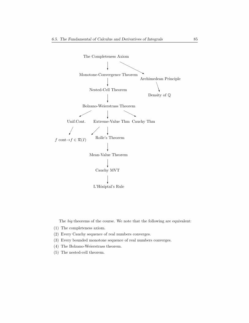
The big theorems of the course. We note that the following are equivalent:

(1) The completeness axiom.

(2) Every Cauchy sequence of real numbers converges.

(3) Every bounded monotone sequence of real numbers converges.

(4) The Bolzano-Weierstrass theorem.

(5) The nested-cell theorem.

86 6. Integration

6.6. Homework

Exercise 6.1. Let f(x) = c on [a, b]. Show f ∈ R[a, b] andR b

af(x) dx = c(b− a).

Exercise 6.2. Let

f(x) =

�

1 x = 00 x > 0

.

Show that f is Darboux integrable on [0, 1] and findR 1

0f(x)dx.

Exercise 6.3. Let

f(x) =

�

x x ∈ Q

0 x ∈ Qc

Show that f is not Darboux integrable on [0, 1].

Exercise 6.4.

f(x) =

1 0 ≤ x < 12 x = 1

−1 1 < x ≤ 2

Show that f is Darboux integrable on [0, 2] and findR 2

0f dx.

Exercise 6.5. (Thomae’s Function) Let

f(x) =

0 x ∈ Qc

1n x ∈ Q, x = m

n1 x = 0

Show that f is Darboux integrable on [0, 1].

Exercise 6.6. Show the functions in Problems (6.1), (6.2), and (6.4) are integrableby applying theorems.

Exercise 6.7. Give examples of functions f and g with fg and |f | integrable onsome bounded closed interval, but with neither f or g Darboux integrable on thatinterval.

Exercise 6.8. Give examples of a function f : [0, 1] → R and g : [0, 1] → R bothRiemann integrable on [0, 1] such that f ◦ g is not Riemann integrable on [0, 1]. Sof, g ∈ R[a, b] does not imply f ◦ g ∈ R[a, b]. Hint: look at Problem 4.7.

Exercise 6.9. Let a < c < b, and let f be defined on [a, b]. Show that f ∈ R[a, b]

if and only if f ∈ R[a, c] and f ∈ R[c, b]. Moreover,R b

af =

R c

af +

R b

cf .

Exercise 6.10. Suppose f ∈ R[a, b]. Show that

Z b

a

f = limc→a+

Z b

c

f .

Exercise 6.11. Suppose limkPk→0

S(f, P ) = I for some I ∈ R. Let {Pn}n∈N be any

sequence of partitions such that limn→∞

kPnk = 0. Show limn→∞

S(f, Pn) = I.

Exercise 6.12. Suppose f ∈ C[a, b] and f(x) ≥ 0 for all x ∈ [a, b] with f not

identically zero. Show thatR b

af > 0.

Exercise 6.13. Suppose f, g ∈ C[a, b] andR b

af =

R b

ag. Show that f(c) = g(c) for

some c ∈ [a, b]. (For fun can you supply a physical interpretation of this?)

6.6. Homework 87

Exercise 6.14. Suppose f ∈ C[a, b]. Show there is a c ∈ [a, b] such that

f(c) =1

b− a

Z b

a

f.

Exercise 6.15. (Mean-Value Theorem for Integrals) Generalize the previous prob-lem: Suppose f : [a, b] → R is continuous and g : [a, b] → R is integrable on [a, b]

withR b

a g 6= 0. Moreover, suppose g(x) ≥ 0 for all x ∈ [a, b]. Then, there existsc ∈ [a, b] such that

Z b

a

f(x)g(x) dx = f(c)

Z b

a

g(x) dx.

Exercise 6.16. Prove Theorem 6.28. That is, suppose f is bounded on [a, b] andf is Riemann integrable on every closed subinterval of (a, b), then f ∈ R[a, b]. Usethis to show the function

f(x) =

�

sin 1x 0 < x ≤ 1

0 x = 0

is Riemann integrable on [0, 1].

Exercise 6.17. Find with proof the following limits

(1) limn→∞

1

n

nX

i=1

i

n.

(2) limn→∞

nX

i=1

1

i+ 2n.

(3) limn→∞

1

n

nX

i=1

sin

�

iπ

2n

�

.

Exercise 6.18. We proved in Example 3.28 that the sequence

Sn =1

n+ 1+

1

n+ 2+ · · ·+ 1

2n

is monotone increasing and bounded above (you do not need to show this). Wewere not able to find the limit then - now we can. Find the limit (Hint: it is aRiemann sum).

Exercise 6.19. Define

lnx =

Z x

1

1

tdt

for x > 0. Prove that lnx is continuously differentiable and injective on (0,∞). Wedefine the number e so that ln e = 1. Prove that e exists. Also show that f(x) = ex

is the continuous inverse of lnx. You need only apply appropriate theorems for thisproblem.

Exercise 6.20. (integration by parts). Suppose u and v are differentiable functionson [a, b] and that both u′ and v′ are integrable on [a, b]. Show that both uv′ andu′v are Riemann integrable on [a, b]. Then prove that

Z b

a

uv′ = uv�

�

�

b

a−Z b

a

u′v.

88 6. Integration

Exercise 6.21. By considering the upper and lower sums forR n

1 lnx dx show

limn→∞

n!

nn= 0 and lim

n→∞(n!)1/n

n=

1

e.

Exercise 6.22. Suppose f ∈ C[a, b] andR x

af = 0 for all x ∈ [a, b]. Show f = 0 on

[a, b].

Exercise 6.23. Suppose f ∈ C[a, b] andR x

af =

R b

xf for all x ∈ [a, b]. Show f = 0

on [a, b].

Exercise 6.24. Suppose f ∈ C[a, b] and strictly positive on [a, b]. Show thatF (x) =

R x

a f is strictly increasing on [a, b].

Exercise 6.25. Computed

dx

Z x3

x2

cos(t2) dt.

Exercise 6.26. If f is Riemann integrable on [a, b], showR b

af dx = lim

c→a+

R b

cf dx.

Suppose f is given by

f(x) =

�

0 −1 ≤ x ≤ 01 0 < x ≤ 1

Compute F (x) =R x

−1f dx and F (1) using the fundamental theorem of calculus.

Recall f does not have an anti-derivative.

Exercise 6.27. Suppose f is continuous on [0, 1]. Define gn(x) = f(xn) for n ∈ N.Prove

that limn→∞

Z 1

0

gn(x) dx = f(0).

Exercise 6.28. We say a continuous function on R is periodic with period p > 0if f(x+ p) = f(x) for all x ∈ R. Show by example that antiderivatives of periodicfunctions need not be periodic while derivatives of continuously differentiable peri-odic function are always periodic. Prove that a necessary and sufficient conditionfor a periodic function to have periodic antiderivative is for f to have zero averageover one period. That is,

R p

0 f(t) dt = 0 is required.

Exercise 6.29. Let f be Riemann integrable on [−a, a], where a > 0. Prove thefollowing.

(a) If f is even, thenR a

−af dx = 2

R a

0f dx.

(b) If f is odd, thenR a

−a f dx = 0.

Exercise 6.30. Let f be continuous and nonnegative on [0, 1]. Define M =max{f(x)| x ∈ [0, 1]}. Show that

M = limn→∞

�Z 1

0

fn dx

�1/n

.

6.6. Homework 89

Exercise 6.31. Suppose f is continuous on [a, b] and thatZ b

a

f(x)ϕ(x) dx = 0

for all continuous ϕ on [a, b] with ϕ(a) = 0 = ϕ(b). Then f(x) = 0 on [a, b].

Exercise 6.32. Suppose f is continuous on [a, b] and thatZ b

a

f(x)ϕ′(x) dx = 0

for all continuously differentiable functions ϕ on [a, b] with ϕ(a) = 0 = ϕ(b). Thenf(x) is constant on [a, b].

Exercise 6.33. Suppose f : [a, b] → R is Riemann integrable on [a, b]. ShowF (x) =

R x

0f(t) dt satisfies the inequality |F (x)−F (y)| ≤ C|x− y| for all x ∈ [a, b].

Then show F is uniformly continuous on [a, b]. Calculate, justifying your steps,F (x) =

R x

0f(t) dt, where

f(t) =

�

0 0 ≤ t ≤ 11 1 < t ≤ 2

Exercise 6.34. Show

f(x) =

�

0 0 ≤ x ≤ 11 1 < x ≤ 2

is Riemann integrable on [0, 2], and find F (x) =R x

0f(t) dt. What properties does

F have?

Exercise 6.35. Clear up the devastating Example 1.2 in Chapter one. A functionf : [0,∞) → R is called uniformly Lipschitz - there exists M such that |f(x) −f(y)| ≤ M |x− y| for all x, y ∈ [0,∞). Now prove the following theorem.

Theorem Suppose f : [0,∞) → R is uniformly Lipschitz andZ ∞

0

|f(x)| dx < ∞.

Then limx→∞

|f(x)| = 0.

Prove the theorem by proving the contrapositive. That is, negate limx→∞

|f(x)| =0, use the properties of f to show

R∞0

|f(x)| dx = ∞.

Exercise 6.36. Repeat Problem 6.35 only assume f is differentiable on [0,∞) andZ ∞

0

(f ′(x))2 dx < ∞.