Integrating Concepts in Biology

PowerPoint Slides for Chapter 19:Emergent Properties at the Population Level

byA. Malcolm Campbell, Laurie J. Heyer, and

Chris Paradise

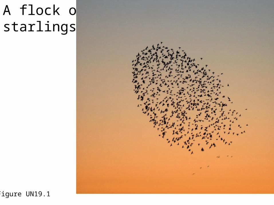
A flock of starlings

Figure UN19.1

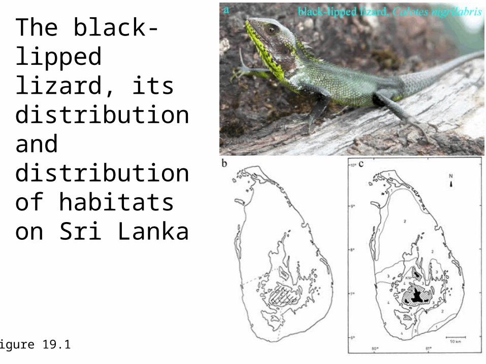
The black-lipped lizard, its distribution and distribution of habitats on Sri Lanka

Figure 19.1

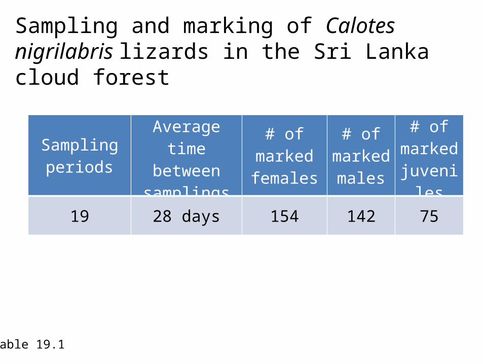
Sampling and marking of Calotes nigrilabris lizards in the Sri Lanka cloud forest

Table 19.1

Sampling periods

Average time between

samplings

# of marked females

# of marked males

# of marked

juveniles

19 28 days 154 142 75

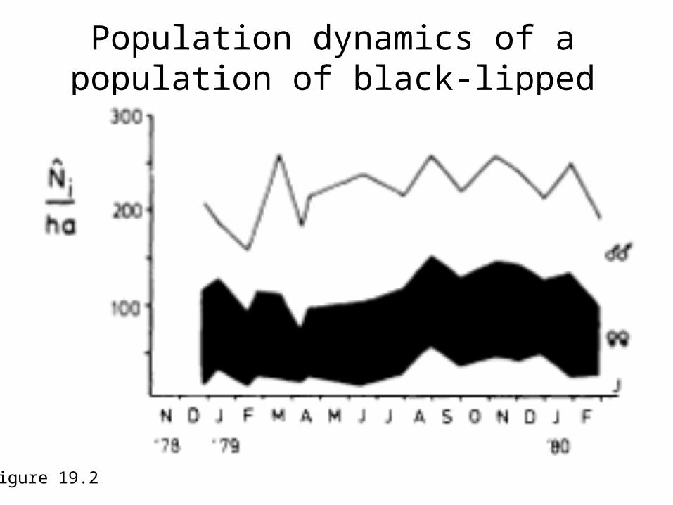
Population dynamics of a population of black-lipped lizards in Sri Lanka

Figure 19.2

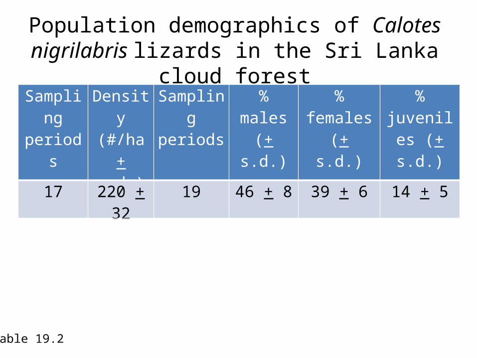
Population demographics of Calotes nigrilabris lizards in the Sri Lanka cloud forest

Table 19.2

Sampling periods

Density (#/ha +

s.d.)

Sampling periods

% males (+ s.d.)

% females (+ s.d.)

% juveniles (+ s.d.)

17 220 + 32 19 46 + 8 39 + 6 14 + 5

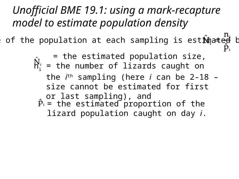
The size of the population at each sampling is estimated by

= the estimated population size, ni = the number of lizards caught on the ith sampling (here

i can be 2-18 – size cannot be estimated for first or last sampling), and

= the estimated proportion of the lizard population caught on day i.

Unofficial BME 19.1: using a mark-recapture model to estimate population density

Unofficial BME 19.1: using a mark-recapture model to estimate population density

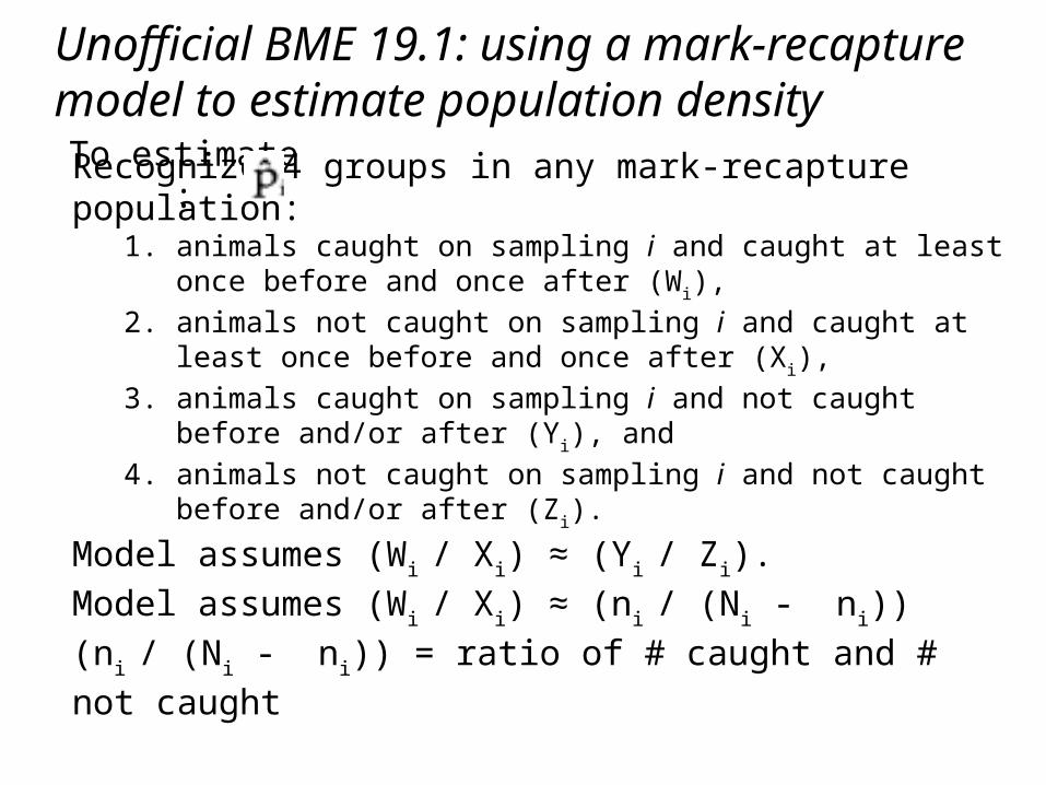
Recognize 4 groups in any mark-recapture population:1. animals caught on sampling i and caught at least once before and once

after (Wi),

2. animals not caught on sampling i and caught at least once before and once after (Xi),

3. animals caught on sampling i and not caught before and/or after (Yi),

and 4. animals not caught on sampling i and not caught before and/or after

(Zi).

Model assumes (Wi / Xi ) ≈ (Yi / Zi ).

Model assumes (Wi / Xi ) ≈ (ni / (Ni - ni))

(ni / (Ni - ni)) = ratio of # caught and # not caught

To estimate :

Unofficial BME 19.1: using a mark-recapture model to estimate population density

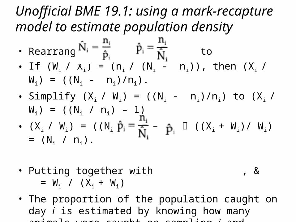
• Rearrange to

• If (Wi / Xi ) = (ni / (Ni - ni)), then (Xi / Wi ) = ((Ni - ni)/ni).

• Simplify (Xi / Wi ) = ((Ni - ni)/ni) to (Xi / Wi ) = ((Ni / ni) – 1)

• (Xi / Wi ) = ((Ni / ni) – 1) ((Xi + Wi )/ Wi ) = (Ni / ni).

• Putting together with , & = Wi / (Xi + Wi )

• The proportion of the population caught on day i is estimated by knowing how many animals were caught on sampling i and caught at least once before and once after (Wi), and how many animals were not caught on sampling i and caught at least once before and once after (Xi).

Unofficial BME 19.1: using a mark-recapture model to estimate population density

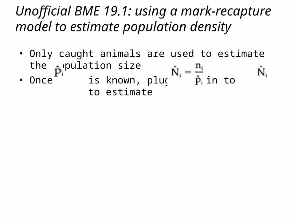
• Only caught animals are used to estimate the population size

• Once is known, plug back in to to estimate

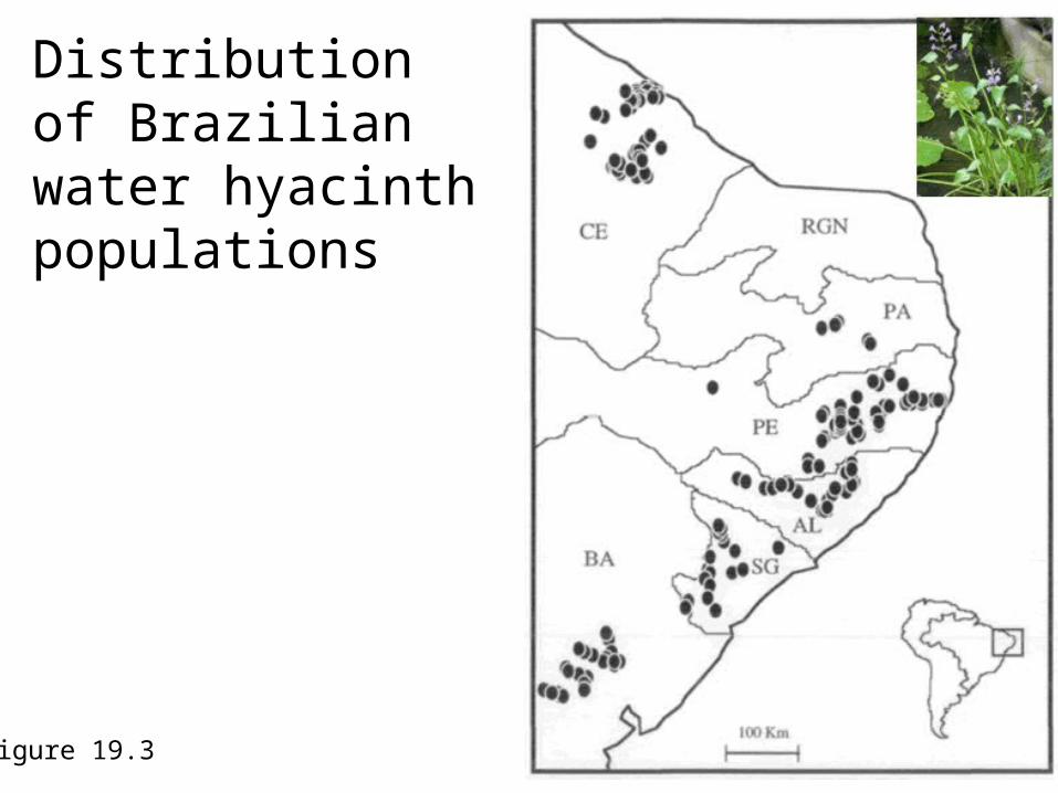
Distribution of Brazilian water hyacinth populations

Figure 19.3

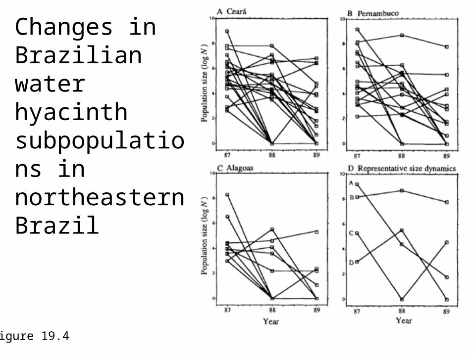
Changes in Brazilian water hyacinth subpopulations in northeastern Brazil

Figure 19.4

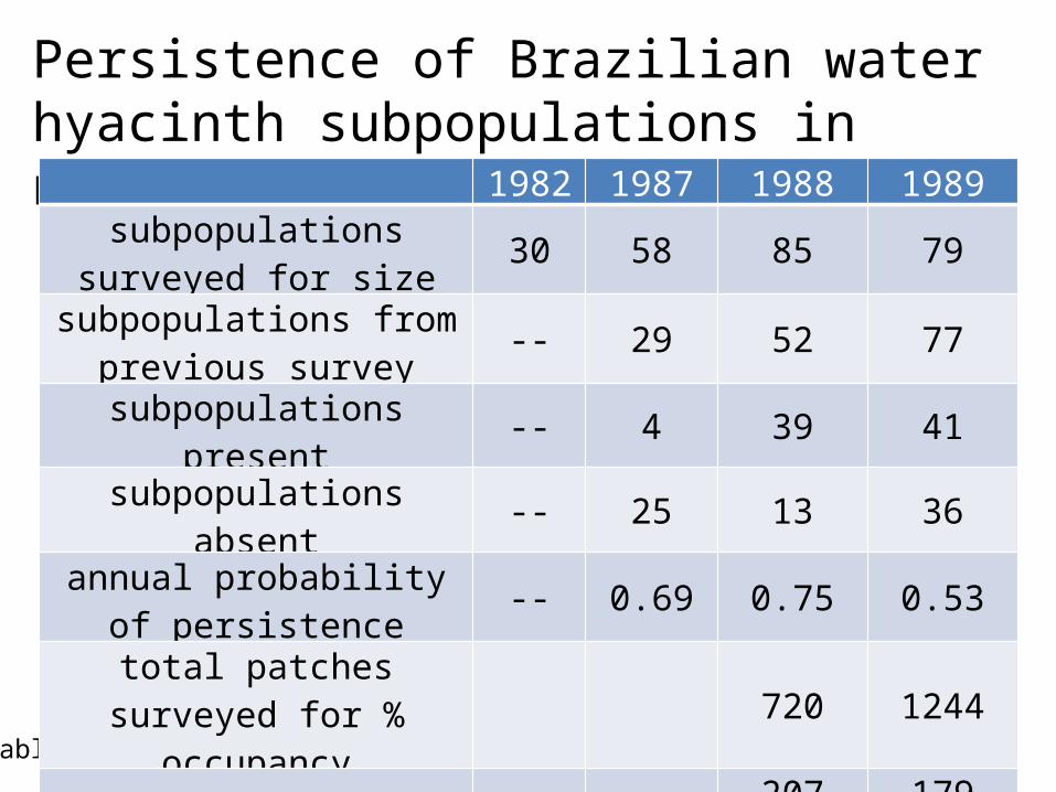
Persistence of Brazilian water hyacinth subpopulations in northeastern Brazil

Table 19.3

  1982 1987 1988 1989subpopulations surveyed for

size 30 58 85 79

subpopulations from previous survey -- 29 52 77

subpopulations present -- 4 39 41subpopulations absent -- 25 13 36annual probability of

persistence -- 0.69 0.75 0.53

total patches surveyed for % occupancy     720 1244

number (and %) of patches occupied     207

(28.8%)179

(14.4%)

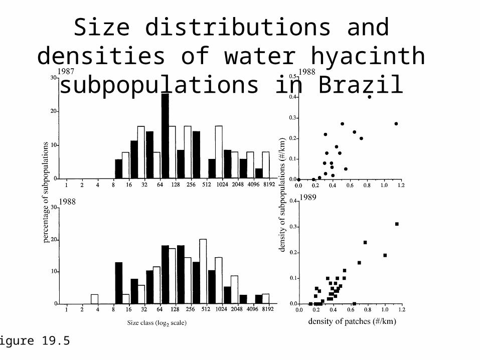
Size distributions and densities of water hyacinth subpopulations in Brazil

Figure 19.5

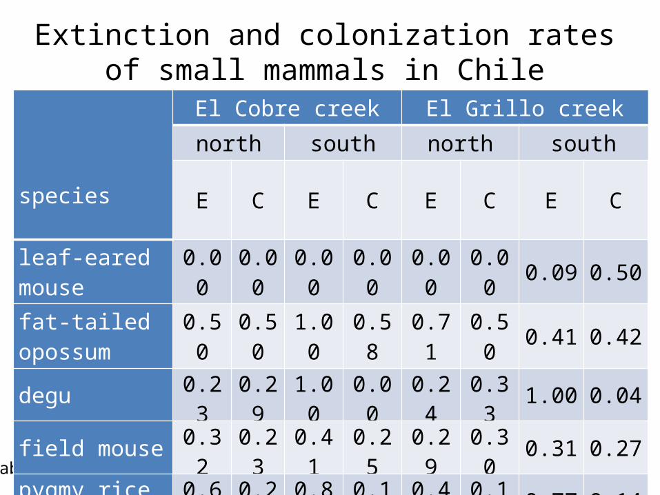
Extinction and colonization rates of small mammals in Chile

Table 19.4

  species

El Cobre creek El Grillo creek

north south north south

E C E C E C E C

leaf-eared mouse 0.00 0.00 0.00 0.00 0.00 0.00 0.09 0.50

fat-tailed opossum 0.50 0.50 1.00 0.58 0.71 0.50 0.41 0.42

degu 0.23 0.29 1.00 0.00 0.24 0.33 1.00 0.04

field mouse 0.32 0.23 0.41 0.25 0.29 0.30 0.31 0.27

pygmy rice rat 0.68 0.26 0.88 0.14 0.46 0.18 0.77 0.14

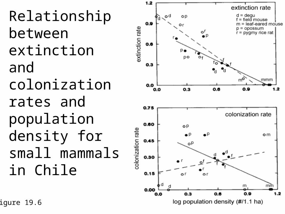
Relationship between extinction and colonization rates and population density for small mammals in Chile

Figure 19.6

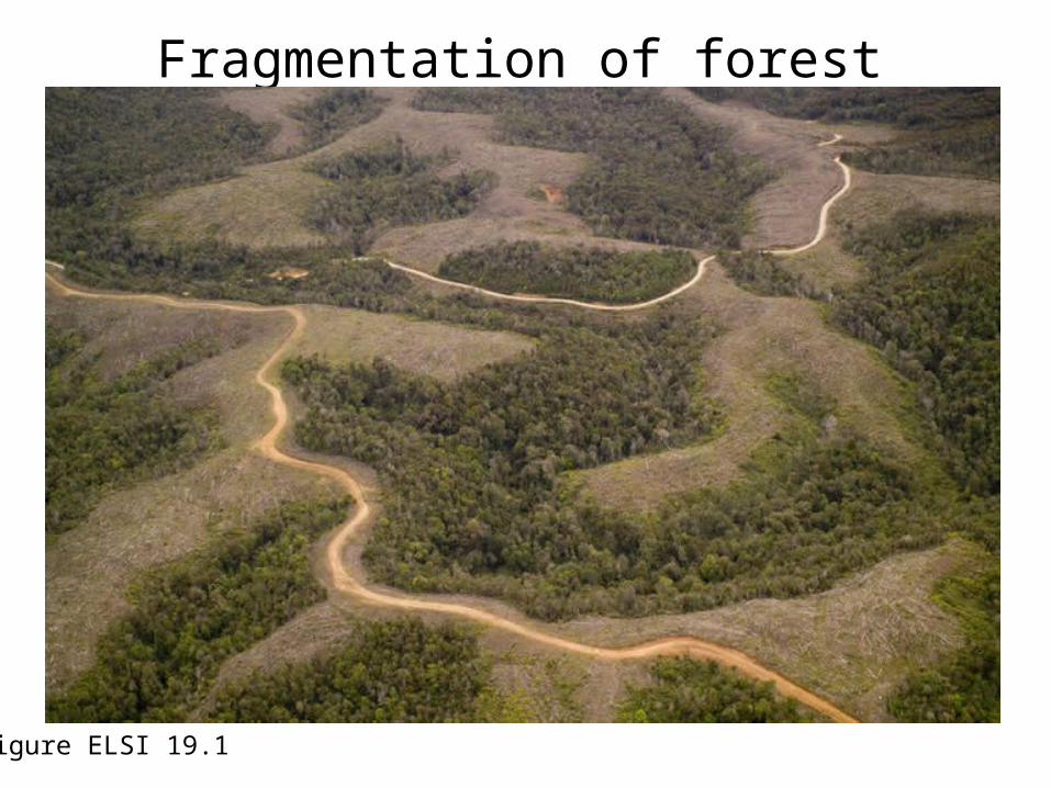
Fragmentation of forest hilltops in Chile

Figure ELSI 19.1

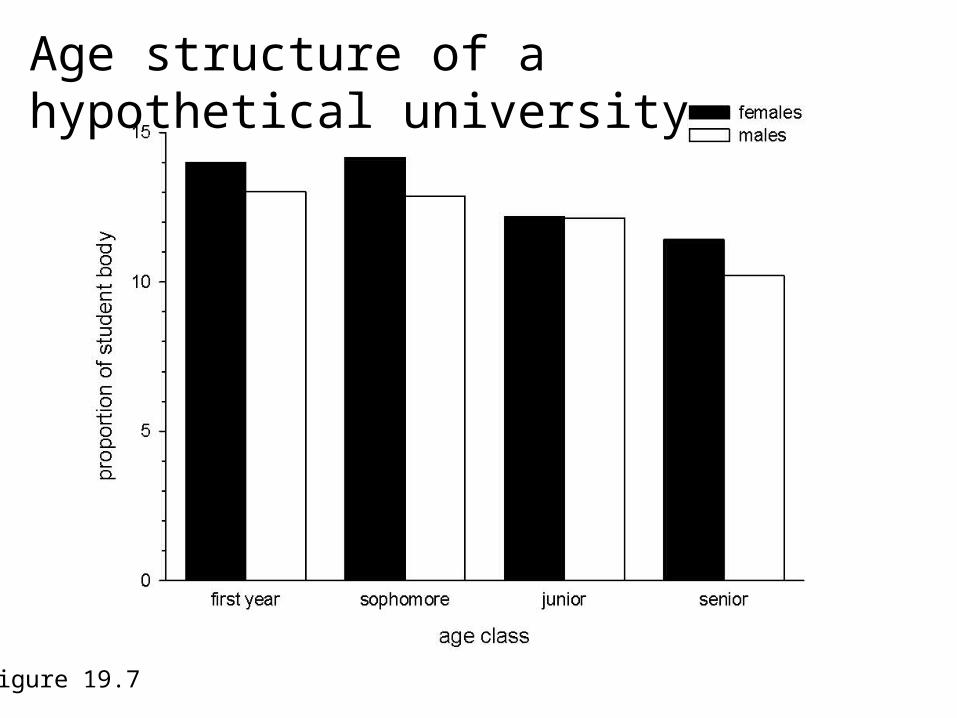
Age structure of a hypothetical university

Figure 19.7

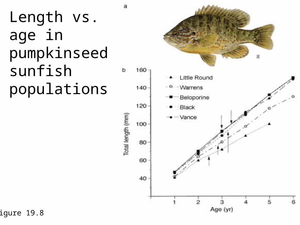
Length vs. age in pumpkinseed sunfish populations

Figure 19.8

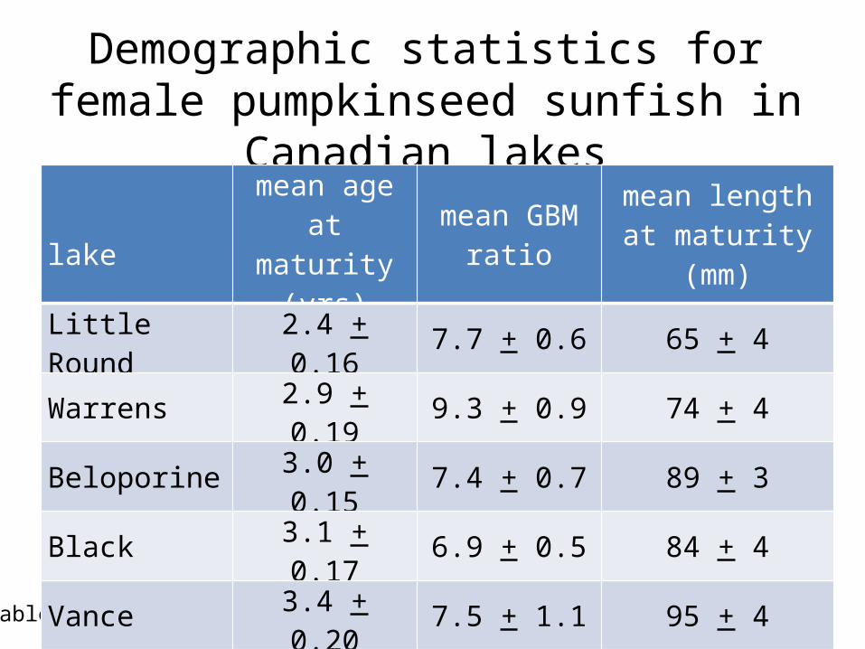
Demographic statistics for female pumpkinseed sunfish in Canadian lakes

Table 19.5

 lake

mean age at maturity (yrs)

mean GBM ratio

mean length at maturity (mm)

Little Round 2.4 + 0.16 7.7 + 0.6 65 + 4

Warrens 2.9 + 0.19 9.3 + 0.9 74 + 4

Beloporine 3.0 + 0.15 7.4 + 0.7 89 + 3

Black 3.1 + 0.17 6.9 + 0.5 84 + 4

Vance 3.4 + 0.20 7.5 + 1.1 95 + 4

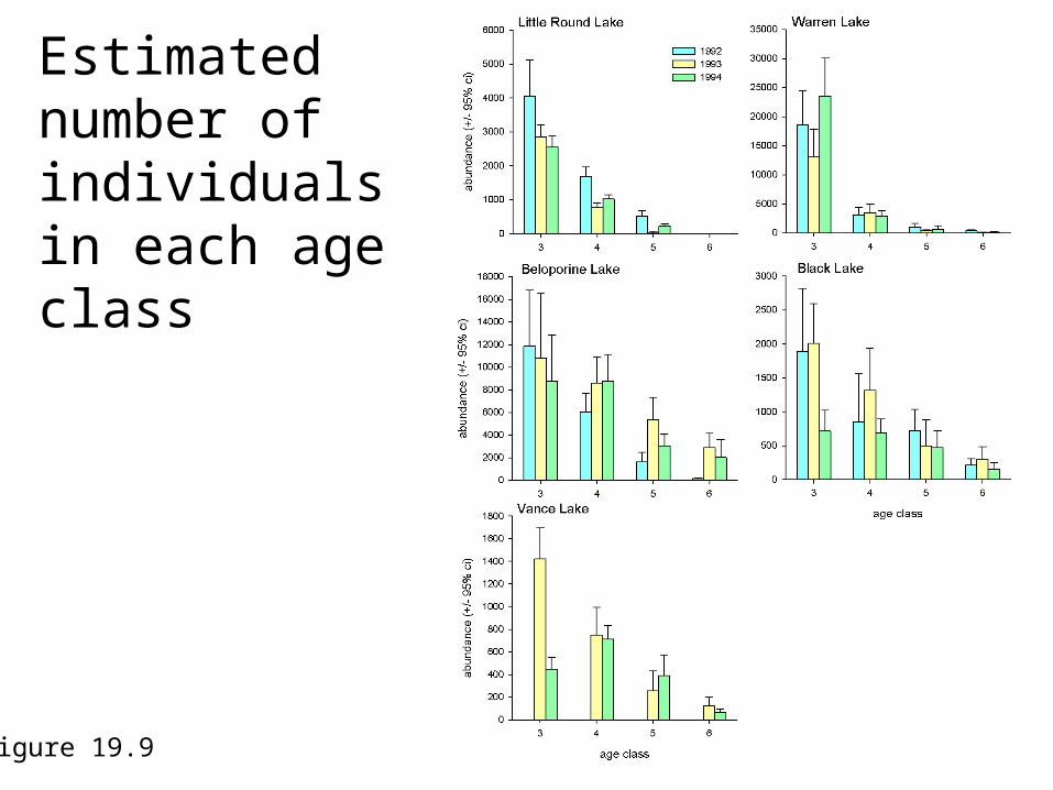
Estimated number of individuals in each age class

Figure 19.9

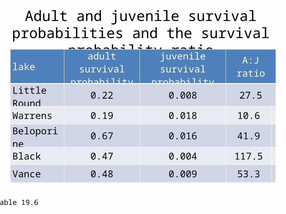
Adult and juvenile survival probabilities and the survival probability ratio

Table 19.6

lake adult survival probability

juvenile survival probability A:J ratio

Little Round 0.22 0.008 27.5

Warrens 0.19 0.018 10.6  

Beloporine 0.67 0.016 41.9  

Black 0.47 0.004 117.5  

Vance 0.48 0.009 53.3  

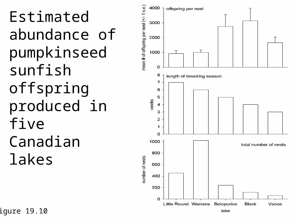
Estimated abundance of pumpkinseed sunfish offspring produced in five Canadian lakes

Figure 19.10

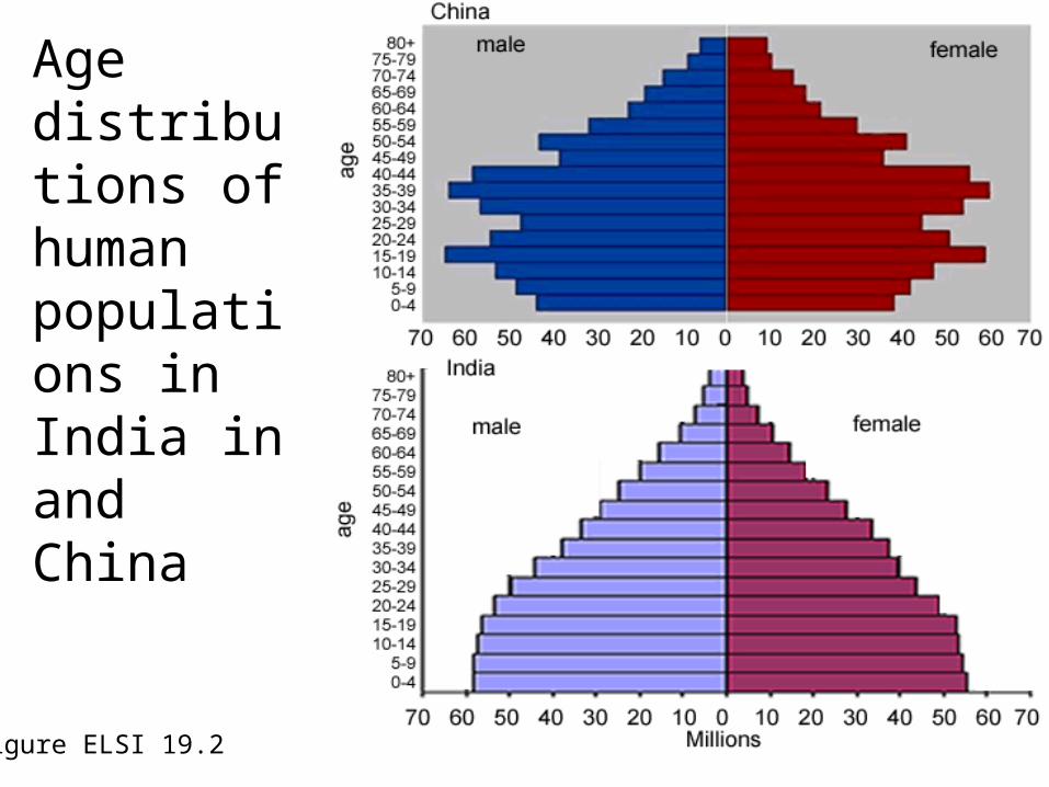
Age distributions of human populations in India in and China

Figure ELSI 19.2

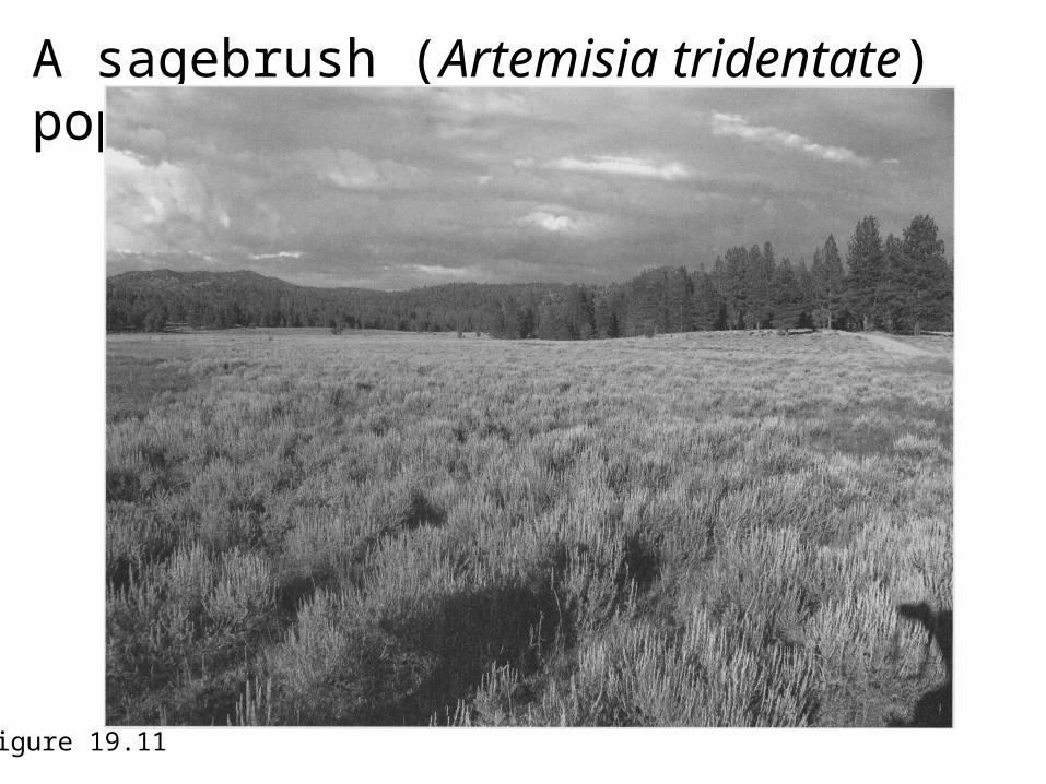
A sagebrush (Artemisia tridentate) population

Figure 19.11

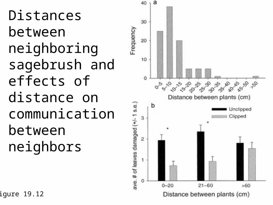
Distances between neighboring sagebrush and effects of distance on communication between neighbors

Figure 19.12

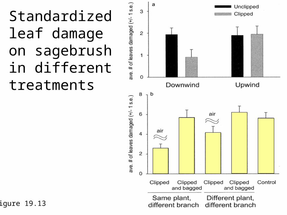
Standardized leaf damage on sagebrush in different treatments

Figure 19.13

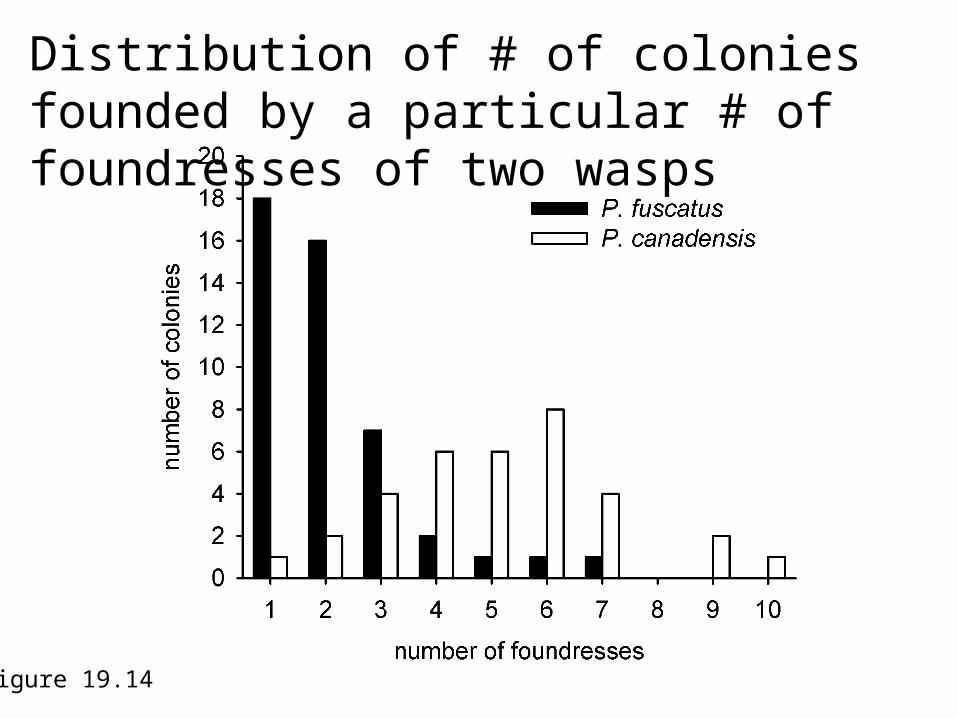
Distribution of # of colonies founded by a particular # of foundresses of two wasps

Figure 19.14

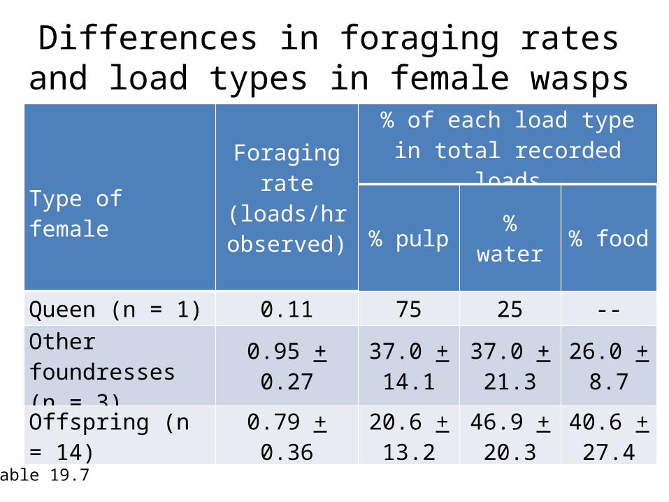
Differences in foraging rates and load types in female wasps

Table 19.7

 Type of female

Foraging rate (loads/hr observed)

% of each load type in total recorded loads

% pulp % water % food

Queen (n = 1) 0.11 75 25 --

Other foundresses (n = 3) 0.95 + 0.27 37.0 +

14.137.0 + 21.3

26.0 + 8.7

Offspring (n = 14) 0.79 + 0.36 20.6 + 13.2

46.9 + 20.3

40.6 + 27.4

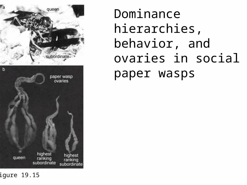
Dominance hierarchies, behavior, and ovaries in social paper wasps

Figure 19.15

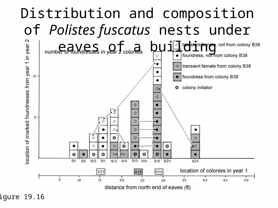
Distribution and composition of Polistes fuscatus nests under eaves of a building

Figure 19.16

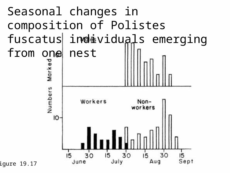
Seasonal changes in composition of Polistes fuscatus individuals emerging from one nest

Figure 19.17

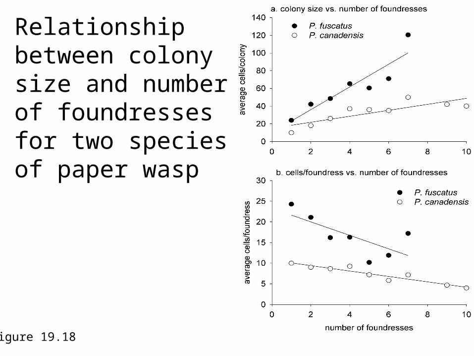
Relationship between colony size and number of foundresses for two species of paper wasp

Figure 19.18

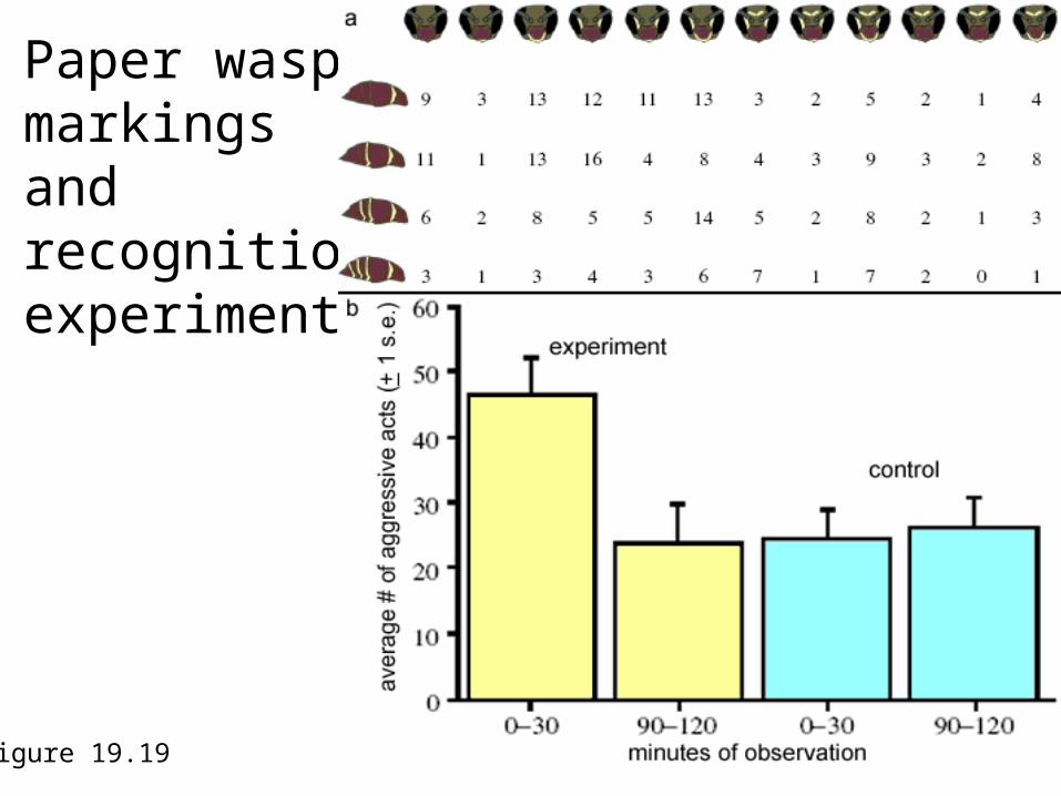
Paper wasp markings and recognition experiments

Figure 19.19

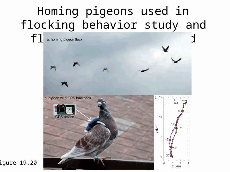
Homing pigeons used in flocking behavior study and flight path of displaced pigeons

Figure 19.20

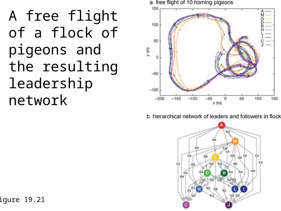
A free flight of a flock of pigeons and the resulting leadership network

Figure 19.21

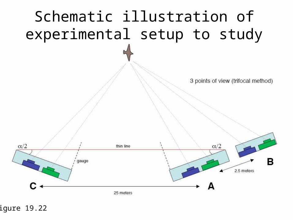
Schematic illustration of experimental setup to study starling flocks

Figure 19.22

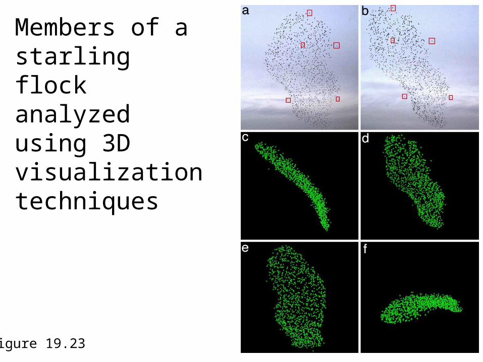
Members of a starling flock analyzed using 3D visualization techniques

Figure 19.23

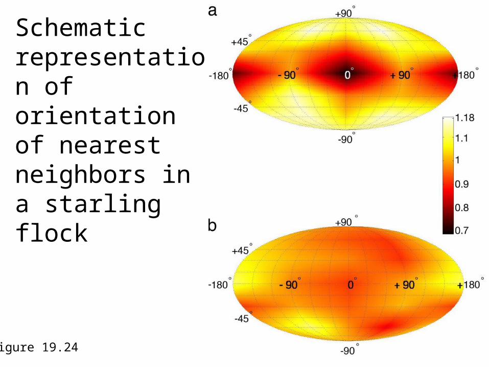
Schematic representation of orientation of nearest neighbors in a starling flock

Figure 19.24

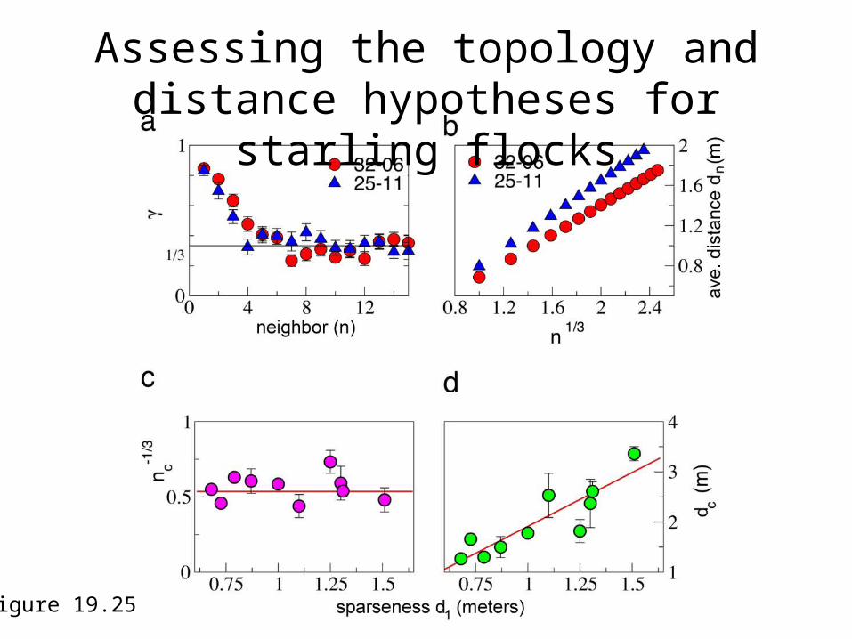
Assessing the topology and distance hypotheses for starling flocks

Figure 19.25

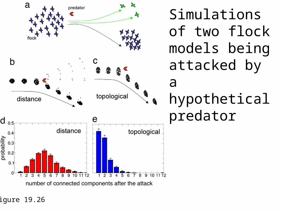
Simulations of two flock models being attacked by a hypothetical predator

Figure 19.26