Embed Size (px)
Citation preview

UNESCO-IHP Water Programme for Environmental Sustainability, Climate Change and Human Impacts
on the Sustainability of Groundwater Resources: Quantity and Quality Issues, Mitigation and Adaptation Strategies in Brazil
Integrated Environmental Assessment of
Agricultural and Farming Production Systems
in the Toledo River Basin (Brazil)
Pier Paolo Franzese, Otávio Cavalett, Tiina Häyhä, Salvatore D’Angelo

Published in 2013 by the United Nations Educational, Scientific and Cultural Organization
7, place de Fontenoy, 75352 Paris 07 SP, France
© UNESCO 2013 All rights reserved
ISBN 978-92-3-001138-3
The designations employed and the presentation of material throughout this publication do
not imply the expression of any opinion whatsoever on the part of UNESCO concerning the
legal status of any country, territory, city or area or of its authorities, or concerning the
delimitation of its frontiers or boundaries.
The ideas and opinions expressed in this publication are those of the authors; they are not
necessarily those of UNESCO and do not commit the Organization.
Cover design and illustrations: Pier Paolo Franzese
Printed by: UNESCO Printed in English

Table of contents
Background ....................................................................................................................... 1 Executive summary .......................................................................................................... 2 1. Introduction ................................................................................................................ 3
1.1 Toledo River Basin ................................................................................................. 4 1.2 Pig production system ............................................................................................ 5 1.3 Soybean-corn production system............................................................................ 8 1.4 Problems related to water use in the Toledo River basin ....................................... 9
2. Methodology .............................................................................................................. 10 2.1 Emergy Theory, Accounting and Evaluation Method .......................................... 11 2.2 Embodied Energy Analysis .................................................................................. 12 2.3 Material Flow Accounting .................................................................................... 13
2.4 Life Cycle Assessment ......................................................................................... 14 2.5 Ecological Footprint ............................................................................................. 15 2.6 Water Footprint .................................................................................................... 16
2.7 Carbon Footprint .................................................................................................. 18 2.8 System boundaries, functional units, and allocation ............................................ 19
3. Results and Discussion ............................................................................................. 20
3.1 Emergy Synthesis ................................................................................................. 20 3.2 Embodied Energy Analysis .................................................................................. 26
3.3 Material Flow Accounting .................................................................................... 28 3.4 Life Cycle Assessment ......................................................................................... 33
3.5 Ecological Footprint ............................................................................................. 38 3.6 Water Footprint .................................................................................................... 40
3.7 Carbon Footprint .................................................................................................. 44 3.8 Performance and sustainability indicators: scenario analysis .............................. 45
4. Conclusion ................................................................................................................. 53 Acknowledgements ........................................................................................................ 53
References ...................................................................................................................... 54 Annex 1: Calculation notes for corn production system. ............................................... 61
Annex 1a: Calculation notes for agricultural machinery in corn production ............. 64 Annex 1b: Local emissions in corn production .......................................................... 64
Annex 2: Calculation notes for soybean production system .......................................... 65
Annex 2a: Calculation notes for agricultural machinery in soybean production ....... 67 Annex 2b: Local emissions in soybean production .................................................... 68
Annex 3: Calculation notes for pig production system .................................................. 69 Annex 3a: Parameters for pig production ................................................................... 70 Annex 3b: Local emissions from manure management in the pig production ........... 70
Authors' biographical sketch...........................................................................................71

1
Background
Brazil has plenty of water resources but they are unevenly distributed across the
country. In this context, groundwater plays a crucial role supplying towns, industries,
and agricultural and farming systems. Climate variability and change as well as human
activities could significantly impact Brazilian groundwater resources. The IPCC
scenarios for temperature and rainfall in Brazil for the next 20-50 years show a
significant warming across the country and a possible reduction of annual rainfall in
portions of the north-eastern region and in the Amazon. In addition, there are risks of
overexploitation and contamination of groundwater resources in vulnerable agricultural
areas. The evaluation of these impacts and the definition of appropriate mitigation and
adaptation measures are therefore much needed.
To address these issues, a UNESCO-IHP project involving Brazilian and Italian
institutions was carried out. The main goals of the project entitled “UNESCO-IHP
Water Programme for Environmental Sustainability, Climate Change and Human
Impacts on the Sustainability of Groundwater Resources: Quantity and Quality Issues,
Mitigation and Adaptation Strategies in Brazil” were: (a) to understand the hydrologic
relationships between control and response variables in groundwater systems under the
impact of climate change and human activities; (b) to identify mitigation and adaptation
measures for groundwater management under those impacts; (c) to evaluate
hydrological adaptive and mitigation measures in terms of replicability, sustainability,
impacts of both global and regional climate change, and equality in access to
groundwater, both in quantitative and qualitative terms.
In this context, the present study aimed at performing an integrated environmental
assessment of agricultural and farming production systems located in the Toledo River
Basin (Paraná State, Brazil). Water, material, energy, and money resources invested in
supporting such production systems were evaluated with the final goal of calculating a
large set of multi-criteria indicators useful to describe the environmental performance
and sustainability of the production systems at farm and basin level. Finally, three
alternative scenarios were drawn to explore the sustainable use of resources according
to different land uses, production levels, and management practices, paying special
attention to water use.

2
Executive summary
In this study, the environmental performance and sustainability of soybean-corn
intercrop and pig production systems in the Toledo River basin (Brazil) were explored.
The main steps of the study were: (a) identification of the spatial and temporal
boundaries of the investigated systems; (b) modeling of the selected agricultural and
farming production systems by means of H.T. Odum’s energy-symbolic language; (c)
inventory of the main water, mass, energy, and money input flows to the production
systems; (d) conversion of the quantified input flows by means of appropriate intensity
factors according to different environmental assessment methods; (e) calculation of
mass, water, energy, and emergy performance indicators at farm level; (f) calculation of
ecological, water and carbon footprints generated by the investigated production
processes; (g) upscaling of up-stream and down-stream indicators of environmental
impacts and sustainability at basin level; (h) calculation of indicators of environmental
performance and sustainability for three alternative scenarios at basin level.
An integrated assessment framework was implemented by using the following methods:
Emergy Synthesis, Embodied Energy Analysis, Material Flow Accounting, Life Cycle
Assessment, Ecological Footprint, Water Footprint, and Carbon Footprint.
The multi-criteria approach used in this study provided useful information about the
interactions and use of natural capital, human-driven resources, and ecosystem services
supporting agricultural and farming production systems in the Toledo River basin
(Brazil). The outcomes of the study will support local managers and policy makers
committed to develop management schemes and environmental policies based on the
sustainable management of agroecosystems. In addition, the results of the study will
provide a useful benchmark for future investigations.
All indicators were calculated at farm scale and then upscaled to basin level to assess
the environmental load of alternative scenarios at regional level. The indicators of
environmental performance highlighted the intensification process occurring in the
basin over the last decades. The indicators of environmental sustainability showed an
increased dependence on non-renewable resources (mainly imported from outside the
region) supporting the intensive agricultural and farming systems located in the Toledo
River basin. The scenario analysis showed the environmental support and impacts for
three alternative options in terms of land use, production levels, and management
practices. The assumptions made in Scenario A pointed out a possible reduction of the
environmental impacts in the basin. The use of water, the manure concentration as well
as the interaction between the increasing impact of human-dominated production
activities and the effects of climate change in the region are also discussed in the study.

3
1. Introduction
The Toledo River basin is located in the south-western portion of the state of Paraná and
has an area of about 92 km2 (Winter et al., 2005). Underlain by the Guarani aquifer, the
Toledo River basin has a very high potential for groundwater use. The basin is
characterized by intensive agricultural and farming production processes, among which
the most important are soybean-corn and pig production systems. Most of the manure
produced by pig production systems is used to fertilize soil with little or no treatment.
Such a practice generates a set of environmental impacts due to the excess of manure
produced in this region. Soybean-corn production systems are frequently fertilized with
manure and they represent an important cropping system in the Toledo River basin.
These crops are also related to the pollution of groundwater due to a massive use of
agrochemicals. Moreover, the lower reach of the Toledo River crosses the urban area of
the city of Toledo that is experiencing a fast population growth. Both agricultural and
farming production systems are related to a massive use of groundwater and water
pollution phenomena. Over time, the cumulative application of manure and
agrochemicals as well as the urban sprawl can lead to severe groundwater pollution.
In this study, energy, material and water requirements of a selected farm integrating
corn-soybean and pig production in Toledo River basin were assessed implementing the
following steps:
1. Identification of the spatial and temporal boundaries of the investigated systems;
2. Modeling of the selected agricultural and farming production systems by means
of Odum’s energy-symbolic language;
3. Inventory of the main water, mass, energy, and money input flows;
4. Conversion of the quantified input flows by using appropriate intensity factors
according to different environmental assessment methods;
5. Calculation of mass, water, energy and emergy performance indicators at farm
level;
6. Calculation of ecological, water, and carbon footprints generated by the
investigated production processes;
7. Upscaling of up-stream and down-stream indicators of environmental impacts
and sustainability at basin level;
8. Calculation of indicators of environmental performance and sustainability for
alternative scenarios at basin level.
The integrated assessment framework was implemented by using the following
methods: Emergy Synthesis, Embodied Energy Analysis, Material Flow Accounting,
Life Cycle Assessment, Ecological Footprint, Water Footprint, and Carbon Footprint.

4
This framework provided a set of indicators able to describe the environmental
performance and sustainability of the investigated systems in terms of yield, resource
use and efficiency, local versus imported resource use, renewable versus non-renewable
resource use, environmental load, sustainability, interaction with and dependence on
local environment, and intensity of water and land use.
Indicators calculated at farm scale were upscaled to basin level to assess the impacts of
alternative scenarios at regional level. Special attention was paid to water use
supporting agricultural and farming production systems. The relationship between the
increasing impact of human-dominated activities and climate change are also discussed
in the study.
1.1 Toledo River Basin
The Toledo River basin is located in the south-western portion of the state of Paraná,
covering an area ranging from 24°43' to 24°47' South latitude and from 53°33' to 53°45'
West longitude. The Toledo River has a length of about 27 km and it is the most
important river of the town of Toledo. Its water represents an important resource,
exploited to supply 40% of the population of the town of Toledo (Winter et al., 2005;
Tomm, 2001).
The Toledo River basin is a sub-basin of the São Francisco Verdadeiro River and it is
part of the larger Paraná III hydrographic basin. The Toledo River basin accounts for
only 4.2% of the area of Paraná state but it is considered to play an important role, also
because of its contribution to the reservoir of the Itaipu Binacional dam. Moreover, the
Toledo River basin is underlain by the Guarani aquifer, showing a very high potential
for groundwater use. The multiple use of water in this area can cause conflict between
energy generation, farming systems, agricultural activities and urban sprawl (PNMA II,
2002).
The area of the Toledo River basin is about 9,290 ha and it has a population of
approximately 550 inhabitants. The basin comprises 195 farms, of which 47 include pig
production activities (Winter et al., 2005). The soybean-corn production is very
important for the local economy but it also contributes to water pollution problems due
to the high use of agrochemicals. The population of Toledo municipality is 116,774
inhabitants while the total cropped area covers about 75,000 ha (IBGE, 2009). The local
economy is based on agriculture and livestock farming. The main crops are: soybean,
wheat, corn, beans, rice, cassava, castor bean, peanut, cotton, sugarcane, and tobacco.
The main livestock products are poultry and pork (Tomm, 2001).

5
The total area cropped with soybean in Toledo municipality covers 65,300 ha with a
harvest of 206,634 tons of soybeans in 2008 (IBGE, 2009). Figure 1 shows an example
of cropping system integrated with several pig farms (stables) located very close to the
Toledo River basin.
Figure 1. Aerial photography showing cropping systems integrated with pig farms located very close to
the Toledo River basin. (Source: Google Maps).
1.2 Pig production system
Pig production is an important economic activity in Brazil with a herd of 35 million
heads, representing the fourth largest producer worldwide (3 million tons per year), the
fourth largest exporter (600,000 tons per year), and the sixth largest consumer (11-13 kg
inhabitant-1
year-1
). Pig production is mainly concentrated in the southern part of Brazil
(IBGE, 2006; Miele and Waquil, 2007).
Pig production has dramatically changed in the last three decades, shifting from a small-
subsistence model to a larger number of intensive farming systems. This trend towards
industrial feeding operations has been driven by the reduction of production and logistic
costs for both farmers and meat processors (Kunz et al., 2009; FAO, 2006). However,
this model is causing several environmental problems associated with a higher

6
concentration of animals as well as a higher dependence on external resources (Cavalett
et al., 2006, 2010). An additional trend in meat production is the migration of
production operations from developed to developing countries, basically due to: lower
operating costs, greater availability of feed, land, and water as well as less restrictive
environmental policies in comparison to Europe (EU-nitrate directive) or USA (EPA–
CAFO rules) (Kunz et al., 2009; FAO, 2005).
In Brazil, effluent disposal in superficial waters is covered by federal regulations
(CONAMA, 2005) which are very restrictive for animal wastewater. However, the
regulation for effluents disposal through land applications is more flexible and differs
according to different regions. At present, there is no regulation for water reuse.
Around 12,000 pig producers are located in the Parana III hydrographic basin. They
produce 1.4 million animals, with 6,000 heads butchered per day (PNMA II, 2002). The
Toledo River basin hosts 47 farms producing about 11,000 pig heads per year. Such an
amount of pigs produces approximately 150,000 liters of manure per day (Winter et al.,
2005). An average pig produces a daily amount of manure equivalent to about 10
human beings. This way, the pig population of the basin has an impact in terms of
manure production equivalent to a population of 110,000 inhabitants, while the actual
population of the basin accounts for only 550 inhabitants. Figure 2 shows a picture of a
pig production system located in the Toledo river basin.
Figure 2. Pig production system located in the study area of the Toledo River basin
(Source: Parthenope University of Naples, Italy).

7
The storage of liquid manure and its application to soil is the predominant manure
management practice in Brazil and other countries. This is due to simplicity and low
management cost as well as the possible reduction of the costs related to the
replacement of chemical fertilizers by manure nutrients (Kunz et al., 2009). The main
disadvantage of land manure application is the fact that manure transportation is not
economically viable for distances beyond a few kilometers (Seganfredo and Girotto,
2004).
Taking into consideration the UN recommendation of manure spread of 170 kg of
nitrogen per hectare per year (European Council Regulation, 1999), in the Toledo basin
it would be necessary to have about 780 ha to dispose of the produced manure avoiding
environmental problems. This figure highlights the problem of lack of available land for
manure spread since 72% of the farms located in the basin have less than 20 ha of land
(Winter et al., 2005). Moreover, according to the Brazilian Forestall Law, all the farms
in this area of Brazil must preserve at least 20% of the area with original forest. The
resulting lack of available land determines the accumulation of manure in soil and water
with the related environmental problems. In the Toledo River basin 84% of farms have
a creek, 63% have spring water, and 47% have some area with original forest. The
riparian forest accounts for about 4% of the basin area (Tomm, 2001).
There is a set of potential environmental impacts involved in pig production due to its
rapid expansion. These impacts (increasing atmospheric emissions of ammonia, nitrous
oxide and methane as well as decrease in water quality) can be noted in all segments of
the supply chain, from grain and animal production to processing, distribution and
consumption. Because of the large amount of waste generated by pig production and its
impact on air, soil, and water resources, animal production has been highly debated by
both local and regional governments (Kunz et al., 2009; Sharpley et al., 2002; Pereira et
al., 2008).
The effects of manure on water are caused by the excess of nitrogen and phosphorus.
The effects on air are due to toxic gas emissions (ammonia, nitrous oxide, and methane)
and unpleasant odors to human population. There are also negative influences caused by
intensive pig production on animal and vegetal biodiversity (Pereira et al., 2008). In
addition, because of the great variety of soils, plant fertilizer requirements, agronomic
practices and manure composition, land application of manure has shown the potential
to promote an imbalance in soil-plant nutrient absorption capacity (Seganfredo, 1999).
The intensification of pig production in recent decades by using less area and specific
diets is based on the massive use of fossil energy in all production processes such as
installations, feed, medicaments, and transport. The huge concentration of pig farms in

8
some areas, together with coal extraction and the wide use of agrochemical, has created
a severe threat to the Guarani aquifer, the biggest water source of South America
(Pinheiro Machado Filho et al., 2001).
The inadequate management of pig manure can also contribute to raising emissions in
the atmosphere. For example, each molecule of N2O has a potential contribution to
global warming effects equivalent to 296 molecules of CO2 (IPCC, 2006). Another
crucial issue related to pig production is the direct and indirect use of water. For
instance, according to a conservative estimation, at least 3.5 liters of water are needed
per pig per day only as cleaning water (Pinheiro Machado Filho et al., 2001).
1.3 Soybean-corn production system
In the past three decades soybean has become one of the main agricultural commodities
in Brazil. Next to the United States, Brazil is the second largest producer and exporter
of soybean worldwide (FAO, 2007). The National Supply Company (CONAB)
estimated Brazil’s harvest to be approximately 57.1 million tons in 2008/09. During this
harvest period about 21.7 million hectares were cultivated for soybean production in the
whole country (CONAB, 2009), a land area equal to the size of Great Britain.
The rapid expansion of soybean production in Brazil has been stimulated mainly by the
industrial demand for a cheap, high-protein ingredient for animal feed in Brazil and
Europe. About 80% of the soybean produced worldwide is used by livestock industry
(Gelder and Dros, 2005). The grain is used to supply intensive meat and dairy
production, feeding the ever-growing demand for cheap meat. The animal feed industry
is expecting an average increase in world consumption of meat from 38.2 kg per capita
per year in 2005 to 42.6 kg by 2020 (Gomes et al., 2008).
Soybean is a very important crop in the Toledo region. In 2008, the area cultivated with
soybean in the Toledo region was 65,300 ha with a harvest of 206,634 tons of soybean
(IBGE, 2009). Soybean is produced in the region during the summer season while corn
and wheat are cultivated in the same area in the other seasons. Corn is a feed for pig
production while soybean is mostly sold to the market or exchanged with soybean
crusher for soy meal to be used as a pig feed ingredient. Intensive agricultural practices
for soybean production rely on direct and indirect use of fossil fuels (diesel, machinery,
fertilizers, and agrochemicals). The massive use of non-renewable resources generates
high pressure on the local agroecosystem, jeopardizing the sustainability of soybean
production (Pengue, 2005; Ortega at al., 2005; Cavalett and Ortega, 2009).

9
Figure 3 shows the soybean and corn production systems located in the study area of
Toledo River basin.
Figure 3. Soybean (a) and corn (b) field in the study area of Toledo River basin
(Source: Parthenope University of Naples, Italy).
1.4 Problems related to water use in the Toledo River basin
In recent years, several interruptions to the water supply occurred in the town of Toledo
because of the low water quality caused by pig manure pollution. The chemical
pollution in the Toledo River (mainly due to widespread use of agrochemicals) also
caused some interruptions in the water supply to the population of the town of Toledo
(Nieweglowski, 2006).
The Rio Sao Francisco Verdadeiro hydrographic basin (which includes the Toledo
River as a sub-basin) has been cited as the most polluted among those debouching into
the reservoir of the Iguaçu dam. This basin pollutes the lake of the Iguaçu dam with up
to 60,000 tons of sediment per year (Nieweglowski, 2006).
a b

10
2. Methodology
Sustainability can be analyzed from an environmental, social or economic perspective.
Moreover, sustainability can be assessed at different scales. At each scale, specific
questions can be posed. Natural and human economies are self-organizing systems,
where processes are linked and therefore affect each other at multiple scales.
Investigating the behavior of a single process and merely seeking the maximization of
only one parameter (energy efficiency, production cost, jobs, etc.) is unlikely to provide
sufficient insights to properly inform policy making. Instead, several methods can be
selected and applied at different scales by developing an integrated assessment
framework. Each method can supply a piece of information about system performance
at an appropriate scale, highlighting different perspectives and concerns complementary
to each other. Integration supplies a deeper understanding of the overall picture and it is
characterized by an “added value” that could not be achieved by means of a single
crtiterion approach. The choice of a proper set of methods is therefore of crucial
importance (Buonocore et al., 2012; Häyhä et al., 2011; Ulgiati et al., 2006; 2010).
The rationale underlying different methodologies for evaluating resource production
and consumption as well as the need for integration of different approaches towards a
comprehensive assessment framework was discussed by Ulgiati et al. (2006; 2008;
2011a,b). In this study an integrated assessment framework was implemented by using
the following methods: a) Emergy Synthesis, b) Embodied Energy Analysis, c) Material
Flow Accounting, d) Life Cycle Assessment, e) Ecological Footprint, f) Water
Footprint, and g) Carbon Footprint. The selected methods have different scientific
backgrounds and frames of attention and they account for the direct and indirect
environmental support required to generate and make available natural and human-
driven resources invested in the production process under investigation.
In this study, the investigated systems were treated as a “black box” and an inventory of
all the input and output flows was firstly performed on its local scale. This inventory
formed a common basis for all subsequent assessments carried out in parallel to ensure
the maximum consistency of basic assumptions and input data (Annexes 1, 2, and 3).
The outcome of such an integrated assessment framework was a set of multi-criteria
indicators calculated at multiple scales and describing different aspects of the system
performance and sustainability as well as different environmental problems and
concerns.
Evaluating alternative scenarios, regarding different possible uses of natural and
economic resources, necessarily requires the adoption of a multi-criteria approach.
There is no single “optimal” solution to all problems. Only an assessment based on
11
several complementary methods can highlight the inevitable trade-offs characterizing
alternative scenarios, thus enabling a wiser selection of the option embodying the best
compromise in light of the existing economic, social, technological, and environmental
conditions.
In the next paragraphs we provide a brief description of each evaluation method used in
this study.
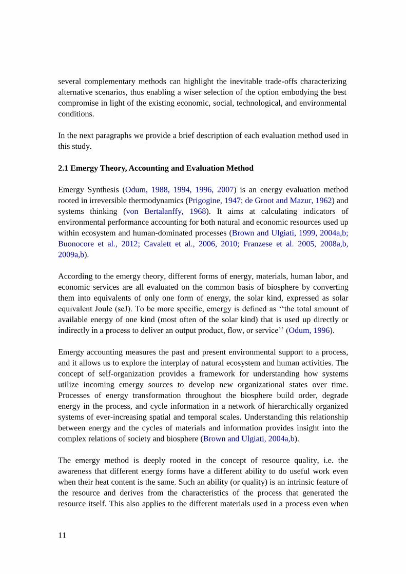
2.1 Emergy Theory, Accounting and Evaluation Method
Emergy Synthesis (Odum, 1988, 1994, 1996, 2007) is an energy evaluation method
rooted in irreversible thermodynamics (Prigogine, 1947; de Groot and Mazur, 1962) and
systems thinking (von Bertalanffy, 1968). It aims at calculating indicators of
environmental performance accounting for both natural and economic resources used up
within ecosystem and human-dominated processes (Brown and Ulgiati, 1999, 2004a,b;
Buonocore et al., 2012; Cavalett et al., 2006, 2010; Franzese et al. 2005, 2008a,b,
2009a,b).
According to the emergy theory, different forms of energy, materials, human labor, and
economic services are all evaluated on the common basis of biosphere by converting
them into equivalents of only one form of energy, the solar kind, expressed as solar
equivalent Joule (seJ). To be more specific, emergy is defined as ‘‘the total amount of
available energy of one kind (most often of the solar kind) that is used up directly or
indirectly in a process to deliver an output product, flow, or service’’ (Odum, 1996).
Emergy accounting measures the past and present environmental support to a process,
and it allows us to explore the interplay of natural ecosystem and human activities. The
concept of self-organization provides a framework for understanding how systems
utilize incoming emergy sources to develop new organizational states over time.
Processes of energy transformation throughout the biosphere build order, degrade
energy in the process, and cycle information in a network of hierarchically organized
systems of ever-increasing spatial and temporal scales. Understanding this relationship
between energy and the cycles of materials and information provides insight into the
complex relations of society and biosphere (Brown and Ulgiati, 2004a,b).
The emergy method is deeply rooted in the concept of resource quality, i.e. the
awareness that different energy forms have a different ability to do useful work even
when their heat content is the same. Such an ability (or quality) is an intrinsic feature of
the resource and derives from the characteristics of the process that generated the
resource itself. This also applies to the different materials used in a process even when

12
their masses are the same. The quality of a resource depends on its physical-chemical
characteristics, which in turn depend on the work performed by nature to make it via the
complex pattern of natural process. Instead of only looking at what can be extracted
from a resource (exergy), the emergy evaluation method focuses on what it takes for
biosphere to make and for societies to process a given resource. Odum (1988, 1994,
1996) pointed out that in all systems a greater amount of low-quality energy must be
dissipated in order to generate a product containing a smaller amount of higher energy
quality, thus generating an energy-based hierarchy of resources and products. The ratio
of the available energy previously used up to make a product to the actual energy
content of such a product provides a measure of the hierarchical position of the item
within the thermodynamic scale of the biosphere (a kind of production cost of the item
measured in ‘‘biosphere currency’’). Such a ratio is expressed as solar equivalent Joules
per Joule (seJ J-1
) or per gram (seJ g-1
), termed transformity and specific emergy,
respectively. The more energy previously used up, the higher the product’s
transformity, and the product therefore corresponds to a higher position in the energy
hierarchy (Odum, 1996). Insofar as natural or economic dynamics select the optimum
process capable of generating a given product, the amount of required input emergy
decreases to the minimum emergy demand for its production. According to such a
selection driven perspective, transformity translates into an energy scaling ratio to
indicate quality and hierarchical position of different resources in the hierarchy of
biosphere.
Other emergy indicators and ratios can be calculated to evaluate the use of resources in
production processes. For example, the Renewability index (%R) is the percentage of
renewable emergy used by the system; the Emergy Yield Ratio (EYR) is the ratio
between the total emergy inflow and the emergy purchased from outside the system; the
Environmental Loading Ratio (ELR) is the ratio between imported plus local non-
renewable emergy and the local renewable one; the Empower Density (ED) is the ratio
between the total input emergy and the area of investigation over time. Odum (1996)
and Brown and Ulgiati (2004b) provided a detailed explanation of the emergy
accounting procedures for a variety of systems as well as a careful discussion about the
meaning of the emergy-based indicators. The updated emergy baseline for biosphere of
15.83∙1024
seJ yr-1
(Brown and Ulgiati, 2004b) was used in this study and all the emergy
intensity factors (specific emergy and solar transformity factors) were updated to this
baseline.
2.2 Embodied Energy Analysis
Total input heat flow must always be equal to total output heat flow for isothermal
systems, according to the First Law of Thermodynamics. Environmental as well as

13
economic concerns may motivate us to investigate the consequences of releasing into
the environment a resource characterized by a higher temperature than the
environmental temperature. To address these aspects, a careful description and
quantification of input and output heat flows is needed. However, it must be
remembered that the energy invested in the overall production process is no longer
available to the final user of the product as it has been used up and is no longer
contained in the final product. The actual energy content of the product (measured as
combustion enthalpy, HHV, LHV) differs from the total input energy because of the
losses in all steps of the production processes leading to the final product (Ulgiati et al.,
2003).
The Embodied Energy Analysis (EEA) has been defined as the process of determining
the energy required directly and indirectly to allow a system to produce a product or
service (IFIAS, 1974). The Gross Energy Requirement (GER) method accounts for the
amount of fossil energy (also referred to as commercial energy) required directly and
indirectly to make a good or service (Slesser, 1978; Smil, 1991; Herendeen, 1998;
Franzese et al., 2009b). The GER method is concerned with the depletion of fossil fuels
and it focuses on the availability and use of fossil and fossil-equivalent energy invested
to produce a product or service. Direct use of fossil fuels refers to oil, lubricants, and
electricity, while indirect use of fossil fuels is related to structures, machinery,
fertilizers, pesticides, and chemicals, among others.
In the GER method, all inputs to the process are multiplied by an energy intensity factor
accounting for the amount of fossil resources directly and indirectly required to make
them available. The total of such fossil and fossil-equivalent energy requirement
represents the GER of the process while the ratio between the GER of the process and
the amount of generated product provides the GER of the product (usually expressed in
MJ per kg). Renewable resources provided for free by nature (without using any fossil
energy to make them available) are not accounted for by the GER method. Human labor
and economic services are also not included in most GER evaluations (Franzese et al.,
2009b).
2.3 Material Flow Accounting
The Material Flow Accounting (MFA) method (Schmidt-Bleek, 1993; Hinterberger and
Stiller, 1998) is aimed at evaluating the environmental disturbance associated with the
withdrawal or diversion of material flows from their natural ecosystemic pathways.
When expanding the scale of investigation, we realize that each flow of matter supplied
to a process has been extracted and processed elsewhere. Additional matter is moved
from place to place, processed and then disposed of to supply each input to the process.

14
Sometimes a huge amount of rock must be excavated per unit of metal or chemical
element actually delivered to the final user. Most of this rock is then returned to the
mine site, but its stability is lost and several chemical compounds become soluble with
rainfall, thus affecting the environment in unexpected ways. There are therefore two
main aspects of the material balance to be considered: 1) when addressing the input
side, we must account for the total input mass supporting a process, thus indirectly
measuring how the process affects the environment by withdrawing resources (Bargigli
et al., 2005); and 2) when focusing on the product side, we must be sure that
economically and environmentally significant matter flows have not been neglected.
In this method, appropriate material intensity factors (kg unit-1
) are multiplied by each
input to the process, accounting for the total amount of abiotic matter, biotic matter,
water, and air directly or indirectly required to make each input available to the process.
The resulting material demands of the individual inputs are then added up for each
environmental compartment (biotic and abiotic matter, water, and air), and assigned to
the system’s output as a quantitative measure of its cumulative environmental burden
from that compartment (often referred to as “Ecological Rucksack”).
2.4 Life Cycle Assessment
Life Cycle Assessment (LCA) is used worldwide to assess material and energy flows to
and from a production process. LCA is a method for determining the environmental
impacts of a product or service during its entire life cycle or, as in the case of this study,
from production of raw material inputs to their use in the agricultural/farming
production systems. LCA is a cooperative effort performed by many investigators
throughout the world (many working in the industrial sectors) to follow the fate of
resources from initial extraction and processing of raw materials to final disposal. This
effort is converging towards standard procedures and common frameworks to allow a
consistent comparison of final results. The International Standard Office provided a
very detailed investigation procedure for environmental management based on LCA and
for a comparable quality assessment (ISO 14040, 2006; ISO 14044, 2006). The
approach used in this study follows the ISO 14040-14044 standards and the current state
of the art of LCA methodology.
A typical LCA study consists of the following stages: (1) goal and scope definition; (2)
detailed life cycle inventory (LCI) analysis with compilation of data on energy and
resource use and emissions in the environment throughout the life cycle; (3) assessment
of the potential impacts related to the quantified forms of resource use and
environmental emissions; (4) interpretation of the results from the previous phases of

15
the analysis in relation to the objectives of the study (ISO 14040, 2006; ISO 14044,
2006).
In this study, the software package SimaPro® (PRé Consultants B.V.) and CML 2
Baseline 2000 v2.05 method were used for the environmental impact assessment of
corn, soybean, and pig production systems. The following environmental impact
categories were evaluated: Abiotic depletion (ADP); Acidification (AP);
Eutrophication (EP); Global warming potential (GWP); Ozone layer depletion (ODP);
Human toxicity (HTP); Fresh water aquatic ecotoxicity (FWAET); Marine aquatic
ecotoxicity (MAET); Terrestrial ecotoxicity (TET); and Photochemical oxidation
(POP).
2.5 Ecological Footprint
The Ecological Footprint methodology was developed in the early 1990s by the
academics Mathis Wackernagel and William Rees in Canada (Wackernagel and Rees,
1996). The Ecological Footprint (EF) is an accounting tool based on two fundamental
concepts: sustainability and carrying capacity. This method makes possible an
estimation of resource consumption and waste assimilation for a given population in
terms of equivalent productive land area. Since the land area owned or controlled by a
population is usually a limited and identifiable quantity, it can be compared to its actual
EF. This method can be applied to people, populations, products, firms, regions or
countries.
The difference between the available land and the actual EF, termed “ecological
deficit”, shows the dependence of a population on natural capital and ecosystem
services purchased from outside the area. The rationale for representing impacts upon
the environment in units of area is that biologically productive land area produces or
absorbs flows of several materials utilized by our society. The different uses of land
areas are often mutually exclusive and are therefore in competition for the finite area of
productive land in the world.
The EF combines several environmental impacts into a single area measure.
Conceptually, EF can include biological and energy resources, pollution, land use,
waste disposal, and provision of natural habitats. EF does not seek to include social
issues such as income distribution, education and criminality, nor economic issues such
as inflation, GDP, and unemployment. EF is therefore not a comprehensive measure of
sustainable development as it only includes a limited range of environmental concerns.
There are six classes of land usually considered for EF calculation: 1) crop; 2) carbon
dioxide absorption; 3) building area; 4) fishing; 5) grazing; and 6) forest.

16
In this study, the area used to produce 1 kg of output (crop land class) was added to the
area necessary to absorb the CO2 equivalent (CO2 absorption land class) due to the use
of the inputs (from the LCA). The cumulative area requirement of the system’s output
was then computed as the ecological footprint of the output measured in global hectares
(gha).
2.6 Water Footprint
The Water Footprint (WF), introduced in 2002, is a young concept and water footprint
assessment is a method still under development. The water footprint is an indicator of
freshwater use that looks at both direct and indirect water use. The water footprint can
be regarded as a comprehensive indicator of freshwater resources appropriation, next to
the traditional and restricted measure of water withdrawal. The water footprint of a
product is the volume of direct and indirect freshwater used to produce the product,
measured over the full supply chain. It is a multi-dimensional indicator, showing water
consumption volumes by source and polluted volumes by type of pollution. All
components of the total water footprint are specified geographically and temporally.
Blue water footprint refers to consumption of blue water resources (surface and ground
water) along the supply chain of a product. “Consumption” refers to loss of water from
the available ground-surface water body in a catchment area, which happens when
water evaporates, returns to another catchment area or to the sea, or it is incorporated
into a product. Green water footprint refers to consumption of green water resources
(rainwater stored in soil as soil moisture). Grey water footprint refers to pollution and is
defined as the volume of freshwater required to assimilate the load of pollutants based
on existing ambient water quality standards (Hoekstra et al., 2009).
The water footprint method has been used in several studies, for instance in the “Value
of Water Research Report Series” published by the UNESCO-IHE Institute for Water
Education (Delft, the Netherlands) in collaboration with the University of Twente
(Enschede, the Netherlands), and Delft University of Technology (Delft, the
Netherlands) (Mekonnen and Hoekstra, 2010; Aldaya and Hoekstra, 2009; Aldaya and
Llamas, 2008; Bulsink et al., 2009; Hoekstra, 2008; Gerbens-Leenes et al., 2008a,b).
Since, in this study, special attention was paid to water resources use, the Water
Footprint method was applied to evaluate water resources use in corn, soybean, and pig
production systems in the Toledo River basin. Proper information about water footprints
of communities and businesses can help to understand how a more sustainable and
equitable use of fresh water resources can be achieved. The Water Footprint thus offers
a wider perspective on how a consumer or producer relates to the use of freshwater. WF

17
is a volumetric measure of water consumption and pollution. WF is not a measure of the
severity of local environmental impact by water consumption and pollution. The local
environmental impact of a certain amount of water consumption and pollution depends
on the vulnerability of the local water system, and on the number of water consumers
and polluters that are supplied by the same system. Water footprint accounts give
spatiotemporally explicit information on how water is appropriated for various human
purposes, thus also informing the discussion about sustainable and equitable water use.
Blue water resources are generally scarcer and have higher opportunity cost than green
water, thus suggesting a main focus on accounting for blue water footprint only. On the
other hand, green water resources are also limited and thus scarce, giving a reason for
accounting for green water footprint as well. Besides, green water can be substituted by
blue water and sometimes – particularly in agriculture – the other way around as well,
so that a complete picture can be obtained only by accounting for both of them. The
argument for including green water use is that the historical engineering focus on blue
water has led to the undervaluation of green water as an important production factor
(Hoekstra et al., 2009). The idea of calculating the grey water footprint was introduced
to express water pollution in terms of a polluted volume, so that it can be compared with
water consumption, also expressed as a volume (Hoekstra et al., 2009). If one is
interested in water pollution and in comparing the relative claims of water pollution and
water consumption on the available water resources, it is relevant to take into account
the grey footprint in addition to the blue water footprint.
The blue water footprint is an indicator of consumption of blue water, i.e. fresh surface
or groundwater. The term “consumptive water use” refers to one of the following three
cases: (a) water evaporates; (b) water is incorporated into the product, and (c) water
does not return to the same catchment area (e.g., it is returned to another catchment area
or to the sea) or in the same period (e.g., it is withdrawn in a scarce period and returned
in a wet period).
The green water footprint is the volume of rainwater consumed during the production
process. This is particularly relevant for agricultural and forestry products (products
based on crops or wood), where it refers to the total rainwater evapotranspiration (from
fields and plantations) plus the water incorporated into the harvested crop or wood.
The grey water footprint of a process is an indicator of the degree of freshwater
pollution that can be associated with the process. It is defined as the volume of
freshwater that is required to assimilate the load of pollutants based on existing ambient
water quality standards. Accordingly, it is calculated as the volume of water that is
required to dilute pollutants to such an extent that the quality of the ambient water

18
remains above agreed water quality standards. When a waste flow deals with more than
one form of pollution, as it is generally the case, the grey water footprint is determined
by the pollutant that is the most critical: i.e., the one that is associated with the largest
pollutant-specific grey water footprint. For the purpose of finding an overall indicator of
water pollution, the grey water footprint based on the critical substance is sufficient.
Water footprint studies highlight two aspects of water resources management. First, data
on water footprints of products, consumers, and producers inform the discourse about
sustainable, equitable, and efficient freshwater use and allocation. Freshwater is scarce;
its annual availability is limited. It is relevant to know who receives which portion and
how water is allocated over various purposes. For example, rainwater used for
bioenergy cannot be utilized for food production. Second, water footprint accounts help
to estimate environmental, social, and economic impacts at local and catchment level.
Environmental impact assessment should include a comparison of each water footprint
component to available water at relevant locations and time (accounting for
environmental water requirements).
The water footprint was calculated in this study using the methodology described in
Hoekstra et al. (2009). Hoekstra et al. (2009) points out that frameworks like MFA and
LCA consider the use of various types of environmental resources and look at different
types of impacts on the environment. In contrast, ecological footprint, water footprint,
and embodied energy analyses take the perspective of one particular resource or impact.
In this study we have implemented and applied an extended LCA assessment,
integrating different footprints and evaluation methods in a consistent conceptual
analytical framework.
2.7 Carbon Footprint
The Carbon Footprint is a subset of the Ecological Footprint and of the more
comprehensive Life Cycle Assessment (LCA). The Carbon Footprint is the measure of
the amount of greenhouse gases, measured in units of carbon dioxide, produced by
human activities. Carbon Footprint can be measured for an organization, event, product
or person, and is usually expressed in tons (or kg) of CO2 equivalents per kg of product.
The Carbon Footprint can be broken down into primary and secondary footprint. The
primary footprint is the sum of direct emissions of greenhouse gases from burning fossil
fuels for energy consumption and transportation. The secondary footprint is the sum of
indirect emissions of greenhouse gases generated during the life cycle of the production
process.

19
In this study, the Carbon Footprints of corn, soybean and pig production systems were
calculated as the category “Global Warming Potential” (GWP). Both primary and
secondary Carbon footprints were also considered in the LCA.
2.8 System boundaries, functional units, and allocation
System boundaries, defined as cradle-to-gate, include raw materials and emissions of
crop cultivation and pig production.
Functional units were defined as 1 kg of corn, 1 kg of soybean and 1 kg of live pig
meat. The main inputs and outputs of the soybean-corn intercrop production system
were accounted for 1 ha of an average farm located in the Toledo basin (Annexes 1 and
2). In the same way, the main inputs and outputs of the pig production system were
accounted for an average pig farm located in the Toledo River basin and producing 650
pig heads per year. The farmed animals are usually delivered to the processing industry
with an average weight of 110 kg after 120 days in the rearing system (Annex 3). Inputs
and outputs were referred to 1 kg of live pig meat produced.
According to LCA methodology, allocation is required for multi-product processes.
Other methods, such as material flow accounting, embodied energy analysis and
ecological footprint, also require allocation procedures. In this study, the criterion of
economic allocation based on the market value of the process output was applied, as
suggested in the ISO 14040-14044 documents for LCA (ISO 14040, 2006; ISO 14044,
2006). However, even if the co-products (corn stover, soybean straw, and pig manure)
play an important role within the integrated farm, no environmental impacts were
allocated to these co-products since they do not have any economic (market) value.
Delimitations of the study:
Materials and energy used in farm buildings construction were excluded from
this study.
Production, use, and emissions from vaccines and other pig medicines were not
considered in this study due to lack of knowledge about the environmental
impacts of these chemicals.
Disinfectants, washing detergents, and other minor stable inputs were also not
taken into account.
The components of pig feed indicated as other minerals corresponding to 3% (in
mass) were considered as salt (NaCl) or generic chemicals (in LCA) because of
simplification and lack of data for several specific components of this fraction:
salt, natural and synthetic amino acids, limestone, enzymes, phosphate, soy oil,
mix of vitamins, and mix of micronutrients.

20
3. Results and Discussion
The main water, material, energy, and money flows required by an average farm
integrating corn, soybean and pig production were evaluated by developing an
integrated environmental assessment framework. The data used to implement the
inventory of the production systems (Annexes 1, 2, and 3) were obtained from field
interviews to farmers, literature review and statistical books. Statistical data have been
checked against those obtained from interviews with farmers during the field work.
Input raw amounts (inventory), presented in Annex 1, 2, and 3, were multiplied by
suitable intensity factors specific to different evaluation methods and converted into
water, mass, energy, money and emergy units to account for their total (direct and
indirect) amounts. Finally, indicators of environmental performance (intensity factors)
and sustainability were calculated for the investigated processes. The set of multi-
criteria indicators was calculated at farm level and then upscaled to basin level to assess
the environmental impacts of alternative scenarios at regional scale. The results
obtained by using different assessment methods are presented in the following
paragraphs.
3.1 Emergy Synthesis
Figure 4 shows the energy systems diagram drawn to model the investigated systems.
Such a symbolic model, drawn according to a standardized energy systems language
(Odum, 1996), was used as a basis to develop the quantitative inventory of input and
output flows. The symbolic model shows in a pictorial way the system boundary, main
driving forces, producers, consumers, storages, and interactions among the system’s
components. According to Odum (1996), driving forces and system’s components were
drawn from left to right in order of increasing energy quality (i.e., increasing
transformity) to provide a reference to the energy hierarchy characterizing the
investigated systems.
Based on the systems diagram, input flows supporting agricultural and farming
production systems were identified, quantified, and converted to emergy units by means
of suitable emergy intensity factors. Finally, a set of emergy-based indicators were
calculated to explore the environmental performance and sustainability of the
investigated production activities.

21
Renewable
resources
$
Farmer
Agro-
chemicals
Soybean
Corn/
Wheat
Biodiv.
Original
forest
FishLake
Nutrients
River/
Creek
Farm
assets
Ground
water
Fertilizers DieselOther
materialsFeed Services
Biomass
Swine
Manure
Env.
services
Corn/wheat
Soybean
Manure
Swine
$
$
$
Figure 4. Energy systems diagram of a typical farm in the Toledo River basin (Brazil) integrating swine
and soybean-corn production systems.
The input emergy flows invested to support the production systems were assessed by
multiplying the raw data input flows by their specific emergy intensity factors (obtained
from literature after an accurate evaluation of their conformity to the investigated
process). Then, the emergy flows to the process (renewable and non-renewable
resources from nature, purchased resources from outside the system, labor and services
from human economy) were added to account for the total emergy supporting the
process over the spatial and temporal frame of investigation. Finally, several emergy-
based indicators for each production system were calculated. Tables 1, 2, and 3 show
the emergy evaluation for corn, soybean, and pig production systems, respectively.

22
Table 1. Emergy evaluation of the corn production system.
Note Description of flow Flow Unit ha-1 yr-1 Emergy intensity (seJ unit-1)
Reference for emergy intensities
Emergy (seJ ha-1 yr-1)
1 Sunlight 5.77E+13 J 1.00E+00 By definition 5.77E+13
2 Rain 5.52E+10 J 3.06E+04 Brown and Ulgiati, 2004b 1.69E+15
3 Deep heat 1.00E+10 J 1.02E+04 Odum, 1996 1.02E+14
4 Topsoil loss 4.07E+09 J 1.24E+05 Brown and Ulgiati, 2004b 5.05E+14
5 Limestone 2.14E+08 J 2.72E+06 Brown and Ulgiati, 2004b 5.82E+14
6 Agrochemicals 1.02E+01 kg 2.49E+13 Brown and Ulgiati, 2004b 2.53E+14
7 Seeds 1.79E+01 kg 1.15E+12 This study 2.05E+13
8 Organic fertilizer 1.03E+03 kg 1.13E+11 Castellini et al., 2006 1.17E+14
9 Nitrogen fertilizer 8.16E+01 kg 6.38E+12 Brown and Ulgiati, 2004b 5.21E+14
10 Phosphorus fertilizer 6.40E+01 kg 6.55E+12 Brown and Ulgiati, 2004b 4.19E+14
11 Potassium fertilizer 1.27E+02 kg 2.92E+12 Brown and Ulgiati, 2004b 3.71E+14
12 Fuel 2.14E+09 J 1.11E+05 Brown and Ulgiati, 2004b 2.36E+14
13 Machinery (steel) 2.85E+00 kg 1.13E+13 Brown and Ulgiati, 2004b 3.22E+13
14 Local labor 9.50E+00 USD 3.70E+12 Coelho et al., 1999 3.51E+13
15 Services 8.21E+02 USD 3.70E+12 Coelho et al., 1999 3.04E+15
Output
16 Corn 6.90E+03 kg 1.15E+12 This study 7.92E+15*
1.13E+11 J 7.00E+04 This study 7.92E+15
*According to emergy algebra the total input emergy was accounted for by avoiding double counting
among the renewable emergy flows.
Results in Table 1 show that the main emergy flows contributing to corn production
system were Services from human economy (38% of the total emergy input), chemical
potential of rain (21%), and limestone (7%).
Table 2. Emergy evaluation of the soybean production system.
Note Description of flow Flow Unit ha-1 yr-1 Emergy intensity (seJ unit-1)
Reference for emergy intensities
Emergy (seJ ha-1 yr-1)
1 Sunlight 5.77E+13 J 1.00E+00 By definition 5.77E+13
2 Rain 5.52E+10 J 3.06E+04 Brown and Ulgiati, 2004b 1.69E+15
3 Deep heat 1.00E+10 J 1.02E+04 Odum, 1996 1.02E+14
4 Topsoil loss 4.61E+09 J 1.24E+05 Brown and Ulgiati, 2004b 5.72E+14
5 Limestone 1.22E+08 J 2.72E+06 Brown and Ulgiati, 2004b 3.32E+14
6 Agrochemicals 1.05E+01 kg 2.49E+13 Brown and Ulgiati, 2004b 2.60E+14
7 Seeds 6.50E+01 kg 2.06E+12 This study 1.34E+14
8 Organic fertilizer 1.03E+03 kg 1.13E+11 Castellini et al., 2006 1.17E+14
9 Nitrogen fertilizer 0.00E+00 kg 6.38E+12 Brown and Ulgiati, 2004b 0.00E+00
10 Phosphorus fertilizer 6.00E+01 kg 6.55E+12 Brown and Ulgiati, 2004b 3.93E+14
11 Potassium fertilizer 6.00E+01 kg 2.92E+12 Brown and Ulgiati, 2004b 1.75E+14
12 Fuel 1.85E+09 J 1.11E+05 Brown and Ulgiati, 2004b 2.05E+14
13 Machinery (steel) 2.50E+00 kg 1.13E+13 Brown and Ulgiati, 2004b 2.83E+13
14 Local labor 9.18E+00 USD 3.70E+12 Coelho et al., 1999 3.40E+13
15 Services 5.80E+02 USD 3.70E+12 Coelho et al., 1999 2.15E+15
Output
16 Soybean 3.00E+03 kg 2.06E+12 This study 6.19E+15*
5.96E+10 J 1.04E+05 This study 6.19E+15
*According to emergy algebra the total input emergy was accounted for by avoiding double counting
among the renewable emergy flows.
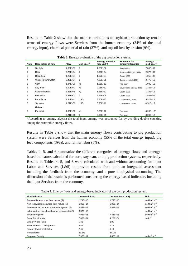
23
Results in Table 2 show that the main contributions to soybean production system in
terms of emergy flows were Services from the human economy (34% of the total
emergy input), chemical potential of rain (27%), and topsoil loss by erosion (9%).
Table 3. Emergy evaluation of the pig production system.
Note Description of flow Flow Unit kgpig-1
Emergy intensity (seJ unit-1)
Reference for Emergy intensities
Emergy (seJ kgpig
-1)
1 Sunlight 7.06E+07 J 1.00E+00 By definition 7.06E+07
2 Rain 6.75E+04 J 3.06E+04 Brown and Ulgiati, 2004b 2.07E+09
3 Deep heat 1.22E+04 J 1.02E+04 Odum, 1996 1.25E+08
4 Water (groundwater) 6.47E+04 J 4.28E+05 Bastianoni et al., 2001 2.77E+10
5 Corn 1.84E+00 kg 1.05E+12 This study 1.93E+12
5 Soy meal 3.90E-01 kg 2.98E+12 Cavalett and Ortega, 2009 1.16E+12
5 Other minerals 6.88E-02 kg 1.68E+12 Odum, 1996 1.16E+11
6 Electricity 5.53E+03 J 2.77E+05 Odum, 1996 1.53E+09
7 Local labor 1.44E-01 USD 3.70E+12 Coelho et al., 1999 5.31E+11
8 Services 1.22E+00 USD 3.70E+12 Coelho et al., 1999 4.51E+12
Output
9 Pig meat 1.00E+00 kg 8.28E+12 This study 8.28E+12*
9.21E+06 J 8.99E+05 This study 8.28E+12
*According to emergy algebra the total input emergy was accounted for by avoiding double counting
among the renewable emergy flows.
Results in Table 3 show that the main emergy flows contributing to pig production
system were Services from the human economy (55% of the total emergy input), pig
feed components (39%), and farmer labor (6%).
Tables 4, 5, and 6 summarize the different categories of emergy flows and emergy-
based indicators calculated for corn, soybean, and pig production systems, respectively.
Results in Tables 4, 5, and 6 were calculated with and without accounting for input
Labor and Services (L&S) to provide results from both an integrated assessment
including the feedback from the economy, and a pure biophysical accounting. The
discussion of the results is performed considering the emergy-based indicators including
the input Services from the economy.
Table 4. Emergy flows and emergy-based indicators of the corn production system.
Flow/Indicator Corn (with L&S) Corn (without L&S) Unit
Renewable resources from nature (R) 1.79E+15 1.79E+15 seJ ha-1 yr-1
Non-renewable resources from nature (N) 5.05E+14 5.05E+14 seJ ha-1 yr-1
Purchased inputs from outside the system (F) 2.55E+15 2.55E+15 seJ ha-1 yr-1
Labor and services from human economy (L&S) 3.07E+15 --- seJ ha-1 yr-1
Total emergy (U) 7.92E+15 4.85E+15 seJ ha-1 yr-1
Solar Transformity 7.00E+04 4.28E+04 seJ J-1
Emergy Yield Ratio 1.41 1.90
Environmental Loading Ratio 3.42 1.71
Emergy Investment Ratio 2.45 1.11
Renewability 22.6% 37.0%
Empower Density 7.92E+11 4.85E+11 seJ m-2 yr-1

24
Table 5. Emergy flows and emergy-based indicators of the soybean production system.
Flow/Indicator Soybean (with Labor & Services)
Soybean (without L&S) Unit
Renewable resources from nature (R) 1.79E+15 1.79E+15 seJ ha-1 yr-1
Non-renewable resources from nature (N) 5.72E+14 5.72E+14 seJ ha-1 yr-1
Purchased inputs from outside the system (F) 1.64E+15 1.64E+15 seJ ha-1 yr-1
Labor and services from human economy (L&S) 2.18E+15 --- seJ ha-1 yr-1
Total emergy (U) 6.19E+15 4.01E+15 seJ ha-1 yr-1
Solar Transformity 1.04E+05 6.72E+04 seJ J-1
Emergy Yield Ratio 1.62 2.44
Environmental Loading Ratio 2.45 1.24
Emergy Investment Ratio 1.62 0.70
Renewability 29.0% 44.7%
Empower Density 6.19E+11 4.01E+11 seJ m-2 yr-1
Table 6. Emergy flows and emergy-based indicators of the pig production system.
Flow/Indicator Pig meat (with Labor & Services)
Pig meat (without L&S) Unit
Renewable resources from nature (R) 2.19E+09 2.19E+09 seJ kgpig-1
Non-renewable resources from nature (N) 2.77E+10 2.77E+10 seJ kgpig-1
Purchased inputs from outside the system (F) 3.21E+12 3.21E+12 seJ kgpig-1
Labor and services from human economy (L&S) 5.05E+12 --- seJ kgpig-1
Total emergy (U) 8.28E+12 3.24E+12 seJ kgpig-1
Solar Transformity 8.99E+05 3.51E+05 seJ J-1
Emergy Yield Ratio 1.00 1.01
Environmental Loading Ratio 3780 1476
Emergy Investment Ratio 276 107
Renewability 0.03% 0.07%
Empower Density 6.77E+14 2.65E+14 seJ m-2 yr-1
The Solar Transformity (total emergy invested into the process divided by the energy
content of the product) calculated for pig meat (8.99∙105 seJ J
-1) was much higher than
for corn (7.00∙104 seJ J
-1) and soybean (1.04∙10
5 seJ J
-1), indicating that the pig
production system requires a higher global environmental support to produce one Joule
of product. These results confirmed how pig production occupies a higher position
within the energy hierarchy of the whole production chain due to its feature as an
animal production system.
The Emergy Yield Ratio (EYR = U/F) is a measure of the ability of a process to exploit
and make available local resources by investing outside resources. It provides a measure
of the appropriation of local resources by a process, which can be read as a potential
additional contribution to the economy, generated by investing resources already
available. The higher this value the more able is the process to exploit and make
available resources from nature per unit of investment from economy. The EYR for
corn and soybean were 1.41 (Table 4) and 1.62 (Table 5), while the pig production
showed an EYR of 1.00 (Table 6). The lowest possible value of the EYR is one, which
indicates that the emergy converging to generate the yield does not differ significantly

25
from the emergy invested from outside the system to drive the process. The latter is not
usefully exploiting any local resource. Therefore, processes with EYR equal to one or
only slightly higher do not provide significant net emergy to the economy and only
transform resources that are already available from previous processes. In so doing they
act as consumer processes more than creating new opportunities for the system’s
growth.
The Environmental Loading Ratio (ELR = (N+F) / R) is designed to compare the
amount of non-renewable and purchased emergy flows (N+F) to the amount of locally
renewable emergy (R). In the absence of investments from outside, the renewable
emergy that is locally available would have driven the growth of a mature ecosystem
consistent with the constraints imposed by the environment and characterized by an
ELR=0. Instead, the non-renewable imported emergy drives a different site
development, whose distance from the natural ecosystem can be indicated by the ELR.
The higher this ratio, the bigger the distance of the development from the natural
process that could have developed locally without non-renewable investment from
outside. In a way, the ELR is a measure of the disturbance to the local environmental
dynamics, generated by the development driven from outside sources. The ELR for pig
production system indicates that the non-renewable fraction of the total emergy is 3,780
times higher than the renewable part (Table 6), while the same indicator for corn and
soybean was 3.42 and 2.45 (Tables 4 and 5).
The Renewability indicator shows that the pig production system was supported by a
very small contribution of renewable resources (0.03%). For this reason it could be
considered like an industrial activity that is supported almost exclusively by human-
driven economic resources coming from outside the system. The intensification of pig
production over the last decades using smaller areas and industrial feed stuffs has been
based on the massive use of fossil energy in all steps of the production chain. This is
also reflected by the very high ELR and unitary value of the EYR calculated for the pig
production system (Table 6). In contrast, the soybean production subsystem showed a
renewability of 29.0% (Table 5), meaning that 71% of the inputs supporting the process
were related to non-renewable sources of emergy. The same indicator calculated for
corn production system was even lower: 22.6% (Table 4).
The Emergy Investment Ratio (EIR = F / (R+N)) indicates the proportion of purchased
resources from the economy in relation to the free resources from nature used by the
production system. The EIR value calculated for pig production system (276) was
much higher than the value calculated for corn (2.45) and soybean (1.62) production
systems (Tables 4, 5, and 6). For example, this figure shows that the pig production
system uses 276 times more resources purchased from the economy than free resources
26
from environment. The soybean production showed itself to be the system that uses the
lowest proportion of purchased resources between all evaluated systems.
The Empower Density (ED = U/area per time) measures the amount of emergy invested
per unit of area over time. ED may suggest land as a limiting factor for a process or, in
other words, may suggest the need for a given amount of support land around the
system, for it to be sustainable. The ED of the pig production system (6.77∙1014
seJ m-2
year-1
) was much higher than the ED of the soybean (6.19∙1011
seJ m-2
year-1
), and corn
(7.92∙1011
seJ m-2
year-1
) production systems (Tables 4, 5, and 6), proving how the pig
production subsystem is much more intensive in the use of resources per unit of area
than the investigated agricultural crops.
3.2 Embodied Energy Analysis
The embodied energy demand was evaluated by first quantifying the raw data input
flows to the production systems, and then multiplying the input flows by their specific
oil equivalent factors (obtained from literature after an accurate evaluation of their
conformity to the investigated process). Then, the embodied energy demand for each
input flow was added to account for the total energy demand of the process. The ratio
between the total energy demand and generated product made possible the calculation
of the energy intensity factor for each product (energy demand per kg of product). This
indicator quantifies the contribution of the investigated process to fossil energy
resources depletion. Tables 7, 8, and 9 show the Embodied Energy Analysis for corn,
soybean and pig production systems, respectively.
Table 7 shows that about 0.05 kg of crude oil equivalent was necessary to produce 1 kg
of corn. The total energy demand of the inputs was 1.36∙1010
J ha-1
year-1
(Table 7). The
total energy content of the corn output was 1.13∙1011
J ha-1
year-1
. These figures translate
into an Energy Return on Investment (EROI) of 8.3 (about 8 joules of corn were
produced per joule of fossil fuel invested in the production process). The main
contributions to the corn production system in terms of embodied energy were nitrogen
fertilizer (44% of the total energy demand), fuel (18%) and limestone (16%) (Table 7).
Table 8 shows that about 0.05 kg of crude oil equivalent was used to produce 1 kg of
soybean. The total energy demand of the inputs was 5.83∙109
J ha-1
year-1
(Table 8). The
total energy content of the soybean output was 5.96∙1010
J ha-1
year-1
. These figures
translate into an EROI of 10.2 (about 10 joules of soybean were produced per joule of
fossil fuel invested in the production process). The main contributions to the soybean
production system were fuel (37%), limestone (22%) and phosphorous fertilizer (14%)
(Table 8).

27
Table 7. Embodied energy analysis of the corn production system.
Note Description of flow Flow Units
Oil equivalent (kg oil unit-1)
Reference for oil equivalent
Total oil demand (kg oil equiv.)
Total energy demand (J)
1 Sunlight 5.77E+13 J * * * *
2 Rain 1.12E+07 kg * * * *
3 Deep heat 1.00E+10 J * * * *
4 Loss of topsoil 1.50E+04 kg * * * *
5 Limestone 3.50E+02 kg 0.15 Boustead and Hancock, 1979 5.27E+01 2.21E+09
6 Agrochemicals 1.02E+01 kg 1.43 Estimated from Ulgiati, 2001 1.45E+01 6.08E+08
7 Seeds 1.79E+01 kg 0.05 This study 8.93E-01 3.74E+07
8 Organic fertilizer 1.03E+03 kg * * * *
9 Nitrogen fertilizer 8.16E+01 kg 1.75 Estimated from Ulgiati, 2001 1.43E+02 5.98E+09
10 Phosphorus fertilizer 6.40E+01 kg 0.32 Estimated from Ulgiati, 2001 2.05E+01 8.58E+08
11 Potassium fertilizer 1.27E+02 kg 0.22 Estimated from Ulgiati, 2001 2.80E+01 1.17E+09
12 Fuel 4.81E+01 kg 1.23 Estimated from Ulgiati, 2001 5.92E+01 2.48E+09
13 Machinery (steel) 2.85E+00 kg 1.91 Estimated from Ulgiati, 2001 5.44E+00 2.28E+08
14 Local labor 4.78E+00 h * * * *
15 Services 8.21E+02 USD * * * *
Output
16 Corn 6.90E+03 kg 0.05 This study 3.24E+02 1.36E+10 (*) No oil equivalent factor was associated with this item within the scale of investigation.
Table 8. Embodied energy analysis of the soybean production system.
Note Description of flow Flow Units
Oil equivalent (kg oil unit-1)
Reference for oil equivalent
Total oil demand (kg oil equiv.)
Total energy demand (J)
1 Sunlight 5.77E+13 J * * * *
2 Rain 1.12E+07 kg * * * *
3 Deep heat 1.00E+10 J * * * *
4 Loss of topsoil 1.70E+04 kg * * * *
5 Limestone 2.00E+02 kg 0.15 Boustead and Hancock, 1979 3.01E+01 1.26E+09
6 Agrochemicals 1.05E+01 kg 1.43 Estimated from Ulgiati, 2001 1.50E+01 6.27E+08
7 Seeds 6.50E+01 kg 0.09 This study 5.85E+00 2.45E+08
8 Organic fertilizer 1.03E+03 kg * * * *
9 Nitrogen fertilizer 0.00E+00 kg 1.75 Estimated from Ulgiati, 2001 0.00E+00 0.00E+00
10 Phosphorus fertilizer 6.00E+01 kg 0.32 Estimated from Ulgiati, 2001 1.92E+01 8.04E+08
11 Potassium fertilizer 6.00E+01 kg 0.22 Estimated from Ulgiati, 2001 1.32E+01 5.53E+08
12 Fuel 4.16E+01 kg 1.23 Estimated from Ulgiati, 2001 5.12E+01 2.14E+09
13 Machinery (steel) 2.50E+00 kg 1.91 Estimated from Ulgiati, 2001 4.78E+00 2.00E+08
14 Local labor 4.62E+00 h * * * *
15 Services 5.80E+02 USD * * * *
Output
16 Soybean 3.00E+03 kg 0.05 This study 1.39E+02 5.83E+09 (*) No oil equivalent factor was associated with this item within the scale of investigation.
Table 9 shows that about 0.22 kg of crude oil equivalent was used to produce 1 kg of
live pig meat. The total energy demand of the inputs was 9.13∙106
J kgpig-1
(Table 9).
The total energy content of the pig meat output was 9.21∙106
J kgpig-1
. These figures
translate into an EROI of approximately 1.0 (i.e., one joule of pig meat was produced
per joule of fossil fuel invested in the production process).

28
Table 9. Embodied energy analysis of the pig production system.
Note Description of flow Flow Units
Oil equivalent (kg oil unit-1)
Reference for oil equivalent
Total oil demand (kg oil equiv.)
Total energy demand (J)
1 Sunlight 7.06E+07 J * * * *
2 Rain 6.75E+04 J * * * *
3 Deep heat 1.22E+04 J * * * *
4 Water (groundwater) 1.31E+01 kg 1.43E-04 Boustead and Hancock,1979 1.87E-03 7.84E+04
5 Corn 1.84E+00 kg 0.05 This study 8.63E-02 3.61E+06
5 Soy meal 3.90E-01 kg 0.08 Cavalett and Ortega, 2009 3.12E-02 1.31E+06
5 Other minerals 6.88E-02 kg 1.43 Estimated from Ulgiati, 2001 9.85E-02 4.12E+06
6 Electricity 5.53E+03 J 6.97E-08 Biondi et al., 1989 3.85E-04 1.61E+04
7 Local labor 7.22E-02 h * * * *
8 Services 1.22E+00 USD * * * *
Output
9 Pig meat 1.00E+00 kg 0.22 This study 2.18E-01 9.13E+06 (*) No oil equivalent factor was associated with this item within the scale of investigation.
As expected, the most important contributions for pig production system in terms of
embodied energy were the components of pig feed (99% of total inputs). These results
are in accordance with those obtained by Angonese et al. (2006) for pig production
system in Southern Brazil.
3.3 Material Flow Accounting
Local mass flows to the production systems were quantified and multiplied by
appropriate material intensity factors (obtained from literature after an accurate
evaluation of their conformity to the investigated process) to calculate the total material
demand on a larger scale and the relative material intensities of the products. In so
doing, the environmental disturbance generated by the withdrawal of resources over the
production systems was assessed. Tables 10, 11, and 12 show the material flow
accounting for corn, soybean, and pig production systems, respectively.
Results in Table 10 show that 1.82 kg of abiotic material, 1.77 kg of water, 0.02 kg of
air (used in chemical reactions), and 0.09 kg of biotic materials were used to produce 1
kg of corn. The total material flow demand resulted in 3.7 kg per kg of corn. The main
inputs to the abiotic impact factor in corn production system were topsoil loss by
erosion (77% of the total inputs), potassium fertilizer (11%) and limestone (5%). The
main inputs to the water impact factor were topsoil loss by erosion (36% of the total
inputs), limestone (28%) and phosphorous fertilizer (12%). The main inputs to the air
impact factor were phosphorous fertilizer (70%), limestone (18%) and potassium
fertilizer (8%). The main inputs to the biotic impact factor were topsoil loss by erosion
(91% of the total inputs) and organic fertilizer (8%). It is important to remark that
scientific literature usually provides poor data on the biotic impact factor as this impact
factor is not considered in most studies.

29
Results in Table 11 show that 4.25 kg of abiotic material, 3.49 kg of water, 0.03 kg of
air, and 0.24 kg of biotic materials were used to produce 1 kg of soybean. The total
material flow demand resulted in 8 kg per kg of soybean produced. The main inputs to
the abiotic impact factor in the soybean production system were topsoil loss by erosion
(88% of the total inputs), potassium fertilizer (5%), and limestone (3%). The main
inputs to the water impact factor were topsoil loss by erosion (49% of the total inputs),
limestone (19%), and phosphorous fertilizer (13%). The main inputs to the air impact
factor were phosphorous fertilizer (80%), limestone (12%), and potassium fertilizer
(4%). The main inputs to the biotic impact factor were topsoil loss by erosion (93% of
the total inputs) and organic fertilizer (7%).
Results in Table 12 show that 4.99 kg of abiotic material, 22.36 kg of water, 0.08 kg of
air, and 0.17 kg of biotic materials were needed to produce 1 kg of pig meat. The total
material flow demand resulted in 27.6 kg per kg of pig meat produced. The main inputs
to the abiotic impact factor in pig meat production system were corn (67% of the total
inputs) and soy meal (29%) used as feed stuffs, and direct water use (3%). The main
inputs to the water impact factor were direct water use (76 % of the total inputs), corn
(15%) and soy meal used as feed (9%). The main inputs to the air impact factor were
soy meal (41%) and corn (40%) used as feed, and direct water use (17%). The main
input to the biotic impact factor was the corn used as feeding stuffs.
The material flow demand was much higher in the pig production than in the corn and
soybean production systems. This is because the pig production system is a more
intensive production process relying on external material resources. Agrochemicals use
and topsoil loss are other important material indicators in agricultural production
systems. Soybean production uses about 3.49 g of agrochemicals and 5.7 kg of topsoil
per kilogram of soybean produced. Corn production uses about 1.47 g of agrochemicals
and 2.2 kg of topsoil per kilogram of corn produced (Tables 10 and 11).

30
Table 10. Material flow accounting of the corn production system.
Note Description of flow Flow Units
MIF abiotic (kg unit-1)
Mass Abiotic (kg)
MIF water (kg unit-1)
Mass Water (kg)
MIF air (kg unit-1)
Mass Air (kg)
MIF biotic (kg unit-1)
Mass Biotic (kg) Ref. for MIF
1 Sunlight 5.77E+13 J * * * * * * * *
2 Rain 1.12E+07 kg * * * * * * * *
3 Deep heat 1.00E+10 J * * * * * * * *
4 Loss of topsoil 1.50E+04 kg 0.66 9.90E+03 0.30 4.50E+03 0.00 0.00E+00 0.04 6.00E+02 By definition
5 Limestone 3.50E+02 kg 1.66 5.81E+02 9.70 3.40E+03 0.06 2.10E+01 0.00 0.00E+00 Wurbs et al., 1996
6 Agrochemicals 1.02E+01 kg 1.10 1.12E+01 0.00 0.00E+00 0.00 0.00E+00 0.00 0.00E+00 Our calculations based on literature data
7 Seeds 1.79E+01 kg 4.71 8.41E+01 4.94 8.82E+01 0.05 8.93E-01 0.24 4.28E+00 This study
8 Organic fertilizer 1.03E+03 kg 0.20 2.07E+02 0.75 7.75E+02 0.00 0.00E+00 0.05 5.17E+01 Our calculations based on literature data
9 Nitrogen fertilizer 8.16E+01 kg 1.10 8.98E+01 0.00 0.00E+00 0.00 0.00E+00 0.00 0.00E+00 Our calculations based on literature data
10 Phosphorus fertilizer 6.40E+01 kg 3.44 2.20E+02 23.30 1.49E+03 1.29 8.26E+01 0.00 0.00E+00 Wurbs et al., 1996
11 Potassium fertilizer 1.27E+02 kg 11.32 1.44E+03 10.60 1.35E+03 0.07 8.90E+00 0.00 0.00E+00 Wurbs et al., 1996 12 Fuel 4.81E+01 kg 1.36 6.54E+01 9.70 4.66E+02 0.02 9.14E-01 0.00 0.00E+00 Wurbs et al., 1996 13 Machinery (steel) 2.85E+00 kg 9.32 2.65E+01 81.90 2.33E+02 0.77 2.20E+00 0.00 0.00E+00 Wurbs et al., 1996 14 Local labor 4.78E+00 h * * * * * * * *
15 Services 8.21E+02 USD * * * * * * * *
Output
16 Corn 6.90E+03 kg 1.82 1.25E+04 1.77 1.22E+04 0.02 1.16E+02 0.09 6.52E+02 This study
(*) No material intensity factor (MIF) was associated to this item within the scale of investigation.

31
Table 11. Material flow accounting of the soybean production system.
Note Description of flow Flow Units
MIF abiotic (kg unit-1)
Mass Abiotic (kg)
MIF water (kg unit-1)
Mass Water (kg)
MIF air (kg unit-1)
Mass Air (kg)
MIF biotic (kg unit-1)
Mass Biotic (kg) Ref. for MIF
1 Sunlight 5.77E+13 J * * * * * * * *
2 Rain 1.80E+07 kg * * * * * * * *
3 Deep heat 1.00E+10 J * * * * * * * *
4 Loss of topsoil 1.70E+04 kg 0.66 1.12E+04 0.30 5.10E+03 0.00 0.00E+00 0.04 6.80E+02 By definition
5 Limestone 2.00E+02 kg 1.66 3.32E+02 9.70 1.94E+03 0.06 1.20E+01 0.00 0.00E+00 Wurbs et al., 1996
6 Agrochemicals 1.05E+01 kg 1.10 1.15E+01 0.00 0.00E+00 0.00 0.00E+00 0.00 0.00E+00 Our calculations based on literature data
7 Seeds 6.50E+01 kg 4.71 3.06E+02 4.94 3.21E+02 0.05 3.25E+00 0.24 1.56E+01 This study
8 Organic fertilizer 1.03E+03 kg 0.20 2.07E+02 0.75 7.75E+02 0.00 0.00E+00 0.05 5.17E+01 Estimative
9 Nitrogen fertilizer 0.00E+00 kg 1.10 0.00E+00 0.00 0.00E+00 0.00 0.00E+00 0.00 0.00E+00 Our calculations based on literature data
10 Phosphorus fertilizer 6.00E+01 kg 3.44 2.06E+02 23.30 1.40E+03 1.29 7.74E+01 0.00 0.00E+00 Wurbs et al., 1996
11 Potassium fertilizer 6.00E+01 kg 11.32 6.79E+02 10.60 6.36E+02 0.07 4.20E+00 0.00 0.00E+00 Wurbs et al., 1996 12 Fuel 4.16E+01 kg 1.36 5.66E+01 9.70 4.03E+02 0.02 7.90E-01 0.00 0.00E+00 Wurbs et al., 1996 13 Machinery (steel) 2.50E+00 kg 9.32 2.33E+01 81.90 2.05E+02 0.77 1.93E+00 0.00 0.00E+00 Wurbs et al., 1996 14 Local labor 4.62E+00 h * * * * * * * *
15 Services 5.80E+02 USD * * * * * * * *
Output
16 Soybean 3.00E+03 kg 4.25 1.27E+04 3.49 1.05E+04 0.03 9.63E+01 0.24 7.32E+02 This study
(*) No material intensity factor (MIF) was associated to this item within the scale of investigation.

32
Table 12. Material flow accounting of the pig production system.
Note Description of flow Flow Units
MIF abiotic (kg unit-1)
Mass Abiotic (kg)
MIF water (kg unit-1)
Mass Water (kg)
MIF air (kg unit-1)
Mass Air (kg)
MIF biotic (kg unit-1)
Mass Biotic (kg) Ref. for MIF
1 Sunlight 7.06E+07 J * * * * * * * *
2 Rain 6.75E+04 J * * * * * * * *
3 Deep heat 1.22E+04 J * * * * * * * *
4 Water (groundwater) 1.31E+01 kg 0.01 1.31E-01 1.30 1.70E+01 0.00 1.31E-02 0.00 0.00E+00 Wurbs et al., 1996
5 Corn 1.84E+00 kg 1.82 3.34E+00 1.77 3.25E+00 0.02 3.07E-02 0.09 1.73E-01 This study
5 Soy meal 3.90E-01 kg 3.67 1.43E+00 4.94 1.93E+00 0.08 3.12E-02 0.00 0.00E+00 Cavalett and Ortega, 2009
5 Other minerals 6.88E-02 kg 1.24 8.53E-02 2.30 1.58E-01 0.02 1.38E-03 0.00 0.00E+00 Wurbs et al., 1996
6 Electricity 1.54E-03 kWh 2.09 3.21E-03 5.86 9.00E-03 0.37 5.68E-04 0.00 0.00E+00 Hinterberger and Stiller, 1998. Modified.
7 Local labor 7.22E-02 h * * * * * * * *
8 Services 1.22E+00 USD * * * * * * * *
Output
9 Pig meat 1 kg 4.99 4.99E+00 22.36 2.24E+01 0.08 7.70E-02 0.17 1.73E-01 This study
(*) No material intensity factor (MIF) was associated to this item within the scale of investigation.

33
3.4 Life Cycle Assessment
The Life Cycle Inventory developed in this study was based on the calculation
procedures reported in Annex 1, 2, and 3. The items considered in this study were:
Emissions from manufacturing and application of fertilizers, limestone,
herbicides, pesticides, fungicides, and insecticides in agricultural systems.
Emissions from manufacturing of diesel used in agricultural operations.
Emissions from manufacturing of machinery (tractors, implements, harvesters)
used in agricultural operations.
Emissions from manufacturing of the pig feed components (simplified as corn,
soy meal, and chemicals in general), electricity, and water used in the pig
production system.
Local emissions of N2O from nitrogen fertilizers and N2O and CO2 from urea.
Local emissions of CO2 from limestone.
Local emissions of CO2 from diesel in motor vehicles used in agricultural
operations.
Local emissions of NH3 and N2O from manure management and CH4 from
enteric fermentation and manure management in the pig production system.
Local emissions of nitrogen, phosphorous, and potassium from manure spread in
agricultural soils were not accounted for due to lack of data on these emissions
and also to avoid double accounting with the manure emissions in the pig
production systems.
The results from the life cycle inventory made possible the assessment of different
environmental impact categories by means of the CML 2 Baseline 2000 v2.05 method.
This calculation step was performed using the software package SimaPro® (PRé
Consultants B.V.). Tables 13, 14 and 15 show the environmental impact indicators
calculated for corn, soybean, and pig production systems. The functional unit
considered in this LCA is one kg of output.
In Figure 5, the relative contribution of different inputs to the corn production system is
depicted. Fertilizers were responsible for the vast majority of the environmental impacts
in all the categories except in global warming potential (GWP) and ozone depletion
potential (ODP). In terms of GWP, the local emissions (i.e., N2O and CO2 from nitrogen
fertilizer and limestone use, and CO2 from diesel used in the agricultural operations)
played a crucial role. However, in terms of ODP, the use of agrochemicals (insecticides,
fungicides, herbicides and pesticides) was the main source of impact.
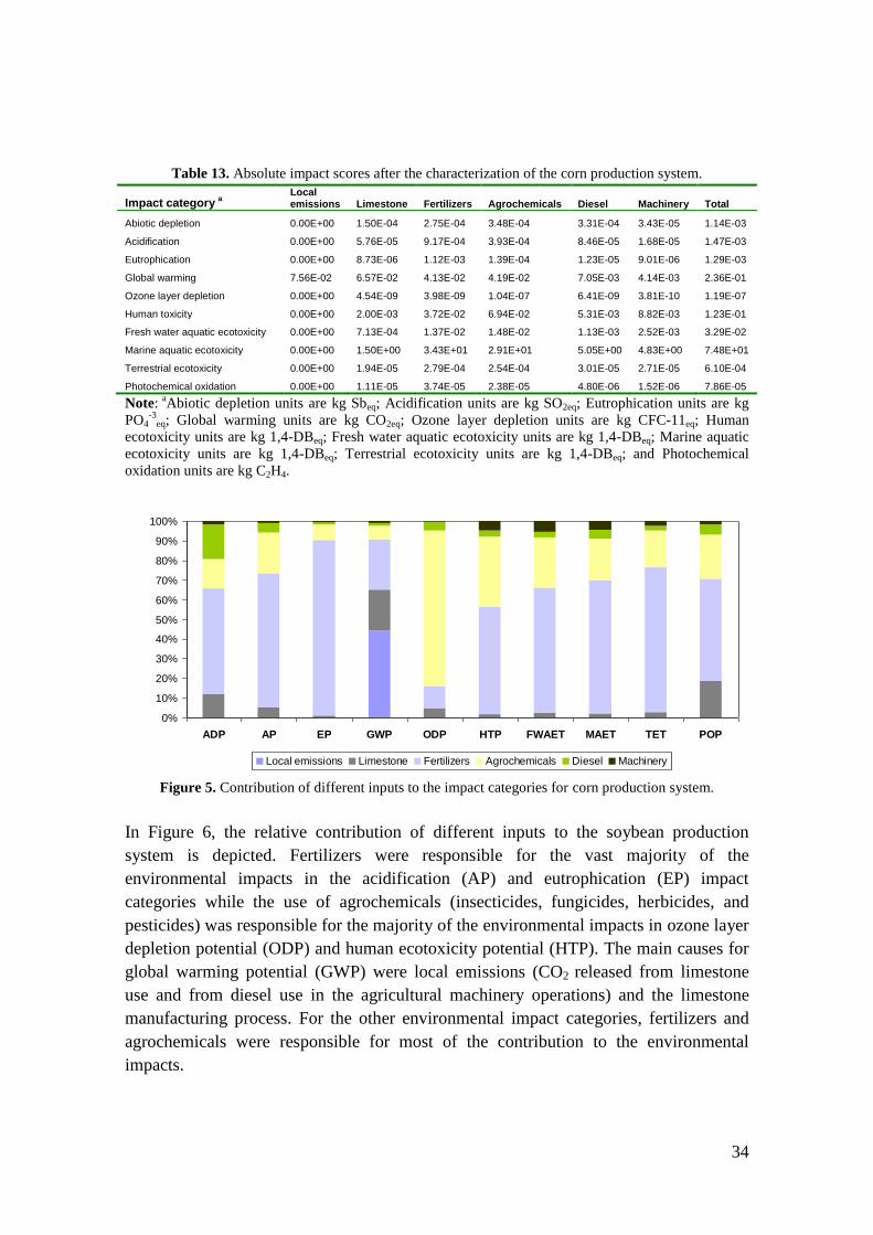
34
Table 13. Absolute impact scores after the characterization of the corn production system.
Impact category a Local emissions Limestone Fertilizers Agrochemicals Diesel Machinery Total
Abiotic depletion 0.00E+00 1.50E-04 2.75E-04 3.48E-04 3.31E-04 3.43E-05 1.14E-03
Acidification 0.00E+00 5.76E-05 9.17E-04 3.93E-04 8.46E-05 1.68E-05 1.47E-03
Eutrophication 0.00E+00 8.73E-06 1.12E-03 1.39E-04 1.23E-05 9.01E-06 1.29E-03
Global warming 7.56E-02 6.57E-02 4.13E-02 4.19E-02 7.05E-03 4.14E-03 2.36E-01
Ozone layer depletion 0.00E+00 4.54E-09 3.98E-09 1.04E-07 6.41E-09 3.81E-10 1.19E-07
Human toxicity 0.00E+00 2.00E-03 3.72E-02 6.94E-02 5.31E-03 8.82E-03 1.23E-01
Fresh water aquatic ecotoxicity 0.00E+00 7.13E-04 1.37E-02 1.48E-02 1.13E-03 2.52E-03 3.29E-02
Marine aquatic ecotoxicity 0.00E+00 1.50E+00 3.43E+01 2.91E+01 5.05E+00 4.83E+00 7.48E+01
Terrestrial ecotoxicity 0.00E+00 1.94E-05 2.79E-04 2.54E-04 3.01E-05 2.71E-05 6.10E-04
Photochemical oxidation 0.00E+00 1.11E-05 3.74E-05 2.38E-05 4.80E-06 1.52E-06 7.86E-05
Note: a
Abiotic depletion units are kg Sbeq; Acidification units are kg SO2eq; Eutrophication units are kg
PO4-3
eq; Global warming units are kg CO2eq; Ozone layer depletion units are kg CFC-11eq; Human
ecotoxicity units are kg 1,4-DBeq; Fresh water aquatic ecotoxicity units are kg 1,4-DBeq; Marine aquatic
ecotoxicity units are kg 1,4-DBeq; Terrestrial ecotoxicity units are kg 1,4-DBeq; and Photochemical
oxidation units are kg C2H4.
0%
10%
20%
30%
40%
50%
60%
70%
80%
90%
100%
ADP AP EP GWP ODP HTP FWAET MAET TET POP
Local emissions Limestone Fertilizers Agrochemicals Diesel Machinery
Figure 5. Contribution of different inputs to the impact categories for corn production system.
In Figure 6, the relative contribution of different inputs to the soybean production
system is depicted. Fertilizers were responsible for the vast majority of the
environmental impacts in the acidification (AP) and eutrophication (EP) impact
categories while the use of agrochemicals (insecticides, fungicides, herbicides, and
pesticides) was responsible for the majority of the environmental impacts in ozone layer
depletion potential (ODP) and human ecotoxicity potential (HTP). The main causes for
global warming potential (GWP) were local emissions (CO2 released from limestone
use and from diesel use in the agricultural machinery operations) and the limestone
manufacturing process. For the other environmental impact categories, fertilizers and
agrochemicals were responsible for most of the contribution to the environmental
impacts.

35
Table 14. Absolute impact scores after the characterization of the soybean production system.
Impact category a Local emissions Limestone Fertilizers Agrochemicals Diesel Machinery Total
Abiotic depletion 0.00E+00 1.14E-04 5.09E-04 1.39E-04 1.67E-04 1.71E-05 9.45E-04
Acidification 0.00E+00 4.38E-05 5.76E-04 1.74E-04 4.25E-05 8.31E-06 8.44E-04
Eutrophication 0.00E+00 6.65E-06 5.68E-04 5.14E-05 6.16E-06 4.43E-06 6.37E-04
Global warming 1.05E-01 5.00E-02 6.08E-02 1.67E-02 3.54E-03 2.06E-03 2.38E-01
Ozone layer depletion 0.00E+00 3.45E-09 7.52E-09 5.47E-08 3.22E-09 1.91E-10 6.91E-08
Human toxicity 0.00E+00 1.52E-03 4.72E-02 3.07E-02 2.67E-03 4.33E-03 8.64E-02
Fresh water aquatic ecotoxicity 0.00E+00 5.43E-04 1.42E-02 5.76E-03 5.70E-04 1.24E-03 2.23E-02
Marine aquatic ecotoxicity 0.00E+00 1.14E+00 3.69E+01 1.15E+01 2.54E+00 2.37E+00 5.45E+01
Terrestrial ecotoxicity 0.00E+00 1.48E-05 4.19E-04 1.06E-04 1.51E-05 1.33E-05 5.68E-04
Photochemical oxidation 0.00E+00 8.44E-06 2.35E-05 1.01E-05 2.41E-06 7.51E-07 4.53E-05
Note: a
Abiotic depletion units are kg Sbeq; Acidification units are kg SO2eq; Eutrophication units are kg
PO4-3
eq; Global warming units are kg CO2eq; Ozone layer depletion units are kg CFC-11eq; Human
ecotoxicity units are kg 1,4-DBeq; Fresh water aquatic ecotoxicity units are kg 1,4-DBeq; Marine aquatic
ecotoxicity units are kg 1,4-DBeq; Terrestrial ecotoxicity units are kg 1,4-DBeq; and Photochemical
oxidation units are kg C2H4.
0%
10%
20%
30%
40%
50%
60%
70%
80%
90%
100%
ADP AP EP GWP ODP HTP FWAET MAET TET POP
Local emissions Limestone Fertilizers Agrochemicals Diesel Machinery
Figure 6. Contribution of different inputs to the impact categories for soybean production system.
In Figure 7, the relative contribution of different inputs to the pig production system is
depicted. Pig feed ingredients were responsible for the highest environmental impacts in
most of the categories. However, local emissions (NH3, N2O, and CH4 from manure
management and enteric fermentation of pigs) caused the highest contribution in the
acidification (AP) and global warming potential (GWP) impact categories. The corn
used as pig feed was responsible for most of the impacts in the categories of abiotic
depletion (ADP), ozone depletion potential (ODP), and marine, freshwater, and
terrestrial ecotoxicities (MAET, FWAET, and TET). In the photochemical oxidation
(POP) impact category, soy meal showed the highest contribution. In the eutrophication

36
(EP) impact category, local emissions and soy meal represented the highest
contribution.
Table 15. Absolute impact scores after characterization for pig production system.
Impact category a Local emissions
Feed - Corn
Feed - Soy meal
Feed - Minerals Electricity Water Total
Abiotic depletion 0.00E+00 1.74E-03 5.50E-04 8.32E-05 8.91E-07 2.75E-05 2.40E-03
Acidification 8.96E-03 1.55E-03 1.45E-03 6.07E-05 3.11E-07 1.82E-05 1.20E-02
Eutrophication 1.96E-03 1.17E-03 1.92E-03 4.60E-05 8.86E-08 1.14E-05 5.11E-03
Global warming 1.01E+00 4.39E-01 5.28E-01 1.24E-02 3.31E-04 4.15E-03 2.00E+00
Ozone layer depletion 0.00E+00 1.27E-07 1.03E-08 7.45E-10 1.25E-11 1.95E-10 1.38E-07
Human toxicity 5.60E-04 1.59E-01 1.65E-01 2.26E-02 5.22E-05 2.32E-03 3.49E-01
Fresh water aquatic ecotoxicity 0.00E+00 4.10E-02 1.10E-02 9.19E-03 1.43E-05 2.27E-03 6.35E-02
Marine aquatic ecotoxicity 0.00E+00 1.00E+02 2.25E+01 1.93E+01 2.96E-02 4.32E+00 1.46E+02
Terrestrial ecotoxicity 0.00E+00 1.04E-03 9.41E-05 8.42E-05 6.08E-07 2.41E-05 1.25E-03
Photochemical oxidation 1.95E-04 8.33E-05 1.59E-03 2.81E-06 7.27E-08 1.27E-06 1.88E-03
Note: a
Abiotic depletion units are kg Sbeq; Acidification units are kg SO2eq; Eutrophication units are kg
PO4-3
eq; Global warming units are kg CO2eq; Ozone layer depletion units are kg CFC-11eq; Human
ecotoxicity units are kg 1,4-DBeq; Fresh water aquatic ecotoxicity units are kg 1,4-DBeq; Marine aquatic
ecotoxicity units are kg 1,4-DBeq; Terrestrial ecotoxicity units are kg 1,4-DBeq; and Photochemical
oxidation units are kg C2H4.
Although water use showed a low contribution to the environmental impact indicators
in the LCA, water resource use figured remarkably high in the pig production system as
showed in the inventory data and by both the material flow accounting and water
footprint results (Chapters 3.3 and 3.6). These results reinforce the necessity of a multi-
criteria assessment framework to calculate a set of complementary indicators able to
fully explore different aspects of process performance and sustainability.
0%
20%
40%
60%
80%
100%
ADP AP EP GWP ODP HTP FWAET MAET TET POP
Local emissions Feed - Corn Feed - Soy meal Feed - Minerals Electricity Water
Figure 7. Contribution of different inputs to the impact categories for pig production system.
Figure 8 shows the comparative environmental impacts for corn, soybean and pig
production systems. The environmental impact scores showed higher results for pig
production in all the environmental impact categories compared to corn and soybean

37
production. Corn production presented lower environmental impacts in comparison to
soybean in all the categories except in the global warming potential (GWP). Results
showed that high toxicity indicators were obtained in corn and soybean production
systems due to the massive use of agrochemicals in these crop production systems.
The results obtained from this study pointed out that efforts in improving pig meat
production should be mostly related to improvements in feed production due to its
preponderance among the production inputs. The same conclusions were reached by
Cederberg and Flysjö (2004). Proper feed production and consumption may lead to a
lower amount of nutrients in manure per unit product. Low content of nitrogen in
manure is a possible measure to reduce emissions of ammonia, methane, and nitrous
oxide from the whole production chain. Crop rotation and low agrichemical use in the
production of grains used as pig feed stuffs are other possible measures to reduce
environmental impacts. Locally produced feeding stuffs reduce the environmental
impacts from transport and increase the possibilities of beneficial integration of crop
and swine production. New advanced techniques could be used for proper manure
treatment and utilization in Brazil (Kunz et al., 2009). Such techniques (for instance,
enhancement of solid-liquid separation using flocculants) are compatible with the new
reality of Brazilian industrial swine production, which has emerged as a major
competitor in the international market (Kunz et al., 2009).
0%
10%
20%
30%
40%
50%
60%
70%
80%
90%
100%
ADP AP EP GWP ODP HTP FWAET MAET TET POP
Corn Soybean Swine
Figure 8. Comparison of environmental impact categories for corn,
soybean, and swine production systems.
Careful planning for manure application in agricultural soils can also significantly
reduce emissions from reactive nitrogen and provide savings in the use of chemical
fertilizers, thus reducing the use of purchased non-renewable energy sources coming
from outside the production area. An integrated farming system with proper balance

38
between animals and fodder crops presents good opportunities to minimize nutrient loss
and resource use while maintaining self-sufficiency of the production system.
3.5 Ecological Footprint
The calculation of the Ecological Footprint (EF) was based on the direct (or indirect in
the case of pig feed ingredients in the pig production system) area required for growing
soybean or corn crops and the forest area required to sequester CO2 equivalent emitted
by all inputs used in the production system. Tables 16, 17 and 18 show the ecological
footprint calculations for corn, soybean, and pig production systems.
The total Ecological Footprint of corn production was 3.69∙10-4
gha/kg (Table 16). The
direct agricultural area used in corn production accounted for 87% of the EF while the
area necessary to absorb the carbon dioxide equivalent related to the inputs used in the
corn production process was responsible for 13% of the EF.
Table 16. Ecological Footprint of the corn production system.
Description Value Unit Reference
Cultivated area 1.45E-04 ha/kg This study
Crop Yield Factor 2.21 gha/ha Kitzes, 2009
Crop EF 3.20E-04 gha/kg
Area to absorb theCO2 equivalent related to the inputs use
CO2 equivalent inputs 1644 kg/ha This study (LCA results)
Output (kg) 6.90E+03 kg/ha/ This study
Forest area CO2 potential fixation 6600 kg CO2/ha/yr Wackernagel and Rees, 1996
Area to absorb the CO2 equivalent 3.61E-05 ha/yr
Forest Yield Factor 1.34 gha/ha Kitzes, 2009
Forest EF 4.84E-05 gha/kg
Total Ecological Footprint of corn 3.69E-04 gha/kg
Table 17. Ecological Footprint of the soybean production system.
Description Value Unit Reference
Cultivated area 3.33E-04 ha/kg This study
Crop Yield Factor 2.21 gha/ha Kitzes, 2009
Crop EF 7.37E-04 gha/kg
Area to absorb the CO2 equivalent related to the inputs use
CO2 equivalent inputs 707 kg/ha This study (LCA results)
Output (kg) 3.00E+03 kg/ha This study
Forest area CO2 potential fixation 6600 kg CO2/ha/yr Wackernagel and Rees, 1996
Area to absorb the CO2 equivalent 3.57E-05 ha/yr
Forest Yield Factor 1.34 gha/ha Kitzes, 2009
Forest EF 4.78E-05 gha/kg
Total Ecological Footprint of soybean 7.85E-04 gha/kg

39
The total Ecological Footprint of soybean production was 7.85∙10-4
gha/kg (Table 17).
The direct agricultural area used in soybean production was responsible for 94% of the
EF while the area necessary to absorb the carbon dioxide equivalent related to the
production inputs was responsible for 6% of the EF.
Concerning pig production, the total Ecological Footprint was 1.35∙10-3
gha/kg (Table
18). Results show that the indirect agricultural area cropped to produce corn and soy
meal-based feeding stuffs was responsible for 43% and 27% of the EF. The area
necessary to absorb the carbon dioxide equivalent related to the inputs used in the pig
production process was responsible for 30% of the EF.
Table 18. Ecological Footprint of the pig production system.
Description Value Unit Reference
Cultivated area corn 2.66E-04 ha/kg This study
Crop Yield Factor 2.21 gha/ha Kitzes, 2009
Corn crop EF 5.88E-04 gha/kg
Cultivated area soy meal 1.62E-04 ha/kg
Crop Yield Factor 2.21 gha/ha Kitzes, 2009
Soy meal crop EF 3.59E-04 gha/kg
Area to absorb the CO2 equivalent related to the inputs use
CO2 equivalent inputs 1.997 kg/kg This study (LCA results)
Output (kg) 1.00E+00 kg This study
Forest area CO2 potential fixation 6600 kg CO2/ha/yr Wackernagel and Rees, 1996
Area to absorb the CO2 equivalent 3.03E-04 ha/yr
Forest Yield Factor 1.34 gha/ha Kitzes, 2009
Forest EF 4.06E-04 gha/kg
Total Ecological Footprint of pig 1.35E-03 gha/kg
Figure 9 shows the comparison of the Ecological Footprints calculated for corn,
soybean and pig production systems. The results pointed out that the EF of pig
production (1.35∙10-3
gha kg-1
) is higher than the EF of corn (3.69∙10-4
gha kg-1
) and
soybean (7.85∙10-4
gha kg-1
) productions, confirming the high intensity of pig
production process.
0
0,0001
0,0002
0,0003
0,0004
0,0005
0,0006
0,0007
0,0008
0,0009
0,001
Corn Soybean Pig
Eco
log
ica
l fo
otp
rin
t (g
ha
/kg
) Crop
CO2 Fixation
Figure 9. Comparison of the Ecological Footprint indicator of corn, soybean, and pig production systems.

40
3.6 Water Footprint
The calculation of the Water Footprint (WF) was based on three components: 1) green
water footprint (consumptive use of rainwater); 2) blue water footprint (consumptive
use of surface or groundwater); and 3) grey water footprint (volume of polluted water
associated to the production of goods and services). The sum of these three components
generates the total Water Footprint.
The green component for corn and soybean crops were obtained by adding the green
water evapotranspiration over the growing period to water incorporated into the product
(water content of the product). In the case of pig production, the green component was
derived from the indirect green water footprints related to the main pig feed stuffs (corn
and soy meal).
There was no blue water footprint in the corn and soybean production because no
surface or groundwater was used for crop irrigation in the Toledo River basin. For the
pig production system, the blue water footprint was calculated by taking into account
drinking and service water used during pig production lifetime (Annex 3).
The grey component was calculated as the load of pollutants that enters the water
system divided by the difference between the ambient water quality standard for that
pollutant (the maximum acceptable concentration) and its natural concentration in the
receiving water body. In the soybean and corn production systems the nitrogen
emissions were related to the nitrogen from synthetic fertilizers and organic fertilizers
(pig manure). In the pig production system the nitrogen emissions were related to the
nitrogen from manure. The quantity of nitrogen that reaches free flowing water bodies
was assumed to be 10% of the applied fertilization rate (Hoekstra et al., 2009). The total
volume of water required per kg of nitrogen was calculated considering the volume of
nitrogen leached and its maximum allowable concentration in free flowing surface
water bodies. Due to the absence of local ambient water quality standards for nitrogen,
we used the standard recommended by the US EPA for nitrate in water: 10 mg/liter
(measured as N) (EPA, 2005). This limit was used to calculate the volume of freshwater
required to assimilate the load of pollutants. Due to lack of available data on natural
concentrations in receiving water bodies, the natural concentration was assumed to be
zero. Tables 19, 20 and 21 show the water footprint calculated for corn, soybean and pig
production systems.
The total Water Footprint of corn production was 937 liters per kilogram of corn (Table
19). Results in Table 19 show that the green water footprint (810 l kg-1
) was responsible
for 86% of the total water footprint indicator while the grey water footprint (127 l kg-1
)

41
was responsible for 14% of the total water footprint. There was no blue water footprint
because no surface or groundwater was used for crop irrigation of corn in the Toledo
River basin. The calculated green water footprint value for corn resulted much higher
than that showed by Aldaya and Llamas (2008) for corn in Spain (around 400 m3 per
hectare). However, in the corn production system in Spain about 6000 m3 per hectare of
blue water resources were needed to complement green water use. By considering both
green and blue water footprint the results obtained in this study are comparable to those
obtained by Aldaya and Llamas (2008) for corn in Spain (927 l kg-1
).
The Water Footprints calculated for corn (Table 19) were also comparable to those
calculated by Mekonnen and Hoekstra (2010) for corn production at global average.
Mekonnen and Hoekstra (2010) obtained the following figures for corn production:
green water footprint 947 l kg-1
; blue water footprint 81 l kg-1
; grey water footprint 194 l
kg-1
. Total water footprint for corn production at global average was then 1,222 l kg-1
which is comparable to the value calculated for corn in the present study (937 l kg-1
).
This is also because corn production systems in the Toledo River basin do not require
the blue water component in the production process.
Table 19. Water Footprint for corn production system.
Description Value Unit Ref.
Green WF
Evaporation 8.10E+02 l/kg See Annex 1
Incorporation 2.00E-01 l/kg
Total WF green 8.10E+02 l/kg
Blue WF
Evaporation 0.00E+00 l/kg
Incorporation 0.00E+00 l/kg
Lost return 0.00E+00 l/kg
Total WF blue 0.00E+00 l/kg
Grey WF
Nitrogen from fertilizers 8.16E+01 kg/ha/yr See Annex 1
Nitrogen from organic fertilizer (manure) 5.82E+00 kg/ha/yr See Annex 1
Total nitrogen leacheda 8.74E+00 kg/ha/yr
Nitrogen limit on environmentb 1.00E+01 mg/l EPA, 2005
Total WF grey 1.27E+02 l/kg
Total WF 9.37E+02 l/kg a Nitrogen leaching to the water bodies estimated as 10% of total nitrogen used. b By absence of local ambient water quality standards for nitrogen, the standard recommended by the US EPA for nitrate in water was used: 10 mg/liter (measured as N).
The total Water Footprint of soybean production was 1,880 liters per kilogram of
soybean (Table 20). Results in Table 20 show that the green water footprint indicator
(1,860 l kg-1
) was responsible for 99% of the total water footprint indicator while the
grey water footprint (19.4 l kg-1
) was responsible for only 1% of the total water
footprint. Also for soybean, there was no blue water footprint because no surface or
groundwater was used for crop irrigation. The grey water footprint of the soybean

42
production was lower than that of the corn because the soybean plant is able to
assimilate nitrogen from atmosphere and no complement of nitrogen is necessary as
synthetic fertilizers in this production system. Apparently, in the case of soybean
production nitrogen is not the most critical pollutant. Due to the lack of available data
on limits of phosphorous, potassium or agrochemicals residue emissions in local water
bodies, it was not possible to perform a more accurate calculation of the grey water
footprint component for soybean production.
Mekonnen and Hoekstra (2010) presented the following figures for soybean production
at global average: green water footprint 2,037 l kg-1
, blue water footprint 70 l kg-1
, and
grey water footprint 37 l kg-1
. Total water footprint for soybean production at global
average was then 2,145 l kg-1
. These figures are comparable with the value calculated
for soybean production system in the present study (Table 20).
Table 20. Water Footprint for soybean production system.
Description Value Unit Ref.
Green WF
Evaporation 1.86E+03 l/kg See Annex 2
Incorporation 1.20E-01 l/kg
Total WF green 1.86E+03 l/kg
Blue WF
Evaporation 0.00E+00 l/kg
Incorporation 0.00E+00 l/kg
Lost return 0.00E+00 l/kg
Total WF blue 0.00E+00 l/kg
Grey WF
Nitrogen from fertilizers 0.00E+00 kg/ha/yr See Annex 2
Nitrogen from organic fertilizer (manure) 5.82E+00 kg/ha/yr See Annex 2
Total nitrogen leacheda 5.82E-01 kg/ha/yr
Nitrogen limit on environmentb 1.00E+01 mg/l EPA, 2005
Total WF grey 1.94E+01 l/kg
Total WF 1.88E+03 l/kg a Nitrogen leaching to the water bodies estimated as 10% of total nitrogen used. b in the absence of local ambient water quality standards for nitrogen, we have used the standard recommended by the US EPA for nitrate in water: 10 mg/liter (measured as N).
The total Water Footprint of pig production was 2,740 liters per kilogram of pig meat
(Table 21). Results in Table 21 show that the green water footprint (2,390 l kg-1
) from
the indirect inputs (corn and soy meal) used as pig feeding stuffs was responsible for
87% of the total water footprint while the blue footprint indicator (13.1 l kg-1
) was
responsible for only 1% of the total water footprint. The blue water footprint refers to
the direct groundwater used in the pig production while the grey water footprint refers
to the water necessary for diluting the nitrogen leaching from the pig manure. The grey
water footprint (332 l kg-1
) was responsible for 12% of the total water footprint. In this
study it was assumed that only 10% of total nitrogen content in manure is emitted to the
water bodies. If all the manure was released to the water bodies the grey water footprint

43
would increase up to 3,318 l kgpig-1
(an increase of 109% in the total water footprint
indicator for this production system). Release of pig manure in water bodies is
forbidden by Brazilian environmental legislation although this practice still occurs. In
Figure 10 the water footprint components calculated for corn, soybean, and pig
production are compared.
Table 21. Water Footprint for pig production system.
Description Value Unit Ref.
Green WF
Indirect from corn production 1.49E+03 l/kgpig See Annex 1
Indirect from soy meal production 9.08E+02 l/kgpig See Annex 2
Total WF green 2.39E+03 l/kgpig
Blue WF
Evaporation 0.00E+00 l/kgpig
Incorporation 0.00E+00 l/kgpig
Lost return 1.31E+01 l/kgpig See Annex 3
Total WF blue 1.31E+01 l/kgpig
Grey WF
Nitrogen leached from manurea 3.32E-03 kg/kgpig See Annex 3
Nitrogen limit on environmentb 1.00E+01 mg/l EPA, 2005
Total WF grey 3.32E+02 l/kgpig
Total WF 2.74E+03 l/kgpig a Nitrogen leaching to the water bodies estimated as 10% of total present in manure produced. b In the absence of local ambient water quality standards for nitrogen, we have used the standard recommended by the US EPA for nitrate in water: 10 mg/liter (measured as N).
0
500
1000
1500
2000
2500
3000
Corn Soybean Pig
Wa
ter
foo
tpri
nt (
l/kg
)
Green Water Footprint
Blue Water Footprint
Grey Water Footprint
Figure 10. Comparison of the Water Footprint for corn, soybean, and pig production systems.
The indicators of water use calculated by applying the Water Footprint method were
much higher than the water intensity factors calculated by means of the Material Flow
Accounting (Tables 10, 11, and 12). This is because the Material Flow Accounting
method evaluates direct and indirect water use corresponding only to the Blue Water
Footprint component of a production process. Conventionally, statistics on water use
focus on measuring water withdrawals and direct water use. Hoekstra et al. (2009)
pointed out that the Water Footprint accounting method is characterized by a much

44
broader perspective. First of all, Water Footprint measures both direct and indirect water
use, where the latter refers to water use in the supply chain of a product. The Water
Footprint thus links final consumers and intermediate businesses and traders to the
water use along the whole production chain of a product. This is relevant because
generally the direct water use of a consumer is small compared to its indirect water use,
and the operational water use of a business is generally small if compared to the supply-
chain water use. Consequently, the picture of the actual water requirement for a product
can change radically. The Water Footprint method looks at water consumption (not only
to withdrawal) also referring to the part of the water withdrawal that gets lost through
evaporation (i.e., the part of the water withdrawal that does not return to the system
from which it has been withdrawn). Summarizing, Water Footprint looks not only at
blue water use (i.e., use of surface and ground water) but it also includes a green water
footprint component (use of rainwater) and a grey water footprint component (polluted
water).
Data used in the calculations of the present study were obtained from the closest
meteorological station to the Toledo River basin. Since the green water footprint
component is very important in the investigated production systems, it would be
important to improve the quality of data on specific evapotranspiration measurements
for the evaluated crops in the Toledo River basin. Site specific data on
evapotranspiration in the Toledo River basin as well as standardized evapotranspiration
measurements could improve water footprint calculations.
3.7 Carbon Footprint
The Carbon Footprint was assessed by using data from the LCA (GWP category). Table
22 and Figure 11 show the comparative results of Carbon Footprint for corn, soybean
and pig production systems divided into primary (local emissions) and secondary
(related to the inputs to the production process) Carbon Footprints.
Table 22. Comparison of the Carbon Footprints for corn, soybean and pig production systems.
Component Corn Soybean Pig Unit
Primary Carbon Footprint 0.11 0.08 1.01 kg CO2eq/kg
Secondary Carbon Footprint 0.13 0.16 0.98 kg CO2eq/kg
Total Carbon Footprint 0.24 0.24 2.00 kg CO2eq/kg

45
0,00
0,20
0,40
0,60
0,80
1,00
1,20
Corn Soybean Pig
kgC
O2
eq
/kg
Primary Carbon Footprint
Secondary Carbon Footprint
Figure 11. Comparison of the Carbon Footprints for corn, soybean and pig production systems.
Results in Table 22 show that corn and soybean production systems are characterized by
the same Carbon Footprint: 0.24 kg of CO2 equivalent is released per kg of generated
products. Although the investigated corn production system shows higher primary
Carbon Footprint than soybean, the soybean production system shows higher secondary
Carbon Footprint than the corn system. This means that the corn production system has
higher local emissions (probably due to higher emissions from nitrogen in chemical
fertilizers) while the soybean production system uses more inputs in the production
process. Finally, the pig production system showed the highest Carbon Footprint: about
2 kg of CO2 equivalent released per kilogram of pig meat produced.
3.8 Performance and sustainability indicators: scenario analysis
The purpose of this section is to explore the environmental performance and
sustainability of the investigated production systems at basin level through alternative
scenarios based on multi-criteria assessment methods and indicators (Table 23).
The Toledo River basin has a total area of about 9,292 ha and a population of
approximately 550 inhabitants. The land use is divided as follows: agricultural area
6,460 ha (69.5%); pasture 160 ha (1.7%); water 29 ha (0.3%); original forest 1,116 ha
(12.0%); urban area 1,528 ha (16.4%). In the agricultural area of this basin 11,000 pigs
per year are also farmed. In the scenario analysis the soybean-corn intercrop was
assumed to occupy the entire agricultural area of the Toledo River basin since it is the
main crop activity in the basin.
Indicators calculated at farm level were upscaled at basin level to assess the
environmental impacts at regional scale focusing on three main scenarios:

46
Base Scenario: this scenario is based on the current land uses listed above and
on the inputs supporting corn, soybean and pig production systems in the Toledo
River basin as detailed in Annexes 1, 2, and 3.
Scenario A: this scenario considers a decrease of 50% in pig production in the
Toledo basin and substitution of the agricultural area by original forest until the
basin area reaches 20% of forest area, as it is requested by the Brazilian forest
law. Scenario A is also based on the following assumptions: (a) the use of more
appropriate soil management techniques reduces soil loss by 50% compared to
the Base Scenario; (b) appropriate measures for water savings reduce water use
in pig production by 50%; (c) appropriate manure management techniques
reduce local emissions of N2O, NH3, and CH4 from manure by 50%; (d)
biological pest control reduces agrochemicals use in corn and soybean
production systems by 50%.
Scenario B: this scenario considers an increase of 50% in pig production in the
Toledo River basin and the spreading of the agricultural area over the remaining
original forest until the latter decreases to only 5% of the total basin area.
Scenario B is also based on the following assumptions: (a) without using
appropriate soil management techniques soil loss increases by 50% compared to
the Base Scenario; (b) due to lack of proper water management, water use in pig
production system increases by 50%; (c) inappropriate manure management
techniques increase local emissions of N2O, NH3, and CH4 from pig manure by
50%; (d) more resistant agricultural pests will increase the use of agrochemicals
by 50% in both corn and soybean production systems.
Table 23 shows selected environmental indicators calculated to draw and evaluate the
three alternative scenarios for the Toledo River basin. In line with the best option
suggested by Scenario A, all indicators decrease in Scenario A compared to the Base
Scenario and Scenario B. This highlights the crucial role played by the assumption
made in Scenario A in terms of the environmental performance and sustainability of the
investigated production systems.
A comparison among a large set of multi-criteria indicators calculated for three
alternative scenarios (Base Scenario, Scenarios A, and B) is shown through a radar
diagram in Figure 12. To enable the comparison among indicators with different orders
of magnitude, a normalization procedure was applied. Indicators were normalized from
Table 23 by dividing all the values of Scenarios A and B by the corresponding value of
the Base Scenario.

47
Table 23. Environmental indicators selected to draw three alternative scenarios for the Toledo River
basin.
Indicator Base Scenario Scenario A Scenario B Units per year
Energy input 1.36E+14 1.13E+14 1.59E+14 Joule
Abiotic resources 1.69E+08 8.70E+07 2.64E+08 kg
Water resources 1.73E+08 1.10E+08 2.51E+08 kg
Air resources 1.46E+06 1.25E+06 1.66E+06 kg
Biotic resources 9.15E+06 4.35E+06 1.47E+07 kg
Emergy input 1.01E+20 8.11E+19 1.21E+20 seJ
Ecological footprint 3.33E+04 2.86E+04 3.77E+04 global ha
Green water footprint 7.51E+10 6.53E+10 8.39E+10 Liter
Blue water footprint 1.58E+07 3.96E+06 3.56E+07 Liter
Grey water footprint 6.42E+09 5.19E+09 7.65E+09 Liter
Agrochemicals use 1.33E+08 5.89E+07 2.20E+08 g
Soil loss 2.07E+08 9.14E+07 3.42E+08 kg
Abiotic depletion 6.71E+04 5.25E+04 8.22E+04 kg Sb eq
Acidification 8.07E+04 5.62E+04 1.11E+05 kg SO2 eq
Eutrophication 5.95E+04 4.75E+04 7.26E+04 kg PO4 eq
Global warming (Carbon Footprint) 1.76E+07 1.36E+07 2.21E+07 kg CO2 eq
Ozone layer depletion (ODP) 5.56E+00 2.88E+00 8.64E+00 kg CFC-11 eq
Human toxicity 6.65E+06 4.52E+06 8.99E+06 kg 1.4-DB eq
Fresh water aquatic ecotoxicity 1.71E+06 1.24E+06 2.21E+06 kg 1.4-DB eq
Marine aquatic ecotoxicity 4.05E+09 3.04E+09 5.13E+09 kg 1.4-DB eq
Terrestrial ecotoxicity 3.86E+04 2.93E+04 4.85E+04 kg 1.4-DB eq
Photochemical oxidation 5.81E+03 3.80E+03 7.99E+03 kg C2H4
Figure 12. Comparison among three alternative scenarios: Base Scenario, Scenario A, and Scenario B.

48
Considering that a wider area means a higher environmental impact, Scenario A shows
a smaller impact compared to Scenario B and Base Scenario. Such an outcome can be
explained by considering that the assumptions made in Scenario A involve not only a
lower direct consumption of inputs but also lower indirect emissions as well as indirect
consumption of energy, material and environmental support.
Results of different scenarios may differ depending on goal, boundaries, time scale and
different management schemes, thus suggesting different optimization procedures.
Ulgiati et al. (2003) pointed out that assessing a process performance on different scales
offers significant ways to refine the analysis and improve the process.
Agrochemicals use and soil loss are important mass flow indicators for agricultural
production systems. The figure of 133 tons of agrochemicals used every year in the
Toledo River basin (Base Scenario) proves the intensity of agrochemical use in the
basin, indicating its high contribution to environmental problems and water pollution in
the region. The Toledo River basin plays an important role in water and sediment
contribution to the reservoir of the Itaipu Binacional dam. The topsoil loss due to
agricultural activities in the basin is about 207,000 tons per year. This amount of topsoil
loss becomes sediment into the dam decreasing its life span. This highlights the
interaction between agricultural production systems in the Toledo River basin and other
important economic sectors in Brazil (e.g., electricity generation). Therefore, proper soil
management techniques are urgently needed not only to preserve the ability of
agroecosystems to provide goods and services but also to avoid potential negative
feedback on other productive sectors.
The total emergy is a measure of environmental support (work done by nature)
provided to productive systems. In principle, the higher the imported non-renewable
emergy use, the less sustainable is the system. In this regard, the emergy theory
suggests that high-transformity products should be properly used to reinforce (amplify)
the process by feeding back high-quality emergy to the lower (low-transformity) levels
of the system. An appropriate use of environmental support increases sustainability.
The demand for environmental support, here measured by the emergy intensity
indicator, appears to be a fundamental performance category, suggesting patterns for
appropriate use of products. In the Base Scenario, the emergy-based indicators show
that soybean, corn and pig production systems require an environmental support of
1.01∙1020
seJ year-1
. If this emergy flow could be provided only by renewable
resources, an area equivalent to 56,364 ha would be necessary. This value is about 6.1
times higher than the total area of the basin considering all land uses.

49
The Ecological Footprint indicator shows that the area required to produce the inputs
used in the production process and to assimilate the wastes produced by the three
production systems is equivalent to 33,300 hectares. This area is about 3.6 times higher
than the total area of the basin. Ecological Footprint is a measure of the “ecological
deficit” showing the dependence of the Toledo basin on ecosystem services generated
outside its political boundary. This is an important indication of unsustainability as there
is strong competition for using the limited area of productive land in the world.
An important environmental benefit of biomass production should be the carbon
neutrality between carbon absorption and emissions: the carbon emitted by utilizing
biomass should be balanced by the carbon absorbed in the photosynthetic growing of
biomass, thus having a carbon neutral balance. On investigating the entire production
chain, it most often emerges that this condition is not satisfied. The Life Cycle
Assessment showed that the Carbon Footprint (global warming potential) of the three
production systems (corn, soybean, and pig) upscaled to the basin level is equivalent to
the emissions of 17,600 tons of CO2 per year (Base Scenario). Through better
management practices assumed in Scenario A, it would be possible to reduce the
Carbon Footprint by 22% compared to the present situation (Base Scenario). However,
in the case of Scenario B the Carbon Footprint would increase by 26% compared to the
current situation. In the same way, in Scenario A, acidification and eutrophication
would decrease by 20% and 30% compared to the Base Scenario.
It is worth noting that, while the global warming potential (Carbon Footprint) is related
to global biosphere processes and climate change aspects, the acidification and
eutrophication potentials are mainly related to local regional-scale impacts generated
on the sites where the process occurs.
The indicator of water resource use calculated in the Material Flow Accounting shows
that the amount of water directly and indirectly used for soybean, corn, and pig
production systems in the Toledo River basin (Base Scenario) is equivalent to the water
supplying a city of 3,314 inhabitants (considering an average water use of 143 liters
person-1
day-1
in urban areas of Brazil). This figure is more than six times higher than
the population living in the Toledo River basin.
The Water Footprint indicators show that the total water required by the investigated
processes (green and blue water) and the water used for wastes dilution (grey water) at
the Toledo River basin level is equal to 82 million m3 per year (Base Scenario).
Considering an average water use of 143 liters person-1
day-1
, the amount of water
directly and indirectly used for soybean, corn, and pig production systems at the Toledo
basin level is equivalent to the water supply for a city of 1.5 million inhabitants. This

50
figure highlights the huge impact of the three production systems on local water
resources. Results in Table 23 show how the water footprint (green, blue, grey) is a
crucial factor when upscaling the production processes at basin level. In addition, the
high value of the green water footprint also points out the potentially high impact on
biodiversity due to reallocation of green evaporative flows from natural vegetation to
productive vegetation. Massive losses of original forest can heavily affect such a regime
shift. Grey water footprint is also an important component due to the high load of
agrochemicals on water bodies. Hoekstra et al. (2009) pointed out that grey water
footprint can be reduced to zero by preventing the application of chemicals to
agricultural fields. Grey water can be lowered substantially by applying less chemicals
and adopting better techniques and timing of application (so that less chemicals are
drained into water systems by leaching and runoff).
Agriculture is often focused on maximizing land productivity, which makes sense when
land is scarce and freshwater is very abundant. Instead, when water is the limiting
factor, maximizing water productivity becomes a crucial goal. This implies applying
less irrigation in a more efficient way and harvesting a higher yield per volume of water
evaporated. Because blue water originates from surface or groundwater, it has a larger
effect on the environment than green water use. The world’s blue water resources are
limited. Once we subtract from the total annual blue water flow the flows in remote
areas as well as flood flows and environmental flow requirements, we are left with a
limited volume of available blue water.
Local impacts may occur due to overexploitation or pollution of surface or groundwater
bodies or due to land use change. Environmental impacts at the river basin level may
occur when several exploitations and waste flows are added up causing downstream
impacts on aquatic and terrestrial ecosystems next to the river.
Mekonnen and Hoekstra (2010) presented a study that quantifies the green, blue and
grey water footprint of global crop production in a spatially-explicit way for the period
1996-2005. The study showed that corn production is responsible for 10% of the total
world water footprint while soybean production is responsible for 5% of the total world
water footprint.
In the Base Scenario, considering the land uses at basin level, agricultural crops are
responsible for 96% of the total Water Footprint in the Toledo River basin while pig
production system is responsible for only 4% of the total Water Footprint. This
proportion is very similar to the results obtained for the Guadiana River basin (Spain)
by Aldaya and Llamas (2008), where agricultural activities accounted for 95% of the
total Water Footprint.

51
Mekonnen and Hoekstra (2010) showed that the water footprint of crop production in
the Paraná River basin (the biggest hydrological basin that includes the Toledo River
basin) is as follows: green water footprint 237∙1012
l year-1
, blue water footprint 3.2∙1012
l year-1
, and grey water footprint 9.4∙1012
l year-1
. The total water footprint in the Paraná
River basin is 250∙1012
liters per year. If we divided the water footprint of the crops in
the Paraná River basin by its area (8.8∙107
ha) and the water footprint of the crops (corn
and soybean) in the Toledo River basin by its area (9.3∙103
ha), the comparative results
show that the green water footprint per unit of area calculated for Toledo River basin is
2.9 times higher than the green water footprint in the Parana River basin. In addition,
the grey water footprint per unit of area calculated in the Toledo River basin is 6.1 times
higher than in the Parana River basin. It was not possible to compare the blue water
footprint components because there is no blue water use in the Toledo River basin.
These figures highlight the higher intensity in water use per unit area in the Toledo
River basin since they are much higher than the average water footprint calculated for
agricultural activities in the whole region of Paraná River basin.
All these results prove the high intensity of materials, energy, emergy, and water use
due to agricultural and pig production activities in the Toledo River basin. The use of
these natural resources is exceeding the carrying capacity of the Toledo basin and is
sustained by eroding the stocks of natural resources at an unsustainable rate. Water
Footprint indicators in river basins can facilitate a more efficient allocation and use of
water resources, also providing a transparent interdisciplinary framework for policy
formulation.
It is important to notice that double counting may occur when evaluating green and grey
water footprint components at the basin level. The double counting in green water
footprint may occur when corn or soybean produced locally is used in pig production
systems. In this case, the indirect green water resources from corn and soy meal (from
soybean) produced locally should not be double counted. Double counting in grey water
may occur when pollution from pig manure is accounted for in pig production systems
and also in crop production systems when the manure is used as organic fertilizer in the
same crop production.
The application of an integrated multi-criteria assessment framework to alternative
scenarios generated performance and sustainability indicators calling for a twofold
optimization pattern: (a) to decrease the use of or replace those inputs affecting
material, energy, emergy, and water flows as well as the ecological and carbon
footprints; and (b) to decrease the use or avoid the misuse of the investigated products,
thus indirectly decrease the input demand by controlling the end of the life cycle chain.
Results on a local scale suggest that optimization strategies should be applied to the

52
investigated processes by means of a more efficient use of input flows as well as by
recycling wastes, by-products, and co-products, thus implementing so-called “zero-
emission production patterns”. Process clustering oriented to maximize matter and
energy flow exchanges (included wastes, by-products and co-products) within a
production pattern could be a viable strategy to improve the environmental performance
and sustainability in the long run. For example, a higher integration between
agricultural activities and pig farming systems could generate significant savings of
chemical fertilizers and feed stuffs at both farm and regional scales, reducing at the
same time the environmental impacts of these production activities.

53
4. Conclusion
The multi-criteria assessment framework developed in this study provided useful
information about the interactions and proper use of natural capital, human-driven
resources, and ecosystem services supporting the management of agricultural and
farming systems in the Toledo River basin (Brazil).
Quantifying the direct and indirect flows of water, matter, energy and money to and
from the investigated systems made possible a deeper understanding of their production
processes as well as a more detailed picture of their relationships with the surrounding
environment. Indicators of environmental performance highlighted the intensification
process occurring in the Toledo River basin over recent decades. The indicators of
environmental sustainability showed an increased dependence on non-renewable
resources, mainly imported from outside the system, supporting modern cropping and
pig production systems. The input flows showing a high impact on performance and
sustainability indicators were water and feeding stuffs used in the pig production and
agrochemicals, fertilizers and topsoil used in the soybean-corn production systems.
The analysis of three alternative scenarios explored the potential environmental impacts
associated with different options of natural resource management in the Toledo River
basin. The assumptions made in Scenario A showed a possible improvement of the
environmental performance and sustainability through a shift in land use and by
applying proper environmental management practices.
The multi-criteria assessment framework implemented in this study and the related set
of indicators provided a benchmark for future investigations as well as a useful support
to local managers and policy makers committed to developing environmental policies
based on sustainable management of agroecosystems. Better integration between
agricultural and farming activities in the Toledo River basin is worth further
investigation by means of both field and modeling studies. Crucial factors to investigate
are the intensive use of water, agrochemicals and the concentration of manure, all
related to the high intensity of agricultural and farming activities in the basin.
Acknowledgements
The authors wish to acknowledge the support of UNESCO-IHP in the framework of the
project “Water Programme for Environmental Sustainability” - contract n. 4500080116.
They are also grateful to Rafael González from the International Hydroinformatics
Center (PTI Itaipu) for providing data and assistance to set up the case study.

54
References
AGRIANUAL - Anuário da agricultura Brasileira, 2010. São Paulo, SP: FNP
Consultoria e Comércio. Editora Argos.
Aldaya M.M., Llamas M.R., 2008. Water footprint analysis for the Guadiana River
basin, Value of Water Research Report Series No. 35, UNESCO-IHE, Delft, the
Netherlands. Available at:
www.waterfootprint.org/Reports/Report35-WaterFootprint-Guadiana.pdf
Aldaya M.M., Hoekstra A.Y., 2009. The water needed to have Italians eat pasta and
pizza, Value of Water Research Report Series No. 36, UNESCO-IHE, Delft, the
Netherlands. Available at: http://www.waterfootprint.org/Reports/Report36-
WaterFootprint-Pasta-Pizza.pdf
Angonese A.R., Campos A.T., Zacarkim C.E., Matsuo M.S., Cunha F., 2006.
Eficiência energética de sistema de produção de suínos com tratamento dos
resíduos em biodigestor. Revista Brasileira de Engenharia Agrícola e Ambiental,
10(3), 745–750.
ANUALPEC - Anuário da agricultura Brasileira, 2010. São Paulo, SP: FNP Consultoria
e Comércio. Editora Argos.
Bargigli S., Raugei M., Ulgiati S., 2005. Mass flow analysis and mass-based indicators.
In: Jorgensen S.E., Costanza R., Xu F. (Eds.). Handbook of ecological indicators
for assessment of ecosystem health. CRC Press, 353–378.
Bastianoni S., Marchettini N., Panzieri M., Tiezzi E., 2001. Sustainability assessment of
a farm in the Chianti area (Italy). Journal of Cleaner Production 9, 365-373.
Biondi P., Panaro V., Pellizzi G., 1989. Le richieste di energia del sistema agricolo
italiano. CNR, Consiglio Nazionale delle Ricerche, Progetto Finalizzato
Energetica, Sottoprogetto Biomasse ed Agricoltura, Report LB-20, Roma, Italy,
389 pp.
Boustead I., Hancock G.F., 1979. Handbook of Industrial Energy Analysis. Ellis
Horwood Limited. England.
Brown M.T., Ulgiati S., 1999. Emergy evaluation of the biosphere and natural capital.
AMBIO 28, 486–493.
Brown M.T., Ulgiati S., 2004a. Energy quality, emergy, and transformity: H.T. Odum’s
contribution to quantifying and understanding systems. Ecological Modelling 178,
201-213.
Brown M.T., Ulgiati S., 2004b. Emergy analysis and environmental accounting. In:
Cleveland C, editor. Encyclopedia of energy. Oxford, UK: Academic Press,
Elsevier; p. 329-354.
Bulsink F., Hoekstra A.Y., Booij M.J., 2009. The water footprint of Indonesian
provinces related to the consumption of crop products, Value of Water Research

55
Report Series No. 37, UNESCO-IHE, Delft, the Netherlands. Available at:
www.waterfootprint.org/Reports/Report37-WaterFootprint-Indonesia.pdf
Buonocore E., Franzese P.P., Ulgiati S., 2012. Assessing the environmental
performance and sustainability of bioenergy production in Sweden: a life cycle
assessment perspective. Energy (Elsevier), 37, 69-78.
Castellini C., Bastianoni S., Granai C., Dal Bosco C. Brunetti M., 2006. Sustainability
of poultry production using the emergy approach: comparison of conventional and
organic rearing systems. Agriculture Ecosystems and Environment 114, 343–350.
Cavalett O., Queiroz J.F., Ortega E., 2006. Emergy assessment of integrated production
systems of grains, pig and fish in small farms in the South Brazil. Ecological
Modelling 296, 205-224.
Cavalett O., Ortega E., 2009. Emergy, nutrient balance, and economic assessment of
soybean production and industrialization in Brazil. Journal of Cleaner Production
17(8), 762-777.
Cavalett O., D’Angelo S., Franzese P.P., 2010. Energy and emergy evaluations of
agricultural and farming production systems in the Toledo River basin (Brazil). In:
Jesús Ramos-Martín, Mario Giampietro, Sergio Ulgiati, and Sandra G.F. Bukkens
(Editors). Can We Break the Addiction to Fossil Energy? Proceedings of the 7th
Biennial International Workshop Advances in Energy Studies, Barcelona, Spain,
19-21 October 2010, pp. 497-504 (ISBN 978-84-938852-9-8).
Cederberg C., Flysjö A., 2004. Environmental Assessment of future pig farming
systems - quantification of three scenarios from the FOOD 21 Synthesis work.
Report from the Swedish institute for food and biotechnology. SIK Rapport nr.
723 2004.
Coelho O., Ortega E., Comar V., 1999. Balanço de Emergia do Brasil (dados de 1996,
1985 e 1981). In: Ortega E, Safonov, Comar V. (Eds.), Introduction to Ecological
Engineering, with Brazilian case studies, Unicamp, Campinas, SP, Brazil.
CONAB, 2009. Área e produção das safras paranaense e brasileira 2007/08 e 2008/09.
Avaliable at:
http://www.conab.gov.br/conabweb/download/sureg/PR/Soja%20Junho%202009.
CONAMA (Conselho Nacional do Meio Ambiente), 2005. Resolução 357, Ministério
do Meio Ambiente, Brasil.
de Groot S.R., Mazur P., 1962. Non-equilibrium Thermodynamics. North-Holland,
Amsterdam.
EPA, 2005. List of drinking water contaminants: ground water and drinking water, US
Environmental Protection Agency. Available at:
www.epa.gov/safewater/mcl.html#1
European Council Regulation, 1999. Official Journal of the European Community v. 42,
n. 1804/1999.

56
FAO, 2005. Livestock Policy Brief. Responding the livestock revolution, Rome, p. 8.
FAO, 2006. Livestock‘s Long Shadow – Environmental Issues and Options, Rome, p.
377.
FAO, 2007. Key statistics of food and agriculture external trade. Food and Agricultural
Organization of the United Nations, Economic and Social Department, The
Statistics Division. Available at: http://faostat.fao.org/site/339/default.aspx
Franzese P.P., Dumontet S., Scopa A., Ulgiati S., 2005. Combined Use of Emergy
Synthesis and GIS for Environmental Sustainability Assessment: The Case of the
Roccamonfina Natural Park, Italy. In: Brown M.T., Campbell D., Comar V.,
Haung S.L., Rydberg T., Tilley D., Ulgiati S. (Eds.), Emergy Synthesis 3. Theory
and Applications of the Emergy Methodology. Center for Environmental Policy,
University of Florida, Gainesville, USA, pp. 311-327.
Franzese P.P., Russo G.F., Ulgiati S., 2008a. Modeling the interplay of environment,
economy and resources in marine protected areas. A case study in southern Italy.
Ecological Questions 10, 91-97.
Franzese P.P., Russo G.F., Ulgiati S., 2008b. GIS and Emergy Synthesis evaluation of
urban waste management. In: Barbir, F. and Ulgiati, S. (Eds.), Sustainable Energy
Production and Consumption. Benefits, Strategies and Environmental Costing.
Book of the NATO Series: Science for Peace and Security, 339-352. Springer.
Franzese P.P., Arico S., Viglia S., Russo G.F., Ulgiati S., 2009a. Emergy-based
evaluation of natural capital and ecosystem services: the case study of Astroni
wildlife reserve, Italy. In: Brown M.T., Campbell D., Comar V., Haung S.L.,
Rydberg T., Tilley D., Ulgiati S. (Eds.), EMERGY SYNTHESIS 5. Theory and
Applications of the Emergy Methodology. Center for Environmental Policy,
University of Florida, Gainesville, USA, pp. 55-64 (ISBN: 978-0-9707325-4-5).
Franzese P.P., Rydberg T., Russo G.F., Ulgiati S., 2009b. Sustainable biomass
production: a comparison between Gross Energy Requirement and Emergy
Synthesis methods. Ecological Indicators 9, 959-970.
Gelder J.W., Dros J.M., 2005. From rainforest to chicken breast: Effects of soybean
cultivation for animal feed on people and nature in the Amazon region – a chain of
custody study. Research report for the Dutch Soy Coalition commissioned by
Friends of the Earth Netherlands and Cordaid. Available at:
www.milieudefensie.nl/landbouw/publicaties/rapporten/From%20Rainforest%20t
o%20Chickenbreast.pdf
Gerbens-Leenes P.W., Hoekstra A.Y., van der Meer T.H., 2008a. Water footprint of
bio-energy and other primary energy carriers. Value of Water Research Report
Series No.29, UNESCO-IHE, Delft, The Netherlands. Available at:
http://www.waterfootprint.org/Reports/Report29-WaterFootprintBioenergy.pdf
Gerbens-Leenes P.W., Hoekstra A.Y., van der Meer T.H., 2008b. The water footprint of
bio-energy: global water use for bio-ethanol, bio-diesel, heat and electricity. Value
of Water Research Report Series No. 34, UNESCO-IHE, Delft, The Netherlands.
Available at:

57
https://files.pbworks.com/download/7mIriCrAp9/np-net/12639422/UNESCO-
IHE%20(2008)%20WaterFootprint-of-Bioenergy.pdf
Gomes M., Biondi A., Brianezi T., Glass V., 2008. O Brasil dos Agrocombustíveis:
Impactos das Lavouras sobre a Terra, o Meio e a Sociedade - Soja e Mamona
2008. Repórter Brasil. Available at:
http://www.reporterbrasil.com.br/agrocombustiveis/relatorio.php
Häyhä T., Franzese P.P., Ulgiati S., 2011. Economic and environmental performance of
electricity production in Finland: a multicriteria assessment framework.
Ecological Modelling, 223, 81-90.
Herendeen R., 1998. Embodied energy, embodied everything... now what? In: Ulgiati
S., Brown M.T., Giampietro M., Herendeen R.A. and Mayumi K. (Eds.), Book of
Proceedings of the International Workshop Advances in Energy Studies. Energy
Flows in the Ecology and Economy, Porto Venere, Italy, May 26/30, 1998, 13–48.
Hinterberger F., Stiller H., 1998. Energy and material flows. In: Ulgiati S., et al.,
editors. Advances in energy studies. Energy flows in ecology and economy.
Roma, Italy: Musis Publisher, 275–286.
Hirakuri M.H., 2008. Estimativa de Custo de Produção e Lucratividade da Soja, Safra
2008/09, para o Paraná e Santa Catarina. Circular Técnica 65, Embrapa. Available
at: http://www.cnpso.embrapa.br/download/cirtec/circtec65.pdf
Hoekstra A.Y., 2008. Water neutral: reducing and offsetting the impacts of water
footprints. Value of Water Research Report Series No.28, UNESCO-IHE, Delft,
The Netherlands. Available at:
www.waterfootprint.org/Reports/Report28-WaterNeutral.pdf
Hoekstra A.Y., Chapagain A.K., Aldaya M.M., Mekonnen M.M., 2009. Water Footprint
Manual. State of the Art 2009. Available at:
http://www.waterfootprint.org/downloads/WaterFootprintManual2009.pdf
IBGE (Instituto Brasileiro de Geografia e Estatística), 2006. Pesquisa Pecuária
Municipal. Available at: http://www.ibge.gov.br/
IBGE (Instituto Brasileiro de Geografia e Estatística), 2009. Produção Agrícola
Municipal 2008. Rio de Janeiro: IBGE.
IFIAS, 1974. Energy analysis. Workshop Report no. 6. Stockholm, 89 pp.
IPCC, 2006. Guidelines for national greenhouse gas inventories. Volume 4: Agriculture,
forestry and other land use. Available at:
http://www.ipcc-nggip.iges.or.jp/public/2006gl/vol4.html
ISO 14040, 2006. Environmental management - Life cycle assessment - Principles and
framework, The International Organization for Standardization.
ISO 14044, 2006. Environmental management - Life cycle assessment - Requirements
and guidelines, The International Organization for Standardization.
Kitzes J., 2009. Ecological footprint standards 2009 Version 3.2, Global Footprint
Network, Oakland, CA, USA. Available at: www.footprintstandards.org

58
Kunz A., Miele M., Steinmetz R.L.R., 2009. Advanced swine manure treatment and
utilization in Brazil. Bioresource Technology 100, 5485–5489.
Mekonnen M.M., Hoekstra A.Y., 2010. The green, blue and grey water footprint of
crops and derived crop products. Volume 1: Main Report. Value of Water
Research Report Series No.47, UNESCO-IHE, Delft, The Netherlands. Available
at: http://www.waterfootprint.org/?page=files/Publications
Miele M., Waquil P.D., 2007. Cadeia produtiva da carne suína. Revista de Política
Agrícola v. XVI, n. 1.
Nieweglowski A.M.A., 2006. Indicadores de qualidade da água na bacia hidrográfica do
rio Toledo – PR. Master thesis in Agronomy. State University of Paraná. 237pp.
Odum H.T., 1988. Self-organization, transformity, and information. Science 242, 1132–
1139.
Odum H.T., 1994. Ecological and General Systems. University Press of Colorado,
USA, 644 pp.
Odum H.T., 1996. Environmental accounting. Emergy and environmental decision
making. NY: John Wiley & Sons; ISBN 0-471-11442-1. p. 370.
Odum H.T., 2007. Environment, Power and Society for the Twenty-First Century: The
Hierarchy of Energy. Columbia University Press, USA, 432 pp.
Ortega E., Cavalett O., Bonifacio R., Watanabe M., 2005. Brazilian Soybean
Production: Emergy Analysis With an Expanded Scope. Bulletin of Science,
Technology & Society 25 (4), 323-334.
Pengue W.A., 2005. Transgenic Crops in Argentina: The Ecological and Social Debt.
Bulletin of Science, Technology & Society 25 (4), 314-322.
Pereira B.D., Maia J.C.S., Camilot R., 2008. Technical efficiency in swine breeding:
effect of the expenses with the environment and fiscal renunciation. Revista
Brasileira de Engenharia Agrícola e Ambiental 12 (2), 200–204.
Pinheiro Machado Filho L.C., da Silveira M.C.A.C., Hötzel M. J., Pinheiro Machado
L.C., 2001. Produção agroecológica de suínos – uma alternativa sustentável para a
pequena propriedade no Brasil. II Conferência Internacional Virtual sobre
Qualidade de Carne Suína. Available at:
http://www.freewebs.com/hotzel/Suino%20Organico%202001.pdf
PNMA II - Programa Nacional do Meio Ambiente II. 2002. Monitoramento da
Qualidade da água. Curitiba : Ministerio do Meio Ambiente, 64pp.
Prigogine I., 1947. Study of thermodynamics of Irreversible Processes, 3rd ed. Wiley,
New York.
Schmidt-Bleek F., 1993. MIPS re-visited. Fresenius Environmental Bulletin, 2, 407-12.
Seganfredo M.A., 1999. Os dejetos de suínos são um fertilizante ou um poluente do
solo? Cadernos de Ciência e Tecnologia 16, 129–141.

59
Seganfredo M.A., Girotto A.F., 2004. Custos de armazenagem e transporte de dejetos
de suínos usados como fertilizantes de solo. Embrapa Suínos e Aves, Comunicado
Técnico 474, 1–3.
Sharpley A., Meisinger J.J., Breeeuwsma A., Sims J.T., Daniel T.C., Schepers J.S.,
2002. Impacts of animal manure management on ground and surface water
quality. In: Hatfield J.L., Stewart B.A. (Eds.), Animal Waste Utilization: Effective
Use of Manure as a Soil Resource. Lewis Publishers, Boca Raton, pp. 173–243.
Slesser M., 1978. Energy in the Economy, London, Macmillan.
Smil V., 1991. General Energetics: Energy in the Biosphere and Civilization. John
Wiley and Sons, New York, USA, 369 pp.
Tomm I., 2001. Avaliação da qualidade da. água do Rio Toledo (Toledo – Paraná)
através de macroinvertebrados bentônicos. Master thesis in Production
Engineering State University of Santa Catarina. Florianopolis, SC, Brazil. 224 pp.
Ulgiati S., 2001. A Comprehensive Energy and Economic Assessment of Biofuels:
When “Green” Is Not Enough. Critical Reviews in Plant Sciences 20(1), 71-106.
Ulgiati S., Bargigli S., Raugei M., 2003. Can a process sustainability be assessed by
means of thermodynamic and ecological impact categories? Ecological Questions
3, 153–158.
Ulgiati S., Raugei M., Bargigli S., 2006. Overcoming the inadequacy of single-criterion
approaches to Life Cycle Assessment. Ecological Modelling 190, 432-442.
Ulgiati S., Zucaro A., Franzese P.P., 2008. Matter, energy and emergy assessment in the
agricultural sectors of the campania region. Constrains, bottlenecks and
perspectives. In: Schnitzer H., Ulgiati S. (Eds.). Advances in Energy Studies:
“Towards a holistic approach based on science and humanity”. Graz University of
Technology, Austria, pp. 550-560.
Ulgiati S., Ascione M., Bargigli S., Cherubini F., Federici M., Franzese P.P., Raugei
M., Viglia S., Zucaro A., 2010. Multi-method and multi-scale analysis of energy
and resource conversion and use. In: Barbir, F. and Ulgiati, S. (Eds.), Energy
Options Impacts on Regional Security. NATO Science for Peace and Security
Series – C: Environmental Security, pp. 1-36, Springer. (ISBN: 978-90-481-9567-
1; ISSN 1874-6519).
Ulgiati S., Zucaro A., Franzese P.P., 2011a. Shared Wealth or Nobody's Land? The
Worth of Natural Capital and Ecosystem Services. Ecological Economics, 70,
778-787.
Ulgiati S., Ascione M., Bargigli S., Cherubini F., Franzese P.P., Viglia S., Zucaro A.,
2011b. Material, Energy and Environmental Performance of Technological and
Social Systems under a Life Cycle Assessment Perspective. Ecological Modelling,
222, 176-189.
von Bertalanffy L., 1968. General System Theory. George Braziller, New York, NY,
295 pp.

60
Wackernagel M., Rees W., 1996. Our Ecological Footprint: Reducing Human Impact
on the Earth. Gabriela Island (Canada): New Society.
Winter R., Braun M.B.S., Lima J.F.L., 2005. Notas sobre o impacto da produção de
suínos na Bacia do Rio Toledo – PR. UNIOESTE, Available at:
http://www.sober.org.br/palestra/2/427.pdf
Wurbs J., Nickel R., Rohn H., Liedtke C., 1996. Materialintensitätsanalysen von
Grund-, Werk- und Baustoffen, Wuppertal Papers Nr. 64.

61
Annex 1. Calculation notes for corn production system
Note Description Value Unit References
Other estimates (if any)
1 Sun
Insolation 1.86E+06 watt-hour/m2/yr http://eosweb.larc.nasa.gov/cgi-bin/sse/sse.cgi
Albedo 14% http://eosweb.larc.nasa.gov/cgi-bin/sse/sse.cgi
Conversion 3.60E+03 J/Wh
Insolation energy = (1-Albedo) * (Insolation) * (3600 J/kWh)
Insolation energy 5.77E+09 J/m2/yr
Cropped area 1.00E+04 m2/ha
Insolation energy = (Land area) * (Insolation)
Insolation energy 5.77E+13 J/ha/yr
2 Rain
Precipitation (Average years 1961-1990, Maringa city) 1.80E+03
mm/yr or L/m2/yr http://eosweb.larc.nasa.gov/cgi-bin/sse/sse.cgi
Cropped area 1.00E+04 m2/ha
Density of water 1.00E+00 kg/L
Mass of rain = (Precipitation) * (Area) * (Density)
Mass of rain 1.80E+07 kg/ha/yr
Fraction of water that is evapotranspired 62% www.inmet.gov.br
Mass of rain evapotranspired 1.12E+07 kg/ha/yr
Free energy of water = (Evapotranspired water) * (Gibbs free energy of water)
Gibbs free energy of water 4.94E+03 J/kg Odum, 1996
Energy of rain 5.52E+10 J/ha/yr
3 Deep heat
Heat flow through earth crust
Average heat flow per area 1.00E+06 J/m2/yr Odum, 1996
Land area 1.00E+04 m2/ha
Energy = (Land area) * (Heat flow per area)
Energy 1.00E+10 J/yr
4 Soil loss
Soil loss (eroded) 1.50E+04 kg/ha/yr http://www.unicamp.br/fea/ortega/curso/planilha-complexo.htm
Ratio of the organic matter in the soil 4% Organic matter in soil is reported in the range 3-6% of total soil weigh (Odum,1996)
Organic matter in topsoil used up = (Mass of topsoil) * (% organic matter)
Organic matter in topsoil used up 6.00E+02 kg/ha/yr
Water content in organic matter 70% Average value
Dry organic matter lost with erosion = (Organic matter) * (% Water content)
Dry organic matter lost with erosion 1.80E+02 kgdw/ha/yr
Energy content of dry organic matter 5.40E+03 Kcal/kgdw Odum, 1996
Energy = (kgdw/ha/yr) * (5400 Kcal/kgdw) * (4186 J/Kcal)
Energy content of dry organic matter 4.07E+09 J/ha/yr
5 Limestone
Limestone use 3.50E+02 kg/ha/yr Agrianual, 2010
Others: 413 kg/ha/yr (field work)
Specific energy 6.11E+05 J/kg Odum, 1996
Energy demand = (Mass) * (Specific energy)
Energy demand 2.14E+08 J/ha/yr

62
6 Agrochemicals
Herbicides 7.60E+00 kg/ha/yr Agrianual, 2010
Insecticides 1.80E+00 kg/ha/yr Agrianual, 2010
Fungicides 7.50E-01 kg/ha/yr Agrianual, 2010
Total 1.02E+01 kg/ha/yr
Others: 8,7 kg/ha/yr (field work)
7 Seeds
Mass of seeds used 1.79E+01 kg/ha/yr From field work
8 Organic fertilizer
Total organic fertilizer (pig manure) used 1.03E+03 kg/ha/yr From field work
Nitrogen in manure 5,82E+00 kg/ha/yr Cederberg and Flysjö, 2004
Phosphorous in manure 2,02E+00 kg/ha/yr Cederberg and Flysjö, 2004
Potassium in manure 2,36E+00 kg/ha/yr Cederberg and Flysjö, 2004
9 Nitrogen fertilizer
NPK fertilizer used (8-20-20) 3.20E+02 kg/ha/yr Agrianual, 2010
Others: 372 kg/ha/yr (8-30-20) (field work)
% N 8% Agrianual, 2010
N = (Total fertilizer) * (%N)
N use 2.56E+01 kg N/ha/yr
Urea fertilizer used 1.20E+02 kg/ha/yr Agrianual, 2010
Others: 123 kg/ha/yr (field work)
N = (Total urea) * (28 gmol N/60 gmol urea)
N use 5.60E+01 kg N/ha/yr
Total N use 8.16E+01 kg N/ha/yr
10 Phosphate fertilizer
NPK fertilizer used (8-20-20) 3.20E+02 kg/ha/yr Agrianual, 2010
Others: 372 kg/ha/yr (8-30-20) (Field work)
% P2O5 20% Agrianual, 2010
P2O5 = (Total fertilizer) * (%P2O5)
Total P2O5 use 6.40E+01 kg P2O5/ha/yr
11 Potassium fertilizer
NPK fertilizer used (8-20-20) 3.20E+02 kg/ha/yr Agrianual, 2010
Others: 372 kg/ha/yr (8-30-20) (Field work)
% K2O 20% Agrianual, 2010
K2O = (Total fertilizer) * (%K2O)
K2O used 6.40E+01 kg K/ha/yr
KCl fertilizer used 1.00E+02 kg/ha/yr Agrianual, 2010
Others: 206 kg/ha/yr (Field work)
K = (KCl fertilizer) * (39 gmol K/74.5 gmol KCl)
K used 5.23E+01 kg K/ha/yr
K2O = (kg K) * (94gmol K2O/78gmol K)
K2O equivalent used 6.31E+01 kg K2O/ha/yr
Total K2O use 1.27E+02 kg K2O/ha/yr
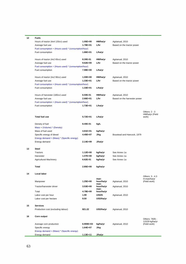
63
12 Fuels
Hours of tractor (4x4 120cv) used 1.05E+00 HM/ha/yr Agrianual, 2010
Average fuel use 1.78E+01 L/hr Based on the tractor power
Fuel consumption = (Hours used) * (consumption/hour)
Fuel consumption 1.86E+01 L/ha/yr
Hours of tractor (4x2 65cv) used 8.30E-01 HM/ha/yr Agrianual, 2010
Average fuel use 9.62E+00 L/hr Based on the tractor power
Fuel consumption = (Hours used) * (consumption/hour)
Fuel consumption 7.98E+00 L/ha/yr
Hours of tractor (4x2 90cv) used 1.00E+00 HM/ha/yr Agrianual, 2010
Average fuel use 1.33E+01 L/hr Based on the tractor power
Fuel consumption = (Hours used) * (consumption/hour)
Fuel consumption 1.33E+01 L/ha/yr
Hours of harvester (180cv) used 6.50E-01 HM/ha/yr Agrianual, 2010
Average fuel use 2.66E+01 L/hr Based on the harvester power
Fuel consumption = (Hours used) * (consumption/hour)
Fuel consumption 1.73E+01 L/ha/yr
Total fuel use 5.72E+01 L/ha/yr
Others: 2 - 3 HM/ha/yr (Field work)
Density of fuel 8.40E-01 kg/L
Mass = (Volume) * (Density)
Mass of fuel used 4.81E+01 kg/ha/yr
Specific energy of diesel 4.45E+07 J/kg Boustead and Hancock, 1979
Energy demand = (Mass) * (Specific energy)
Energy demand 2.14E+09 J/ha/yr
13 Steel
Tractors 1.12E+00 kg/ha/yr See Annex 1a
Harvester 1.07E+00 kg/ha/yr See Annex 1a
Agricultural Machinery 6.62E-01 kg/ha/yr See Annex 1a
Total 2.85E+00 kg/ha/yr
14 Local labor
Manpower 1.25E+00 man-hour/ha/yr Agrianual, 2010
Others: 3 - 4.3 H-man/ha/yr (Field work)
Tractor/harvester driver 3.53E+00 man-hour/ha/yr Agrianual, 2010
Total 4.78E+00 man-hour/ha/yr
Labor cost per hour 1.99 USD/h Agrianual, 2010
Labor cost per hectare 9.50 USD/ha/yr
15 Services
Production cost (excluding labour) 821.22 USD/ha/yr Agrianual, 2010
16 Corn output
Average corn production 6.900E+03 kg/ha/yr Agrianual, 2010
Others: 7605 -11529 kg/ha/yr (Field work)
Specific energy 1.64E+07 J/kg
Energy demand = (Mass) * (Specific energy)
Energy demand 1.13E+11 J/ha/yr

64
Annex 1a: Calculation notes for agricultural machinery in corn production
Description Weight (kg)
Life spam (h)
Hours used (h/ha/yr)
Ref. for hours used
Machinery used up (kg/ha/yr)
Tractor tires 90cv 3870 10000 1.00 Agrianual, 2010 0.39
Tractor tires 120cv 4920 10000 1.05 Agrianual, 2010 0.52
Tractor tires 65cv 2580 10000 0.83 Agrianual, 2010 0.21
Harvester 16400 10000 0.65 Agrianual, 2010 1.07
Moldboard plowing 3200 8000 0.40 Agrianual, 2010 0.16
Limestone sprayer 1203 8000 0.33 Agrianual, 2010 0.05
Seeder 1500 8000 0.65 Agrianual, 2010 0.12
Seed mixer 800 8000 0.10 Agrianual, 2010 0.01
Field cultivator 850 8000 0.50 Agrianual, 2010 0.05
Agrochemical sprayer 2140 8000 1.00 Agrianual, 2010 0.27
Annex 1b: Local emissions in corn production
Nitrogen application (urea)
N2O 1.325 % of N in fert. is conv. in N2O
(IPCC, 2006) 1.08 kgN2O/ha/yr
CO2 0.2 kgC/kgurea (IPCC, 2006) 88.00 kgCO2/ha/yr
Lime
CO2 0.13 kgC/kglime (IPCC, 2006) 166.83 kgCO2/ha/yr
Diesel
CO2 Stoichiometric value 152.10 kgCO2/ha/yr

65
Annex 2. Calculation notes for soybean production system
Note Description Value Unit References Other estimates (if any)
1 Sun
Insolation 1.86E+06 watt-hour/m2/yr http://eosweb.larc.nasa.gov/cgi-bin/sse/sse.cgi
Albedo 14% http://eosweb.larc.nasa.gov/cgi-bin/sse/sse.cgi
Conversion 3.60E+03 J/Wh
Insolation energy = (1-Albedo) * (Insolation) * (3600 J/kWh)
Insolation energy 5.77E+09 J/m2/yr
Cropped area 1.00E+04 m2/ha
Insolation energy = (Land area) * (Insolation)
Insolation energy 5.77E+13 J/ha/yr
2 Rain
Precipitation (Average years 1961-1990, Maringa city) 1.80E+03
mm/yr or L/m2/yr http://eosweb.larc.nasa.gov/cgi-bin/sse/sse.cgi
Cropped area 1.00E+04 m2/ha
Density of water 1.00E+00 kg/L
Mass of rain = (Precipitation) * (Area) * (Density)
Mass of rain 1.80E+07 kg/ha/yr
Fraction of water that is evapotranspired 62% www.inmet.gov.br
Mass of rain evapotranspired 1.12E+07 kg/ha/yr
Free energy of water = (Evapotranspired water) * (Gibbs free energy of water)
Gibbs free energy of water 4.94E+03 J/kg Odum, 1996
Energy of rain 5.52E+10 J/ha/yr
3 Deep heat
Heat flow through earth crust
Average heat flow per area 1.00E+06 J/m2/yr Odum, 1996
Land area 1.00E+04 m2/ha
Energy = (Land area) * (Heat flow per area)
Energy 1.00E+10 J/yr
4 Soil loss
Soil loss (eroded) 1.70E+04 kg/ha/yr http://www.fea.unicamp.br/docentes/ortega/livro/C17-EAnaliseAl-JM.pdf (pg 9)
Ratio of the organic matter in the soil 4% Organic matter in soil is reported in the range 3-6% of total soil weigh (Odum,1996)
Organic matter in topsoil used up = (Mass of topsoil) * (% organic matter)
Organic matter in topsoil used up 6.80E+02 kg/ha/yr
Water content in organic matter 70% Average value
Dry organic matter lost with erosion = (Organic matter) * (1-Water content)
Dry organic matter lost with erosion 2.04E+02 kgdw/ha/yr
Energy content of dry organic matter 5.40E+03 Kcal/kgdw Odum, 1996
Energy = (kgdw/ha/yr) * (5400 Kcal/kgdw) * (4186 J/Kcal)
Energy content of dry organic matter 4.61E+09 J/ha/yr
5 Limestone
Limestone use 2.00E+02 kg/ha/yr Agrianual, 2010
Others: 1200 kg/ha/yr (Hirakuri, 2008); 413 kg/ha/yr (field work)
Specific energy 6.11E+05 J/kg Odum, 1996
Energy demand = (Mass) * (Specific energy)
Energy demand 1.22E+08 J/ha/yr

66
6 Agrochemicals
Other chemicals 1.10E+00 kg/ha/yr Agrianual, 2010
Herbicides 5.45E+00 kg/ha/yr Agrianual, 2010
Insecticides 2.95E+00 kg/ha/yr Agrianual, 2010
Fungicides 9.60E-01 kg/ha/yr Agrianual, 2010
Total 1.05E+01 kg/ha/yr
Others: 7,14 kg/ha/yr (Hirakuri, 2008); 13,2 kg/ha/yr (Field work)
7 Seeds
Mass of seeds used 6.50E+01 kg/ha/yr Agrianual, 2010
Others: 56 kg/ha/yr (Hirakuri, 2008); 82,3 kg/ha/yr (Field work)
8 Organic fertilizer
Total organic fertilizer (pig manure) used 1.03E+03 kg/ha/yr From field work
Nitrogen in manure 5,82E+00 kg/ha/yr Cederberg and Flysjö, 2004
Phosphorous in manure 2,02E+00 kg/ha/yr Cederberg and Flysjö, 2004
Potassium in manure 2,36E+00 kg/ha/yr Cederberg andFlysjö, 2004
9 Nitrogen fertilizer
NPK fertilizer used (0-20-20) 3.00E+02 kg/ha/yr Agrianual, 2010
% N 0% Agrianual, 2010
N = (Total fertilizer) * (%N)
Annual N use 0.00E+00 kg N/ha/yr
10 Phosphate fertilizer
NPK fertilizer used (0-20-20) 3.00E+02 kg/ha/yr Agrianual, 2010
% P2O5 20% Agrianual, 2010
P = (Total fertilizer) * (%P2O5)
Annual P2O5 use 6.00E+01 kg P/ha/yr
11 Potassium fertilizer
NPK fertilizer used (0-20-20) 3.00E+02 kg/ha/yr Agrianual, 2010
% K2O 20% Agrianual, 2010
K = (Total fertilizer) * (%K2O)
Annual K2O use 6.00E+01 kg K/ha/yr
12 Fuels
Hours of tractor (4x4 120cv) used 6.70E-01 HM/ha/yr Agrianual, 2010
Average fuel use 1.78E+01 L/hr Based on the tractor power
Fuel consumption = (Hours used) * (consumption/hour)
Fuel consumption 1.19E+01 L/ha/yr
Hours of tractor (4x2 65cv) used 4.50E-01 HM/ha/yr Agrianual, 2010
Average fuel use 9.62E+00 L/hr Based on the tractor power
Fuel consumption = (Hours used) * (consumption/hour)
Fuel consumption 4.33E+00 L/ha/yr
Hours of tractor (4x2 90cv) used 1.20E+00 HM/ha/yr Agrianual, 2010
Average fuel use 1.33E+01 L/hr Based on the tractor power
Fuel consumption = (Hours used) * (consumption/hour)
Fuel consumption 1.60E+01 L/ha/yr
Hours of harvester (180cv) used 6.50E-01 HM/ha/yr Agrianual, 2010
Average fuel use 2.66E+01 L/hr Based on the harvester power
Fuel consumption = (Hours used) * (consumption/hour)
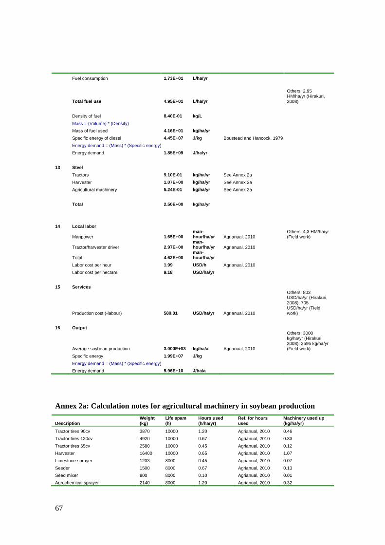
67
Fuel consumption 1.73E+01 L/ha/yr
Total fuel use 4.95E+01 L/ha/yr
Others: 2,95 HM/ha/yr (Hirakuri, 2008)
Density of fuel 8.40E-01 kg/L
Mass = (Volume) * (Density)
Mass of fuel used 4.16E+01 kg/ha/yr
Specific energy of diesel 4.45E+07 J/kg Boustead and Hancock, 1979
Energy demand = (Mass) * (Specific energy)
Energy demand 1.85E+09 J/ha/yr
13 Steel
Tractors 9.10E-01 kg/ha/yr See Annex 2a
Harvester 1.07E+00 kg/ha/yr See Annex 2a
Agricultural machinery 5.24E-01 kg/ha/yr See Annex 2a
Total 2.50E+00 kg/ha/yr
14 Local labor
Manpower 1.65E+00 man-hour/ha/yr Agrianual, 2010
Others: 4,3 HM/ha/yr (Field work)
Tractor/harvester driver 2.97E+00 man-hour/ha/yr Agrianual, 2010
Total 4.62E+00 man-hour/ha/yr
Labor cost per hour 1.99 USD/h Agrianual, 2010
Labor cost per hectare 9.18 USD/ha/yr
15 Services
Production cost (-labour) 580.01 USD/ha/yr Agrianual, 2010
Others: 803 USD/ha/yr (Hirakuri, 2008); 705 USD/ha/yr (Field work)
16 Output
Average soybean production 3.000E+03 kg/ha/a Agrianual, 2010
Others: 3000 kg/ha/yr (Hirakuri, 2008); 3595 kg/ha/yr (Field work)
Specific energy 1.99E+07 J/kg
Energy demand = (Mass) * (Specific energy)
Energy demand 5.96E+10 J/ha/a
Annex 2a: Calculation notes for agricultural machinery in soybean production
Description Weight (kg)
Life spam (h)
Hours used (h/ha/yr)
Ref. for hours used
Machinery used up (kg/ha/yr)
Tractor tires 90cv 3870 10000 1.20 Agrianual, 2010 0.46
Tractor tires 120cv 4920 10000 0.67 Agrianual, 2010 0.33
Tractor tires 65cv 2580 10000 0.45 Agrianual, 2010 0.12
Harvester 16400 10000 0.65 Agrianual, 2010 1.07
Limestone sprayer 1203 8000 0.45 Agrianual, 2010 0.07
Seeder 1500 8000 0.67 Agrianual, 2010 0.13
Seed mixer 800 8000 0.10 Agrianual, 2010 0.01
Agrochemical sprayer 2140 8000 1.20 Agrianual, 2010 0.32

68
Annex 2b: Local emissions in soybean production
Nitrogen application (urea)
N2O 1.325 % of N in fert. is conv. in N2O
(IPCC, 2006) 0.00 kgN2O/ha/yr
CO2 0.2 kgC/kgurea (IPCC, 2006) 0.00 kgCO2/ha/yr
Lime (IPCC, 2006)
CO2 0.13 kgC/kglime (IPCC, 2006) 95.33 kgCO2/ha/yr
Diesel
CO2 Stoichiometry 131.55 kgCO2/ha/yr

69
Annex 3. Calculation notes for pig production system
Note Description Value Unit References Other estimates (if any)
1 Sun
Insolation 1.86E+06 watt-hour/m2/yr http://eosweb.larc.nasa.gov/cgi-bin/sse/sse.cgi
Albedo 1.40E-01 http://eosweb.larc.nasa.gov/cgi-bin/sse/sse.cgi
Conversion 3.60E+03 J/Wh
Insolation energy = (1-Albedo) * (Insolation) * (3600 J/kWh)
Insolation energy 5.77E+09 J/m2/yr
Cropped area 8.74E+02 m2 Angonese et al., 2006
Insolation energy = (Land area) * (Insolation)
Insolation energy 5.04E+12 J/yr
Insolation energy 7.06E+07 J/kg pig
2 Rain
Precipitation (Average years 1961-1990, Maringa city)
1.80E+03 mm/yr or L/m2/yr
http://eosweb.larc.nasa.gov/cgi-bin/sse/sse.cgi
Cropped area 8.74E+02 m2 Angonese et al., 2006
Density of water 1.00E+00 kg/L
Mass of rain = (Precipitation) * (Area) * (Density)
Mass of rain 1.58E+06 kg/yr
Fraction of water that is evapotranspired 62% www.inmet.gov.br
Mass of rain evapotranspired 9.77E+05 kg/yr
Free energy of water = (Evapotranspired water) * (Gibbs free energy of water)
Gibbs free energy of water 4.94E+03 J/kg Odum, 1996
Energy of rain 4.83E+09 J/yr
Energy of rain 6.75E+04 J/kg pig
3 Deep heat
Heat flow through earth crust
Average heat flow per area 1.00E+06 J/m2/yr Odum, 1996
Land area 8.74E+02 m2 Angonese et al. 2006
Energy = (Land area) * (Heat flow per area)
Energy 8.74E+08 J/yr
Energy 1.22E+04 J/kg pig
4 Water (groundwater)
Water use 936000 L/yr From field work (Itaipu data)
Gibbs free energy of water 4.94E+03 J/kg Odum, 1996
Energy of water = (Consumption) * (Gibbs free energy of water)
Energy 4.62E+09 J/yr
Energy 6.47E+04 J/kg pig
Water use 1.31E+01 kg/kg pig
5 Feed
Total feed use 1.64E+05 kg/yr Angonese et al., 2006
Pig feed composition From field work
Corn - 80% 1.31E+05 kg/yr
1.84E+00 kg/kg pig
Soy meal - 17% 2.79E+04 kg/yr
3.90E-01 kg/kg pig
Other nutrients - 3% 4.92E+03 kg/yr
6.88E-02 kg/kg pig

70
6 Electricity
Electricity use 1.10E+02 kWh/yr Angonese et al., 2006
Conversion factor 3.60E+06 J/kWh
Electricity use 3.95E+08 J/yr
Electricity use 5.53E+03 J/kg pig
Electricity use 1.54E-03 kWh/kg pig
7 Local labor
Labor per year 5.16E+03 man-hour/yr
Labor cost per hour 1.99 USD/h Anualpec, 2010
Labor cost per hectare 10261 USD/yr Anualpec, 2010
Labor cost per hectare 0.144 USD/kg pig
Labor 7.22E-02 man-hour/kg pig
8 Services
Production cost (-labour) 87236 USD/yr Anualpec, 2010
Production cost (-labour) 1.220 USD/kg pig
9 Output
Meat production 7.150E+04 kg/yr Angonese et al., 2006
Specific energy 9.21E+06 J/kg pig Angonese et al., 2006
Energy demand = (Mass) * (Specific energy)
Energy demand 6.59E+11 J/yr
Manure 4.212E+05 kg/yr Angonese et al., 2006
5.89E+00 kg/kg pig
Annex 3a: Parameters for pig production
Parameters Value Unit Ref.
US Dollar/ Br Real 0.54
Average number of pigs produced per year per farm 650 pigs Angonese et al., 2006
Breeding time 120 days/year Angonese et al., 2006
Pig weight after 120 days 110 kg/pig Angonese et al., 2006
Annex 3b: Local emissions from manure management in the pig production
Ammoniaa 14% Of total N in manure
0.0056 kgNH3/kgpig
Nitrous oxidea 0.02 kg N in N2O per kg N (after ammonia losses)
0.0009 kgN2O/kgpig
Methane a (entheric fermantation and manure management)
3.58 kgCH4/pig/yr 0.0325 kgCH4/kgpig
aBased on data from Cederberg and Flysjö (2004).

71
Authors’ biographical sketch
Pier Paolo Franzese (Italian) has a permanent position as Senior Researcher in Ecology
at Parthenope University of Naples, Italy. At the Faculty of Science and Technology of
the same university, Dr. Franzese also holds the position of Assistant Professor of
Environmental and Energy Assessment. After graduating with honours in
Environmental Sciences, he achieved the title of International Ph.D. in “Crop Systems,
Forestry and Environmental Science” with orientation in Environmental Science and
label of Doctor Europaeus. Dr. Franzese is founder member of the International Ph.D.
Programme “Environment, Resources, and Sustainable Development” hosted at
Parthenope University where he also founded and is now directing the Laboratory of
Ecodynamics and Sustainable Development.
Otávio Cavalett (Brazilian) has a PhD in “Food Engineering” from the State University
of Campinas (Brazil). At present he is Researcher in Technological Assessment at the
Brazilian Bioethanol Science and Technology Laboratory (CTBE) that integrates the
Brazilian Center of Research in Energy and Materials (CNPEM). Currently he is
working on environmental assessment tools, sustainable bioethanol production
technologies, and biorefinery systems.
Tiina Häyhä (Finnish) has a Master of Science in Economics and Business
Administration from the University of Jyväskylä (Finland). Currently she is a PhD
student in the International PhD Programme “Environment, Resources, and Sustainable
Development” hosted at Parthenope University of Naples (Italy) where she is working
on ecosystem services assessment, multi-criteria environmental assessment, and energy-
related issues.
Salvatore D’Angelo (Italian) has a degree in Economics and two Masters degrees in
“Economics and Finance” and “Cooperation and Sustainable Development”. Currently
he is a PhD candidate in “Environment, Resources, and Sustainable Development”.
Before working for the Italian Ministry for the Environment (2001-2004), Mr.
D’Angelo collaborated with the Directorate-General for Economic and Financial Affairs
(DG ECFIN) of the European Commission and the OECD-LEED Programme (LEED
Programme - Local Economic and Employment Development). Since 2005, he has
worked for the Groundwater Section of the UNESCO International Hydrological
Programme, where he is in charge of the “Water Programme for Environmental
Sustainability”.

UNESCO-IHP Water Programme for Environmental Sustainability, Climate Change and Human Impacts
on the Sustainability of Groundwater Resources: Quantity and Quality Issues, Mitigation and Adaptation Strategies in Brazil
Integrated Environmental Assessment of Agricultural and Farming
Production Systems in the Toledo River Basin (Brazil)
ISBN 978-92-3-001138-3