Embed Size (px)
Citation preview
1
Integrated Design of Mechanical Structure and Control Algorithm for Closed-Chain Five-Bar Mechanism
F. X. Wu1, Q. Li 2, W. J. Zhang3, and P. R. Ouyang
Department of Mechanical Engineering
University of Saskatchewan, Saskatoon, SK S7N 5A9, Canada
1On the special leave from Northwestern Ploytechnical University, Xi'an, China 2On the special leave from Department of Mechanical Engineering, University of Adelaide,
Australia 3The corresponding author
Abstract: In the traditional mechatronic systems, the controller designs are usually separated
from the mechanical structure designs. Consequently, the controller algorithms become more and
more complex, i.e., from the PD controller, to the computed-torque controller, and to all sorts of
the adaptive controller. These complex control algorithms encounter many difficulties in
implementation of the control algorithms to closed-chain mechanisms. The main reason for these
difficulties is the so-called computational overhead with the dynamic model of the closed-chain
mechanisms. The computational overhead is even experienced in a parallel manipulator system
(one of the closed-chain types). One of the solutions to this problem is to seek a smart design of
mechanical structures based on the methodology called Design For Control (DFC). DFC
specifically proposes the procedure, i.e., design of a mechanical structure, simplification of the
dynamic model of the mechanical structure, and design of a simple control algorithm (such as
PD controller). In this paper, a 2-dof five-bar closed-chain mechanism (called Delta mechanism
for short) is studied. It is shown that the smart design of the mechanical structure of the Delta
mechanism can lead to some configuration invariants in the dynamic model. Therefore, the
design of PD controllers, incorporating these invariants, can achieve excellent system
performance.
Keyword: DFC, five-bar mechanism, control algorithm, tracking performance
2
1. Introduction
Robot manipulators may be classified into two categories in terms of their architecture. In the
first category, all of the links in the kinematics chain are connected sequentially starting from a
fixed base. The last link in the chain is connected from one end to a previous link but is free from
the other end resulting in an open link chain. We refer to these systems as “opened kinematics
chain” . Typically, in these systems each link is connected to the previous link in the link chain
by a joint and all of the joints are actuated. In the robotics literature, this kind of open chain
systems is usually called “serial robots” . In the second category, the links in the kinematics chain
are connected in series as well as in parallel combinations forming one or more closed-link
loops. We refer to these mechanisms as “closed-chain systems”. Typically, in these systems not
all joints in closed-chain mechanisms are actuated. In the robotics literature, this kind of closed-
chain system is usually called “parallel robots” . The simplest characterization of this category is
that of the so-called fully parallel robots which consist of a set of serial links each connected to a
fixed base from one end, and connected to a common moving endpoint (or platform) on the other
end, and resulting in a closed-chain mechanism, for example, steward platform [1].
During the last two decades, the serial robot control has been a long-standing field. Since the
serial robots are governed by a well-established formulation of the equations of motion [4,5],
which possess many excellent properties, a lot of control results [4-8] have been developed for
them. When the structure parameters of the serial robots are known exactly, the PD controller
applied to the regulation problem, and the computed-torque controller applied to the trajectory
tracking problem [4,5] are widely employed. To deal with the uncertainties in the structure
parameters of the serial robots, Craig [6] developed an adaptive controller based on computed-
torque control, and Soltine and Li [7] developed another adaptive controller based on passive
property. The readers are invited to see the literatures [5,8] for all sorts of controllers applied to
serial robots. However, the open-chain mechanisms possess some inherent disadvantages, for
example, the position accuracy at the endpoint of the long robot arm is considerably low; a small
amount of error at each revolution joint is magnified at the endpoint of arm as its length gets
longer; most importantly, the mechanical stiffness of the open-chain construction is inherently
poor since each joint is equipped with an actuator. As a result, the accuracy of motion tracking
3
performance can be deteriorated. The research trend in modern machinery development therefore
shifts toward the parallel robots for the position and the trajectory tracking purpose.
The equations of motion governing the parallel robots are the same in form as the equations of
motion governing the serial robots, and also possess almost the same properties. It seems that all
control methods in the serial robots may apply to the parallel robot control. Nevertheless,
because they are local and implicit, the equations of motion of the parallel robots include more
structure parameters and are of more complexity than those of the serial robots with the same
degree of freedoms (dof). This results in the computation complexity in designing a controller.
Several methods reported in the literature were proposed to design the controller for parallel
robots [9-11]. As suggested by Lin and Chen [9], a very complex control structure that is
composed of several sub-control algorithms, such as a model reference adaptive control, a
disturbance compensation loop, with a modified switching controller plus some feedback loops,
was proposed to control the four-bar-link mechanism to follow a pre-specified trajectory.
Ghorbel [10,11] presented the PD control with simple gravity compensation for a two-dof
closed-chain mechanism for the point-to-point control task. Although Ghorbel’s controller is the
same in form as the controller used for the open-closed robot, the complexity of its computation
is by far more. In general, the intensive computation can result in the difficulty in physical realiz-
ation of a controller for high-speed performance. There is indeed a trend to apply a parallel
computation/processing technique [12] for controlling parallel mechanism systems with multi-
dof.
Another method to overcome computation complexity is to design the mechanical structure for a
relatively simpler dynamic model. Comparing with serial robots, the dynamical model of the
parallel robot includes more structure parameters. Therefore, more opportunities are present for
the judicious selection of these parameters. Along this line of thinking, Asada and Toumi [13,14]
designed a parallel drive five-bar mechanism. One of the most advantageous properties for this
mechanism is that its mass matrix is configuration-invariant, and thus, it is a time-invariant
diagonal matrix. This consequently leads to the cancellation of the centrifugal and Coriolis
terms. They demonstrated that the design of the controller was simpler, and the performance of
the closed-loop system was improved. Following Toumi’s design strategy, Diken [15] improved
4
the motion tracking performance of an open-loop robot manipulator by applying a mass
redistribution scheme. In his study, the structure of a robot arm was first reduced into
dynamically equivalent point masses so as to eliminate the gravitational term in the dynamic
model. A simple algorithm was then applied to control the system for satisfactory performance
of trajectory tracking.
Recently, a more general concept called “Design For Control (DFC)” was proposed [2,16]. The
essence of the concept suggests designing the mechanical structure of a programmable machine
by fully exploring the physical understanding of overall system with its consideration of
facilitation of controller design as well as the execution of control action with the least hardware
restriction. An intuitive way to realize this objective is to design an appropriate structure for the
mechanical part such that it can result in a “simple” dynamic model and thus a more predictable
dynamic response. The four-bar-link mechanism was studied and the gravitational term in the
dynamic model was cancelled by using complete shaking force balancing scheme. In essence,
this methodology makes the center of general mass of the mechanism configuration-invariant by
mass redistribution design. Further results of the four-bar-link mechanism based on DFC were
reported in [17].
From the discussion above, it can be seen that the studies in [2,16] took advantage of the
property called configuration-invariance of potential energy (CIPE), while the studies in [13,14]
took advantage of the property called configuration-invariance of generalized inertial (CIGI).
Note that both partial CIPE and partial CIGI are possible (PCIGE and PCIGI for short,
respectively). The motivation of this paper is to investigate what effects could be on system
performances by integrating CIPE and PCIGI. Based on this motivation, a study taking a closed-
loop five-bar mechanism with 2-dof was made, and will be presented in this paper. Section 2
describes the dynamic model of a 2-dof closed-chain five-bar mechanism, which gives a
foundation for both mechanical structure design and controller design. In Section 3, synthesis of
the mass redistribution design is presented to derive configuration-invariant properties. In
Section 4, the controller design and simulations are presented. In Section 5, a conclusion is
drawn.
5
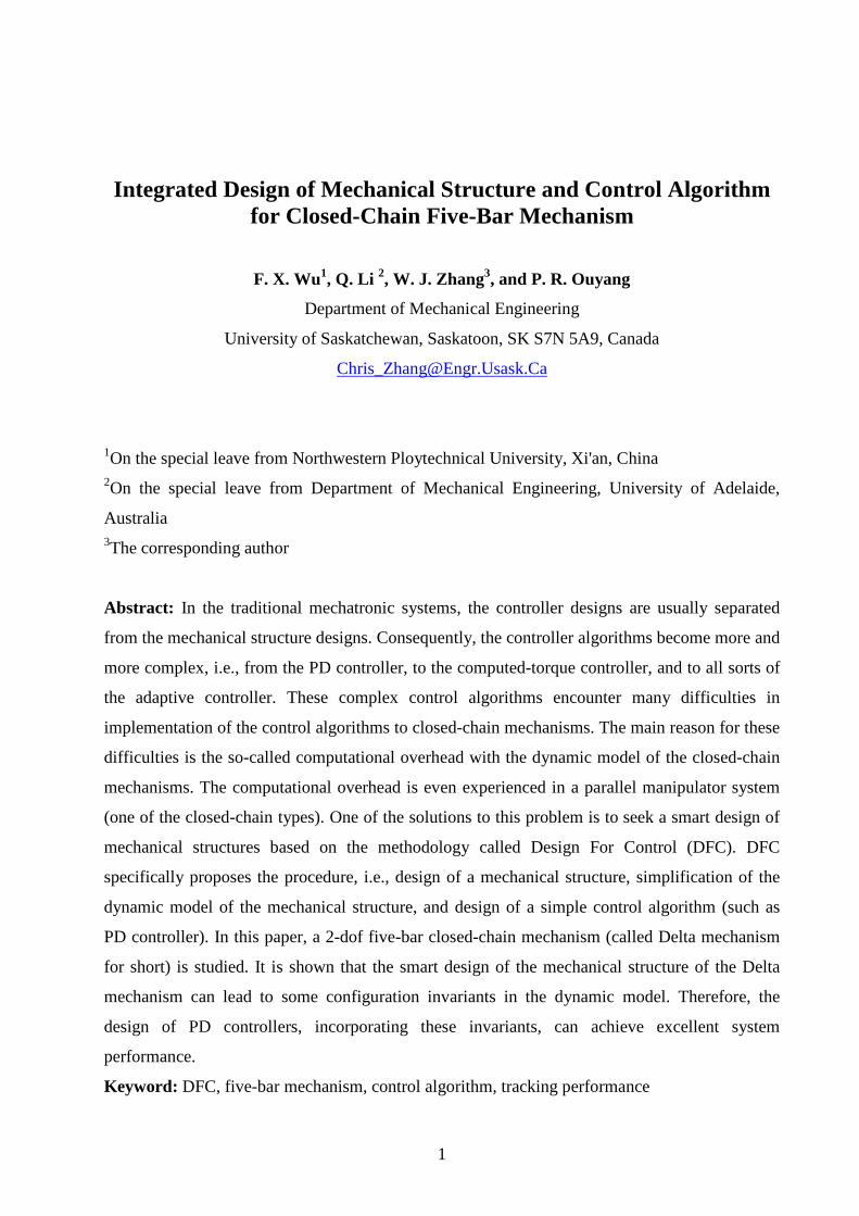
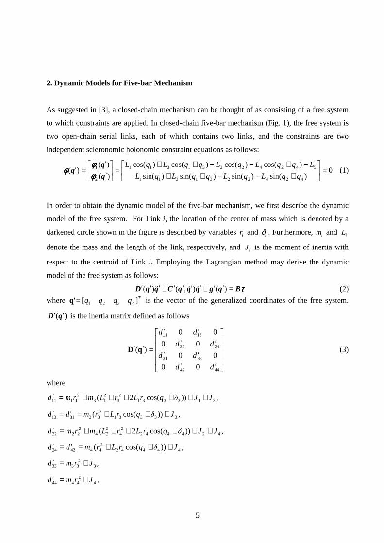
2. Dynamic Models for Five-bar Mechanism
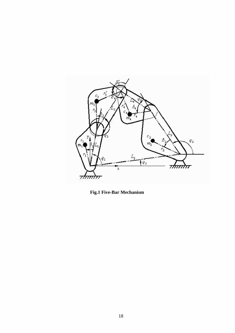
As suggested in [3], a closed-chain mechanism can be thought of as consisting of a free system
to which constraints are applied. In closed-chain five-bar mechanism (Fig. 1), the free system is
two open-chain serial links, each of which contains two links, and the constraints are two
independent scleronomic holonomic constraint equations as follows:
0)sin()sin()sin()sin(
)cos()cos()cos()cos(
)(
)()(
4242231311
54242231311
2
1 =
+−−++
−+−−++=
′′
=′qqLqLqqLqL
LqqLqLqqLqL
q
φφφφφφφφ
φφφφ (1)
In order to obtain the dynamic model of the five-bar mechanism, we first describe the dynamic
model of the free system. For Link i, the location of the center of mass which is denoted by a
darkened circle shown in the figure is described by variables ri and δi . Furthermore, mi and Li
denote the mass and the length of the link, respectively, and Ji is the moment of inertia with
respect to the centroid of Link i. Employing the Lagrangian method may derive the dynamic
model of the free system as follows:
ττττBqgqqqCqqD =′′+′′′′+′′′ )(),()( &&&& (2)
where Tqqqq ][' 4321=q is the vector of the generalized coordinates of the free system.
)(qD ′′ is the inertia matrix defined as follows
′′′′
′′′′
=′′
4442
3331
2422
1311
00
00
00
00
)(
dd
dd
dd
dd
qD (3)
where
3133312
3213
21111 ))cos(2( JJδqrLrLmrmd ++++++=′ ,
333312
333113 ))cos(( JδqrLrmdd +++=′=′ ,
4244422
4224
22222 ))cos(2( JJδqrLrLmrmd ++++++=′ ,
444422
444224 ))cos(( JδqrLrmdd +++=′=′ ,
32
3333 Jrmd +=′ ,
42
4444 Jrmd +=′ ,
6
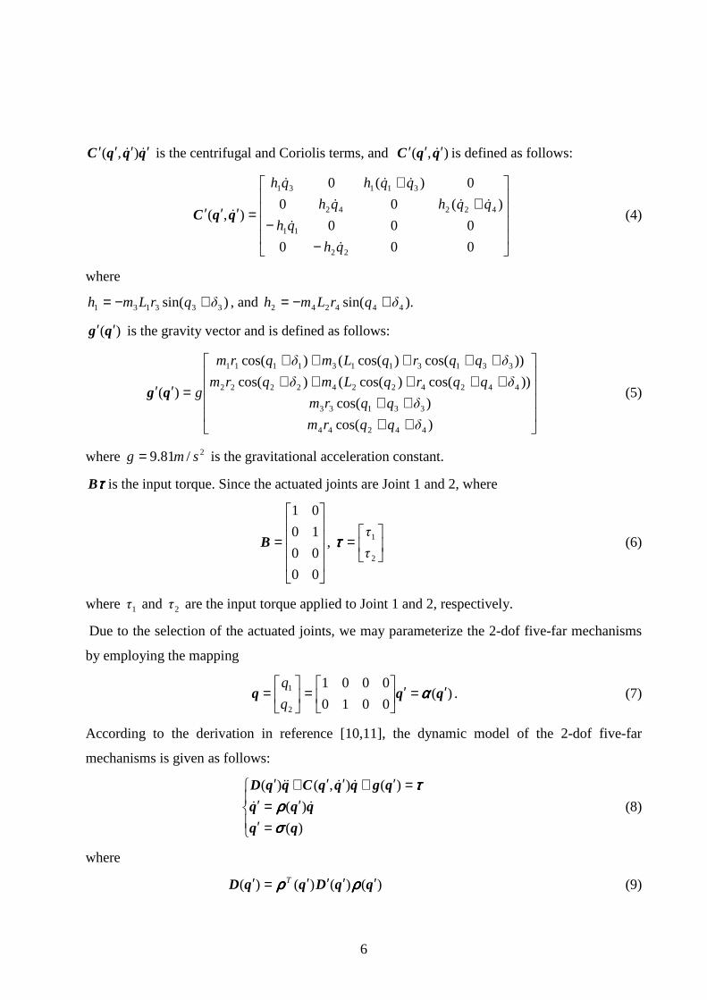
qqqC && ′′′′ ),( is the centrifugal and Coriolis terms, and ),( qqC &′′′ is defined as follows:
−−
++
=′′′
000
000
)(00
0)(0
),(
22
11
42242
31131
qh
qh
qqhqh
qqhqh
&
&
&&&
&&&
&qqC (4)
where
)sin( 333131 δqrLmh +−= , and ).sin( 444242 δqrLmh +−=
)(qg ′′ is the gravity vector and is defined as follows:
++++
++++++++++
=′′
)cos(
)cos(
))cos()cos(()cos(
))cos()cos(()cos(
)(
44244
33133
44242242222
33131131111
δqqrm
δqqrm
δqqrqLmδqrm
δqqrqLmδqrm
gqg (5)
where 2/81.9 smg = is the gravitational acceleration constant.
ττττB is the input torque. Since the actuated joints are Joint 1 and 2, where
=
00
00
10
01
B ,
=
2
1
τ
τττττ (6)
where 1τ and 2τ are the input torque applied to Joint 1 and 2, respectively.
Due to the selection of the actuated joints, we may parameterize the 2-dof five-far mechanisms
by employing the mapping
)(0010
0001
2
1 qqq ′=′
=
= ααααq
q. (7)
According to the derivation in reference [10,11], the dynamic model of the 2-dof five-far
mechanisms is given as follows:
=′′=′
=′+′′+′
)(
)(
)(),()(
qqq
qgqqqCqqD
σσσσρρρρ
ττττ&&
&&&&
(8)
where
)()()()( qqDqqD ′′′′=′ ρρρρρρρρ T (9)
7
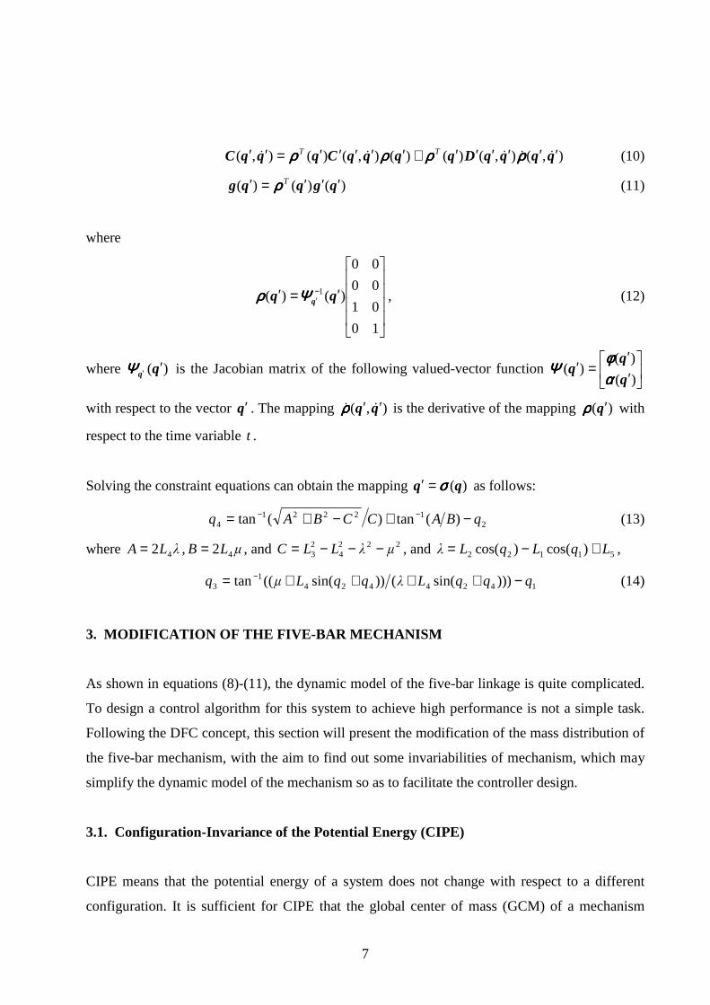
),(),()()(),()(),( qqqqDqqqqCqqqC &&&&& ′′′′′′+′′′′′=′′ ρρρρρρρρρρρρρρρρ TT (10)
)()()( qgqqg ′′′=′ Tρρρρ (11)
where
′=′ −
′
10
01
00
00
)()( 1 qq qΨΨΨΨρρρρ , (12)
where )(qq ′′ΨΨΨΨ is the Jacobian matrix of the following valued-vector function
′′
=′)(
)()(
q
ααααφφφφ
ΨΨΨΨ
with respect to the vector q′ . The mapping ),( qq && ′′ρρρρ is the derivative of the mapping )(q′ρρρρ with
respect to the time variable t .
Solving the constraint equations can obtain the mapping )(qq σσσσ=′ as follows:
212221
4 )(tan)(tan qBACCBAq −+−+= −− (13)
where λLA 42= , µLB 42= , and 2224
23 µλLLC −−−= , and 51122 )cos()cos( LqLqLλ +−= ,
14244241
3 )))sin(())sin(((tan qqqLλqqLµq −++++= − (14)
3. MODIFICATION OF THE FIVE-BAR MECHANISM
As shown in equations (8)-(11), the dynamic model of the five-bar linkage is quite complicated.
To design a control algorithm for this system to achieve high performance is not a simple task.
Following the DFC concept, this section will present the modification of the mass distribution of
the five-bar mechanism, with the aim to find out some invariabilities of mechanism, which may
simplify the dynamic model of the mechanism so as to facilitate the controller design.
3.1. Configuration-Invariance of the Potential Energy (CIPE)
CIPE means that the potential energy of a system does not change with respect to a different
configuration. It is sufficient for CIPE that the global center of mass (GCM) of a mechanism
8
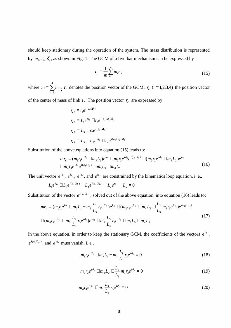
should keep stationary during the operation of the system. The mass distribution is represented
by iii rm δ , , , as shown in Fig. 1. The GCM of a five-bar mechanism can be expressed by
cii
imm
rrc ∑=
=4
1
1 (15)
where ∑=
=4
1iimm ; cr denotes the position vector of the GCM, )4,3,2,1( =icir the position vector
of the center of mass of link i . The position vector cir are expressed by
)(1
11 δδδδ+= qer ic1r
)(313
3131 δ+++= qqq ereL iicr
)(252
22 δδδδ++= qerL icr
)(4254
4242 δ++++= qqq ereLL iicr
Substitution of the above equations into equation (15) leads to:
5453)(
44
2422)(
331311
244
2213311 )()(
LmLmeerm
eLmermeermeLmermmqq
qqqq
+++
++++=+
+
ii
iiiiiicr
δ
δδδ
(16)
The unit vector 1qe i , 2qe i , 3qe i , and 4qe i are constrained by the kinematics loop equation, i. e.,
052)(
4)(
31224131 =−−−+ ++ LeLeLeLeL qqqqqq iiii
Substitution of the vector )( 13 qqe +i , solved out of the above equation, into equation (16) leads to:
54533
3
533
3
4344
)(33
3
224223
3
131311
3434
4232131
)(
)()(
LmLmerL
Lmeer
L
Lmerm
eermL
LLmermeer
L
LmLmermm
q
qqq
+++++
+++−+= +
δδδ
δδδδ
iiii
iiiiiicr
(17)
In the above equation, in order to keep the stationary GCM, the coefficients of the vectors 1qe i ,
)( 42 qqe +i , and 4qe i must vanish, i. e.,
0313
3
131311 =−+ δδ ii er
L
LmLmerm (18)
03233
3
22422 =++ δδ ii erm
L
LLmerm (19)
0343
3
4344 =+ δδ ii er
L
Lmerm (20)
9
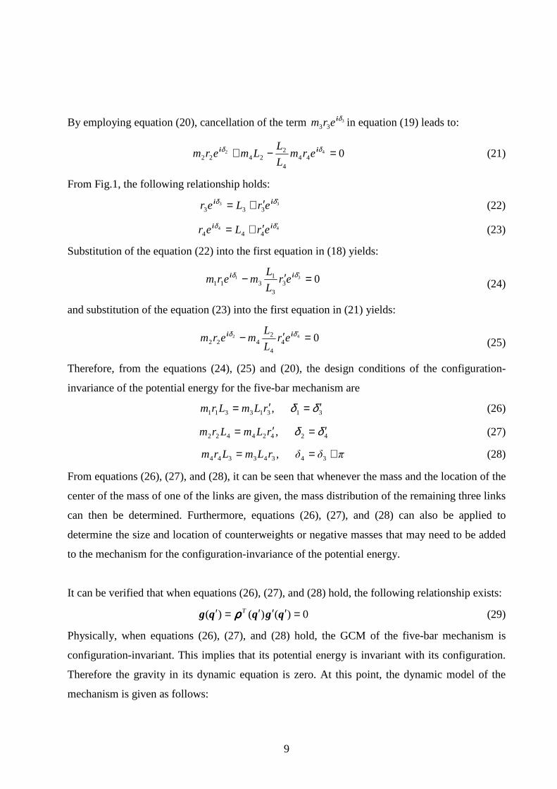
By employing equation (20), cancellation of the term 333
δierm in equation (19) leads to:
04244
4
22422 =−+ δδ ii erm
L
LLmerm (21)
From Fig.1, the following relationship holds:
33333
δδ ′′+= ii erLer (22)
44444
δδ ′′+= ii erLer (23)
Substitution of the equation (22) into the first equation in (18) yields:
0313
3
1311 =′− ′δδ ii er
L
Lmerm (24)
and substitution of the equation (23) into the first equation in (21) yields:
0424
4
2422 =′− ′δδ ii er
L
Lmerm (25)
Therefore, from the equations (24), (25) and (20), the design conditions of the configuration-
invariance of the potential energy for the five-bar mechanism are
31313311 , δδ ′=′= rLmLrm (26)
42424422 , δδ ′=′= rLmLrm (27)
πδ δrLmLrm +== 34343344 , (28)
From equations (26), (27), and (28), it can be seen that whenever the mass and the location of the
center of the mass of one of the links are given, the mass distribution of the remaining three links
can then be determined. Furthermore, equations (26), (27), and (28) can also be applied to
determine the size and location of counterweights or negative masses that may need to be added
to the mechanism for the configuration-invariance of the potential energy.
It can be verified that when equations (26), (27), and (28) hold, the following relationship exists:
0)()()( =′′′=′ qgqqg Tρρρρ (29)
Physically, when equations (26), (27), and (28) hold, the GCM of the five-bar mechanism is
configuration-invariant. This implies that its potential energy is invariant with its configuration.
Therefore the gravity in its dynamic equation is zero. At this point, the dynamic model of the
mechanism is given as follows:
10
ττττ=′′+′ qqqCqqD &&&& ),()( (30)
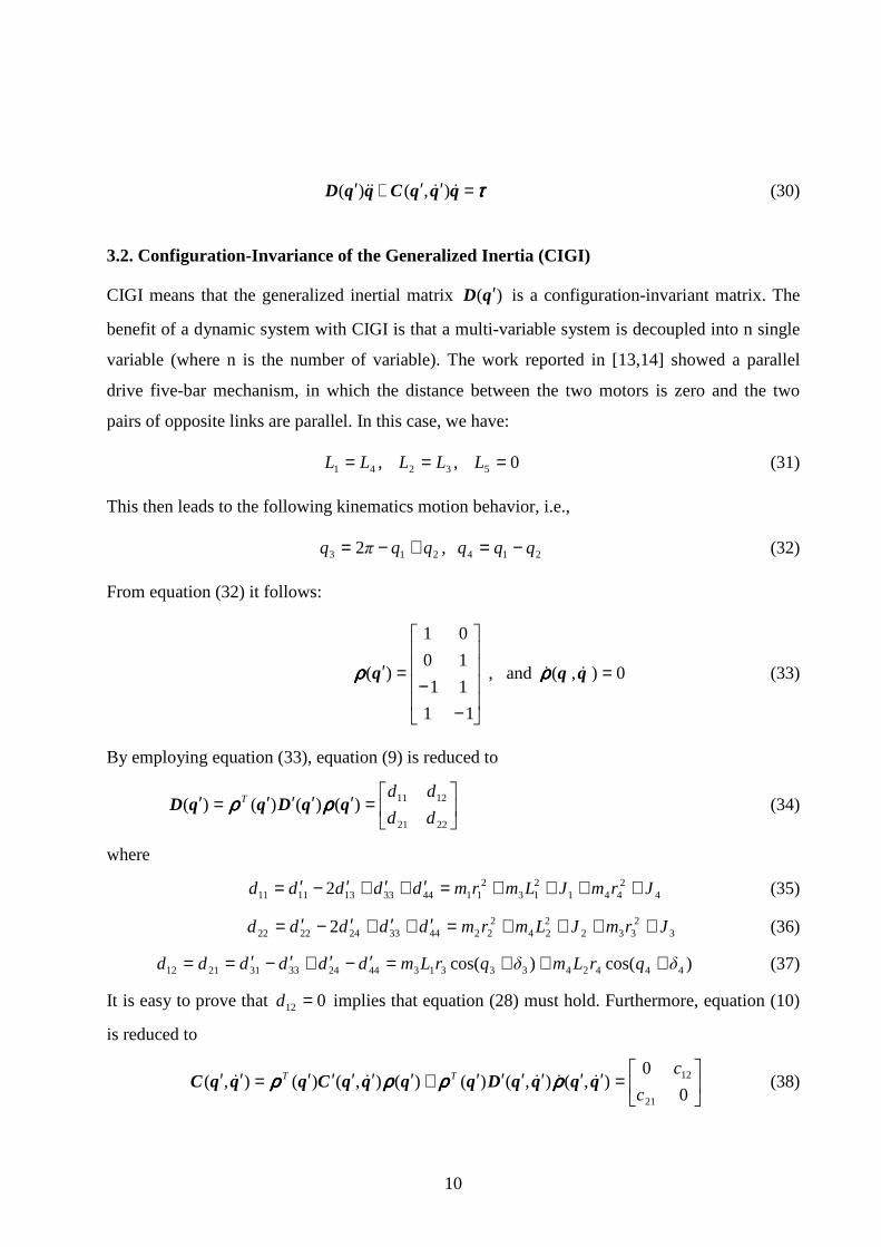
3.2. Configuration-Invariance of the Generalized Inertia (CIGI)
CIGI means that the generalized inertial matrix )(qD ′ is a configuration-invariant matrix. The
benefit of a dynamic system with CIGI is that a multi-variable system is decoupled into n single
variable (where n is the number of variable). The work reported in [13,14] showed a parallel
drive five-bar mechanism, in which the distance between the two motors is zero and the two
pairs of opposite links are parallel. In this case, we have:
41 LL = , 32 LL = , 05 =L (31)
This then leads to the following kinematics motion behavior, i.e.,
213 2 qqπq +−= , 214 qqq −= (32)
From equation (32) it follows:
−−
=′
11
11
10
01
)(qρρρρ , and 0),( =qq &&ρρρρ (33)
By employing equation (33), equation (9) is reduced to
=′′′′=′
2221
1211)()()()(dd
ddT qqDqqD ρρρρρρρρ (34)
where
42
441213
2114433131111 2 JrmJLmrmddddd ++++=′+′+′−′= (35)
32
332224
2224433242222 2 JrmJLmrmddddd ++++=′+′+′−′= (36)
)cos()cos( 4442433313442433312112 δqrLmδqrLmdddddd +++=′−′+′−′== (37)
It is easy to prove that 012 =d implies that equation (28) must hold. Furthermore, equation (10)
is reduced to
=′′′′′′+′′′′′=′′
0
0),(),()()(),()(),(
21
12
c
cTT qqqqDqqqqCqqqC &&&&& ρρρρρρρρρρρρρρρρ (38)
11
where
)cos()( 2242431312 δqrLmrLmc +−= (39)
)cos()( 1142431321 δqrLmrLmc +−−= (40)
It is easy to show that when equation (28) holds:
02112 ≡= cc (41)
Thus the dynamic equation at this point is reduced to:
ττττ=′+ )(qgqD && (42)
where the generalized inertial matrix [ ]2211 dddiag=D is a constant matrix, and 11d and 22d
are defined by equations (35) and (37), respectively.
It may be seen that the conditions for CIPE and CIGI have a overlapping relationship, i.e.,
equation (28). In order that the system possesses both CIPE and CIGI, equations (26)-(28) and
equation (31) must hold simultaneously. In this case, the dynamic equation is further reduced to:
ττττ=qD && (43)
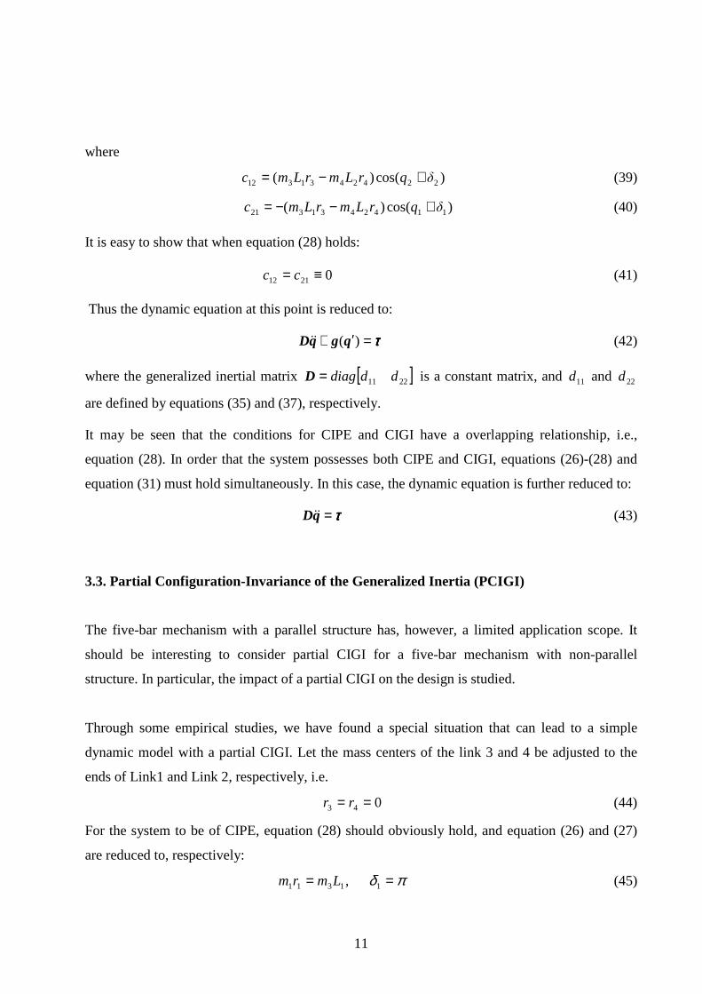
3.3. Partial Configuration-Invariance of the Generalized Inertia (PCIGI)
The five-bar mechanism with a parallel structure has, however, a limited application scope. It
should be interesting to consider partial CIGI for a five-bar mechanism with non-parallel
structure. In particular, the impact of a partial CIGI on the design is studied.
Through some empirical studies, we have found a special situation that can lead to a simple
dynamic model with a partial CIGI. Let the mass centers of the link 3 and 4 be adjusted to the
ends of Link1 and Link 2, respectively, i.e.
043 == rr (44)
For the system to be of CIPE, equation (28) should obviously hold, and equation (26) and (27)
are reduced to, respectively:
πδ == 11311 ,Lmrm (45)
12
πδ == 22422 ,Lmrm (46)
In this situation, the generalized inertia of the free system )(qD ′′ is reduced to a constant matrix,
and the Coriolis/ centripetal matrix of the free system ),( qqC &′′′ is a zero matrix. On the other
hand, when equation (45) holds, the terms related to 3r and 4r in the generalized inertia )(qD ′
are zero, and therefore, the system is partial CIGI (PCIGI). It is further noted that the terms
related to 3r and 4r in )(qD ′ involve trigonometric functions, which cause the generalized
inertial disturbance and may deteriorate the performance of the mechanical system. Therefore the
PCIGI in this case is expected to improve the performance of the system.
4. Controller Design and Simulation Studies
Theoretically, the control algorithms applied to the serial robots, for instance, the computer-
torque control (CTC) method [6], and adaptive control methods based on CTC [6,7], may be
used to the trajectory tracking problems for the parallel robots. The flaw of these algorithms is
that their performance depends heavily on the dynamic model of mechanisms. Comparing with
the serial robots, the dynamic models of the parallel robots are more complicated, so these
algorithms, as anticipated, have encountered some difficulties in implementation.
In the traditional mechatronic systems, the main task was placed on the controller design after
the mechanical structure design, which may be not concurrent, is finished. This caused that the
control algorithms, from the PD control to the CTC to the adaptive control, became more and
more complex. Consequently, the implementing of the controller become more and more
difficult. On contrary, in this section, our idea is that employing the simple controller achieves
the excellent performance for the complex mechanism when the last section has expended more
attention on the mechanical design to reduce the dynamic models of a complex mechanism. The
parallel drive five-bar mechanism with CIPE, whose dynamic equation has been reduced to the
linear time-invariant system described in equation (43), is a special kind of the five-bar
mechanism.
13
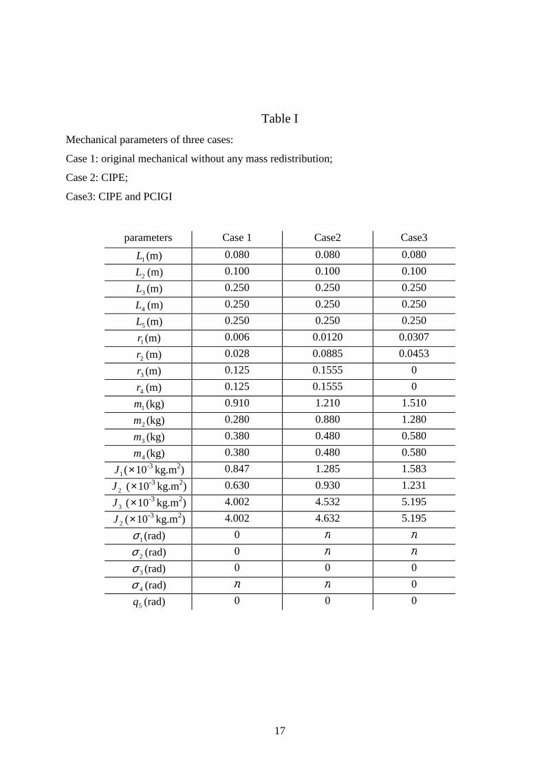
To investigate the effectiveness of our presented method, simulation studies were carried out for
the five-bar mechanism of different cases with different controllers. The parameters of the five-
bar mechanism under different cases are recorded in Table I. Case 1 describes the original
mechanical without any mass redistribution, Case 2 describes the mechanism with only CIPE;
and Case3 describes the mechanism with CIPE and PCIGI. In order to modify easily the existing
mechanism, we employed the added mass method from Case 1, to Case2, and to case3.
In this simulation study, the desired trajectories for two actuated links are expressed as follows:
πtq d 5.01 = , )10156(23
3
4
4
5
5
2fff
d t
t
t
t
t
tπq +−= ,
=d
dd q
q
2
1q (47)
where the scale )(4 st f = is the time span during which the simulation holds.
4.1 Analysis of Simulation 1
In this subsection, we consider tracking performance of the five-bar mechanism of three cases
with the following PD controller:
eKeK dp &+=ττττ (48)
where the vector qqe −= d is the trajectory tracking error, and pK and dK are the gain
matrices and are positive definite. In the simulation, the gain matrices were selected to be
IK p 5= and IK 10=d , where I expresses the second order identity matrix. The motions in
simulation start from 00 =t and end at )(4 st f = , and the initial values are chosen as 0=e and
0=e�
.
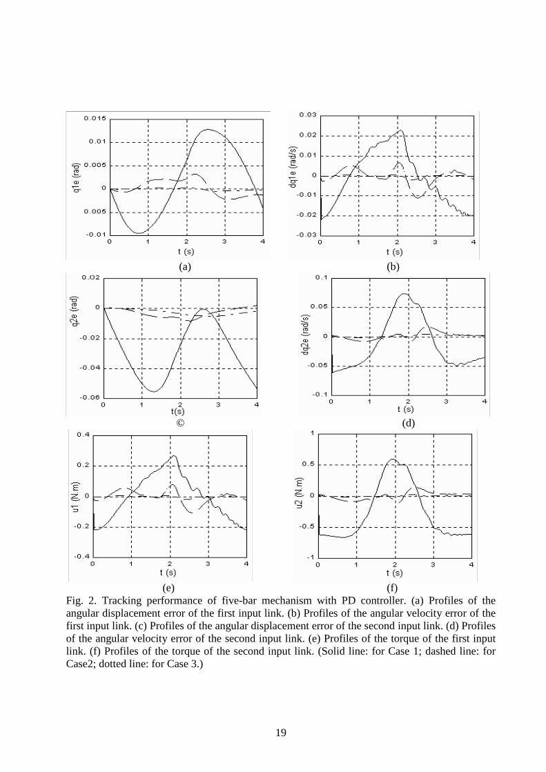
Comparing the simulation results, it is observed that, after the mechanical structure is carefully
designed by applying the DFC method, the motion tracking performance of the mechanism is
improved significantly step by step from Case 1, to Case 2, and to Case 3. Fig. 2 (a) and (c) show
that the angular displacement tracking errors of two input links are largely reduced in Case 2,
and are further reduced in Case 3. Fig. 2 (c) and (d) show that the angular velocity tracking errors
of two input links are largely improved in Case 2, and the better results are obtained in Case 3.
14
From the control torque profiles shown in Fig. 2 (e) and (f), it is indicated that less control
energy is consumed in Case 2 and Case 3.
In a word, the simulation results shown in Fig. 2 reveal that, by applying the DFC method, not
only can the motion tracking performance be improved, but also the control energy is largely cut.
4.2 Analysis of Simulation 2
In this subsection, we compare the original five-bar mechanism with the CTC controller with the
five-bar mechanism with CIPE and PCIGI with the PD controller. The CTC controller is chosen
as follows:
)(),())(( qgqqqCeKeKqqD dp ′+′′+++′= &&&&& dττττ (49)
The PD controller is the same as equation (48). The gain matrices of two controllers are chosen
to be IK p 10= and IK 50=d .
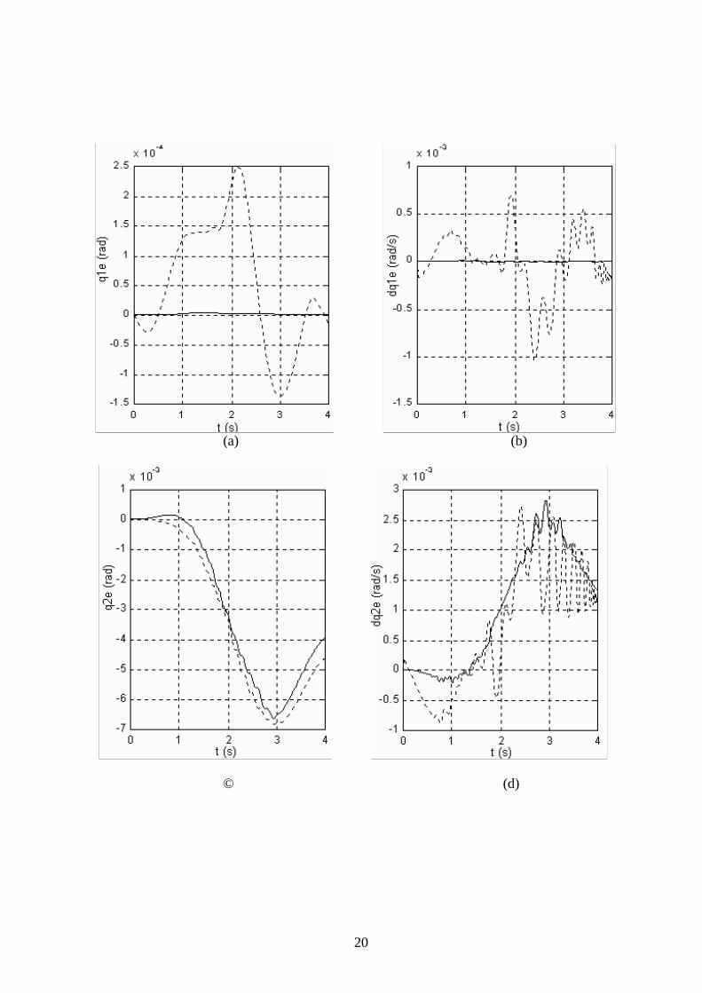
The simulation results are shown in Fig. 3. Fig. 3 (a) and (c) depict profiles of the angular
displacement errors of two input links under the two different cases, which indicate that although
the tracking errors are less in Case 1 with the CTC controller than in Case 3 with the PD
controller, the difference between them is only by 0.00025 (rad). Fig. 3 (b) and (d) depict profiles
of the angular velocity errors of two input links under the two different cases, which indicate
again that although the tracking errors are in less Case 1 with the CTC controller than in Case 3
with the PD controller, the difference between them is only by 0.001 (rad/s). It is interesting to
note that the maximum errors of the second input link in two cases are almost the same. In a
word, Fig. 3 (a)-(d) have shown that the difference of tracking performances of Case 1 with the
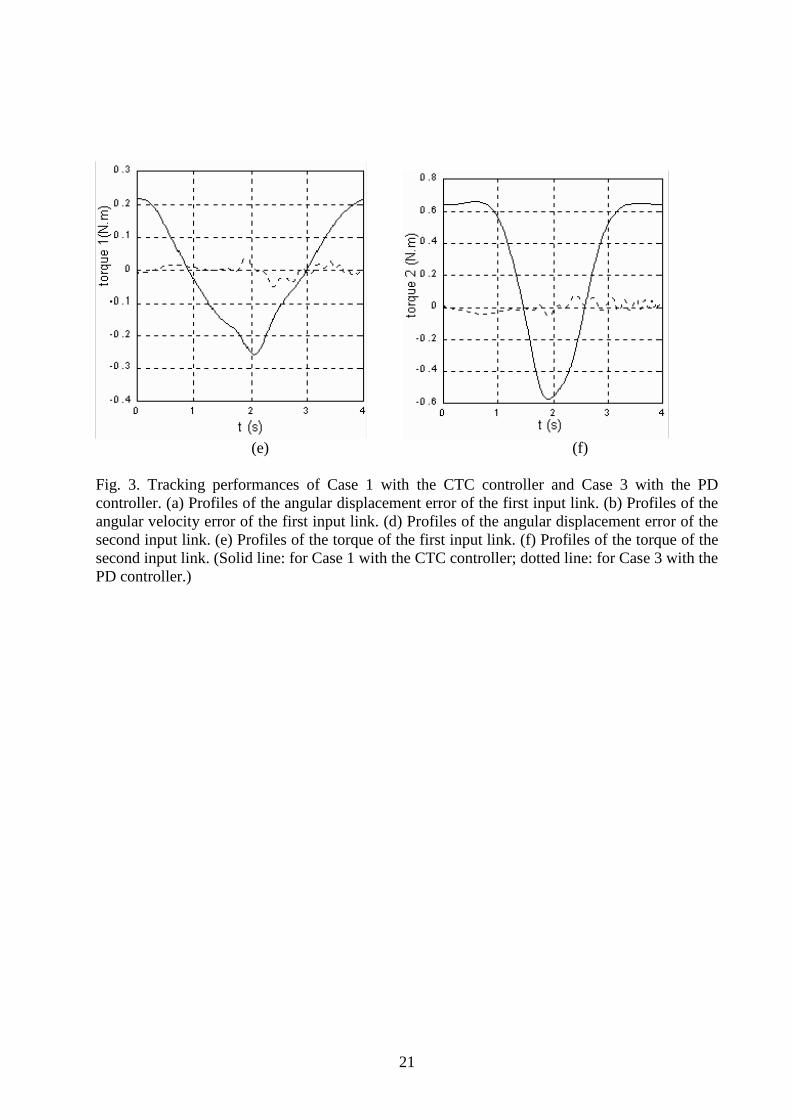
CTC controller and Case 3 with the PD controller is not significant. However, Fig. 3 (e) and (f),
which depict profiles of the torques of the two input links, show that Case 1 with the CTC
controller consumes ten times more control energy than Case 3 with the PD controller.
5. Conclusion
15
It is shown from the preceding discussion that the careful design of the mechanical structure with
the properties such as CIPE, CIGI and PCIGI can significantly facilitate the controller design.
And this can further lead to the improvement of system performance in terms of trajectory
tracking errors and torques in the two servomotors. When the PD controller is applied to the case
without CIPE, CIGI and PCIGI (Case 1), the case with CIPE (Case 2), and the case with both
CIPE and PCIGI (Case 3), the system performance are significantly improved from Case 1, to
Case 2, and to Case 3. The CTC controller applied to Case 1 does not improve the trajectory
tracking performance with respect to Case 3; however, produces about 10 times higher torque in
Case 1 than in Case 3.
Acknowledgement
This research reported in this paper has been partially supported by Natural Sciences and
Engineering Research Council (NSERC) in Canada
References
[1]. D. Stewart, A platform with six degrees of freedom, Proceedings of Institute of Mechani-
cal Engineering, London, U. K., 1966. pt. I, Vol. 108, pp371-386
[2] W. J. Zhang, Q. Li, and L. S. Guo, Integrated design of mechanical structure and control
algorithm for a programmable four-bar-linkage, IEEE/ASME Transaction on
Mechatronics, 1999, 4(4): 345-362.
[3] F. Ghorbel, O. Chetelat, R. Gunawardana, and R. Longchamp, Modeling and set point
control of closed-chain mechanisms: theory and experiment, IEEE Transaction on
Control Systems Technology, 2000, 8(5):801-815.
[4] John J. Craig, Introduction to Robotics: Mechanics and Control, 2nd edition, Addision
Wesley, Readin, Massachussetts, 1989.
[5] Richard M. Murray, Zexiang Li, and S, Shankar Sastry, A mathematical Introduction to
Robotic Manipulator, CRC Press Inc., 1994.
[6] John J. Craig. Adaptive Control of Mechanical Manipulator, Addision-Wesley Publishing
Company. 1988.
16
[7] J. E. Slotine and W. Li, Applied Nonlinear Control, Englewood Cliffs, N.J. : Prentice
Hall, 1991
[8] R. Ortega and M. W. Spong, Adaptive motion control of rigid robots: A Tutorial,
Automatica, 1989, 25(6):877~888
[9] M. C. Lin and J. S. Chen, Experiment toward MARC deign for linkage system,
Mehanatronics, 1996, 6(6): 933~953.
[10] F. Ghorbel, PD control of closed-chain mechanical systems: An experimental study,
Proceedings of the Fifth IFAC Symposium on Robot Control SYROCO’97, Vol.1:79~84,
Nantes, France, 1997.
[11] F. Ghorbel, A validation study of PD control of closed-chain mechanical systems,
Proceedings of the IEEE 36th Conference on Decision and Control San Diego, December,
1997.
[12] C. M. Gosselin, Parallel computational algorithms for the kinematics and dynamics of
planar and spatial parallel manipulators. ASME J. Dynamics System, Measurement and
Control, 1996, 118(1): 22-28.
[13] H. Asada, and K. Youcef-Toumi, Direct-Drive Robots: Theory and Practice, The MIT
Press,1987
[14] K. Youcef-Toumi and A. T. Y. Kuo, High-Speed Trajectory Control of a Direct-Drive
Manipulator, IEEE Trans. On Robotics and Automation, Vol. 9, no. 1, 1993, pp.102-108.
[15] H. Diken, “Trajectory control of mass balanced manipulator” , Mech. Mach. Theory, 1997,
32(3), 313-322.
[16] W.J. Zhang, and Q. Li, Design for Control: a new principle for technical systems
development, 12th International Conference on Engineering Design, August 24-26, 1999,
Munich, Germany.
[17] F. X. Wu, W. J. Zhang, Q. Li, and P. R. Ouyang, Integrated design and PD control of
High Speed Closed-loop Mechanisms, Submitted to ASME J. Dynamics System,
Measurement and Control.
17
Table I
Mechanical parameters of three cases:
Case 1: original mechanical without any mass redistribution;
Case 2: CIPE;
Case3: CIPE and PCIGI
parameters Case 1 Case2 Case3
1L (m) 0.080 0.080 0.080
2L (m) 0.100 0.100 0.100
3L (m) 0.250 0.250 0.250
4L (m) 0.250 0.250 0.250
5L (m) 0.250 0.250 0.250
1r (m) 0.006 0.0120 0.0307
2r (m) 0.028 0.0885 0.0453
3r (m) 0.125 0.1555 0
4r (m) 0.125 0.1555 0
1m (kg) 0.910 1.210 1.510
2m (kg) 0.280 0.880 1.280
3m (kg) 0.380 0.480 0.580
4m (kg) 0.380 0.480 0.580
1J (×10-3 kg.m2) 0.847 1.285 1.583
2J (×10-3 kg.m2) 0.630 0.930 1.231
3J (×10-3 kg.m2) 4.002 4.532 5.195
2J (×10-3 kg.m2) 4.002 4.632 5.195
1σ (rad) 0 π π
2σ (rad) 0 π π
3σ (rad) 0 0 0
4σ (rad) π π 0
5q (rad) 0 0 0
18
Fig.1 Five-Bar Mechanism
19
(a) (b)
© (d)
(e) (f) Fig. 2. Tracking performance of five-bar mechanism with PD controller. (a) Profiles of the angular displacement error of the first input link. (b) Profiles of the angular velocity error of the first input link. (c) Profiles of the angular displacement error of the second input link. (d) Profiles of the angular velocity error of the second input link. (e) Profiles of the torque of the first input link. (f) Profiles of the torque of the second input link. (Solid line: for Case 1; dashed line: for Case2; dotted line: for Case 3.)
20
(a) (b)
© (d)
21
(e) (f) Fig. 3. Tracking performances of Case 1 with the CTC controller and Case 3 with the PD controller. (a) Profiles of the angular displacement error of the first input link. (b) Profiles of the angular velocity error of the first input link. (d) Profiles of the angular displacement error of the second input link. (e) Profiles of the torque of the first input link. (f) Profiles of the torque of the second input link. (Solid line: for Case 1 with the CTC controller; dotted line: for Case 3 with the PD controller.)