PHYSICAL REVIEW E 94, 032106 (2016)

Integrable matrix theory: Level statistics

Jasen A. Scaramazza,1 B. Sriram Shastry,2 and Emil A. Yuzbashyan1

1Center for Materials Theory, Department of Physics and Astronomy, Rutgers University, Piscataway, New Jersey 08854, USA2Physics Department, University of California, Santa Cruz, California 95064, USA

(Received 7 April 2016; revised manuscript received 14 August 2016; published 2 September 2016)

We study level statistics in ensembles of integrable N × N matrices linear in a real parameter x. The matrixH (x) is considered integrable if it has a prescribed number n > 1 of linearly independent commuting partnersHi(x) (integrals of motion) [H (x),H i(x)] = 0, [Hi(x),H j (x)] = 0, for all x. In a recent work [Phys. Rev. E 93,052114 (2016)], we developed a basis-independent construction of H (x) for any n from which we derived theprobability density function, thereby determining how to choose a typical integrable matrix from the ensemble.Here, we find that typical integrable matrices have Poisson statistics in the N → ∞ limit provided n scalesat least as log N ; otherwise, they exhibit level repulsion. Exceptions to the Poisson case occur at isolatedcoupling values x = x0 or when correlations are introduced between typically independent matrix parameters.However, level statistics cross over to Poisson at O(N−0.5) deviations from these exceptions, indicating thatnon-Poissonian statistics characterize only subsets of measure zero in the parameter space. Furthermore, wepresent strong numerical evidence that ensembles of integrable matrices are stationary and ergodic with respectto nearest-neighbor level statistics.

DOI: 10.1103/PhysRevE.94.032106

I. INTRODUCTION

It is generally believed that the energy levels of integrablesystems [1] follow a Poisson distribution [2–8]. For example,the probability that a normalized spacing between adjacentlevels lies between s and s + ds is expected to be P (s)ds =e−sds. In contrast, chaotic systems exhibit Wigner-Dysonstatistics, with level repulsion P (s) ∝ s2 or s at small s.Moreover, level statistics are often used as a litmus testfor quantum integrability even though there are integrablemodels that fail this test, e.g., the reduced BCS model [5](which is a particular linear combination of commuting GaudinHamiltonians). In this work, we quantify when and whyPoisson statistics occur in quantum integrable models, whilealso characterizing exceptional (non-Poisson) behavior.

Poisson statistics have been numerically verified on acase-by-case basis for some quantum integrable systems,including the Hubbard [2] and Heisenberg [2,3] models. Onthe other hand, general or analytic results on the spectraof quantum integrable models are lacking, in part due tothe absence of a generally accepted unambiguous notion ofquantum integrability [9,10], and in part because existingresults usually apply to isolated models instead of membersof statistical ensembles like random matrices [11]. Notably,Berry and Tabor showed [4] that level statistics in semiclassicalintegrable models are always Poissonian as long as theenergy E(n1,n2, . . . ) is not a linear function of the quantumnumbers n1,n2, . . . , i.e., the system cannot be represented as acollection of decoupled harmonic oscillators. As integrabilityis destroyed by perturbing the Hamiltonian, the statistics areexpected to cross over from Poisson to Wigner-Dyson atperturbation strengths as small as the inverse system size [3].

Random matrix theory (RMT) [11,12] captures levelrepulsion and other universal features of eigenvalue statisticsin generic (nonintegrable) Hamiltonians (see, e.g., Fig. 1). Werecently proposed an integrable matrix theory [13] (IMT) todescribe eigenvalue statistics of integrable models. This theoryis based on a rigorous notion of quantum integrability and

provides ensembles of integrable matrix Hamiltonians withany given number of integrals of motion (see below). It issimilar to RMT in that both are ensemble theories equippedwith rotationally invariant probability density functions. Animportant difference is that random matrices do not representrealistic many-body models, while integrable ones correspondto actual integrable Hamiltonians. We therefore have accessnot only to typical features, but also to exceptional casesand are in a position to make definitive statements aboutthe statistics of quantum integrable models. Here, we studythe nearest-neighbor level spacing distributions of the IMTensembles.

The approach of Refs. [10,13–18] to quantum integrabilityoperates with N × N Hermitian matrices linear in a realparameter x. A matrix H (x) = xT + V is called integrable[16,17,19] if it has a commuting partner H (x) = xT + V otherthan a linear combination of itself and the identity matrix andif H (x) and H (x) have no common x-independent symmetry,i.e., no � �= c1 such that [�,H (x)] = [�,H (x)] = 0. Fixingthe parameter dependence makes the existence of commutingpartners a nontrivial condition, so that only a subset of measurezero among all Hermitian matrices of the form xT + V areintegrable [17].

Further, integrable matrices fall into different classes(types) according to the number of independent integrals ofmotion. We say that H (x) is a type-M integrable matrix if thereare precisely n = N − M > 1 linearly independent N × N

Hermitian matrices [20] Hi(x) = xT i + V i with no commonx-independent symmetry such that

[H (x),H i(x)] = 0, [Hi(x),H j (x)] = 0, (1)

for all x and i,j = 1, . . . ,n. A type-M family of integrablematrices (integrable family) is an n-dimensional vector space[20], where Hi(x) provide a basis. The general member of thefamily is

H (x) =n∑

i=1

diHi(x), (2)

2470-0045/2016/94(3)/032106(17) 032106-1 ©2016 American Physical Society

SCARAMAZZA, SHASTRY, AND YUZBASHYAN PHYSICAL REVIEW E 94, 032106 (2016)

FIG. 1. The level spacing distribution of a 4000 × 4000 randomreal symmetric matrix with entries chosen as independent randomnumbers from a normal distribution of mean 0 and off-diagonalvariance 1

2 (diagonal variance of 1). Such a matrix belongs to theGaussian orthogonal ensemble (GOE) of real symmetric matrices,studied in random matrix theory (RMT). The main feature of thespacing distribution here is its vanishing for small spacings, alsoknown as level repulsion. The smooth curve is the Wigner surmiseP (s) = π

2 se− π4 s2

. See the integrable matrix case in Fig. 2.

where di are real numbers. The maximum possible value of n isn = N − 1, corresponding to type-1 or maximally commutingHamiltonians.

Examples of well-known many-body Hamiltonians thatfit into this definition of integrability are the Gaudin, one-dimensional (1D) Hubbard, and XXZ models, where x

corresponds to the external magnetic field, Hubbard U ,and the anisotropy, respectively. Note, however, that thesemodels have various x-independent symmetries, such as thez component of the total spin, total momentum, etc. Takenat a given number of spins or sites, they break down intosectors (matrix blocks) characterized by certain parameter-independent symmetry quantum numbers. Such blocks areintegrable matrices according to our definition. For instance,the 1D Hubbard model on six sites with three spin up and threespin down electrons is a direct sum of integrable matrices ofvarious types [17]. Sectors of Gaudin magnets, where the z

component of the total spin differs by one from its maximumor minimum value (one spin flip) or, equivalently, the oneCooper pair sector of the BCS model are type-1 [16], whileother sectors are integrable matrices of higher types.

Prior work [10,15–18] constructed all type-1, -2, -3 inte-grable matrices and a certain subclass of arbitrary type-M ,determined exact eigenvalues and eigenfunctions of thesematrices, investigated the number of level crossings as afunction of size and type, and showed that type-1 integrablefamilies satisfy the Yang-Baxter equation. This work is acontinuation of Ref. [13] where we formulated a rotationallyinvariant parametrization of integrable matrices and derivedan appropriate probability density function (PDF) for theparameters, i.e., for ensembles of integrable matrices ofany given type. The derivation is similar to that in theRMT and is based on either maximizing the entropy of thePDF or, equivalently, postulating statistical independence of

FIG. 2. The level spacing distribution for a 4000 × 4000 realsymmetric integrable matrix H (x) = xT + V at x = 1. This par-ticular matrix is a sum of 200 linearly independent matrices thatcommute for all values of the real parameter x. Note that the spacingdistribution is maximized at s = 0, a feature known as level clustering.The smooth curve is a Poisson distribution, which is theorized to betypical of integrable matrices. Compare to the generic real symmetricmatrix case in Fig. 1.

independent parameters and rotational invariance of the PDF.Here, we use the results of Ref. [13] to generate and studynumerically and analytically level spacing distributions inensembles of integrable matrices of various types as well as inindividual matrices.

Our main results are as follows. For a generic choice ofparameters, the level statistics of integrable matrices H (x) arePoissonian in the limit of the Hilbert space size N → ∞ ifthe number of conservation laws n scales at least as log N (seeFig. 2 for an example). Exceptions to Poisson statistics fallinto two categories. First, it is always possible to construct anintegrable matrix that has any desired level spacing distributionat a given isolated value x = x0 of the coupling (or externalfield) parameter. For a typical type-1 matrix there is always asingle value of x where the statistics are Wigner-Dyson. Thedistribution quickly crosses back over, however, to Poissonat deviations from x0 of size δx ∼ N−0.5, with the crossovercentered at δx ∼ N−1. Second, one obtains non-Poissoniandistributions by introducing correlations among the ordinarilyindependent parameters characterizing an integrable matrixH (x); the reduced BCS model falls into this category. Thestatistics again revert to Poisson at O(N−0.5) deviations fromsuch correlations. We also show numerically that as N → ∞,integrable matrix ensembles satisfy two distinct definitionsof ergodicity with respect to the nearest-neighbor spacingdistribution P (s). Not only are the statistics of a single matrixrepresentative of the entire ensemble, but the statistics of thej th bulk spacing across the ensemble are independent of j .

In Sec. II, we present numerical results on the level statisticsof type-1 matrices, defined to be integrable matrices H (x) withthe maximum number nmax = N − 1 of linearly independentcommuting partners. Section III contains numerical results forintegrable matrices with n � nmax. We present our analyticaljustification of numerical results using perturbation theory inSec. IV. Finally, we give numerical results on ergodicity inSec. V.

032106-2

INTEGRABLE MATRIX THEORY: LEVEL STATISTICS PHYSICAL REVIEW E 94, 032106 (2016)

II. LEVEL STATISTICS OF TYPE-1INTEGRABLE MATRICES

A. Type-1 families, primary parametrization

Although our definition of integrable matrices encompassesthe general Hermitian case, we restrict our focus in this workto real symmetric matrices. We begin with type-1 integrableN × N families which contain N − 1 nontrivial commutingpartners in addition to the scaled identity (c1x + c2)1. Suchmatrices are the simplest to construct, for the parametrizationof type-M integrable families increases in complexity with M .Results on these higher types are deferred to Sec. III.

We first summarize the essential points of the basis-independent type-1 construction of Ref. [13] in order toarrive at the parametrization of Eq. (4) useful for numericalcalculations. By considering linear combinations of the N − 1basis matrices, defined in Eq. (2), and the identity, one canprove that every type-1 family contains a particular integrablematrix �(x) with rank-1 T part

�(x) = x |γ 〉 〈γ | + E, (3)

i.e., [H (x),�(x)] = 0 for all x and any H (x) = xT + V inthe family. There is an additional restriction [V,E] = 0, whichfollows from O(x0) term in the commutator. It can be shownthat the matrices E and V and the vector |γ 〉 completelydetermine a given type-1 matrix H (x) = xT + V modulo anadditive constant proportional to the scaled identity.

If we consider any type-1 H (x) in the shared eigenbasisof E and V , we find that the matrix elements of H (x) canbe parametrized in terms of the N eigenvalues εi of E, theN eigenvalues di of V , and the N vector components γi of|γ 〉. Statistical arguments borrowed from RMT in Ref. [13]identify the εi and di as two independent sets of eigenvaluesdrawn from the Gaussian orthogonal ensemble. The γi aredrawn from a δ(1 − |γ |2) distribution. With these parameters,any N × N type-1 integrable matrix H (x) = xT + V can beconstructed in the following way:

[H (x)]ij = xγiγj

di − dj

εi − εj

, i �= j

[H (x)]jj = dj − x∑k �=j

γ 2k

dj − dk

εj − εk

. (4)

We call Eq. (4) the “primary” parametrization, which isgiven specifically in the basis where V is diagonal andcan be transformed into any other basis by an orthogonaltransformation. Note that the quantities dj act as coefficients oflinear combination of basis matrices Hi(x) defined by settingdj = δij in Eq. (4). Explicitly, nonzero matrix elements ofHi(x) are

[Hi(x)]ij = [Hi(x)]ji = xγiγj

εi − εj

, j �= i

[Hi(x)]jj = −xγ 2

i

εi − εj

, j �= i

[Hi(x)]ii = 1 − x∑k �=i

γ 2k

εi − εk

, (5)

and

H (x) =N∑

i=1

diHi(x). (6)

From Eq. (6) we see that the εi and γi uniquely identify atype-1 commuting family whereas the choice of di produces agiven member of the family.

To describe the spectrum of H (x), we introduce an addi-tional N parameters λj = λj (x) determined by the followingequation [16]:

1

x=

N∑k=1

γ 2k

λj − εk

. (7)

One can graphically verify that for any nondegenerate choiceof εk there are N real solutions λj to Eq. (7) that interlace theεk . The N eigenvectors v(x) and eigenvalues η(x) of H (x) arelabeled by λj and take the form

[vλj(x)]k = γk

λj − εk

, ηλj(x) = x

N∑i=1

diγ2i

λj − εi

. (8)

The components of the (unnormalized) eigenvectors vλj(x) are

independent of the choice of di in Eq. (6), and are thus commonto any member of the family defined by εk and γk .

B. Universality of Poisson statistics

Equipped with parametrizations of integrable matrix en-sembles based on the number of commuting partners in afamily, we can quantitatively outline both the origin andthe robustness of Poisson statistics in these ensembles. Wefirst explore the latter with numerical tests of the statisticsof integrable matrices in Secs. II C–III C. For clarity ofexposition, the numerical results of Secs. II C, II D, and II E aredemonstrated strictly for type-1 matrices. In Sec. III, we showthat the same results apply generally to a construction of highertype integrable matrix families that by definition contain fewerthan the maximum number of conservation laws. We presentanalytical considerations of numerical results in Sec. IV.

We emphasize that regardless of the choice of parameterswe find Poisson level statistics in the overwhelming majorityof cases, even near isolated points in parameter space withnon-Poissonian statistics. For example, the least biased choicefor di in Sec. II A enforces GOE statistics at x = 0 sinceH (0) = V ; by effecting a shift x → x + x0, the equivalentinvariant statement is that each type-1 matrix has a parametervalue x0 such that H (x0) has Wigner-Dyson statistics. Anotherexception to Poisson statistics is when di and εi are correlatedso that di = f (εi), a smooth function at least over almost theentire range of εi . Nonetheless, as soon as we deviate from x0

or f (εi), the results of Secs. II C and II D show that statisticsquickly revert to Poisson at deviations scaling as δ ∼ N−0.5 inthe limit N → ∞.

Generally, we find that random linear superpositions ofbasis matrices within a given integrable family are crucial forobtaining Poisson level statistics. Basis matrices themselves,defined in Eq. (6) for the primary type-1 construction andin Eq. (22) for more general integrable matrices, shownon-Poissonian statistics with strong level repulsion. Such

032106-3

SCARAMAZZA, SHASTRY, AND YUZBASHYAN PHYSICAL REVIEW E 94, 032106 (2016)

repulsion washes away, however, for H (x) that are randomlinear combinations of sufficiently many basis matrices. Wesee this behavior in Sec. II E for all type-1 matrices, i.e.,independent of the number m of basis matrices (conservationlaws) in linear combination as long as m > O(log N ).

We fit all spacing distributions P (s) to the Brody function[21] P (s,ω), where ω is the Brody parameter

P (s,ω) = a(ω)sωe−b(ω)sω+1. (9)

The distribution in Eq. (9) has unit mean and norm withappropriate choices of constants a(ω) and b(ω). It interpolatesbetween a Poisson distribution P (s) = e−s at ω = 0 and theWigner surmise P (s) = π

2 se− π4 s2

at ω = 1, and hence is aconvenient fitting function. The Brody parameter ω can takeall values ω > −1, which means it also can detect enhancedlevel clustering or repulsion.

Note, however, that the Wigner surmise is not the exactnearest-neighbor spacing distribution of GOE matrices. Onemay therefore expect our numerics to produce an ω �= 1 forGOE matrices. Figure 4, where ω ≈ .956, shows that this isindeed the case. The exact distribution P (s) can be found inRef. [11] and was originally derived by Gaudin in terms of aFredholm determinant [22]. Using Ref. [23] and a few linesof Mathematica code, we find that the same fitting procedureused for numerically generated matrices produces ω ≈ 0.957.Note that it is important to exclude P (0) = 0 in the fittingprocedure for numerically generated finite-sized matrices.

C. Crossover in coupling parameter x

Here, we show that even if the statistics are non-Poissonianat a given coupling value x = x0 (we set x0 = 0), levelclustering is restored at small deviations from x0. For any N ,the matrices T and V each have eigenvalues that mostly lie onan O(1) interval centered about zero. We consider the primarytype-1 construction encountered in Eq. (4) and explore thelevel statistics of large matrices. In Fig. 3, we see qualitativelyhow the statistics change with x when N = 4000. We findPoisson statistics at x ∼ 1 until a crossover to level repulsionbegins near x = N−0.5 and ends near x = N−1.5.

To verify that the crossover scaling inferred from Fig. 3is correct for all N 1, in Fig. 4 we plot how the Brodyparameter ω [see Eq. (9)] evolves with x for various choicesof N . It turns out that ω(x,N ) can be fit to a relatively simplefunction, for any N 1,

ω(x,N ) = α − β tanh

(logN x − X0

Z

). (10)

The numbers (α,β,X0,Z) are fit parameters and take the values(0.482,0.474,−1.04,0.157) in Fig. 4. Most important is thatfor any N 1 we find X0 ∼ −1, which solidifies our claimthat the crossover occurs between x ∼ N−1.5 and x ∼ N−0.5.Analytical arguments explaining this scaling are given inSec. IV.

D. Correlations between matrix parameters

In the eigenbasis of V , our parametrization of integrableN × N matrices is given in terms of about 3N independent

FIG. 3. Crossover in coupling x of the level statistics of type-1 integrable N × N matrices H (x) = xT + V , N = 4000. SeeSec. II A for their parametrization. V is a random matrix so thatH (x = 0) has level repulsion. Each distribution contains the levelsstatistics of a single matrix H (x) at a given value of x. Note that somelevel repulsion has set in by x = N−1. Each numerical distributionis fit to the Brody function P (s,ω) from Eq. (9); for couplingsx = (1,N−1,N−1.5) the fits give ω = (0.01,0.30,0.94), respectively.The solid lines are reference plots of a Poisson distribution P (s) = e−s

and the Wigner surmise P (s) = π

2 se− π4 s2

. See Fig. 4 for more on thiscrossover.

parameters (up to a change of basis). Through an explicitconstruction of the probability density function of integrablematrices obtained through basis-independent considerations,Ref. [13] shows that for a typical integrable matrix, di and εi are

FIG. 4. Crossover in level statistics with variation of couplingparameter x in type-1 integrable N × N matrices H (x) = xT + V ,quantified by the Brody parameter ω(x,N ) from Eq. (9). The twoimportant limits are ω = 0 for Poisson statistics and ω = 1 forrandom matrix (Wigner-Dyson) statistics. Each plotted value ω(x,N )is computed for the combined level spacing distribution of severalmatrices from the ensemble. We extract the crossover scale byfitting ω(x,N ) to Eq. (10) (solid curve) to all curves simultaneously,where most notably X0 ∼ −1 for all N investigated, indicating thatcrossovers to Poisson statistics are centered at that value for integrablematrices H (x) when H (x = 0) has level repulsion. The middle of thecrossover is indicated by a vertical line.

032106-4

INTEGRABLE MATRIX THEORY: LEVEL STATISTICS PHYSICAL REVIEW E 94, 032106 (2016)

FIG. 5. Level statistics of two N × N type-1 integrable matri-ces H (x) = xT + V , x = 1 and N = 4000, when correlations areintroduced between dj and εj [see Eqs. (4), (8), and then Eq. (11)for an example]. Note that in contrast to Fig. 3, these integrablematrices exhibit level repulsion even for x = 1. Each of the twocurves is generated from a single matrix. One numerical curvecorresponds to the case when di = εi and the other is when di =∑4

k=1 Akhk(εi), where hk(z) is the kth order Hermite polynomial and(A1,A2,A3,A4) = (2.3,2.16,−1.46,0.51), chosen randomly. Notethat the polynomial dependence weakens the level repulsion ascompared to the linear case. If higher order polynomials are included,the level repulsion eventually gives way to Poisson statistics. The solidcurve is the Wigner surmise P (s) = π

2 se− π4 s2

. See Fig. 7 for more onthis behavior.

indeed uncorrelated. We see in this section that if correlationsare introduced between εi and di , the statistics becomenon-Poissonian. Small perturbations about these correlations,however, bring the statistics immediately back to Poisson. Inthis section, x = 1 for all matrices considered.

Continuing with type-1 matrices in the primaryparametrization [Eq. (4)] we recall that the eigenvalues ηλj

ofsuch a matrix H (x) = xT + V are given by Eq. (8),where theλj = λj (x) are obtained from Eq. (7). As we saw in Sec. II C,a typical choice of parameters will produce Poisson statistics,but this changes if we let di be some smooth function of εi . Thesimplest case is shown in Fig. 5 for which di = εi . As discussedin Refs. [13,17], H (x) for this choice of parameters describesa sector of the reduced BCS model and, independently, ashort range impurity in a weakly chaotic metallic quantumdot studied in Refs. [24,25].

The level repulsion for this case can be understood by asimple manipulation of Eq. (8) when di = εi :

ηλj= x

N∑i=1

εiγ2i + λjγ

2i − λjγ

2i

λj − εi

= −x

N∑i=1

γ 2i + λj ,

(11)

where we used Eq. (7). Then, when di = εi the eigenvaluesof H (x) are just the λj up to an additive constant. For thecase when εi are random matrix eigenvalues, Ref. [24] derivesthe joint probability density of the set {εi,λj } and Ref. [25]demonstrates that the λj are subject to the same level repulsion

FIG. 6. Illustrating that conclusions drawn about correlations be-tween di (eigenvalues of V ) and εi (eigenvalues of E) are independentof the particular choice of εi . Pictured are four numerically generatednearest-neighbor spacing distributions P (s) for 5000 × 5000 type-1matrices, x = 1, when the di and εi are either from a random matrix(GOE) or are independently and identically distributed numbers(i.i.d.) from a normal distribution. Each curve represents the levelstatistics of a single matrix chosen from the type-1 ensemble. Levelrepulsion survives in the two cases where di and εi are correlated(V = E), even though the overall shape of P (s) depends on whetherE’s eigenvalues are GOE or i.i.d. numbers. The solid curves arethe usual Poisson distribution P (s) = e−s and the Wigner surmiseP (s) = π

2 se− π4 s2

. We do not include plots for different choices of γi ,which do not affect the general character of the results.

as the εi . Note also that Eq. (7) implies λj lie betweenconsecutive εi and therefore the eigenvalues in Eq. (11) canhave no crossings at any finite x. Numerically, we have foundthat λj exhibit level repulsion for any choice of εi (seeFig. 6). Figure 5 also shows the level repulsion induced whendi = ∑4

k=1 Akhk(εi), where hk(εi) is the kth order Hermitepolynomial and Ak are independent random numbers drawnfrom a normal distribution. In this case, the level repulsionis mitigated relative to the case of linear correlation. Sums tohigher orders of hk(εi) (or any higher order polynomial) willeventually bring the statistics back to Poisson.

We now investigate the stability of induced level repulsionin H (x) when correlations between di and εi are broken.In Fig. 7, we let di = εi(1 + δDi) where Di is an O(1)random number from a normal distribution and δ is a numbercontrolling the size of the perturbation. The crossover toPoisson statistics as δ increases is very similar to that in Fig. 4,which shows the crossover with x. In fact, we can fit the Brodyparameter ω(δ,N ) to

ω(δ,N ) = α − β tanh

(logN δ − X0

Z

). (12)

Note that Eq. (12) is just Eq. (10) with the substitution x → δ.We find that the crossover occurs over the range N−1.5 � δ �N−0.5, indicating that any perturbation to correlations willimmediately destroy level repulsion as N → ∞. In partic-ular, Fig. 7 gives (α,β,X0,Z) = (0.479,0.474,−1.03,0.169)for linear correlations. This scaling is not restricted tothe case di = εi , as seen in Fig. 8 where we again

032106-5

SCARAMAZZA, SHASTRY, AND YUZBASHYAN PHYSICAL REVIEW E 94, 032106 (2016)

FIG. 7. Variation in the Brody parameter ω(δ,N ) when di =εi(1 + δDi) in the level statistics of N × N type-1 integrable matricesH (x) for various N , x = 1. The number δ is a parameter controllingthe size of the perturbation from correlation, and Di is an O(1) randomnumber from a normal distribution. Note that the crossover in δ is verysimilar to that in x shown in Fig. 4. The numerical curves are fit tothe function ω(δ,N ) given in Eq. (12) (solid curve), with a crossovercentered at X0 ∼ −1, indicating that crossovers to Poisson statisticsare centered at that value. Each plotted value ω(δ,N ) is computed forthe combined level spacing distribution of several matrices from theensemble. A vertical line indicates the center of the crossover on theplot. For a similar plot for nonlinear functions di(εi), see Fig. 8.

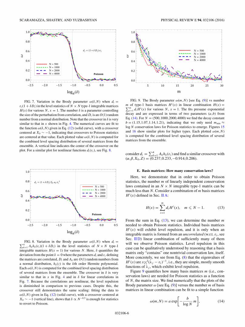
FIG. 8. Variation in the Brody parameter ω(δ,N ) when di =∑4k=1 Akhk(εi)(1 + δDi) in the level statistics of N × N type-1

integrable matrices H (x = 1) for various N . Here, δ quantifies thedeviation from the point δ = 0 where the parameters di and εi definingthe matrices are correlated, Di and Ak are O(1) random numbers froma normal distribution, hk(z) is the kth order Hermite polynomial.Each ω(δ,N ) is computed for the combined level spacing distributionof several matrices from the ensemble. The crossover in δ is verysimilar to that in x in Fig. 4 and in δ for linear correlations inFig. 7. Because the correlations are nonlinear, the level repulsionis diminished in comparison to previous cases. Despite this, thecrossover still demonstrates the same scaling: fitting the data toω(δ,N ) given in Eq. (12) (solid curve), with a crossover centered atX0 ∼ −1 (vertical line), shows that δ ∝ N−0.5 is enough for statisticsto revert to Poisson.

FIG. 9. The Brody parameter ω(m,N ) [see Eq. (9)] vs numberm of type-1 basis matrices Hi(x) in linear combination H (x) =∑m

i=1 diHi(x) for various N , x = 1. The fits presume exponential

decay and are expressed in terms of two parameters (a,b) fromEq. (14). For N = (500,1000,2000,4000) we find the decay constantb = (1.15,1.07,1.14,1.21), indicating that we only need mmin ≈log N conservation laws for Poisson statistics to emerge. Figures 15and 16 show similar plots for higher types. Each plotted ω(m,N )is computed for the combined level spacing distribution of severalmatrices from the ensemble.

consider di = ∑4k=1 Akhk(εi) and find a similar crossover with

(α,β,X0,Z) = (0.237,0.233,−0.914,0.206).

E. Basis matrices: How many conservation laws?

Here, we demonstrate that in order to obtain Poissonstatistics, the number m of linearly independent conservationlaws contained in an N × N integrable type-1 matrix can bemuch less than N . Consider a combination of m basis matricesHi(x) defined in Sec. II A:

H (x) =m∑

i=1

diHi(x), m � N − 1. (13)

From the sum in Eq. (13), we can determine the number m

needed to obtain Poisson statistics. Individual basis matricesHi(x) will exhibit level repulsion, and it is only when anintegrable matrix is formed from an uncorrelated (w.r.t. εi , seeSec. II D) linear combination of sufficiently many of themwill we observe Poisson statistics. Level repulsion in thiscase can be qualitatively understood by reasoning that a basismatrix only “contains” one nontrivial conservation law, itself.More concretely, we see from Eq. (8) that the eigenvalues ofHi(x) are xγ 2

i (λj − εi)−1, i.e., they are simple, mostly smoothfunctions of λj , which exhibit level repulsion.

Figure 9 quantifies how many basis matrices m (i.e., con-servation laws) are needed for Poisson statistics as a functionof N , the matrix size. We find numerically that the plots of theBrody parameter ω [see Eq. (9)] versus the number m of basismatrices in linear combination can be fit to a simple function

ω(m,N ) = a exp

[− b

log Nm

], (14)

032106-6

INTEGRABLE MATRIX THEORY: LEVEL STATISTICS PHYSICAL REVIEW E 94, 032106 (2016)

where a and b are real constants. The fact that for differentvalues of N we find that b ∼ 1 supports the notion that weneed only about log N conservation laws in order to inducePoisson statistics. We make this claim with caution becausewe only have data for 500 � N � 4000, a range over whichlog N does not vary significantly. More precisely, Fig. 9 showsthat having m = O(1) conservation laws is insufficient forinducing Poisson statistics, and that a useful upper bound onthe lowest m necessary for Poisson statistics is mmin < O(Nα)where 0 < α < 0.20. We obtain the factor of 0.20 byrewriting Eq. (14) assuming the decay constant has power lawdependence on N instead of logarithmic dependence

ω(m,N ) = a exp[− c

Nαm

]. (15)

Numerically, we found that the parameter b in Eq. (14)satisifies 1.07 � b � 1.21 when 500 � N � 4000. Bymatching exponents between Eqs. (15) and (14) for(b1,N1) = (1.21,500) and (b2,N2) = (1.07,4000), we find amaximum exponent α = 0.198.

The basis matrices Hi(x) contained in any integrable H (x)are linearly independent conservation laws. The observeddependence of P (s) on the number m of basis matricesin linear combination is reminiscent of the early work ofRosenzweig and Porter [26] (RP) on the nearest-neighborspacing distribution of superpositions of independent spectra.Although the spectra of basis matrices Hi(x) are not strictlyindependent and are added together instead of superposed(“superposed” here means “combined into a single list”), wesee the same qualitative behavior as described by RP: a singlebasis matrix has level repulsion, but a sufficiently large numbercombined have Poisson statistics. In the case of m independent,superposed spectra with vanishing P (0) that contribute equallyto the mean level density, the value Pm(0) of the superposedspectrum is given by the RP result

Pm(0) = 1 − 1

m. (16)

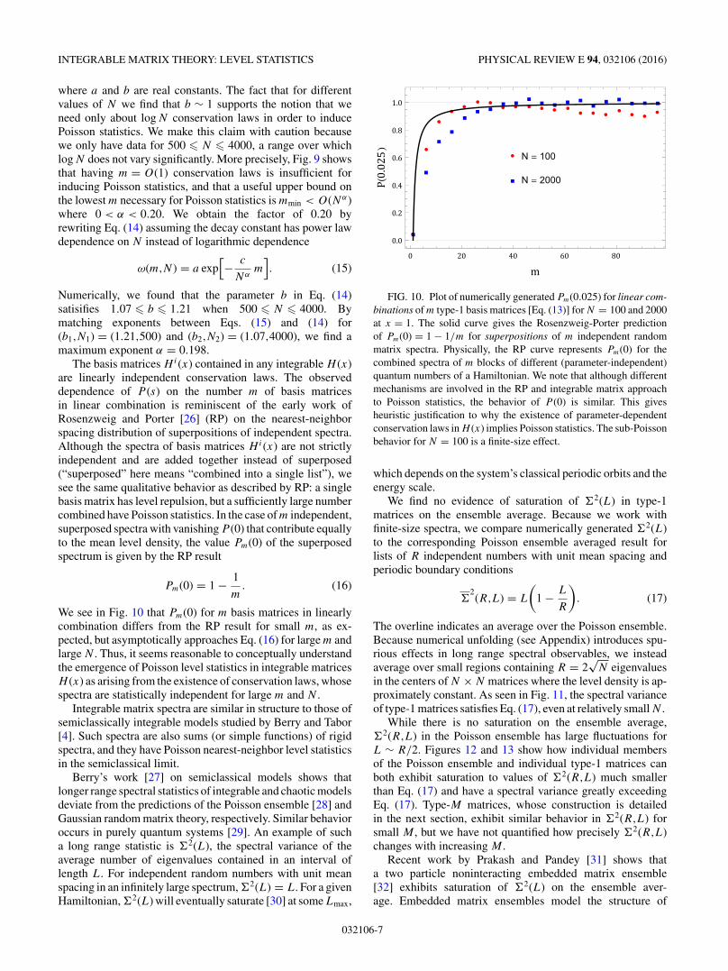
We see in Fig. 10 that Pm(0) for m basis matrices in linearlycombination differs from the RP result for small m, as ex-pected, but asymptotically approaches Eq. (16) for large m andlarge N . Thus, it seems reasonable to conceptually understandthe emergence of Poisson level statistics in integrable matricesH (x) as arising from the existence of conservation laws, whosespectra are statistically independent for large m and N .

Integrable matrix spectra are similar in structure to those ofsemiclassically integrable models studied by Berry and Tabor[4]. Such spectra are also sums (or simple functions) of rigidspectra, and they have Poisson nearest-neighbor level statisticsin the semiclassical limit.

Berry’s work [27] on semiclassical models shows thatlonger range spectral statistics of integrable and chaotic modelsdeviate from the predictions of the Poisson ensemble [28] andGaussian random matrix theory, respectively. Similar behavioroccurs in purely quantum systems [29]. An example of sucha long range statistic is 2(L), the spectral variance of theaverage number of eigenvalues contained in an interval oflength L. For independent random numbers with unit meanspacing in an infinitely large spectrum, 2(L) = L. For a givenHamiltonian, 2(L) will eventually saturate [30] at some Lmax,

FIG. 10. Plot of numerically generated Pm(0.025) for linear com-binations of m type-1 basis matrices [Eq. (13)] for N = 100 and 2000at x = 1. The solid curve gives the Rosenzweig-Porter predictionof Pm(0) = 1 − 1/m for superpositions of m independent randommatrix spectra. Physically, the RP curve represents Pm(0) for thecombined spectra of m blocks of different (parameter-independent)quantum numbers of a Hamiltonian. We note that although differentmechanisms are involved in the RP and integrable matrix approachto Poisson statistics, the behavior of P (0) is similar. This givesheuristic justification to why the existence of parameter-dependentconservation laws in H (x) implies Poisson statistics. The sub-Poissonbehavior for N = 100 is a finite-size effect.

which depends on the system’s classical periodic orbits and theenergy scale.

We find no evidence of saturation of 2(L) in type-1matrices on the ensemble average. Because we work withfinite-size spectra, we compare numerically generated 2(L)to the corresponding Poisson ensemble averaged result forlists of R independent numbers with unit mean spacing andperiodic boundary conditions

2(R,L) = L

(1 − L

R

). (17)

The overline indicates an average over the Poisson ensemble.Because numerical unfolding (see Appendix) introduces spu-rious effects in long range spectral observables, we insteadaverage over small regions containing R = 2

√N eigenvalues

in the centers of N × N matrices where the level density is ap-proximately constant. As seen in Fig. 11, the spectral varianceof type-1 matrices satisfies Eq. (17), even at relatively small N .

While there is no saturation on the ensemble average, 2(R,L) in the Poisson ensemble has large fluctuations forL ∼ R/2. Figures 12 and 13 show how individual membersof the Poisson ensemble and individual type-1 matrices canboth exhibit saturation to values of 2(R,L) much smallerthan Eq. (17) and have a spectral variance greatly exceedingEq. (17). Type-M matrices, whose construction is detailedin the next section, exhibit similar behavior in 2(R,L) forsmall M , but we have not quantified how precisely 2(R,L)changes with increasing M .

Recent work by Prakash and Pandey [31] shows thata two particle noninteracting embedded matrix ensemble[32] exhibits saturation of 2(L) on the ensemble aver-age. Embedded matrix ensembles model the structure of

032106-7

SCARAMAZZA, SHASTRY, AND YUZBASHYAN PHYSICAL REVIEW E 94, 032106 (2016)

FIG. 11. Ensemble averaged number variance 2(R,L) in N ×

N type-1 matrices H (x) = xT + V at x = 1 for N = 100 and 1000.In order to achieve a constant mean level spacing normalized tounity, we selected the middle R = 2

√N eigenvalues from each matrix

and used periodic boundary conditions on the list of eigenvalues.The results are in excellent agreement with the Poisson ensemblepredictions (solid curves), given by Eq. (17). There is no saturationon the ensemble average. We averaged over 104 matrices for N = 100and 500 matrices for N = 1000.

many-body systems by constructing eigenenergies out ofrandom k-body interactions between m particles k < m.Reference [31] contains an extended discussion of saturationand helpful references. We do not pursue spectral variancefurther in this work.

III. STATISTICS OF INTEGRABLE MATRICESOF HIGHER TYPES

A. Ansatz type-M families

We do not yet have a method for directly generalizing thetype-1 primary parametrization from Sec. II A to higher type

FIG. 12. Deviations from the Poisson ensemble average Eq. (17)

(solid curve) of number variance 2(200,L) from two members of the

Poisson ensemble. Shown are the number variances of two differentlists of 200 independent numbers from a flat distribution in orderto illustrate the large fluctuations of long-range spectral observablesin the Poisson ensemble. See Fig. 13 for similar behavior in type-1spectra.

FIG. 13. Deviations from the Poisson ensemble average Eq. (17)

(solid curve) of number variance 2(64,L) from two members of

the N = 1000 type-1 ensemble. Shown are the number variances oftwo matrices used in the ensemble average of Fig. 11. The saturationobserved in the more rigid of the two spectra is reminiscent of thatseen in members of the Poisson ensemble (see Fig. 12).

matrices that by definition have fewer commuting partners.Instead, we present another parametrization that producesa subset of integrable families of any type M � 1. Theconstruction is in terms of 3N + 1 real parameters so that inchoosing values for them one obtains a matrix H (x) = xT +V with a desired number n of nontrivial commuting partners(n = N − M) and no parameter-independent symmetries. Asin the type-1 primary parametrization, the parameters can betraced back to eigenvalues of two commuting constant randommatrices and a random vector.

Here, we present the results; more details can be found inRef. [17] while the rotationally invariant construction is givenin Ref. [13]. Again in the diagonal basis of V , the most generalmember of an ansatz type-M commuting family is

[H (x)]ij = xγiγj

(di − dj

εi − εj

)�i + �j

2, i �= j

(18)

[H (x)]ii = di − x∑j �=i

γ 2j

(di − dj

εi − εj

)1

2

(�i + �j )(�j + 1)

�i + 1,

where

〈i|i〉 ≡N∑

j=1

γ 2j

(λi − εj )2,

di = 1

x0

N−M∑j=1

gj

〈j |j〉1

λj − εi

, (19)

�i = ±√√√√1 + 1

x0

N∑j=N−M+1

Pj

〈j |j〉1

λj − εi

.

This parametrization gives all type-1, -2, and -3 integrablematrices and only a subset of such for higher types. Wecall matrices obtained by this construction ansatz type M asopposed to all type M , these two notions being equivalent forM = 1,2,3.

032106-8

INTEGRABLE MATRIX THEORY: LEVEL STATISTICS PHYSICAL REVIEW E 94, 032106 (2016)

Basis-independent considerations from Ref. [13] identify λi

as eigenvalues of a matrix � selected from the GOE and γi asselected from a δ(1 − |γ |2) distribution, as was the case for theprimary parametrization of type-1 matrices in Sec. II A. Onemay alternatively select the εi as eigenvalues of a GOE matrixE and from them derive the λi . We find that this choice has noeffect on the statistics. Unique to the ansatz parametrization arethe (N − M) parameters gi and M parameters Pi . Reference[13] identifies these parameters as eigenvalues selected froman N × N GOE matrix G [33] satisfying [G,�] = 0. The signof �i can be chosen arbitrarily for each i and each set of signchoices corresponds to a different commuting family. The λi

by construction are solutions of the following equation witharbitrary (but fixed) real x0 �= 0:

f (λi) ≡N∑

j=1

γ 2j

λi − εj

− 1

x0= 0,

F (εi) ≡N∑

j=1

1

〈j |j 〉1

λj − εi

− x0 = 0.

(20)

The second line of Eq. (20) follows from the first by writingboth the partial fraction decomposition and factorized formof F (z) = 1/f (z) and matching residues. Equations (19) and(20) mean that ansatz type-M matrices are written in terms ofan auxiliary primary type-1 problem with parameter x0 and(unnormalized) eigenstates |i〉 [see Eq. (7) and Ref. [13]].Note the important distinction between x and x0, namely, thatx is free but x0 is fixed for a given family of commutingmatrices.

Due to the square root in the expression for �i [Eq. (19)],a given set of Pi will typically result in a complex set of �i .The matrix H (x) will subsequently be complex symmetric,rather than real, although it will still satisfy all requirements ofintegrability. Because in this work we study the eigenvalues ofreal symmetric integrable matrices, we elect to reparametrize�i in a way that guarantees they be real without awkwardlyscaling each set of Pi :

�i = ±√√√√∏N

j=1(φj − εi)∏Nk=1(λk − εi)

, (21)

where the M φj are real parameters such that (upon orderingεj and λj for argument’s sake) εj < φj < λj if x0 > 0 andλj < φj < εj if x0 < 0. The resulting �i are real valued. Asthere is no existing basis-independent interpretation for φj ,we simply choose them from a uniform distribution on theirallowed intervals. We find that the choice of φi or Pi to generatethe �j has a numerically undetectable effect on the eigenvaluestatistics.

Varying parameters gj produces different matrices withinthe same commuting family, while varying the remainingparameters γi,λi,φi,x0 generate sets of matrices from differentfamilies. A natural way to choose a basis for the ansatz type-Mcommuting family is to define the n = N − M nontrivialHk(x) such that gj = δkj in Eq. (19) for 1 � j � N − M .

In other words,

Hk(x) = xT k + V k is given by Eq. (18) with

di → dki = 1

x0

1

〈k|k〉1

λk − εi

(22)

for k = 1, . . . ,N − M . In particular,

V k = Diag(dk

1 ,dk2 , . . . ,dk

N

). (23)

A general member of the commuting family is

H (x) =N−M∑k=1

gkHk(x) (24)

up to a multiple of the identity trivial to the study of levelspacing statistics.

Ansatz type-M families have an exact solution in terms of asingle equation similar to Eq. (7) given in Ref. [17], which hasslight differences in notation as compared to here. To studylevel statistics of ansatz matrices, we numerically diagonalizethem rather than use the computationally cumbersome exactsolution.

A fundamental difference between ansatz type-M matricesand the primary type-1 parametrization is that the eigenvaluesof the matrix V in the former are heavily constrained byEq. (19), while in the latter they are free parameters. Inparticular, as explained in Ref. [13] the primary type-1 V isselected from the GOE, while the ansatz V is a certain primarytype-1 matrix evaluated at x = −x0, i.e.,

V (x0) = −x0TH1 + H1, (25)

where H1 has N − M arbitrary eigenvalues gi and M eigenval-ues equal to zero. By the results of Sec. II, ansatz V = V (x0)will typically have Poisson statistics. The resolution to thisapparent disconnect between the two parametrizations is thatfor |x0| 1, V (x0) will have the eigenvalue statistics of H1.We argue in Ref. [13] that the N − M gi are a subset ofeigenvalues of an N × N matrix from the GOE, so that for M

not too large and x0 1 we obtain Wigner-Dyson statistics inansatz V .

We then forgo studying crossovers in the coupling x of levelstatistics of ansatz type-M matrices H (x) = xT + V becauseansatz V have Poisson statistics for typical parameter choices.Instead, we focus on the behavior of the statistics with respectto parameter correlations, the number M , and the number ofbasis matrices. In all numerical work on ansatz matrices weset x0 = 1, as this is a typical coupling value for the auxiliarytype-1 problem.

B. Correlations in ansatz parameters

Building on the results of Sec. II D, here we explore effectsof parameter correlations on the statistics in general type-Mansatz matrices. Introducing correlations between di and εi inthis case is more complicated than in Sec. II D because thedi here are not all independent. Fortunately, Eq. (19) admitsa simple way to produce such correlations. As an example,

032106-9

SCARAMAZZA, SHASTRY, AND YUZBASHYAN PHYSICAL REVIEW E 94, 032106 (2016)

FIG. 14. Variation in the Brody parameter ω(δ,N ) when gi =λi(1 + δGi) in the level statistics of N × N ansatz type-M integrablematrices H (x = 1) [Eq. (18)] for various N and M . Ordered pairs inthe legend indicate size and type (N,M) of the matrices, δ controls thestrength of the perturbation from the point δ = 0 where the parametersgi and λi defining these integrable matrices are correlated, and Gi isan O(1) random number from a normal distribution. The crossoverin δ for small M is similar to the primary type-1 crossovers in δ

and x seen in Figs. 4, 7, and 8. For larger M , correlations cannot beintroduced by this method [see Eq. (26)]. Despite type-M matriceshaving fewer than the maximum number of conservation laws, thecrossover still demonstrates the scaling given in Eq. (12) (solid curves)with a crossover centered around X0 ∼ −1 (vertical line). As before,deviations from correlation of size δ ∝ N−0.5 are enough for thestatistics to become Poisson. Each plotted value ω(δ,N ) is computedfor the combined level spacing distribution of several matrices fromthe ensemble. For the case of correlations in ansatz matrices, wechoose all �k > 0 in order to avoid pathological statistics in H (x).

consider the case when gj = λj :

di = 1

x0

N−M∑j=1

λj − εi + εi

〈j |j〉1

λj − εi

= 1

x0εi

⎛⎝N−M∑

j=1

1

〈j |j〉1

λj − εi

⎞⎠ + (const)

= εi

⎛⎝1 − 1

x0

M∑j=1

1

〈j |j〉1

λj − εi

⎞⎠ + (const),

(26)

where the second part of Eq. (20) was used. The sums in thethird line of Eq. (26) introduce a randomizing factor that hasa weak effect for small M but that destroys the correlationbetween di and εi at intermediate values of M . Figure 14shows the now familiar level statistics crossover in δ for ansatzmatrices of different size and type with gk = λk(1 + δGk),where Gk is an O(1) random number chosen from a normaldistribution and δ a parameter controlling the size of theperturbation. Just as in Sec. II D, the crossover to Poissonstatistics is centered about δ ∼ N−1. More generally, we caninduce level repulsion in ansatz type-M matrices if M N

when gk = f (λk), a smooth function of λk .

5 10 15 20

0.0

0.2

0.4

0.6

0.8

M = 497M = 480M = 250

FIG. 15. Graph of the Brody parameter ω(m,N ) given by Eq. (9)vs number m of ansatz type-M basis matrices Hk(x) [see Eq. (22)]contained in linear combination H (x) = ∑m

k=1 gkHk(x) for N = 500,

x = 1. The fits presume exponential decay and are expressed in termsof two parameters (a,b) from Eq. (14). For M = (250,480) we find thedecay constant b = (1.13,1.04), indicating that we only need mmin ≈log N conservation laws for Poisson statistics to emerge, independentof type. We do not observe Poisson statistics for M = 497 because themaximum number of nontrivial basis matrices is 3 in this case, and wesee that we need at least ∼15 conservation laws for Poisson statisticsto start emerging for N = 500. See Fig. 16 for a similar plot forN = 2000 and Fig. 9 for the same concept in type-1 matrices. Eachplotted value ω(m,N ) is computed for the combined level spacingdistribution of several matrices from the ensemble.

C. Basis matrices: Ansatz higher types

We now generalize the type-1 results of Sec. II E to apply toall ansatz type-M matrices. Recall that a general ansatz type-Mmatrix H (x) = xT + V can be written as a linear combinationof basis matrices Hk(x) for which gi = δik [see Eq. (24)].

We see again in Figs. 15 and 16 that Poisson statisticsemerge for relatively small linear combinations of basismatrices. Denoting m as the number of conservation lawscontained in a linear combination, i.e.,

H (x) =m∑

i=1

gkHk(x), m � N − M (27)

we investigate the Brody parameter ω(m,N ) from Eq. (14).In Fig. 15, N = 500, ω(m,N ) decays to zero as a functionof m in nearly the same way for M = 470 as for M = 20.It is only for very large M , such as M = 497, that levelclustering is forbidden, and this only because we can use amaximum of three nontrivial basis matrices. Similar behavioremerges for N = 2000 in Fig. 16. For all N and M testedwe find b ∼ 1 (with precise values given in the captions).Therefore, we can estimate a similar bound as in Sec. II E forthe minimum number of conservation laws needed for Poissonlevel statistics, namely, mmin < O(Nα) where 0 < α < 0.25,obtained from the M = N/2 cases. Since m cannot exceedthe total number of conservation laws n = N − M for type-Mmatrices, this provides a lower bound nmin = mmin < O(Nα)consistent with mmin ≈ log N .

032106-10

INTEGRABLE MATRIX THEORY: LEVEL STATISTICS PHYSICAL REVIEW E 94, 032106 (2016)

FIG. 16. Brody parameter ω(m,N ) [see Eq. (9)] vs number m

of ansatz type-M basis matrices Hk(x) [see Eq. (22)] containedin linear combination H (x) = ∑m

k=1 gkHk(x) for N = 2000, x = 1.

The fits presume exponential decay and are expressed in terms of twoparameters (a,b) from Eq. (14). For M = (1000,1980) we find thedecay constant b = (0.99,1.03), indicating that we only need mmin ≈log N conservation laws for Poisson statistics to emerge, independentof type. We do not observe Poisson statistics for M = 1997 becausethe maximum number of nontrivial basis matrices is 3 in this case,and we see that we need at least ∼20 conservation laws for Poissonstatistics to start emerging for N = 2000. See Fig. 15 for a similar plotfor N = 500 and Fig. 9 for the same concept in type-1 matrices. Eachplotted value ω(m,N ) is computed for the combined level spacingdistribution of several matrices from the ensemble.

IV. ANALYTICAL RESULTS: PERTURBATION THEORY

Some of the numerical observations found in Secs. IIand III can be understood using perturbation theory in theparameter x. We restrict our analysis to the primary type-1parametrization because our arguments for this case are muchmore transparent than for the ansatz construction. The analysisfor ansatz matrices is similar.

The eigenvalues ηm(x) of H (x) to first order in x are givenby the second equation in Eq. (4), where we set constant|γj |2 = N−1 for clarity and to achieve proper scaling for largeN :

ηm(x) ≈ dm − x

N

∑j �=m

(dm − dj

εm − εj

). (28)

The first term comes from V , which has a Wigner-DysonP (s), and the second term from T , which is determined bythe integrability condition and whose level statistics we donot control. Let us estimate the x at which the two terms inEq. (28) become comparable. Note that dk and εk both lie onO(1) intervals so that T and V scale in the same way for largeN . Suppose εk are ordered as ε1 < ε2 < . . . < εN . When dk

and εk are uncorrelated dm − dj is O(1) when j is close to m,i.e., when (εm − εj ) = O(N−1). The second term in Eq. (28)is then xcm ln N , where cm = O(1) is a random number onlyweakly correlated with dm. We performed simple numericaltests that confirm this scaling argument.

If we now order dm, cm in general will not be ordered, i.e.,if dm+1 > dm is the closest level to dm and therefore (dm+1 −dm) = O(N−1), the corresponding difference (cm+1 − cm) =

O(1). The contributions to level spacings from the two termsin Eq. (28) become comparable for x = xc ≈ 1/(N ln N ). Itmakes sense that the second term introduces a trend towardsa Poisson distribution because it is a (nonlinear) superpositionof εk and dk , eigenvalues of two uncorrelated random matrices.Thus, we expect a crossover from Wigner-Dyson to Poissonstatistics near x = xc. In our numerics, we observe a crossoverover the range N−1.5 � x � N−0.5 centered about xc ∼ N−1

likely because we do not reach large enough N to detect thelog component of the crossover.

This argument breaks down when dk = f (εk) since in thiscase (dm − dj ) = O(N−1) when (εm − εj ) = O(N−1). Thetwo terms in Eq. (28) become comparable only at x = O(1);moreover, the second term no longer trends towards Poissonstatistics. Relaxing the correlation between dk and εk withdk = f (εk)(1 + δDk), Dk = O(1), and going through thesame argument, one expects a crossover to Poisson statisticsat δ = O(1/N ln N ) when x = O(1).

The level repulsion observed in basis matrices is a conse-quence of the level repulsion implicit in the parameters λi ,independent of the choice of εi [see the text below Eq. (11)and Fig. 6]. Indeed, basis matrices Hi(x) in the primary type-1parametrization (4) have eigenvalues ηi

j (x) = xγ 2i (λj − εi)−1,

which is a smooth function of λj except near εi . The ηij (x)

therefore inherit the level repulsion of the λj . Analogousreasoning applies to ansatz basis matrices.

V. ERGODICITY IN INTEGRABLE MATRIX ENSEMBLES

The discussion and figures in this section make frequentreference to the “primary” construction of type-1 integrablematrices and the “ansatz” construction of type-M integrablematrices. These parametrizations are introduced in Secs. II Aand III A, respectively. Ensemble averages are taken withrespect to the probability distributions for integrable matricesintroduced in Ref. [13].

One of the goals of this work is to determine the extentto which ensembles of integrable matrices are “ergodic.”Intuitively, an ensemble is called ergodic if a single randomlyselected member has properties that are typical of the entireensemble. Bohigas and Gianonni [34] expound the subject ingenerality for random matrices, and here we focus numericallyon the meaning of ergodicity with regards to the nearest-neighbor level spacing distribution of integrable matrices.Rigorous results on ergodicty for Gaussian ensembles and thePoisson ensemble were derived by Pandey [35].

We distinguish between three separate ways of gener-ating nearest-neighbor eigenvalue spacing distributions forN × N integrable matrix ensembles. We call Pi,N,R(s) thelevel spacing distribution, normalized to unity, of the ithmember of the ensemble obtained from a spectral region R

containing many eigenvalues (infinitely many as N → ∞).The normalized distribution of spacings in R from all matricesin the ensemble is called PN,R(s). A third way to characterizespacing statistics is through the normalized distribution of thej th eigenvalue spacing of all matrices in the ensemble, whichwe call pN,j (s). Both the regions R and the numbers j arestipulated to be far from the edges of the spectrum. In general,Pi,N,R(s), PN,R(s), and pN,j (s) are distinct distributions.Conceptually, PN,R(s) and pN,j (s) are ensemble properties

032106-11

SCARAMAZZA, SHASTRY, AND YUZBASHYAN PHYSICAL REVIEW E 94, 032106 (2016)

FIG. 17. Demonstrating the stationary property (29) in type-1N × N matrices H (x), x = 1 in the primary parametrization. Thefour numerical curves show the statistics pN,j (s) for (N,j ) = (10,3),(10,5), (80,10), and (80,40), each containing 105 eigenvalue spacings.The statistics are nearly independent of j for N = 10, and for N = 80there is no perceptible difference between j = 10 and 40. The solidline is a Poisson distribution p(s) = e−s . Stationarity is shown to holdalso for type-M ansatz matrices in Fig. 18.

while Pi,N,R(s) characterizes the spectrum of an individualmatrix. In the following definitions, we assume that the spacingdistributions converge to a well-defined limit as N → ∞,unlike known pathological examples such as the semiclassicalspacing distribution of a harmonic chain [4]. This assumptionis supported numerically.

We now describe a precise notion [35] of ergodicity thatcharacterizes the limiting behavior of Pi,N,R(s), PN,R(s), andpN,j (s) as N → ∞. First, we must determine whether pN,j (s)is asymptotically stationary, i.e., independent of j :

limN→∞

pN,j (s) = p(s). (29)

In the case of type-1 matrices in the primary parametrization,we see in Fig. 17 that the graphs of two different p10,j (s)closely resemble those of two different p80,j (s), the latter ofwhich are clearly Poisson. The same is true for ansatz matricesof any type, but the convergence to a Poisson distribution doesnot become apparent until N = 300 as in Fig. 18. We concludethat Eq. (29) is true for integrable matrices.

We now turn to the notion of spectral averaging, i.e., thefunction Pi,N,R(s). If Eq. (29) holds, the ensemble averagedPi,N,R(s), called PN,R(s), satisfies

limN→∞

PN,R(s) = p(s), (30)

independent of the region R. In practice, we numericallyunfold the spectrum (see Appendix) in order to take intoaccount any effects a nonstationary mean level spacing canhave on Pi,N,R(s), which characterizes fluctuations about themean level spacing. In this work, we say integrable matricesare spectrally stationary if

limN→∞

Pi,N,R(s) = Pi(s), (31)

and ergodic with respect to nearest-neighbor level statistics if

Pi(s) = p(s). (32)

FIG. 18. Demonstrating the stationarity property (29) in ansatztype-150 N × N matrices H (x), x = 1 and N = 300. The twonumerical curves show the statistics pN,j (s) for (N,j ) = (300,150)and (300,20), each containing ∼104 eigenvalue spacings. Thestatistics are nearly independent of j , although higher N would beneeded in order for the differences to disappear. The solid line is aPoisson distribution p(s) = e−s .

Two points are to be made about Eqs. (31) and (32). First,Eq. (31) is similar in spirit to, but not implied by, Eq. (29).Figures 19–22 show for various integrable matrices, basismatrices included, that the level statistics from a single largematrix Pi,N,R(s) do not depend on the spectral region R used.

Second, the limiting distribution is independent of the indexi, which means that a single matrix’s spacing distributionis typical of the ensemble. In rigorous work on Gaussianensembles [35], this is proved by showing the ensemble

FIG. 19. Demonstrating spectral stationarity [Eq. (31)] in type-1matrices. Shown are the level statistics Pi,N,R(s) of a single (ithmember of the ensemble) type-1 integrable matrix H (x), x = 1and N = 20000, for different regions R of its spectrum containing4000 eigenvalues each. The inset shows the density of states of thismatrix and indicates which numerical curve corresponds to whichregion R. The distributions Pi,N,R(s) shown are independent of R,indicating that type-1 matrix spectra are stationary with respect tonearest-neighbor level statistics. Noting that these distributions arePoisson, Pi,N,R(s) ≈ e−s (solid curve), and comparing to Fig. 23which gives PN ′,R(s) ≈ e−s for N ′ = 2000, we see that ergodicity[Eq. (32)] is satisfied for type-1 integrable matrices.

032106-12

INTEGRABLE MATRIX THEORY: LEVEL STATISTICS PHYSICAL REVIEW E 94, 032106 (2016)

FIG. 20. Level statistics Pi,N,R(s) of a single integrable matrixH (x), x = 1, N = 20 000, and M = 10 000, for different regions R

of its spectrum [the subscript i indicates H (x) is the ith matrix inthe ensemble] containing 4000 eigenvalues each. Inset: the density ofstates of H (x) showing the correspondence between the distributionsand regions R. The distributions Pi,N,R(s) are independent of R,indicating that type-M matrix spectra are stationary with respectto nearest-neighbor level statistics, i.e., Eq. (31) holds. Notingthat these distributions are Poisson, Pi,N,R(s) ≈ e−s (solid curve),and comparing to Fig. 24 which gives PN ′,R(s) ≈ e−s for N ′ =2000, M ′ = 1000, we verify the ergodic property (32).

averaged variance of Pi,N,R(s) vanishes as N → ∞. In thiswork, we compare numerically generated graphs of spectralspacing distributions to ensemble averaged ones for large N .By comparing Figs. 23 and 24 to Figs. 19 and 20, we see that,for large N , Pi,N,R(s) → p(s).

FIG. 21. Demonstrating spectral stationarity [Eq. (31)] in levelstatistics of primary type-1 basis matrices (defined in Sec. II A).Shown are the level statistics Pi,N,R(s) of a single type-1 integrablebasis matrix, x = 1 and N = 20 000, for different regions R of itsspectrum [the subscript i indicates H (x) is the ith matrix in theensemble]. Each spectral region R contains 4000 eigenvalues. Theinset shows the density of states of this matrix and indicates whichnumerical curve corresponds to which region R. The distributionsPi,N,R(s) shown are independent of R, indicating that type-1 basismatrix spectra are stationary with respect to level statistics. Eventhough there is a band gap, the level statistics on either side of the gapare the same. The solid curve is the Wigner surmise P (s) = π

2 se− π4 s2

.

FIG. 22. Demonstrating spectral stationarity [Eq. (31)] in levelstatistics of ansatz basis matrices (defined in Sec. III A). Shown arethe level statistics Pi,N,R(s) of a single type-10 000 integrable ansatzbasis matrix, x = 1 and N = 20 000, for different regions R of itsspectrum [the subscript i indicates H (x) is the ith matrix in theensemble]. The inset shows the density of states of this matrix andindicates which numerical curve corresponds to which region R.The distributions Pi,N,R(s) shown are independent of R, indicatingthat type-M basis matrix spectra are stationary with respect to levelstatistics. Even though there is a band gap, the level statistics on eitherside of the gap are the same. The solid curve is the Wigner surmiseP (s) = π

2 se− π4 s2

. Regions I–III use 4000 eigenvalues apiece, whileregion IV uses only 3000 and gets to within 1% of the spectrum’sedge.

The properties of stationarity and ergodicity are useful ifthey set in quickly for small N because smaller matricesare more accessible both analytically and computationally.A classic example in Gaussian random matrix theory is theWigner surmise, derived from 2 × 2 matrices (see Fig. 1),which is extremely useful for characterizing p(s) in the GOE.

FIG. 23. Demonstrating ergodicity [Eq. (32)] in type-1 matrices(continuing from Fig. 19). A plot of lnPN,R(s), N = 2000 for 100type-1 matrices in the primary parametrization. We do not specifythe spectral region R because Fig. 19 shows that the statistics areindependent of R. The solid line is f (s) = −s, indicating thatPN,R(s)is indeed Poisson for N = 2000 type-1 matrices.

032106-13

SCARAMAZZA, SHASTRY, AND YUZBASHYAN PHYSICAL REVIEW E 94, 032106 (2016)

FIG. 24. Demonstrating ergodicity [Eq. (32)] in type-M ansatzmatrices (continuing from Fig. 20). A plot of lnPN,R(s), N = 2000for 100 type M = 1000 matrices in the ansatz parametrization. Wedo not specify the spectral region R because Fig. 20 shows that thestatistics are independent of R. The solid line is f (s) = −s, indicatingthat PN,R(s) is indeed Poisson for N = 2000 type-1000 matrices.Inset: log-log plot of the same data.

We have seen that the nearest-neighbor level statistics ofintegrable matrices H (x) are generally stationary and ergodic,but the property does not set in for small N as quickly as itdoes for Gaussian random matrices. As an example, Figs. 25and 26 show p3,2(s), the distribution of the second eigenvaluespacing for N = 3, M = 1. This distribution differs markedlyfrom a Poisson distribution, especially in the small s and larges regions. For small s, there is slight level repulsion and forlarge s, Fig. 26 shows that the decay of p3,2(s) is a powerlaw. Numerical data generated in Secs. II and III used bothPi,N,R(s) and PN,R(s) to represent level statistics of integrablematrices. The results of this section show that for large N , itis valid to treat these two distinct distributions as equal.

FIG. 25. Plot of the statistics p3,2(s), the second spacing of 106

type-1 integrable matrices H (x) of size N = 3 with x = 1. Thedistribution is not Poisson (solid line) and actually has a power lawtail (see Fig. 26 for more on the tail). In order to observe the limitp(s) of type-1 integrable matrices, defined in Eq. (29), we need to goto larger N as in Fig. 17.

FIG. 26. Log-log plot of the tail of the distribution p3,2(s) shownin Fig. 25, the statistics of the second spacing of 106 primary type-1 integrable matrices H (x) of size N = 3 with x = 1. The linearfit f (z) = −3.15z + 0.02 shows that this portion of the tail of thedistribution p3,2(s) follows a power law s−α with exponent α ≈ 3.15.Because the distribution pN,j (s) transitions to Poisson for large N ,as evidenced by Fig. 17 for type-1 primary matrices and Fig. 18 fortype-M ansatz matrices, we conclude that exponential behavior in thefar tail of pN,j (s) likely emerges only in the limit N → ∞.

VI. CONCLUSION

Just as ensemble averages in ordinary RMT are used topredict the average behavior of generic quantum systems, therenow exists an analogous ensemble theory- integrable matrixtheory, which we have used to firmly establish the sourceof Poisson statistics and exceptions in quantum integrablemodels.

The goal of this work was to demonstrate two properties ofensembles of type-M integrable N × N matrices linear in acoupling parameter H (x) = xT + V as N → ∞:

(1) The nearest-neighbor spacing distribution P (s) isPoisson, P (s) = e−s , for generic choices of parameters foralmost all M . There are cases of level repulsion, but theycorrespond to sets of measure zero in parameter space.

(2) Integrable matrix ensembles are both stationary andergodic with respect to nearest-neighbor level statistics asdefined in Sec. V. It remains to show whether this ergodicityextends to longer range spectral statistics, such as the numbervariance 2(L).

We find that integrable N × N matrices H (x) have Poissonstatistics as long as the number of conservation laws exceedsnmin ≈ log N (or at most nmin < N0.25). Basis-independentconsiderations require (for type-1) GOE statistics at a fixedx0, but we find that Poisson statistics return at deviationsδx ∼ N−0.5. Correlations between otherwise independentparameters also induce level repulsion, but Poisson statisticsagain return at O(N−0.5) deviations from such correlations.In both cases, the crossover occurs roughly over the rangeN−1.5 � δ � N−0.5.

Some parameter choices produce matrices that correspondto sectors of certain known quantum integrable models,although general parameter choices do not map to knownmodels. Most important is that, in addition to the linearity

032106-14

INTEGRABLE MATRIX THEORY: LEVEL STATISTICS PHYSICAL REVIEW E 94, 032106 (2016)

in x condition, the ensembles of matrices studied in this workare only constrained by symmetry requirements just like theGaussian random matrix ensembles. The only difference hereis that in the integrable case there are many more symmetries,and they are parameter dependent. We therefore expect ourresults to apply generally to quantum integrable models withcoupling parameters.

Although we justified the numerical results to a certaindegree using perturbation theory, an analytic justificationfor Poisson statistics for integrable matrices is still lacking.Given the relatively simple construction of integrable matricesthrough basis-independent relations (i.e., matrix equations)involving familiar RMT quantities such as GOE matrices andrandom vectors [13], we surmise that an analytic demonstra-tion of our numerical results might be feasible, especially inthe type-1 case [see, e.g., the discussion below Eq. (11) andRefs. [24,25]].

It is interesting to note that many-body localized [36](MBL) systems are also expected to display Poisson levelstatistics [37,38], and there exist random matrix ensembleswhich model localization and its statistical signatures [39,40].Such ensembles are basis dependent, which is natural becauselocalization is a basis-dependent property. The commutationrequirements of integrable systems, however, are basis in-dependent, and therefore so is the accompanying integrablematrix theory. A priori, many-body localization and inte-grability are two independent concepts [41]. Despite thisfact, integrable matrices do exhibit a parameter-dependentlocalization property [43] in which almost all eigenstates of thematrix H (x) = xT + V are localized in the basis of V for allvalues of x. The stability of this property when a random matrixperturbation is added to H (x), including the possibility of amultifractal phase accompanying the localized and delocalizedregimes [40], is the subject of future study.

ACKNOWLEDGMENTS

This work was supported in part by the David and LucillePackard Foundation and by the National Science Foundationunder Grant No. NSF PHY11-25915. E.A.Y. also thanks theUniversity of California at Santa Cruz and Kavli Institutefor Theoretical Physics, where a significant part of thisresearch was conducted, for hospitality. The work at UCSCwas supported by the U. S. Department of Energy (DOE),Office of Science, Basic Energy Sciences (BES) under AwardNo. DE-FG02-06ER46319. We acknowledge D. Hansen’scontribution at an early stage of this work, especially to theunfolding technique in Appendix. We also thank J. Lebowitzfor helpful discussions. Finally, we thank the PRE referees forsuggestions and questions that led to a considerably improveddraft of this work.

APPENDIX: UNFOLDING SPECTRA

The eigenvalue spacing distributions P (s), P(s), and p(s)(see Sec. V for definitions) considered in the level statisticsdata in this work characterize the fluctuations of spacingsabout their local means. Unfortunately, a nonconstant densityof states renders the actual spacings inadequate for measuringthese fluctuations. Unfolding the spectrum of a matrix refers

to the replacement of the actual eigenvalues ηj with a newset of numbers with unit mean spacing, but that preserve thecharacter of local fluctuations.

We employ a simple method that essentially approximatesthe inverse density of states (i.e., mean level spacing) of agiven matrix through linear interpolations. First, we writethe eigenvalues ηj in increasing order, and express the j theigenvalue ηj in terms of the actual spacings Sk:

ηj = η1 +j−1∑k=0

Sk. (A1)

No unfolding has taken place as of yet, i.e., this is an exactexpression. Now, we postulate that we can write the kth spacingSk as the product of a smoothly varying local mean spacing sk

and an O(1) fluctuating number ρk = 1 + δk:

ηj = η1 +j−1∑k=0

sk(1 + δk) = η1 +j−1∑k=0

skρk. (A2)

Note that the ρk have the form of fluctuating numbers withunit mean; they will therefore serve as our unfolded spacings.By their definition we can write them as

ρk = ηk+1 − ηk

sk

. (A3)

Therefore, if we calculate the smoothly varying mean levelspacings sk from the given data, we can easily find the unfoldedspacings. The ambiguity in our particular unfolding procedurelies in the calculation of sk because its definition involveschoosing how many spacings over which to average, a quantitywe call 2r:

sk = ηk+r − ηk−r

2r. (A4)

It is important to realize that sk is just the inverse of the densityof states. The parameter r is arbitrary except that it must satisfytwo conditions:

(1) r must be large enough to contain many eigenvalues,which is necessary in order for sk to be a smooth function of k.

(2) r cannot be too large or else sk will actually smoothover features in the true inverse density of states.

In practice, we have chosen r to be the floor function of thesquare root of the maximum number of eigenvalue spacings ν

taken from each matrix. To avoid edge effects we have selectedν = 0.8N . Then, r = �√0.8N�. Here are some typical valuesof r used in this paper:

N = 500, r = 22,

N = 1000, r = 31,

N = 2000, r = 44. (A5)

Such a choice of r grows with N but also is small comparedwith N . In other words, we satisfy the requirement 1 r N

as N → ∞.For even the best choices of r , our unfolding method can

still fail if the inverse density of states varies too quickly orhas singularities. Such a situation arises, for example, in smalllinear combinations of basis matrices [defined in Eqs. (6) and(24)] for any type. Consider, for example, the insets of Figs. 21and 22 that show the densities of state of integrable basis

032106-15

SCARAMAZZA, SHASTRY, AND YUZBASHYAN PHYSICAL REVIEW E 94, 032106 (2016)

matrices. The large portions of the spectra where the density ofstates D(η) drops to zero is typical of small linear combinationsof basis matrices. This behavior is generic for basis matricesof all types, and it can be understood by first considering theexpression for the eigenvalues of a type-1 basis matrix (in theprimary parametrization) where dk = δk,q :

ηj = γ 2q

λj − εq

. (A6)

As both the λj and εj have finite support, ηj in this case willonly approach within a finite distance of zero.

An analogous argument exists for basis matrices in theansatz parametrization for any type. For linear combinationsof a small number of basis matrices, such gaps may overlap,but a mean level spacing sk will still be ill-defined in manyparts of the spectrum. As the number of basis matrices in thelinear combination increases, the gaps smooth out until sk iswell defined everywhere.

Given such gaps in spectra, no choice of r will give theconsistent level statistics. This can be seen numerically byvarying r and observing that P (s) is strongly dependent on r .We must then avoid regions of the spectrum where 1/D(η) ispoorly behaved.

The difficulty in this task is to automate it so that we canunfold many matrices in succession without having to examineeach one by hand. Our solution is to notice that if there area small number of spacings in the spectrum that are manytimes the local mean spacing, the standard deviation of theset of actual spacings will be large. If the standard deviation(normalized by the mean) of the actual spacings is near unity,we can be sure that there are no huge jumps such as the onesin Figs. 21 and 22.

With these considerations, here is our unfolding algorithm:

(i) Calculate SD = standard deviation

meanof the middle

(80% + 2r) of the spectrum’s actual spacings. If SD < 1.2,unfold this region of the spectrum with r = �√0.8N� andcontinue to next matrix. If not, continue to step (ii).

(ii)) Shift the region of the spectrum in question to the rightby 10 eigenvalues.

(iii) If ηmax > η0.9N , use 10 fewer spacings AND restartηmin = η0.1N

(iv) Calculate SD. If SD > 1.2, repeat back to step (ii).If SD < 1.2, unfold this region of the spectrum with r =�√0.8N� and continue to next matrix.

This procedure allows for fewer than 0.8N of the spacingsto be used, but we are guaranteed to only investigate regionsof the spectrum where the mean level spacing accuratelyrepresents the size of a typical spacing. Once a sufficientlylarge number of basis matrices are used in linear combination,the entire middle 80% of the spectrum behaves smoothly andthe procedure given above terminates at step (i) for each matrix.The choice of a maximum SD of 1.2 is somewhat arbitrary,and in some parts of this work we used 1.5 in order to increasecomputation speed (i.e., keep more eigenvalue spacings permatrix). Apart from slight differences in distributions, ourresults are unaffected by this arbitrariness.

The unfolding procedure used in this paper assumes thatthe level statistics are the same in all regions of the spectrum,excluding the edges. Although in principle a Hermitian matrixcan have different spectral statistics in different parts of itsspectrum, we numerically showed in Sec. V that the statisticsare the same in all parts of the spectrum of integrable matricesH (u), i.e., they are translationally invariant.

[1] In this Introduction, by quantum integrable systems, models, orHamiltonians we mean exactly solvable many-body models alsocolloquially called integrable. On the other hand, an “integrablematrix” is a precise concept defined in the fourth and fifthparagraphs.

[2] D. Poilblanc, T. Ziman, J. Bellissard, F. Mila, and G. Montam-baux, Europhys. Lett. 22, 537 (1993).

[3] D. A. Rabson, B. N. Narozhny, and A. J. Millis, Phys. Rev. B69, 054403 (2004).

[4] M. V. Berry and M. Tabor, Proc. R. Soc. London, Ser. A 356,375 (1977).

[5] A. Relano, J. Dukelsky, J. M. G. Gomez, and J. Retamosa, Phys.Rev. E 70, 026208 (2004).

[6] H.-J. Stockmann and J. Stein, Phys. Rev. Lett. 64, 2215(1990).

[7] C. Ellegaard, T. Guhr, K. Lindemann, H. Q. Lorensen, J. Nygard,and M. Oxborrow, Phys. Rev. Lett. 75, 1546 (1995).

[8] R. Puttner, B. Gremaud, D. Delande, M. Domke, M. Martins,A. S. Schlachter, and G. Kaindl, Phys. Rev. Lett. 86, 3747 (2001).

[9] J.-S. Caux and J. Mossel, J. Stat. Mech. (2011) P02023.[10] E. A. Yuzbashyan and B. S. Shastry, J. Stat. Phys. 150, 704

(2013).[11] M. L. Mehta, Random Matrices (Academic, San Diego, 1991).

[12] T. Guhr, A. Muller-Groeling, and H. A. Weidenmuller, Phys.Rep. 299, 189 (1998).

[13] E. A. Yuzbashyan, B. S. Shastry, and J. A. Scaramazza, Phys.Rev. E 93, 052114 (2016).

[14] E. A. Yuzbashyan, B. L. Altshuler, and B. S. Shastry, J. Phys.A: Math. Gen. 35, 7525 (2002).

[15] B. S. Shastry, J. Phys. A: Math. Gen. 38, L431 (2005).[16] H. K. Owusu, K. Wagh, and E. A. Yuzbashyan, J. Phys. A: Math.

Theor. 42, 035206 (2009).[17] H. K. Owusu and E. A. Yuzbashyan, J. Phys. A: math. Theor.

44, 395302 (2011).[18] B. S. Shastry, J. Phys. A: Math. Theor. 44, 052001 (2011).[19] One can equivalently attach the parameter to the V part, i.e.,

write H (u) = T + uV as in some of the previous work, orintroduce two parameters H (x,u) = xT + uV (see Ref. [13])for more detail.

[20] Two matrices are considered equal if they differ by a multipleof the identity (c1x + c2)1, which is not included in Hi(x).For example, linear independence means that

∑i aiH

i(x) =(c1x + c2)1 iff ai = 0.

[21] T. A. Brody, Lett. Nuovo Cimento 7, 482 (1973).[22] M. Gaudin, Nucl. Phys. 25, 447 (1961).[23] F. Bornemann, Math. Comput. 79, 871 (2010).

032106-16

INTEGRABLE MATRIX THEORY: LEVEL STATISTICS PHYSICAL REVIEW E 94, 032106 (2016)

[24] I. L. Aleiner and K. A. Matveev, Phys. Rev. Lett. 80, 814 (1998).[25] E. Bogomolny, P. Leboeuf, and C. Schmit, Phys. Rev. Lett. 85,

2486 (2000).[26] N. Rosenzweig and C. E. Porter, Phys. Rev. 120, 1698 (1960).[27] M. V. Berry, Proc. R. Soc. London, Ser. A 400, 229 (1985).[28] Any ensemble composed of lists of independent random

numbers is referred to as the “Poisson” ensemble.[29] T. H. Seligman, J. J. M. Verbaarschot, and M. R. Zirnbauer,

J. Phys. A: Math. Gen. 18, 2751 (1985).[30] Berry works with the spectral ridigity, which is a statistic closely

related to the number variance.[31] R. Prakash and A. Pandey, Phys. Rev. E 93, 052225 (2016).[32] T. A. Brody, J. Flores, J. B. French, P. A. Mello, A. Pandey, and

S. S. M. Wong, Rev. Mod. Phys. 53, 385 (1981).[33] In this work, the gj indeed are eigenvalues from an N × N

GOE matrix, but are selected as a set of N − M consecutiveeigenvalues instead of N − M randomly chosen ones. Thischoice does not affect the level statistics.

[34] O. Bohigas and M. J. Giannoni, Ann. Phys. (NY) 89, 393 (1975).[35] A. Pandey, Ann. Phys. (NY) 119, 170 (1979).[36] D. M. Basko, I. L. Aleiner, and B. L. Altshuler, Ann. Phys. (NY)

321, 1126 (2006).[37] V. Oganesyan and D. A. Huse, Phys. Rev. B 75, 155111

(2007).[38] A. Pal and D. A. Huse, Phys. Rev. B 82, 174411 (2010).[39] P. Shukla, Phys. Rev. E 71, 026226 (2005).[40] V. E. Kravtsov, I. M. Khaymovich, E. Cuevas, and M. Amini,

New J. Phys. 17, 122002 (2015).[41] MBL seems to be a broader class. Even though certain integrals

of motion have been identified in MBL systems (see Ref. [42]for example), they have not been shown to be exactly solvableor integrable as defined in this paper.

[42] M. Serbyn, Z. Papic, and D. A. Abanin, Phys. Rev. Lett. 111,127201 (2013).

[43] R. Modak, S. Mukerjee, E. A. Yuzbashyan, and B. S. Shastry,New J. Phys. 18, 033010 (2016).

032106-17