Embed Size (px)
Citation preview
Integer Multicommodity Flows in Optical
Networks
Diplomarbeit
vorgelegt von
Matthias A.F. Peinhardt
Marz 2003
Technische Universitat Berlin
Fakultat 2 – Mathematik und Naturwissenschaften
Institut fur Mathematik
Studiengang Technomathematik
Erstgutachter: Prof. Dr. M. GrotschelZweitgutachter: Prof. Dr. R. Mohring

2

Acknowledgements
This work has not been possible without the help of many people, I am greatly thankful.
I am grateful to my supervisor Prof. Martin Grotschel, who taught me what mathematicsis about.
I’d like to thank my advisers Dr. Arie Koster and Adrian Zymolka for their support andproof-reading, and their (sometimes challenging) comments. All people at the Konrad-Zuse-Zentrum deserve credit for being addressees of my questions.
All that would not be possible without the (not only material) support I received from theStudienstiftung des deutschen Volkes.
Special thanks to E.N. and Sophie-Charlotte for cheering me up in long nights of typing.
I thank my family, who has always been an anchor throughout my life, and no words couldexpress what I owe them.
Finally, my gratitude goes to Hannah for supporting me in many ways, in any aspect oflife. Without this it all would not have been worth it...
i

ii
Contents
1 Introduction 1
1.1 Notation and preliminaries . . . . . . . . . . . . . . . . . . . . . . . . . . . 2
2 Problem description 5
2.1 Background of the problem . . . . . . . . . . . . . . . . . . . . . . . . . . . 5
2.1.1 Optical networks . . . . . . . . . . . . . . . . . . . . . . . . . . . . . 5
2.1.2 Optical network design . . . . . . . . . . . . . . . . . . . . . . . . . . 7
2.2 Specification . . . . . . . . . . . . . . . . . . . . . . . . . . . . . . . . . . . . 9
2.3 Variations of the problem . . . . . . . . . . . . . . . . . . . . . . . . . . . . 10
2.4 Related work . . . . . . . . . . . . . . . . . . . . . . . . . . . . . . . . . . . 12
2.4.1 Complexity . . . . . . . . . . . . . . . . . . . . . . . . . . . . . . . . 13
2.4.2 Theoretical results . . . . . . . . . . . . . . . . . . . . . . . . . . . . 13
2.4.3 Research on approximation . . . . . . . . . . . . . . . . . . . . . . . 16
2.4.4 Research on solution methods . . . . . . . . . . . . . . . . . . . . . . 16
3 Model and formulations 19
3.1 Model . . . . . . . . . . . . . . . . . . . . . . . . . . . . . . . . . . . . . . . 19
3.2 Formulations . . . . . . . . . . . . . . . . . . . . . . . . . . . . . . . . . . . 21
3.2.1 Edge-flow based formulation . . . . . . . . . . . . . . . . . . . . . . . 21
3.2.2 Path-flow based formulation . . . . . . . . . . . . . . . . . . . . . . . 23
3.2.3 Resource-directed formulation . . . . . . . . . . . . . . . . . . . . . . 24
3.2.4 Convex cost formulation . . . . . . . . . . . . . . . . . . . . . . . . . 25
3.3 Polyhedral investigation . . . . . . . . . . . . . . . . . . . . . . . . . . . . . 27
4 Subgradient method 31
4.1 Theoretical framework . . . . . . . . . . . . . . . . . . . . . . . . . . . . . . 31
iii
iv CONTENTS
4.1.1 General scheme . . . . . . . . . . . . . . . . . . . . . . . . . . . . . . 32
4.1.2 Constrained programs . . . . . . . . . . . . . . . . . . . . . . . . . . 35
4.2 Application to IMCF-N . . . . . . . . . . . . . . . . . . . . . . . . . . . . . 39
4.2.1 Step length selection . . . . . . . . . . . . . . . . . . . . . . . . . . . 42
4.2.2 Projection method . . . . . . . . . . . . . . . . . . . . . . . . . . . . 43
4.2.3 Penalty functions . . . . . . . . . . . . . . . . . . . . . . . . . . . . . 47
4.2.4 Barrier functions . . . . . . . . . . . . . . . . . . . . . . . . . . . . . 47
4.2.5 Using barrier-penalty functions . . . . . . . . . . . . . . . . . . . . . 47
4.2.6 Exact penalty approach . . . . . . . . . . . . . . . . . . . . . . . . . 48
4.2.7 Obtaining integral solutions . . . . . . . . . . . . . . . . . . . . . . . 49
5 Branch-and-cut method 53
5.1 Theoretical framework . . . . . . . . . . . . . . . . . . . . . . . . . . . . . . 53
5.1.1 Cutting plane method . . . . . . . . . . . . . . . . . . . . . . . . . . 53
5.1.2 Branch-and-bound . . . . . . . . . . . . . . . . . . . . . . . . . . . . 55
5.1.3 Branch-and-cut . . . . . . . . . . . . . . . . . . . . . . . . . . . . . . 58
5.2 Application to IMCF-N . . . . . . . . . . . . . . . . . . . . . . . . . . . . . 59
5.2.1 Branching rule . . . . . . . . . . . . . . . . . . . . . . . . . . . . . . 59
5.2.2 Node selection . . . . . . . . . . . . . . . . . . . . . . . . . . . . . . 60
5.2.3 Heuristics . . . . . . . . . . . . . . . . . . . . . . . . . . . . . . . . . 60
5.2.4 Cutting planes . . . . . . . . . . . . . . . . . . . . . . . . . . . . . . 60
6 Computational results 63
6.1 Implementation . . . . . . . . . . . . . . . . . . . . . . . . . . . . . . . . . . 63
6.2 Test instances . . . . . . . . . . . . . . . . . . . . . . . . . . . . . . . . . . . 63
6.3 Results . . . . . . . . . . . . . . . . . . . . . . . . . . . . . . . . . . . . . . . 65
6.3.1 Results of the subgradient method . . . . . . . . . . . . . . . . . . . 65
6.3.2 Results of the branch-and-cut method . . . . . . . . . . . . . . . . . 67
6.3.3 Comparison of the results . . . . . . . . . . . . . . . . . . . . . . . . 68
7 Conclusions 69
7.1 Evaluation of the subgradient approach . . . . . . . . . . . . . . . . . . . . 69
7.2 Evaluation of the branch-and-cut approach . . . . . . . . . . . . . . . . . . 70
7.3 Outlook . . . . . . . . . . . . . . . . . . . . . . . . . . . . . . . . . . . . . . 70
CONTENTS v
Zusammenfassung 71
Abstract 73
Computational results tables 81

vi CONTENTS
Chapter 1
Introduction
The cost efficient design of telecommunication networks has earned more and more attentionin the last decades. The increasing demands for communication require ongoing replanningof communication structures. Mathematical programming has been shown to be a powerfultool for this task. The design of optical networks differs from previous planning tasks in thesense that the integer routing of demands is essential. In this diploma thesis we study theproblem of integer routing from a mathematical point of view, i.e., other aspects of opticalnetwork design like dimensioning and wavelength assignment are neglected. We focus onalternative formulation and solution methodologies.
Before we start the discussions, Section 1.1 is devoted to some notation and preliminaries.
In Chapter 2 we explain the main features of optical networks, and outline problems arisingin the design of optical networks. We focus on one of the important subproblems of thedesign process: the routing of transmissions through these networks. This problem hasoften been considered in the past, as many applications, ranging from traffic control overgood delivery to scheduling problems, can be reduced to it. We survey some of the researchon this problem and variants of it, and outline hardness results for them.
In Chapter 3 we give a model of the problem under consideration and formulations of it.We compare the formulations and give reasons for a choice of two of the formulations. Thechosen formulations have to our knowledge not been considered so far. For the chosenformulations we develop a heuristic algorithm described in Chapter 4, and an exact branch-and-cut algorithm described in Chapter 5.
The heuristic method is based on a subgradient method, whose basic ideas are outlined inChapter 4. We show how the method can be applied to our problem, and develop severalvariants of the method to obtain a method best fitted to our purposes. We extend thebasic ideas of the subgradient method by two heuristics to meet an inherent aspect of ourproblem, the integrality.
In Chapter 5, branch-and-cut is described and its application to the formulation we havechosen.
We implement the described methods, and develop special test instances of our problemto study the behaviour of the solution methods. The obtained results are compared to
1
2 CHAPTER 1. INTRODUCTION
a benchmark implementation of a standard approach. The test instances and results aredescribed in Chapter 6.
We assess our approach in Chapter 7, and formulate future tasks related to the problemunder consideration.
1.1 Notation and preliminaries
In the next chapters the following notations will be used. We denote by Z+0 := {0, 1, . . . } the
natural numbers, while N := {1, 2, . . . } are the natural numbers without zero. Furthermorelet [p] := {1, . . . , p} serve as an index set for any p ∈ N. We will denote by 0 a vector ofzeros, and by 1 a vector of ones, with an appropriate size.
We assume that the reader is familiar with the basic notations of asymptotical analysis, i.e.,the symbols O, o, Θ etc.
Throughout this work several graph structures are used. A graph G is a tuple (V,E), whereV is a finite set of vertices and E is a finite set of edges. Each edge e ∈ E connects exactlytwo vertices, called the edge’s end vertices. So we write e = vw to denote that v and ware the vertices connected by e. A directed graph is a graph whose edges have a particulardirection. We write e = (vw) ∈ E to indicate that v ∈ V is the edge’s source vertex, andw ∈ V its target vertex. Directed edges are also called arcs. For e = vw ∈ E we say thate is adjacent to v and w, and that v and w are incident to each other. This is adoptedsimilarly in the case of directed graphs and edges.
A path P in an undirected graph G = (V,E) is an ordered set of edges and vertices ofG. Let P = {v0, e1, v1, e2 . . . , ek, vk}, then ei and ei+1 have to share an end vertex, fori = 1, . . . , k− 1, that is, ei = vi−1vi. For a path in a directed graph we additionally requirethat the target vertex of ei is the source vertex of ei+1, for i = 1, . . . , k − 1. We use thenumber of edges in P , lP = k, to denote the length of path P . A circle C is a closed path,i.e., v0 = vk holds. We call paths and circles simple, if their vertices are distinct.
A (directed) graph G is planar, if it can be drawn in the plane without any intersectionof edges (arcs). For a planar graph G and an embedding of G in the plane, the plane ispartitioned into connected subsets, called the faces of G. Every face of G is bounded bya simple circle of G. If G is planar and drawn in the plane, the edges (arcs) touching theunique infinite face of G are the boundary of G. Note that the boundary of G depends onthe embedding of G in the plane, so it is not uniquely described by G.
For some S ⊆ V we write δ(S) to denote all edges that are adjacent to some vertex v ∈ Sand to some vertex w ∈ V \ S. In the case of directed graphs, we additionally use thenotation δ+(S) for the edge set whose edges have their source vertex in S and their targetvertex in V \ S. Furthermore, we may write δ−(S) for δ+(V \ S). For notational ease, forsome vertex v ∈ V we write δ(v) as a shorthand of δ({v}). When the graph we refer toshould be noted explicitly, we write δG.
Edge sets that can be expressed by δ(S), δ+(S), and δ−(S) arising for some S ⊂ V arecalled cuts. If there are vertices s, t ∈ V such that s ∈ S and t 6∈ S we say that δ(S) isa s-t-cut. If capacities ce ∈ R are provided to the edges e ∈ E of the graph, we consider
1.1. NOTATION AND PRELIMINARIES 3
c(δ(S)) =∑
e∈δ(S) ce as the capacity of the cut δ(S).
A s-t-flow in a directed graph G is an assignment of nonnegative flow values to all arcs ofG such that the following holds: all flow leading into some vertex v 6= s, t must leave v.Flow only arises at s and vanishes at t. A s-t-flow in an undirected graph G is given whenthere is an orientation of the edges in G such that we obtain a flow in the achieved directedgraph. The amount of flow effectively arising at s (and vanishing at t) is called the flowvalue.
We state here the famous max-flow min-cut theorem, as it is one of the premium results innetwork theory and we make use of it throughout the next chapters.
Theorem 1.1 (Ford, Fulkerson [19]) The value of a maximum s-t-flow equals the valueof a minimum s-t-cut.
We recall here an extension of the cut definition, taking vertices into account, too. Thiswill be useful as we have to deal with vertex capabilities.
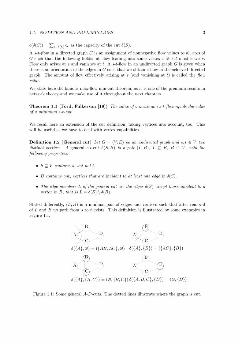
Definition 1.2 (General cut) Let G = (V,E) be an undirected graph and s, t ∈ V twodistinct vertices. A general s-t-cut δ(S,B) is a pair (L,B), L ⊆ E, B ⊂ V , with thefollowing properties:
• S ⊆ V contains s, but not t.
• B contains only vertices that are incident to at least one edge in δ(S).
• The edge members L of the general cut are the edges δ(S) except those incident to avertex in B, that is L = δ(S) \ δ(B).
Stated differently, (L,B) is a minimal pair of edges and vertices such that after removalof L and B no path from s to t exists. This definition is illustrated by some examples inFigure 1.1.
δ({A}, ∅) = ({AB,AC}, ∅) δ({A}, {B}) = ({AC}, {B})
δ({A}, {B,C}) = (∅, {B,C}) δ({A,B,C}, {D}) = (∅, {D})
A
AA
A
B
BB
B
C
CC
C
D
DD
D
Figure 1.1: Some general A-D-cuts. The dotted lines illustrate where the graph is cut.
4 CHAPTER 1. INTRODUCTION
A linear program is an optimization problem with a linear cost function, whose feasible setis defined by linear inequalities. Every linear program can be stated as
mincT x, (1.1a)
Ax ≤ b, (1.1b)
x ∈ Rn, (1.1c)
with A ∈ Rm×n, b ∈ Rm, c ∈ Rn. Note that the feasible set P = {x ∈ Rn : Ax ≤ b} alwaysdefines a polyhedron. For an introduction to linear programming we refer to [59].
A mixed integer program is a linear program with the additional constraint that specifiedvariables must take integral values. Any mixed integer program can be stated as
mincT x + dT y, (1.2a)
Ax + By ≤ b, (1.2b)
(x, y) ∈ Rn1 × Zn2, (1.2c)
with A ∈ Qm×n1 , B ∈ Qm×n2, b ∈ Qm, c ∈ Qn1, d ∈ Qn2 . The restriction to rationalconstraint coefficients is necessary to ensure that the supremum of (1.1) is attained if itexists. For a detailed introduction on mixed integer programming see [53, 59, 69]. Aninteger program is a mixed integer program with n1 = 0, i.e., it does not contain realvariables, but only integral variables. A LP-relaxation (or linear relaxation) of a mixedinteger program (1.2) is the linear program obtained by dropping the integrality constraintson the y-variables. In this thesis we assume familiarity with some basic theory on thesetopics.
Chapter 2
Problem description
Motivated by a practical application, we will describe the problem under consideration inthis chapter. We give a short survey of variants of the problem and of related work tothis class of problems. Finally, we resume some complexity results to throw light on thehardness of the problem.
2.1 Background of the problem
In the next paragraphs, we focus on optical networks, as they are the application of ourwork. We survey some properties of these networks and problems arising from their design.
2.1.1 Optical networks
Globalization and the tendency to knowledge based societies challenge many fields of sci-ence and technology. The increasing need for information exchange and communicationcapabilities yields rising demands for both technical and structural progress.
Communication is organized with hierarchical networks. On the lowest level of the hierarchy,connection demands of single users or computers are processed in a network connected tothe next higher level of the hierarchy. In this second level a whole city or region is connectedand linked to the next level and so on. On the most upper level, countries and continentsmust be connected via a wide-area network. Clearly, the traffic to be managed increasesfrom level to level. The core network (or backbone network) at top level has to handletraffic amounts in the order of terabits or even petabits per second.
Large global and national networks capable of transporting huge amounts of data are neededto meet the desired capabilities. Optical networks are telecommunication networks basedon optical, digital processing of signals. These networks provide high speed, high bandwidthdata and communication ability. Since optics are superior to previous electronic technologyin terms of speed, bandwidth, and costs, optical networks are mostly used as wide-areabackbone networks connecting continents, countries, or regions.
Optical networks consist of a set of nodes connected by optical fibers. We distinguish
5
6 CHAPTER 2. PROBLEM DESCRIPTION
different layers, depicting different aspects of the network. The physical layer contains thehardware to carry the signals and to process them on the links and in the switching nodes.Signals are fed into the network at a node, transported along the links, and arrive at someother switching node as their destination. Hence, the physical layer can be represented bya graph, where switching nodes are represented by vertices and fiber links by edges. Weconsider the links to be able to carry signals in both directions, so the graph of the physicallayer is undirected.
In first generation optical networks, the optical signal was transformed to an electronicsignal, switched, and then transmitted again as an optical signal to the next switchingnode. This optic-electronic-optic conversion (o-e-o conversion) used to be a bottleneck ofoptical networks due to the limited switching speed of electronic components. This hasbeen overcome in second generation optical networks, where the switching can be donefully optical without any o-e-o conversion. This is the reason why these networks are oftencalled all-optical networks.
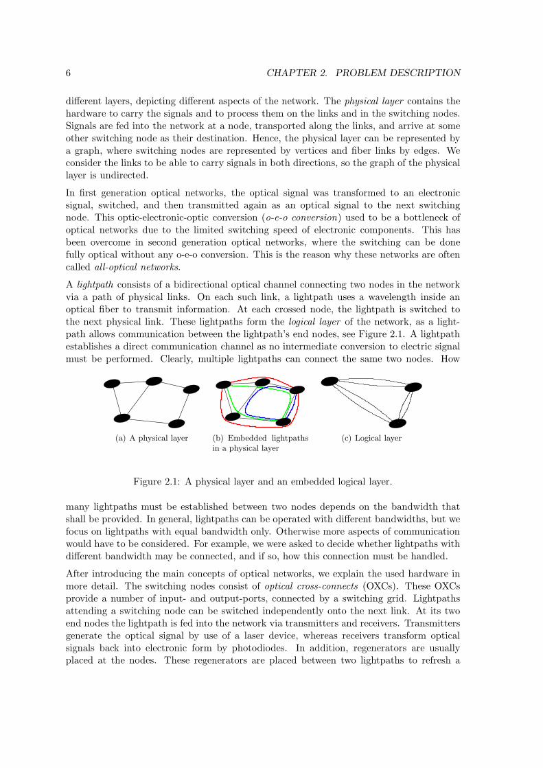
A lightpath consists of a bidirectional optical channel connecting two nodes in the networkvia a path of physical links. On each such link, a lightpath uses a wavelength inside anoptical fiber to transmit information. At each crossed node, the lightpath is switched tothe next physical link. These lightpaths form the logical layer of the network, as a light-path allows communication between the lightpath’s end nodes, see Figure 2.1. A lightpathestablishes a direct communication channel as no intermediate conversion to electric signalmust be performed. Clearly, multiple lightpaths can connect the same two nodes. How
(a) A physical layer (b) Embedded lightpathsin a physical layer
(c) Logical layer
Figure 2.1: A physical layer and an embedded logical layer.
many lightpaths must be established between two nodes depends on the bandwidth thatshall be provided. In general, lightpaths can be operated with different bandwidths, but wefocus on lightpaths with equal bandwidth only. Otherwise more aspects of communicationwould have to be considered. For example, we were asked to decide whether lightpaths withdifferent bandwidth may be connected, and if so, how this connection must be handled.
After introducing the main concepts of optical networks, we explain the used hardware inmore detail. The switching nodes consist of optical cross-connects (OXCs). These OXCsprovide a number of input- and output-ports, connected by a switching grid. Lightpathsattending a switching node can be switched independently onto the next link. At its twoend nodes the lightpath is fed into the network via transmitters and receivers. Transmittersgenerate the optical signal by use of a laser device, whereas receivers transform opticalsignals back into electronic form by photodiodes. In addition, regenerators are usuallyplaced at the nodes. These regenerators are placed between two lightpaths to refresh a
2.1. BACKGROUND OF THE PROBLEM 7
signal that uses both lightpaths. This regeneration is mainly an o-e-o conversion.
Optical fibers can carry multiple signals at the same time using wavelength division multi-plexing (WDM). That means, that different signals use different wavelengths on a fiber inparallel. In simplex fibers both directions for optical signals are realized on the same glasscore, whereas in duplex fibers the same capacity is provided in both directions by a pair ofglass cores. However, these capacities can be used only in the predetermined direction.
For each fiber a WDM system is required, essentially consisting of a multiplexer and ademultiplexer. A multiplexer bundles optical signals carried by different wavelengths andsends the combined signal onto the fiber. Entering the next node, the demultiplexer splitssuch signals in order to switch the single signals.
The optical signal is subject to signal intensity loss due to interference, attenuation, anddispersion, depending on the fiber’s quality. Consequently, the installable WDM systemsdepend on this quality, too. Moreover, the signal must possibly be amplified, reshaped, orretimed along the fiber. Unfortunately, a full signal regeneration can not be done fully opti-cal yet. That’s why there is a length bound for lightpaths depending on the hardware (e.g.,the fiber quality) and the technology used (e.g., the bit rate). If a lightpath would violatethis length bound, we must provide several lightpaths instead and a signal regenerationmust be supplied between these partial lightpaths.
Finally, wavelength conversion must be taken into account. Possibly, a lightpath can notuse the same wavelength throughout the used fibers, mainly because of limited resources.In such cases, the optical signal must be converted onto a different wavelength at somenode. Presently, no optical wavelength conversion is possible, so it is supplied by a receiver-transmitter-pair. This conversion allows a single lightpath on any wavelength to be trans-formed to any other available wavelength. In comparison to this full range conversion othertechniques may be used, e.g. limited range conversion. Here, a wavelength can only beconverted to a subset of available wavelengths, namely its spectral neighbours. Anotherpossibility is to assign conversion capability to the whole node, that is, any lightpath visit-ing this node can change its wavelength.
2.1.2 Optical network design
We next turn to the design process of optical networks. First of all, we have to definethe demands for the network. Demands in optical networks are often considered to bequasi-static. That means, the demand to be fulfilled is assumed to be static. This isdue to the fact that in backbone networks many demands from lower levels in the wholenetwork hierarchy are multiplexed. Moreover, the demands are considered as static becausechanging the logical layer is somewhat difficult. So the demands will be given, e.g., frompast requirements or forecasts. Clearly, in larger time intervals the demands can change,and even the network must be updated. Then the design process must be repeated. So itmight be part of the optical network design problem that an existing optical network has tobe extended instead of greenfield planning. Finally, the demands are specified in numbersof lightpaths needed to satisfy the actual requirements.
Demands can be directed or undirected. Undirected demands may reflect symmetrical
8 CHAPTER 2. PROBLEM DESCRIPTION
demands in both directions. Further restrictions on the routing may be considered. Forexample it can be required that symmetrical demands must be routed symmetrically, thatmeans, their lightpaths must use the same links.
Designing an optical network consists of three parts:
1. Dimensioning
Given the demands, enough hardware has to be installed to provide the necessaryrouting capacities. Possibly, this capacitation shall be done on top of an existingnetwork.
Thereby, topology decisions can be included, like decisions on which of the links canbe established at all.
There can be restrictions how much hardware of some type can be installed at aspecial site.
2. Routing
Once routing capacities are provided by the physical layer, the routing itself has tobe established. That means, given the network capacities and the network demands,the logical layer has to be set up. If needed, survivability requirements must be met.Additionally, length bounds of the lightpaths must be considered. Thus, two or morelightpaths have possibly to be routed to establish a single channel.
3. Wavelength assignment
When the routing of the lightpaths is given, a wavelength must be assigned to eachlightpath. This wavelength must be provided on all links the lightpath uses. In casethat wavelength conversion is possible, a wavelength must be provided to any link ofthe lightpath.
The main goal is usually to satisfy all demands at least cost, where costs arise for each(newly) installed hardware component. Minimizing the costs is naturally the network op-erator’s goal. Although all three tasks described above influence each other, solving themaltogether is usually a very hard problem. The hardness of the design process arises fromthe fact that many decisions must be made, so the design problem yields naturally largeinstances with respect to the number of singular decisions. Addionally, the relations be-tween all these decisions are complicated, and the incorporation of costs and the objectivecomplicates the design problem even more. Because of the hardness of the design prob-lem decomposing the problem is a common approach. That is, dimensioning, routing, andwavelength assignment are carried out sequentially. Some research deals with solving twoof the mentioned parts together. Usually though this is still hard for relevant instance sizes,i.e., arising in real world networks.
We next focus on survivability concepts. Survivability means to ensure that the impact ofnetwork failures is as low as possible within reasonable additional costs. Due to its highperformance nature, a break-down of even a single component may lead to dramatic lossof traffic capability of the network. Survivability concepts affect the dimensioning of thenetwork and the routing. In the dimensioning part enough capacities must be provided to
2.2. SPECIFICATION 9
admit an appropriate routing. In the routing part such a routing must be established thatfulfils the survivability requirements.
Different approaches were made to keep the impact of network failures as low as possible.Among them are path-restoration, link-restoration, and diversification, see [68] for an in-troduction. The latter concept will be considered in this work. Diversification is a conceptthat bounds the traffic through any network link or node of any demand. So, a break-downof one component of the network can only affect a certain portion of each demand.
2.2 Specification
In this section we will state the problem under consideration in this work. As alreadymentioned, the network design problem is very hard, so decomposing this problem is areasonable approach. We use the decomposition mentioned in Section 2.1.2. Our workfocus on the routing problem, that is part of the overall network design problem.
Within the dimensioning process the physical layer has been determined. So we are given asupply graph G = (V,E) associated with the physical layer. For each established link thereis an edge in E, and for each switching node there is a vertex in V .
By the installation of fibers and WDM systems, routing capacity is provided at the links.We regard all routing capacities as homogeneous. That is, we neither distinguish betweenchannels of different WDM systems and fibers of the same link, nor do we distinguishbetween channels of the same WDM system. Hence, for any edge e ∈ E there is anassociated edge capacity ce. This edge capacity is defined by the number of lightpaths thatcan be routed across the link associated with e. All edge capacities are positive integers, asall hardware is addressed to whole optical channels only, see Section 2.1.1.
Similarly, by the installation of OXCs there is a routing capacity for all nodes. Each pairof input and output ports in an OXC admits the routing of one lightpath through theswitching node. The routing capacity of a node is the number of lightpaths that can crossthe node. For each node there is an associated vertex v ∈ V , and the routing capacity ofthe node yields a vertex capacity cv. Since we deal with port pairs, the vertex capacity isagain a positive integer.
After we have described the supply graph, we next describe how demands are incorporated.The demands are given by an undirected demand graph H = (T, F ), where the nodes T ⊆ Vare called terminals. We denote by Q the set of demands or commodities. To any demandk ∈ Q, there is an associated demand edge fk ∈ F with end nodes sk and tk. Additionally,there is a demand value dk, an integer describing the number of lightpaths to be routedbetween sk ∈ T and tk ∈ T . Finally, we have a diversification parameter ρk ∈ (0, 1] for eachdemand k ∈ Q.
The objective is to find a maximum number of sk-tk-paths in G, but at most dk for eachdemand k. Each path consumes one unit of capacity on each edge and node it crosses,including its end terminals. The overall set of lightpaths must not exceed the mutual edgeand node capacities given. That means, the number of paths crossing an edge or vertex isbound by the edge or vertex capacity, respectively, regardless of the demand the paths are
10 CHAPTER 2. PROBLEM DESCRIPTION
serving.
Furthermore, the set of paths belonging to a single demand k has to fulfil the diversificationrequirements, that is, no more than ⌊ρkdk⌋ of these lightpaths use the same edge or vertex,except the end terminals of this demand. This ensures that in case of a failure in anyphysical link or node (except sk, tk) at least dk − ⌊ρkdk⌋ paths survive for demand k. Ofcourse a failure of sk or tk causes the loss of all paths for this demand.
A maximum number of paths has to be established at minimum cost. In the network designproblem as stated in Section 2.1.2 we don’t consider costs of routings. However, in orderto use the resources “economically” we aim to find routings that use as few capacities aspossible. Note, that free capacities can be used for future enlargements of demands. Thereis still another advantage of saving capacities: if some node or link carries less paths, thena failure at this component will break less paths.
To minimize the utilization we assign costs to it. We aim to minimize the overall utilizationof only the edges. Since the number of vertices touched by a path depends on the numberof edges it passes, the utilization of vertices is already considered implicitly. That’s why wewill not take vertex utilization into account for the cost function explicitly. Formally, eachpath P causes lP cost units. Recall that lP is the number of edges of the path.
The routing of each demand can be seen as a network flow. For that, we consider sk as asource of commodity k. Additionally, tk is the target of commodity k. We aim to send flowfrom the source to the target, and at all vertices in between no flow can vanish or arise.As we are interested in whole paths only, the flow of any commodity on any edge must beintegral. The integral flow for each demand can be decomposed in a number of paths andcycles. Since we want to obtain a lightpath routing, we restrict the flow for every demandto be cycle-free. That means, the flow must be decomposable into paths only.
The mutual capacity constraints for the path routing correspond directly to capacity con-straints for flows. That means, that all flow sent through any vertex or edge by any demandmust not exceed the vertex’ or edge’s capacity.
As the main ingredients of our problem are the integrality, the multicommodity flow struc-ture, and the node capacities, from here on we will denote our problem as IMCF-N.
2.3 Variations of the problem
The above specified problem can be varied in many ways. We want to outline some variationsof the multicommodity flow problem. These variations concern different flow definitions,different mutual capacity constraints, different graph structures, or different objectives.Among the different flow types described in literature we mention fractional flows, integralflows, and unsplittable flows. Widely studied objectives are maximum flow, minimum costflow, minimum congestion flow, and maximum concurrent flow. Graph structures of interestare therefore planar graphs and graphs with even degree of every vertex. Another possibilityis to subdivide multicommodity flow problems for directed and undirected graphs. Sincemany combinations of objectives, flows, and special graph structures are possible, a widevariety of problems may arise.
2.3. VARIATIONS OF THE PROBLEM 11
Fractional multicommodity flow
The somewhat “standard” multicommodity flow problem concerns directed supply and de-mand graphs. This can be seen as the base problem, since undirected supply edges anddemands can usually be modelled in a directed setting, see [1] for the basic ideas of thetransformation. Thus the demand’s terminals become sinks and sources, indicating wherethe paths start and end. Furthermore, no vertex capacities are assumed, as capacitatedvertices can be modelled as (directed) edges, see again [1]. In this variant, no diversifica-tion or other survivability constraints are given, as such constraints heavily depend on theapplication. Finally we may drop the integrality constraint, this means that any path cancarry some arbitrary positive amount of flow instead of just one unit. This is why the term’fractional’ is in the problem’s name. The flows of each demand can be generalized furtherto admit multiple sinks and sources for each commodity.
Unsplittable multicommodity flow
In the unsplittable multicommodity flow problem (also called non-bifurcated flow problem),the routing of each demand has to use only one path in the network. We might have tochoose to route the whole demand on a single path or not, or we’re allowed to route anyfraction of the demand on its single path. Unsplittable flows can be considered with specifieddemands, for example in computer networks, but usually no demand values are given.
Edge-disjoint paths
Another classical problem is the edge-disjoint paths problem. Given an, usually undirected,graph and a (multi-)set of vertex pairs, we want to find a maximum number of pathsconnecting these vertex pairs. These paths must be edge-disjoint. This problem can beseen as an integer multicommodity flow problem, and generalizes naturally to an integerunsplittable flow problem, when taking edge capacities and demand values into account. Tosee this, assume we have an integral multicommodity flow problem where edge capacitiesare given. Then we can replace an edge with edge capacity ce by ce parallel edges with unitcapacity. If demands are specified, we can do the same replication in the demand graph.
Next we mention some objectives that can be applied.
Maximum multicommodity flow (Max MCF)
In a maximum multicommdity flow, no demand values are specified. The objective is tomaximize the sum of flow established between any terminal pair.
Minimum cost multicommodity flow (MinCost MCF)
Here, it is assumed that all demands can be satisfied. The aim is to find a feasible routingof all demands at least cost, with respect to some cost function. Note, that our problemIMCF-N can be seen as a two stage combination of MaxMCF and MinCost MCF, as we
12 CHAPTER 2. PROBLEM DESCRIPTION
first want to find a maximum flow, and then to obtain this maximum flow with minimumcost.
Minimum congestion flow (MinCong)
In this variant, specified demands must be completely satisfied. We consider the congestionof edges, that is the ratio of utilization of the edge and its capacity. The congestion θ ofthe whole network is the maximum congestion of the edges. This network congestion shallbe minimized. If the edge capacities are ce for edge e, a congestion θ means that edgecapacities θce would suffice to fulfil all demands without overutilization. This is a matter ofinterest in computer network communication, as we consider to route the all commodities in⌈θ⌉ rounds. In our problem IMCF-N, a routing would be feasible if the network congestionis less than or equal to one.
Maximum concurrent flow (MaxConc)
Here, we are interested in the portion of each demand that can be routed in the network.That is, we want to maximize the concurrent λ, where λdk of each demand shall be routed.The minimum congestion flow problem can be seen as equivalent to the maximum concurrentflow problem, as a network congestion θ allows to route θ−1 of the demands, and a flowwith concurrent λ yields a routing of the whole demands with congestion λ−1.
2.4 Related work
As there are many variants of the problem, and quite a lot of mathematical formulationsfor them, a wide spread research related to the problem has been done. We give a shortsurvey on the work about theoretical aspects, approximation algorithms, and proposedsolution methods. This survey whatsoever does not claim to be exhaustive. For a moredetailed survey on such results and related topics see [44]. The considerations given hereaim to explain the hardness of our problem IMCF-N, and to outline the variety of solutionapproaches.
First, we want to state the cut condition, as it is of crucial importance throughout therest of this work. It is closely related to the max-flow min-cut theorem, but extending tomulticommodity flows.
Definition 2.1 Let G = (V,E) be a graph with edge capacities ce for every edge e ∈ E. Letthere be a demand graph H as described in Section 2.2, defining q demands. The demandshave terminals si, ti and a positive real number demandi specifying the demand value ofdemand i.
Let the min-ratio cut be given by
ρ∗ = min∅6=S⊂V
∑
e∈δG(S) ce∑
f∈δH(S) df.
2.4. RELATED WORK 13
The cut condition holds, when ρ∗ ≥ 1
In simple words, the cut condition holds when the capacity of any cut is at least as largeas the demand separated by the cut. We easily see that for q = 1 the cut condition isequivalent to the existence of a s1-t1-flow of value d1, due to the max-flow min-cut theorem1.1.
2.4.1 Complexity
Before investigating the problem under consideration, we classify it and some variants interms of complexity. We first reflect the hardness of the considered problem and thenprovide related results.
First of all, the fractional multicommodity problem with any objective function is solvable inpolynomial time, since it can be formulated as a linear program with a polynomial numberof variables and inequalities, and linear programming is solvable in polynomial time withthe ellipsoid method [30].
The maximum edge-disjoint paths problem is known to be NP-hard, see [25]. If we usea diversification parameter ρ = 1 for all demands and set the vertex capacities arbitraryhigh, and set the demand values dk arbitrary high for all demands, our problem IMCF-Nturns out to be the maximum edge-disjoint paths problem. Since we can conclude that themaximum edge-disjoint path is contained in IMCF-N, our problem is NP-hard as well.
The integer maximum multicommodity flow problem was proven to be MAX SNP-hard forundirected graphs, see [26]. That is, there is no polynomial approximation scheme for thisproblem unless P = NP . Moreover, Ma and Wang [50] showed that this problem cannot be
approximated for directed graphs within ratio 2log1−ǫ n unless NP ⊆ DTIME[2polylog(n)].Here, polylog(k) denotes a function asymptotical bounded by some polynomial of fixeddegree of log(k) (to put it differently: polylog(k) := logO(1) k).
Additionally, for every fixed nonnegative integer K it is still NP-complete to decide whetheran instance is solvable with the demand values decreased by K, even when the original in-stance is fractionally solvable. Furthermore, the maximum integer multicommodity problemis MAX SNP-hard even when G is a tree and the edge capacities are large (i.e. ce ≥ C withC ∈ O(poly(m)) ), see [65]. Similar to the notation used above, poly(k) denotes kO(1).
2.4.2 Theoretical results
A series of results deals with the max-flow min-cut ratio for fractional multicommodityflows. This ratio describes how large the min-ratio cut must be to allow all demands tobe satisfied. The max-flow min-cut ratio is defined by κ∗ = ρ∗
θ∗ , where θ∗ is the maximumconcurrent. Clearly, κ∗ ≥ 1, since on every cut δG(S) we need capacity at least as large asthe portion θ∗ of the separated demands. Plotkin and Tardos [57] were the first to showan upper bound on κ∗ independent of the capacities and demand values. They obtainedan approximation of O(q2) for κ∗. This result was improved to O(q) by Aumann andRabani [4]. Finally, Gunluk [31] showed that κ∗ is O(q∗) when q∗ > 1, where q∗ is the
14 CHAPTER 2. PROBLEM DESCRIPTION
cardinality of the minimal vertex cover of the demand graph. The improvement of the lastbound can be seen when considering a demand graph consisting of two stars, spanning allvertices of V . Then q = |V | − 2, but q∗ = 2. Gunluk also showed that his bound is tight inthe sense that for any n ∈ N there is an instance with n vertices, where this bound is tightup to a constant.
There is a famous characterization of the solvability of fractional multicommodity flows withspecified demands. Here, solvability means that all demands must be fully satisfied. Theresult is based on duality theory of linear programming, and extends the (obviously neces-sary) cut condition to a sufficient condition for solvability of the fractional multicommodityflow problem.
Theorem 2.2 (Kakusho and Onaga, [39]; Iri, [38]) A capacity vector c yields a feasi-ble multicommodity flow if and only if
∑
e∈E
µece ≥∑
k∈Q
πkdk, (2.1)
for all edge weights µe, e ∈ E. Here, πk is the value of a shortest sk-tk path in G withrespect to the edge weights µ.
The inequalities (2.1) are called metric inequalities, and play an important role for thedimensioning problem of networks, see for example [68].
We next turn to integral flows. As mentioned above, integral flows can be seen as the ques-tion for edge-disjoint paths connecting predefined terminal pairs. In case of one commodity,the maximum edge-disjoint paths problem was considered as early as 1927 by Menger [52].He proved that the maximum number of edge-disjoint s-t paths in a graph G for two verticess, t in G is equal to the minimum number of edges in a s-t cut.
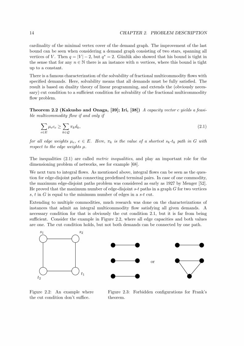
Extending to multiple commodities, much research was done on the characterizations ofinstances that admit an integral multicommodity flow satisfying all given demands. Anecessary condition for that is obviously the cut condition 2.1, but it is far from beingsufficient. Consider the example in Figure 2.2, where all edge capacities and both valuesare one. The cut condition holds, but not both demands can be connected by one path.
s1 s2
t1t2
Figure 2.2: An example wherethe cut condition don’t suffice.
or
Figure 2.3: Forbidden configurations for Frank’stheorem.
2.4. RELATED WORK 15
Among other results, Frank [23] proved the following characterization: if all edge capaci-ties are integral and the demand graph does not contain any of the two configurations infigure 2.3, then the cut condition is equivalent to the existence of a half-integral multi-commodity flow. A half-integral multicommodity flow is a multicommodity flow where theflows of all demands on all edges are a half of an integer. Excluding the configurations infigure 2.3 means that the demand graph is either (i) the complete graph K4, (ii) the circuitC5, or (iii) the union of two stars.
We next mention some results dealing with planarity of the incorporated graphs and theparity condition. The parity condition holds when for all vertices v in the supply graph∑
vw∈E cvw +∑
i∈Q:v∈{si,ti}di is even, that is when the capacities of all edges adjacent to v
has the same parity as the demand emanating at v. Here, Q is again the set of demands andthe di are given demand values. Considering an integral multicommodity flow problem asan edge-disjoint paths problem by the replication construction mentioned above, the paritycondition states that G ∪H is Eulerian.
Okamura and Seymour [55] showed, that if the supply graph G is planar, the parity conditionholds, and all demand terminals lie on the boundary of some face of G, then the cut conditionis equivalent to the existence of an integral multicommodity flow satisfying all demands.The proof given by the authors is constructive, yielding an algorithm of finding such amulticommodity flow. Wagner and Weihe [67] improved this to an algorithm with linearrunning time in the number of vertices. Okamura [54] weakened his result to the conditionthat the demand terminals may lie on two boundaries of faces of G, but both terminals ofany demand must lie on the same of the two boundaries.
Finally, we consider the case when G∪H is planar. In this case, and if the parity conditionholds, then there is an integral multicommodity flow satisfying all demands if and only ifthe cut condition holds, see [61]. When we don’t assume the parity condition, similar resultshold. If G∪H is planar and the number of demands is fixed (or bounded), Sebo [60] showedthat the integer multicommodity flow problem is polynomially solvable. Finally, the twolast mentioned results were generalized by Korach and Penn [43]. In case G ∪H is planarand if the cut condition holds, they gave a polynomial time construction of a solution.
We say that G is inner Eulerian, if the sum of capacities of the edges adjacent to some non-terminal vertex is even, for all non-terminal vertices. Among other results, Karzanov [40]showed that for inner Eulerian supply graphs together with the condition, that the graphof anticliques A(H) of H is bipartite, the problem has an integer-valued optimal solution,for a simpler proof see [24]). The anticliques of the demand graph are the maximal, withrespect to inclusion, independent vertex sets of H. The graph of the anticliques has a vertexfor every anticlique of H, and an edge between two such vertices when the correspondinganticliques have a common terminal in H. A(H) is said to be bipartite if its vertice set canbe partitioned into two independent sets. Karzanov gave a polynomial time algorithm con-structing such a solution, too. Examples of such demand graphs are for instance completegraphs.
Summing up the result presented here, we can conclude that easy solvable instances arerare, and we can not hope that such instances for our problem IMCF-N might appear.
16 CHAPTER 2. PROBLEM DESCRIPTION
2.4.3 Research on approximation
Skutella [63] gave approximations for the unsplittable multicommodity flow problem. Inthe version under his consideration all demands have to share a common source vertex. Inthis case it is still NP-complete to decide whether all demands can be satisfied, since itcontains the knapsack problem. The approximations obtained for various objectives likeminimum congestion, maximum flow are all constant factor approximations.
Baveja and Srinivasan [8] studied approximation algorithms for the integer unsplittable flowproblem, and obtained an O(
√m) approximation, where m is the number of edges in the
graph. If the objective value is large enough, i.e. if it is larger than m, they could evenshow a Θ(1) approximation.
In [64], the integral minimum congestion problem, both in unsplittable and splittable set-ting, is studied by Srinivasan. Supply graphs and demand graphs may be directed orundirected. Using the Randomized Rounding approach, they get an 1+ o(1) approximationwhen the fractional solution, that is the minimum congestion without fixing the flows tointegers, grows faster than log m. Randomized Rounding relies on the idea of roundingfractional solutions due to some sophisticated rounding scheme, that exploits the structureof both constraints and objectives.
Fleischer [18] gave the fastest polynomial approximation schemes for fractional multicom-modity flow problems to this day. Most important, for the maximum multicommodity flowproblem, their algorithm’s runtime is independent of the number of commodities. When nocosts are given, the approximation schemes are fully polynomial.
For the maximum integral multicommodity flow problem, Garg, Vazirani, and Yannakakis [26]gave a 1
2 -approximation. In the version they considered no demand values are specified, andthe objective is to maximize the total demand that can be fulfilled. The supply graph isrestricted to be a tree.
2.4.4 Research on solution methods
A general introduction to solution methods for fractional multicommodity flow problemscan be found in [41, 1], the latter from a more modern point of view. A survey on models andsolution approaches for rail transportation can be found in [3]. In rail transportation usuallya timetable has to be served at minimum cost. Costs arise by routings for trains and possiblyby extending the capacities of the track network. When the capacities may be extendedwe obtain an extension of multicommodity flow problems, known as multicommodity fixedcharge network design problem. In terms of Section 2.1.2, the dimensioning and routingproblem is solved together. The same railway routing problem is considered in [10], too,where the instances are solved by simulated annealing.
In [51], McBride and Mamer solved the fractional multicommodity problem on undirectedgraphs. They exploited the undirected structure within a formulation with piecewise linearconvex objective and constraints. They modified the primal simplex algorithm to deal withthis convexity. Additionally, they proposed a special pricing procedure, thus keeping thesize of the formulation relatively small. An exploitation of the simplex method with similar
2.4. RELATED WORK 17
ideas is given in [17]. The main goal of the authors is to keep the matrices involved incomputation small. They interpret the derived data structures in terms of the originalnetwork structures.
The computational results in [51] suggest that their approach is superior to standard tech-niques for the undirected setting. Such standard techniques mostly deal with directed graphsderived from the original undirected graph, leading to larger graphs than the original graph.In Section 3.2 we give an example for such constructions.
Barnhart, Hane, and Vance [7] studied a branch-and-price algorithm for solving the integerminimum cost unsplittable multicommodity flow problem. They used a path based formula-tion and proposed a branching rule based on arc flows. They point out that their approachoutperforms standard branching rules.
Alvelos and de Carvalho [2] extended this idea to problems without the unsplitting con-straint. Their results show that this approach is competitive to an edge based formulationsolved with a standard integer programming code.
A more general integer multicommodity flow problem arising as a transportation prob-lem in the airplane industry is studied in [66]. The extra difficulties are due to the factthat commodities can not be shipped independently from each other, producing nonlinearside constraints. Both approximation and exact solution methods are proposed. The ex-act approach is a branch-and-price algorithm working on a path based formulation, thusovercoming the problem of nonlinear constraints.
Lobel [48] studied vehicle scheduling problems, and derived a minimum cost integer multi-commodity flow model with unit demands for them. He obtained an integer program via anedge-flow formulation, that was solved by branch-and-cut. His solution approach includedcolumn generation schemes as well as Lagrangian relaxations to obtain lower bounds. TheLagrangian relaxations were solved by a subgradient method. He reported promising resultsfor instances with up to 25000 commodities.
In [22] bundle methods are used to solve minimum cost fractional multicommodity flowproblems. Bundle methods are extensions of subgradient methods that we study in chap-ter 4. The authors applied their codes on so called cost-decomposition formulations, andfound them competitive to general purpose LP-solvers. The bundle approach is extended tomulticommodity fixed charge network design problems in [13]. There, the LP relaxation ofof a typical edge-flow formulation (see Section 3.2.1) had to be solved. Again, the authorsfound the bundle methods to be superior to a standard linear programming techniques likesimplex and barrier optimizers.
The short survey in this section shows that due to the large number of variations of mul-ticommodity flow problems many solution approaches have been considered. Up to thispoint, no approach superior to any other can be detected.

18 CHAPTER 2. PROBLEM DESCRIPTION
Chapter 3
Model and formulations
In this chapter we present a model for the problem IMCF-N introduced in chapter 2 andformulate the optimization task as several integer programs. We examine some propertiesof the underlying mathematical objects, namely polyhedra, to motivate why we use thepresented formulations.
3.1 Model
As already pointed out in Section 2.2, we can model the desired routing as network flows,one for each commodity. Network flows are extensively studied objects in combinatorialoptimization and well understood. For a survey see e.g., [1]. A flow of commodity k ∈ Q isa map that assigns a flow value and a direction to every edge of the supply graph. So, forevery edge vw, a flow for demand k determines which amount of commodity k is shippedfrom v to w or from w to v.
For every commodity k, we assign a deficit of commodity k to every vertex. The deficit ofcommodity k at some vertex v determines how much the flow towards v must exceed theflow away from v. This property is called flow conservation, since no flow vanishes or raisesexcept to balance the vertex deficits.
In section 2.2 we defined light paths and routings as undirected. We consider directed flowsonly, essentially because modelling undirected flows is much more circumstantial than fordirected flows. The direction of flows has no influence on their treatment with respect tocapacities. Since we deal with directed flows only, we have to assign an arbitrary directionto every demand.
The variable ak describes how many of the dk desired paths can not be established, andhence how much flow cannot be sent from sk to tk. We model the terminal sk as a source offlow where an excess of dk − ak is located, and assign a deficit of −(dk − ak) of commodityk to sk. The second terminal tk is modelled as the target of the flow for demand k, and weassign a deficit of dk − ak to it. All other vertices except sk and tk are assigned a deficit0 with respect to commodity k. The reason for introducing variables ak instead of, e.g.,variables for the flow really sent, is that on the one hand we want to minimize the flow
19
20 CHAPTER 3. MODEL AND FORMULATIONS
costs. On the other hand, we want to maximize the flow sent between the commodity’sterminals. To incorporate both goals the latter one is modelled as to minimize the flow notsent. So both goals are minimizing objectives.
The objective is firstly to route as much demand as possible, and secondly to minimize theedge utilization, without any preference among the commodities or edges.
The first goal is equivalent to minimize the sum of the ak, while the second goal is equivalentto minimize the sum of edge flows for every commodity. To control the trade-off betweenthe two goals, the ak are assigned a cost coefficient M , while the cost coefficients for alledge flows are 1. A large value of M emphasizes on minimizing the demand not served,while a small M emphasizes to save capacities. The problem specified in section 2.2 asksfor a maximum satisfaction of the demands as a primary goal. How large should M be toprovide this emphasis on routing demands? As any path connecting two terminals couldonly use |V | − 1 edges without crossing any node twice, M = |V | suffices. Choosing thisvalue for M , self-intersecting paths with more than |V | edges can not occur in an optimalsolution. However, this does not destroy the emphasis on demand satisfaction. Supposewe are given an optimal solution, and there is a self-intersecting path p satisfying anotherunit of demand. Then clearly p contains cycles. Leaving out p’s cycles yields a shorterpath p′ with at most |V | − 1 edges. The new path p′ without cycles will not utilize anyedge or vertex more than the original path p does. So p′ can be used instead of p, andthe objective-driven restriction to paths with at most |V | does not affect the validity of ourmodel.
As already mentioned, while minimizing the edge utilization we also minimize the nodeutilization. The node utilization depends directly on the edge utilization, since a path usingt edges will use exactly t + 1 nodes.
A well known property of network flows is that such a flow can be decomposed into a setof paths and cycles, see e.g., [9] for an algorithm for that decomposition. Moreover, thealgorithms for such a decomposition task have polynomial running time. Note however,that this decomposition is not unique, that means, a flow for some commodity can bedecomposed into paths and cycles in several ways.
As we stated the problem in section 2.2, the flow of every commodity must be cycle-free. Inthe presented models, we do not restrict explicitly the flows to be cycle-free. The reason forthis relaxation is that we can derive a cycle-free flow from any given flow easily. Supposewe are given a flow for some commodity k, and we decompose it in a number of paths andcycles. By simply dropping the cycles we obtain a new flow for commodity k, that doesnot use more edge and node capacities than the originally given flow. Moreover, as anycycle contains edges, dropping the cycles will decrease the cost for the commodity’s flow.Clearly, as we keep all paths of the flow decomposition, we sent the same amount of thecommodity k from sk to tk. Note, that in an optimal multicommodity flow the flow of everycommodity is already cycle-free. If any of the flows for the particular commodities containcycles, dropping these cycles would lead to a better solution.
Finally, in our model we meet the diversification requirements by bounding the flow ofcommodity k through vertices and edges to ⌊ρkdk⌋, except at the vertices sk, tk. Since theflows are directed, we are able to determine how much flow of a particular commodity enters
3.2. FORMULATIONS 21
or leaves some vertex. Note that for all commodities, the flow of commodity k entering tkutilizes tk, while the flow of commodity k leaving sk utilizes sk. Measuring utilization thisway reflects the fact that paths consume capacity at their terminals, too. At all othervertices (except sk, tk) the in-flow equals the out-flow of commodity k, so utilization can bemeasured from both in-flow and out-flow. Obviously, each commodity needs its own flowbounds.
3.2 Formulations
Here, we give some formulations of the model above as integer linear programs and as aninteger convex program. We state the standard edge-flow based formulation that we willuse to compare with the two formulations we extensively study. The former will be usedas a benchmark for our approach. For the sake of completeness we state a path-flow basedformulation as mentioned in section 2.4. Finally, we introduce the two formulations basedon resource-directed decomposition. These will be the formulations to be studied further inChapters 4 & 5.
3.2.1 Edge-flow based formulation
The most common idea for modelling multicommodity flow problems is a flow formulationwith edge variables. We use variables fk
(vw), fk(wv) to denote the flow of commodity k ∈ Q
on edge vw ∈ E in the direction from v to w or from w to v, respectively. Note, thatwe distinguish between fk
(vw) and fk(wv), although the edge vw ∈ E is equal to the edge
wv ∈ E. The variables ak describe the amount of demand k that cannot be satisfied. The
22 CHAPTER 3. MODEL AND FORMULATIONS
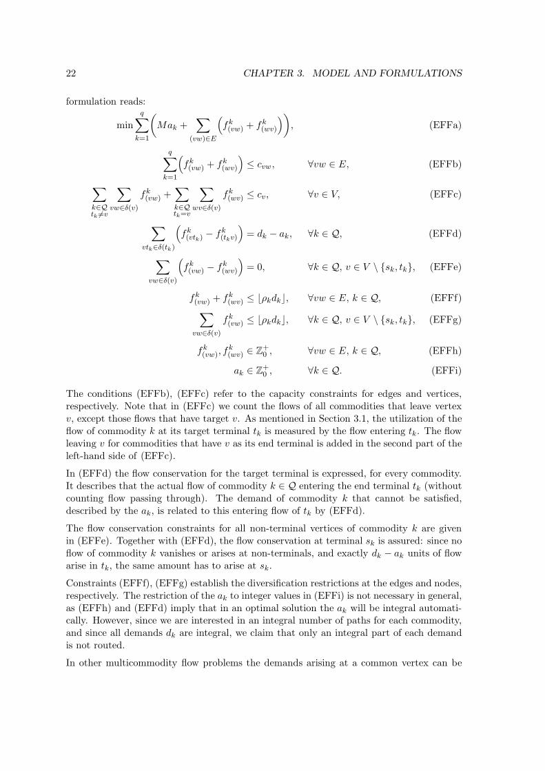
formulation reads:
min
q∑
k=1
(
Mak +∑
(vw)∈E
(
fk(vw) + fk
(wv)
)
)
, (EFFa)
q∑
k=1
(
fk(vw) + fk
(wv)
)
≤ cvw, ∀vw ∈ E, (EFFb)
∑
k∈Qtk 6=v
∑
vw∈δ(v)
fk(vw) +
∑
k∈Qtk=v
∑
wv∈δ(v)
fk(wv) ≤ cv, ∀v ∈ V, (EFFc)
∑
vtk∈δ(tk)
(
fk(vtk) − fk
(tkv)
)
= dk − ak, ∀k ∈ Q, (EFFd)
∑
vw∈δ(v)
(
fk(vw) − fk
(wv)
)
= 0, ∀k ∈ Q, v ∈ V \ {sk, tk}, (EFFe)
fk(vw) + fk
(wv) ≤ ⌊ρkdk⌋, ∀vw ∈ E, k ∈ Q, (EFFf)∑
vw∈δ(v)
fk(vw) ≤ ⌊ρkdk⌋, ∀k ∈ Q, v ∈ V \ {sk, tk}, (EFFg)
fk(vw), f
k(wv) ∈ Z+
0 , ∀vw ∈ E, k ∈ Q, (EFFh)
ak ∈ Z+0 , ∀k ∈ Q. (EFFi)
The conditions (EFFb), (EFFc) refer to the capacity constraints for edges and vertices,respectively. Note that in (EFFc) we count the flows of all commodities that leave vertexv, except those flows that have target v. As mentioned in Section 3.1, the utilization of theflow of commodity k at its target terminal tk is measured by the flow entering tk. The flowleaving v for commodities that have v as its end terminal is added in the second part of theleft-hand side of (EFFc).
In (EFFd) the flow conservation for the target terminal is expressed, for every commodity.It describes that the actual flow of commodity k ∈ Q entering the end terminal tk (withoutcounting flow passing through). The demand of commodity k that cannot be satisfied,described by the ak, is related to this entering flow of tk by (EFFd).
The flow conservation constraints for all non-terminal vertices of commodity k are givenin (EFFe). Together with (EFFd), the flow conservation at terminal sk is assured: since noflow of commodity k vanishes or arises at non-terminals, and exactly dk − ak units of flowarise in tk, the same amount has to arise at sk.
Constraints (EFFf), (EFFg) establish the diversification restrictions at the edges and nodes,respectively. The restriction of the ak to integer values in (EFFi) is not necessary in general,as (EFFh) and (EFFd) imply that in an optimal solution the ak will be integral automati-cally. However, since we are interested in an integral number of paths for each commodity,and since all demands dk are integral, we claim that only an integral part of each demandis not routed.
In other multicommodity flow problems the demands arising at a common vertex can be
3.2. FORMULATIONS 23
aggregated, that means that they are merged into a single demand. This has the advantagethat less demands have to be considered, while multiple sinks are established. This approachis not possible for our problem due to the diversification constraints. We could not decidewhich amount of flow of an aggregated demand crosses an edge or vertex.
An obvious disadvantage of formulation (EFF) is that in some optimal solution at most oneof the variables in the pairs fk
(vw), fk(wv) will be positive. If both variables of such a pair would
be positive, they would form a cycle flow that can be removed. That is the reason why weexamine some more formulations. We consider some more properties of formulation (EFF)in Section 3.3, when we compare it to another formulation given in Section 3.2.3.
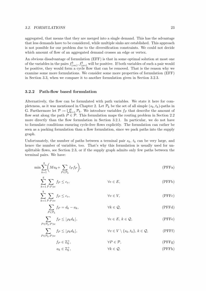
3.2.2 Path-flow based formulation
Alternatively, the flow can be formulated with path variables. We state it here for com-pleteness, as it was mentioned in Chapter 2. Let Pk be the set of all simple (sk, tk)-paths inG. Furthermore let P :=
⋃qk=1Pk. We introduce variables fP that describe the amount of
flow sent along the path P ∈ P. This formulation maps the routing problem in Section 2.2more directly than the flow formulation in Section 3.2.1. In particular, we do not haveto formulate conditions ensuring cycle-free flows explicitly. The formulation can rather beseen as a packing formulation than a flow formulation, since we pack paths into the supplygraph.
Unfortunately, the number of paths between a terminal pair sk, tk can be very large, andhence the number of variables, too. That’s why this formulation is usually used for un-splittable flows, see Section 2.3, or if the supply graph admits only few paths between theterminal pairs. We have:
min
q∑
k=1
(
Mak+∑
P∈Pk
lP fP
)
, (PFFa)
q∑
k=1
∑
P :P∋e
fP ≤ ce, ∀e ∈ E, (PFFb)
q∑
k=1
∑
P :P∋v
fP ≤ cv, ∀v ∈ V, (PFFc)
∑
P∈Pk
fP = dk − ak, ∀k ∈ Q, (PFFd)
∑
P∈Pk:P∋e
fP ≤ ⌊ρkdk⌋, ∀e ∈ E, k ∈ Q, (PFFe)
∑
P∈Pk:P∋v
fP ≤ ⌊ρkdk⌋, ∀v ∈ V \ {sk, tk}, k ∈ Q, (PFFf)
fP ∈ Z+0 , ∀P ∈ P, (PFFg)
ak ∈ Z+0 , ∀k ∈ Q. (PFFh)
24 CHAPTER 3. MODEL AND FORMULATIONS
Note that lP describes the length of path P , that is the number of edges the path uses.(PFFb),(PFFc) formulate the mutual capacity constraints for edges and vertices in G, re-spectively. The desired number of paths connecting the various terminal pairs are describedin (PFFd). The diversification restrictions are stated in (PFFe) for edges and in (PFFf) forvertices. For the integrality constraints (PFFh) on the ak, the same remark holds equallyas for the formulation (EFF) in the previous section: integrality is forced by the otherconstraints.
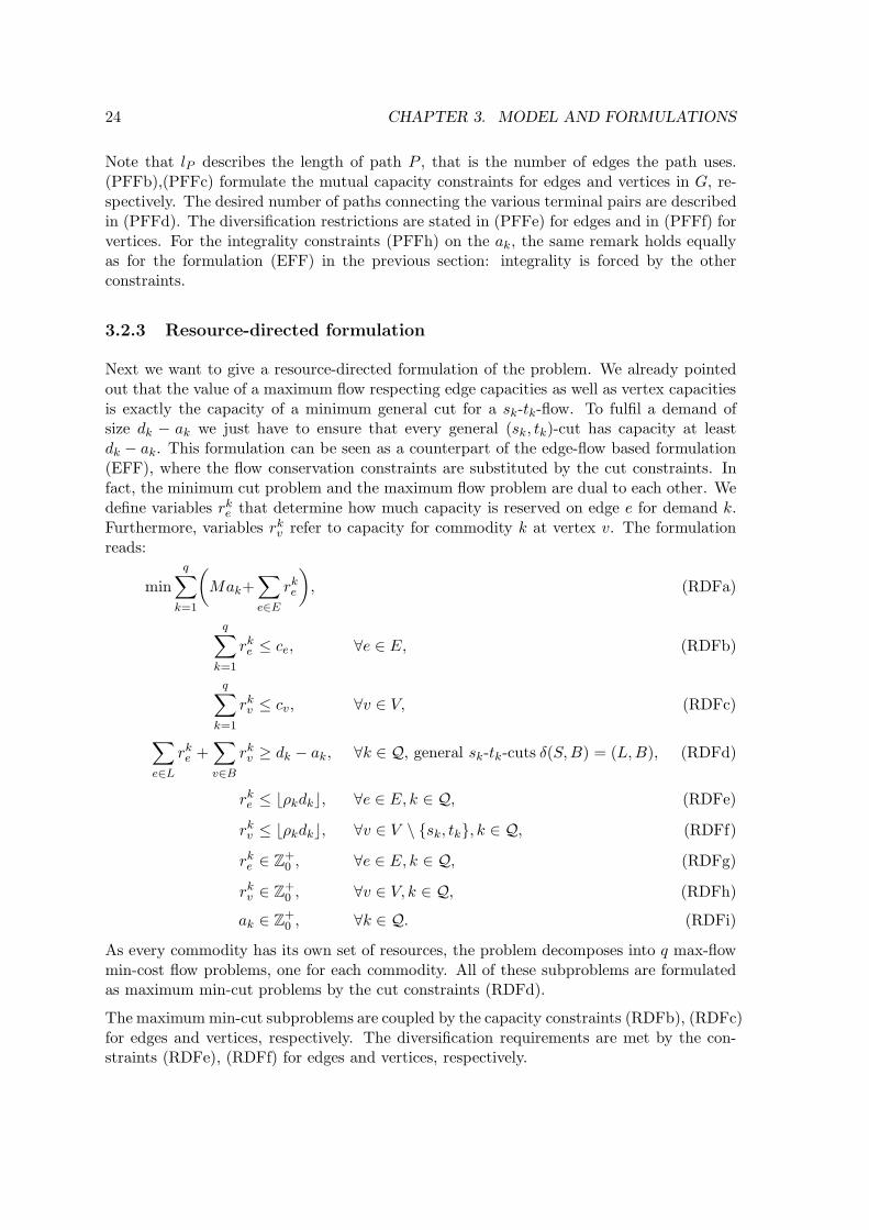
3.2.3 Resource-directed formulation
Next we want to give a resource-directed formulation of the problem. We already pointedout that the value of a maximum flow respecting edge capacities as well as vertex capacitiesis exactly the capacity of a minimum general cut for a sk-tk-flow. To fulfil a demand ofsize dk − ak we just have to ensure that every general (sk, tk)-cut has capacity at leastdk − ak. This formulation can be seen as a counterpart of the edge-flow based formulation(EFF), where the flow conservation constraints are substituted by the cut constraints. Infact, the minimum cut problem and the maximum flow problem are dual to each other. Wedefine variables rk
e that determine how much capacity is reserved on edge e for demand k.Furthermore, variables rk
v refer to capacity for commodity k at vertex v. The formulationreads:
min
q∑
k=1
(
Mak+∑
e∈E
rke
)
, (RDFa)
q∑
k=1
rke ≤ ce, ∀e ∈ E, (RDFb)
q∑
k=1
rkv ≤ cv, ∀v ∈ V, (RDFc)
∑
e∈L
rke +
∑
v∈B
rkv ≥ dk − ak, ∀k ∈ Q, general sk-tk-cuts δ(S,B) = (L,B), (RDFd)
rke ≤ ⌊ρkdk⌋, ∀e ∈ E, k ∈ Q, (RDFe)
rkv ≤ ⌊ρkdk⌋, ∀v ∈ V \ {sk, tk}, k ∈ Q, (RDFf)
rke ∈ Z+
0 , ∀e ∈ E, k ∈ Q, (RDFg)
rkv ∈ Z+
0 , ∀v ∈ V, k ∈ Q, (RDFh)
ak ∈ Z+0 , ∀k ∈ Q. (RDFi)
As every commodity has its own set of resources, the problem decomposes into q max-flowmin-cost flow problems, one for each commodity. All of these subproblems are formulatedas maximum min-cut problems by the cut constraints (RDFd).
The maximum min-cut subproblems are coupled by the capacity constraints (RDFb), (RDFc)for edges and vertices, respectively. The diversification requirements are met by the con-straints (RDFe), (RDFf) for edges and vertices, respectively.
3.2. FORMULATIONS 25
Using general cuts to formulate conditions for a feasible flow of a certain amount has theadvantage that we need only one variable for every edge and commodity. Recall that in theedge-flow formulation (EFF) we introduced two variables for each edge and commodity. Onthe other hand, in formulation (RDF) we have variables for every vertex and commodity,too, but not in formulation (EFF). However, the supply graph G has at least as many edgesas vertices, except when G is a tree. Hence, the formulation (RDF) has less variables thanformulation (EFF) whenever G contains more than |V | edges.
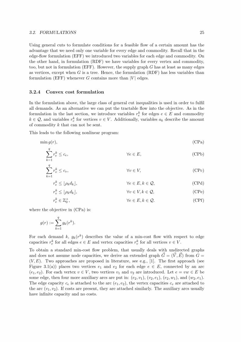
3.2.4 Convex cost formulation
In the formulation above, the large class of general cut inequalities is used in order to fulfilall demands. As an alternative we can put the tractable flow into the objective. As in theformulation in the last section, we introduce variables rk
e for edges e ∈ E and commodityk ∈ Q, and variables rk
v for vertices v ∈ V . Additionally, variables ak describe the amountof commodity k that can not be sent.
This leads to the following nonlinear program:
min g(r), (CPa)
q∑
k=1
rke ≤ ce, ∀e ∈ E, (CPb)
q∑
k=1
rkv ≤ cv , ∀v ∈ V, (CPc)
rke ≤ ⌊ρkdk⌋, ∀e ∈ E, k ∈ Q, (CPd)
rkv ≤ ⌊ρkdk⌋, ∀v ∈ V, k ∈ Q, (CPe)
rke ∈ Z+
0 , ∀e ∈ E, k ∈ Q. (CPf)
where the objective in (CPa) is:
g(r) :=
q∑
k=1
gk(rk).
For each demand k, gk(rk) describes the value of a min-cost flow with respect to edge
capacities rke for all edges e ∈ E and vertex capacities rk
v for all vertices v ∈ V .
To obtain a standard min-cost flow problem, that usually deals with undirected graphsand does not assume node capacities, we derive an extended graph ~G = (~V , ~E) from G =(V,E). Two approaches are proposed in literature, see e.g., [1]. The first approach (seeFigure 3.1(a)) places two vertices e1 and e2 for each edge e ∈ E, connected by an arc(e1, e2). For each vertex v ∈ V , two vertices v1 and v2 are introduced. Let e = vw ∈ E besome edge, then four more auxiliary arcs are put in: (e2, v1), (v2, e1), (e2, w1), and (w2, e1).The edge capacity ce is attached to the arc (e1, e2), the vertex capacities cv are attached tothe arc (v1, v2). If costs are present, they are attached similarly. The auxiliary arcs usuallyhave infinite capacity and no costs.
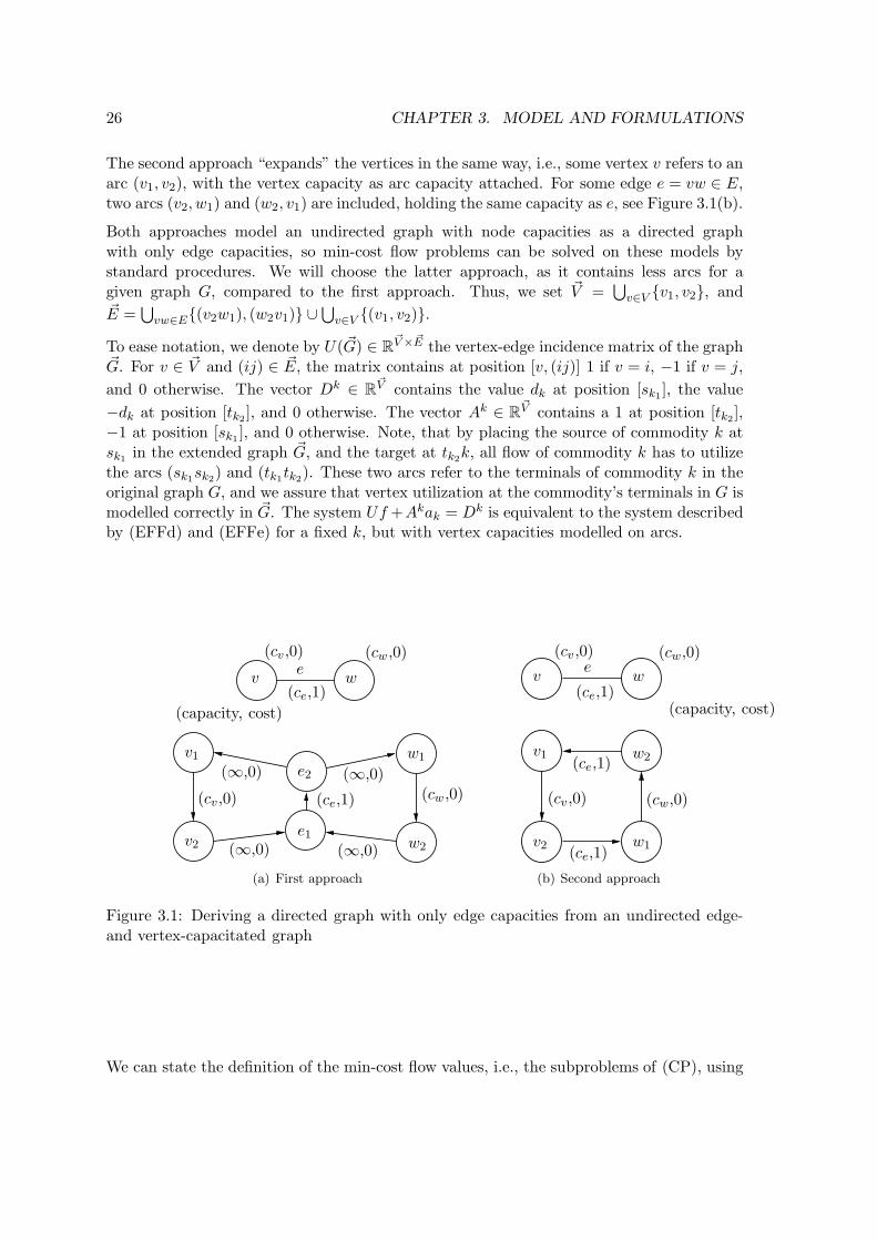
26 CHAPTER 3. MODEL AND FORMULATIONS
The second approach “expands” the vertices in the same way, i.e., some vertex v refers to anarc (v1, v2), with the vertex capacity as arc capacity attached. For some edge e = vw ∈ E,two arcs (v2, w1) and (w2, v1) are included, holding the same capacity as e, see Figure 3.1(b).
Both approaches model an undirected graph with node capacities as a directed graphwith only edge capacities, so min-cost flow problems can be solved on these models bystandard procedures. We will choose the latter approach, as it contains less arcs for agiven graph G, compared to the first approach. Thus, we set ~V =
⋃
v∈V {v1, v2}, and~E =
⋃
vw∈E{(v2w1), (w2v1)} ∪⋃
v∈V {(v1, v2)}.
To ease notation, we denote by U( ~G) ∈ R~V × ~E the vertex-edge incidence matrix of the graph
~G. For v ∈ ~V and (ij) ∈ ~E, the matrix contains at position [v, (ij)] 1 if v = i, −1 if v = j,
and 0 otherwise. The vector Dk ∈ R~V contains the value dk at position [sk1
], the value
−dk at position [tk2], and 0 otherwise. The vector Ak ∈ R
~V contains a 1 at position [tk2],
−1 at position [sk1], and 0 otherwise. Note, that by placing the source of commodity k at
sk1in the extended graph ~G, and the target at tk2
k, all flow of commodity k has to utilizethe arcs (sk1
sk2) and (tk1
tk2). These two arcs refer to the terminals of commodity k in the
original graph G, and we assure that vertex utilization at the commodity’s terminals in G ismodelled correctly in ~G. The system Uf +Akak = Dk is equivalent to the system describedby (EFFd) and (EFFe) for a fixed k, but with vertex capacities modelled on arcs.
v w
v1
v2
w1
w2
e
e1
e2
(ce,1)
(cv ,0) (cw,0)
(capacity, cost)
(cv ,0) (cw,0)
(∞,0) (∞,0)
(∞,0) (∞,0)
(ce,1)
(a) First approach
v w
v1
v2 w1
w2
e
(ce,1)
(cv ,0) (cw,0)
(capacity, cost)
(ce,1)
(ce,1)
(cv ,0) (cw,0)
(b) Second approach
Figure 3.1: Deriving a directed graph with only edge capacities from an undirected edge-and vertex-capacitated graph
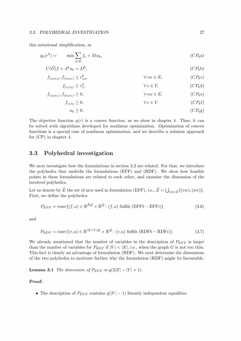
We can state the definition of the min-cost flow values, i.e., the subproblems of (CP), using
3.3. POLYHEDRAL INVESTIGATION 27
this notational simplification, as
gk(rk) = min
∑
e∈E
fe + Mak, (CPka)
U( ~G)f + Akak = Dk, (CPkb)
f(v2w1), f(w2v1) ≤ rkvw, ∀ vw ∈ E, (CPkc)
f(v1v2) ≤ rkv , ∀ v ∈ V, (CPkd)
f(v2w1), f(w2v1) ≥ 0, ∀ vw ∈ E, (CPke)
fv1v2≥ 0, ∀ v ∈ V (CPkf)
ak ≥ 0. (CPkg)
The objective function g(r) is a convex function, as we show in chapter 4. Thus, it canbe solved with algorithms developed for nonlinear optimization. Optimization of convexfunctions is a special case of nonlinear optimization, and we describe a solution approachfor (CP) in chapter 4.
3.3 Polyhedral investigation
We next investigate how the formulations in section 3.2 are related. For that, we introducethe polyhedra that underlie the formulations (EFF) and (RDF). We show how feasiblepoints in these formulations are related to each other, and examine the dimension of theinvolved polyhedra.
Let us denote by E the set of arcs used in formulation (EFF), i.e., E =⋃
vw∈E{(vw), (wv)}.First, we define the polyhedra
PEFF = conv{(f, a) ∈ REQ × RQ : (f, a) fulfils (EFFb− EFFi)} (3.6)
and
PRDF = conv{(r, a) ∈ R(E+V )Q × RQ : (r, a) fulfils (RDFb− RDFi)}. (3.7)
We already mentioned that the number of variables in the description of PEFF is largerthan the number of variables for PRDF if |V | < |E|, i.e., when the graph G is not too thin.This fact is clearly an advantage of formulation (RDF). We next determine the dimensionsof the two polyhedra to motivate further why the formulation (RDF) might be favourable.
Lemma 3.1 The dimension of PEFF is q(2|E| − |V |+ 1).
Proof.
• The description of PEFF contains q(|V | − 1) linearly independent equalities.
28 CHAPTER 3. MODEL AND FORMULATIONS
It is a well known fact that the edge-node incidence matrix U( ~G) has row rank |V |−1,see [1] Theorem 11.10. Thus, for each k ∈ Q, the constraints (EFFd), (EFFe) establish|V |−1 linearly independent equalities. Obviously, these sets of equalities are altogetherlinearly independent, since each set incorporates only variables of a single demand.
• There are q(2|E| − |V |+ 1) + 1 affinely independent feasible points in PEFF .
Consider, for each k ∈ Q, the setting ak = dk − 1. Furthermore, let ai = dk, andf i
vw = f iwv = 0, for all i ∈ Q \ {k}. Under these assumptions, to obtain a feasible
point of PEFF , we have to establish a single path for demand k. As already pointedout the matrix U( ~G) has row rank of |V | − 1. As all other constraints like nodeconstraints (EFFc) and diversification constraints (EFFf),(EFFg) are redundant, weyield 2|E| − |V |+ 1 linearly independent flow vectors for demand k, establishing thedesired path. Note, that U( ~G) is totally unimodular, see e.g., [69, Proposition 3.4].Thus, the integrality constraints can be satisfied by the linearly independent flowvectors.
As for all k ∈ Q such a setting can be obtained, and as the sets of linearly independentflow vectors are altogether linearly independent, this yields q(2|E| − |V |+ 1) linearlyindependent points in PEFF . Together with the point fk
vw = fkwv = 0 for all vw ∈ E,
k ∈ Q, ak = dk for all k ∈ Q, we get the desired q(2|E| − |V | + 1) + 1 affinelyindependent feasible points in PEFF .
As we have q(2|E|+ 1) variables, the lemma follows. �We next show that PRDF is full-dimensional.
Lemma 3.2 The dimension of PRDF is q(|E|+ |V |+1), that is, PRDF is full-dimensional.
Proof. We proof the lemma straight forward by constructing q(|E|+ |V |+ 1) + 1 affinelyindependent feasible points of PRDF .
For all demands k ∈ Q and all ν ∈ E ∪ V we define a feasible point pk,ν as follows: first weset pk,ν [rk
ν ] = 1, and for all η ∈ (E ∪ V ) \ {ν} we set pk,ν[rkη ] = 0. We denote by p[ri
η] theentry for the variable ri
η in the point p. For all other demands i 6= k and all η ∈ E ∪ V we
set pk,ν[riη] = 0. We set pk,ν[ai] = di for all demands i ∈ Q. Clearly, all points generated
this way are feasible for (RDF), hence contained in PRDF .
For every demand k we define another feasible point pk,◦ quite similar: for all ν ∈ E ∪V setwe set pk,◦[rk
ν ] = 1, for all other demands i 6= k we set pk,◦[riν ] = 0. The variables ai for
not routed demands are set to pk,◦[ak] = dk − 1, and for all other demands i 6= k we setpk,◦[ai] = di.
Finally, we provide another feasible point p•. This point is given by p•[riν ] = 0 for all
demands i and all ν ∈ E ∪ V , and p•[ai] = di.
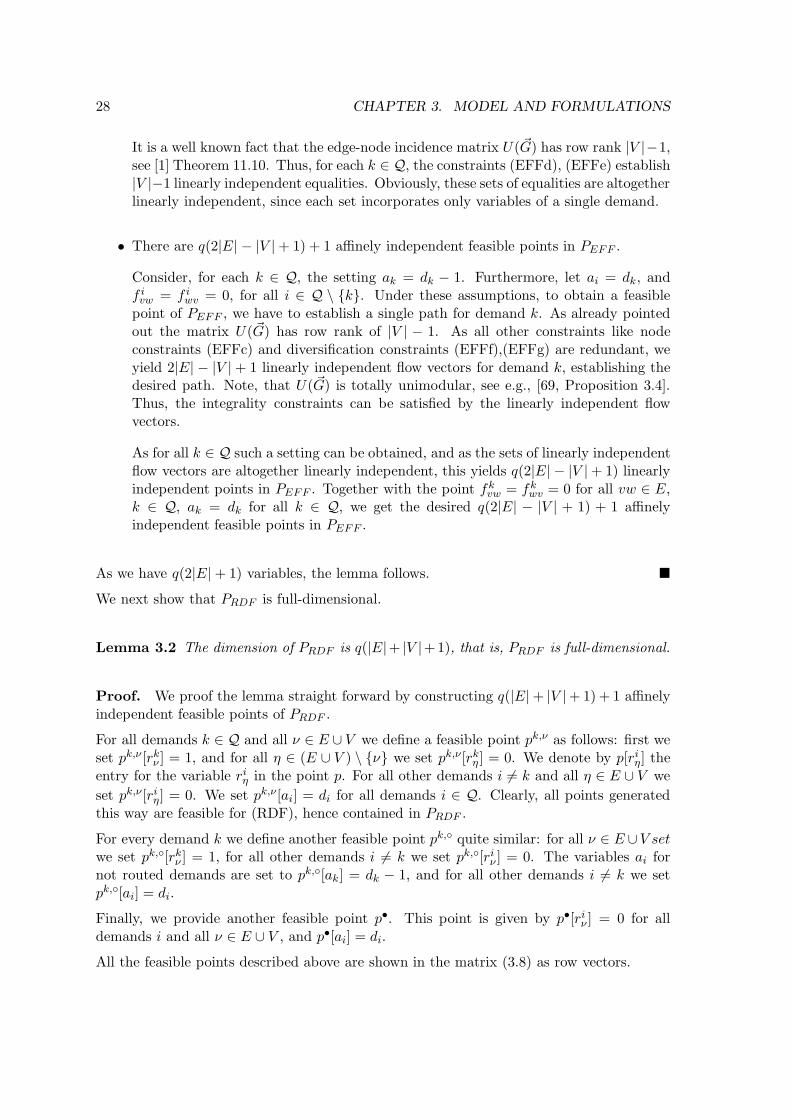
All the feasible points described above are shown in the matrix (3.8) as row vectors.
3.3. POLYHEDRAL INVESTIGATION 29
1 d1 . . . dq
. . ....
...1 d1 . . . dq
. . ....
1 d1 . . . dq
. . ....
...1 d1 . . . dq
1T d1 − 1 . . . dq
. . .. . .
1T d1 . . . dq − 1
0T d1 . . . dq
(3.8)
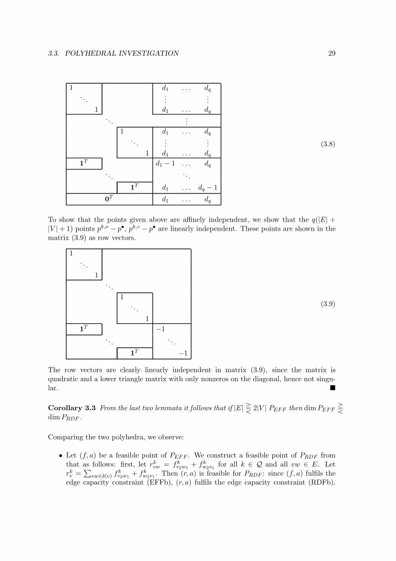
To show that the points given above are affinely independent, we show that the q(|E| +|V |+ 1) points pk,ν − p•, pk,◦ − p• are linearly independent. These points are shown in thematrix (3.9) as row vectors.
1. . .
1. . .
1. . .
1
1T −1
. . .. . .
1T −1
(3.9)
The row vectors are clearly linearly independent in matrix (3.9), since the matrix isquadratic and a lower triangle matrix with only nonzeros on the diagonal, hence not singu-lar. �
Corollary 3.3 From the last two lemmata it follows that if |E| T 2|V | PEFF then dimPEFF Tdim PRDF .
Comparing the two polyhedra, we observe:
• Let (f, a) be a feasible point of PEFF . We construct a feasible point of PRDF fromthat as follows: first, let rk
vw = fkv2w1
+ fkw2v1
for all k ∈ Q and all vw ∈ E. Letrkv =
∑
vw∈δ(v) fkv2w1
+ fkw2v1
. Then (r, a) is feasible for PRDF : since (f, a) fulfils theedge capacity constraint (EFFb), (r, a) fulfils the edge capacity constraint (RDFb).
30 CHAPTER 3. MODEL AND FORMULATIONS
By construction, the vertex capacity constraints (EFFc) for (f, a) imply that (r, a)fulfils the vertex capacity constraints (RDFc). The min-cut max-flow theorem 1.1 inits general form with vertex capacities applies to the flow fk for each commodity k:if such a flow fk established by (EFFd), (EFFe) admits sending dk − ak units of flowfrom sk to tk, every general sk-tk cut has a capacity of at least dk − ak. Hence, (r, a)satisfies the general cut restrictions (RDFd). Finally, (r, a) meets the diversificationconstraints (RDFe), (RDFf), since (f, a) fulfils the diversification constraints (EFFf),(EFFg).
• A reverse relation does not hold. Of course, given a feasible point (r, a) of PRDF ,we can compute a feasible point (f, a) by solving q max flow problems with edgecapacities rk
vw and node capacities rkv on the graph G. Especially, we can yield the
same values for the ak. However, increasing some variable rkvw or rk
v not in a minimalgeneral cut for demand k may lead to another feasible point of PRDF , but the point(f, a) obtained from that will stay the same. On the other hand, given edge and noderesources rk
vw and rkv as total flow values on edges and through nodes, possibly more
than one directed flow can be obtained. E.g., circular (partial) flows can be reversedyielding the same total flow on all edges and nodes.
Chapter 4
Subgradient method
In this chapter we introduce some basic ideas of the subgradient method. We will statesome known results, not in general as such but fitted to our aim. We outline several variantswhich are all suitable for a relaxation of our problem. Then we show how this method canbe applied to our problem. Finally, we extend the method to produce heuristically integralsolutions.
4.1 Theoretical framework
The subgradient method was first proposed by Shor [62]. It generalizes the idea of gra-dients of differentiable functions. The subgradient method aims to find optimal solutionsof minimization problems with convex objective function, or maximization problems withconcave objective function. It can be used only when the objective function is continu-ous and defined on a simply connected subset of a finite dimensional vector space. As anapproximation approach, it only provides convergence to optimal solutions under certainconditions. Nevertheless, it has been shown to be valuable for various problems, often beingsuperior to other approaches. Additionally, it is easy to implement in comparison to othersolution techniques, for example a modern simplex algorithm. The subgradient method’sfirst successful application was to solve the Lagrangian Dual of the Traveling SalesmanProblem by Held and Karp [32, 33]. As a consequence, non-differentiable convex program-ming became a field of theoretical and practical interest on its own. In our context, theconcepts presented here are only a starting point for this kind of algorithms.
In this section, we first mention some general ideas of subgradient methods, as developedfor convex programs without side constraints. Afterwards we give some ideas from litera-ture on how this can be extended to programs with additional constraints, namely linearinequalities, as this is the case in our model.
31
32 CHAPTER 4. SUBGRADIENT METHOD
4.1.1 General scheme
The general idea of the subgradient method can be described as follows: suppose we aregiven a function defined on a proper ground set, that shall be minimized. Furthermore, let astarting point be given in the ground set. We aim to find a direction of decreasing functionvalue. Furthermore, we have to determine a step length to move along the chosen direction.Iterating this process should end in a point that is (at least approximately) optimal for theproblem. In the simplest case where the objective is a convex function to minimize, andthis objective is defined on a whole vector space, every local minimum is a global minimum.
From analysis of differentiable function it is known that the gradient of a differentiablefunction points in the direction of local steepest ascent at every point where the gradient isevaluated. So it is a natural choice to move in the direction of the negative gradient. In thecase of non-differentiability, where no gradient is available, we have to generalize the ideato subgradients, that still keeps the main properties needed for the optimization process.
A subgradient is defined as follows:
Definition 4.1 A subgradient at some point x for a convex function f : Rn → R is avector γ(x) such that f(ν) ≥ f(x) + γ(x)T (ν − x) for all ν ∈ Rn.
Let f be a convex function defined on Rn. Then a convex program is to find a point in Rn,if such one exists, that minimizes f . The subgradient method works as follows: provided astarting point x1 ∈ Rn, a sequence {xk} is computed according to
xk+1 = xk − hkγ(xk)
‖γ(xk)‖ ∀ k ∈ N (4.1)
where γ(ν) is a subgradient of f at the point ν and {hk} is a sequence of positive steplengths. Note that this is exactly the idea mentioned above: we choose the direction ofthe negative subgradient and move along this direction to get a new point. To obtainconvergence of the sequence {xk} to a global minimum, the following theorem is essential,see [58]:
Theorem 4.2 (Polyak) Let f : Rn → R be a convex function. Let there be an arbitrarystarting point x1 ∈ Rm, and a sequence {xk} defined by (4.1). Let the sequence of steplengths be such
limk→∞
hk = 0,
k∑
j=1
hjk→∞−→ ∞
hold. Then
Φk := min1≤j≤k
f(xj)k→∞−→ min
x∈Rnf(x).
4.1. THEORETICAL FRAMEWORK 33
For the step lengths many approaches are used, e.g.:
hk =h
k ln k, hk =
h
kβ, 0 < β ≤ 1, hk =
h
k + C, (4.2)
where h is a starting step length, while β and C are constants. These approaches differin the speed of convergence of the hk to zero, and in the way the sum of the step lengthsincreases. The right choice of the step lengths is crucial in the convergence behaviour ofa subgradient method, but the best choice heavily depends on the problem, the instancecharacteristics, the starting step length, and the initial point x1. Although the step lengthsin (4.2) assure convergence due to Theorem 4.2, they did not satisfy in practice. Usuallythe speed of convergence is too low. That’s why in practice the step length h is dividedby a constant factor β1 (often 2 is recommended) due to some heuristic. For example, ifthe best objective value reached so far has not been improved for β2 iterations, β2 beinganother positive constant, h is lowered this way. Note that this setting can not guaranteeconvergence in general.
Finally, the step length can be chosen dependent only on the current point and subgradient.For that, a line search along γ(xk) is carried out to find (approximately) the step lengthleading to a new point that minimizes the objective function on the ray from xk alongγ(xk). However, although this procedure assures convergence and can decrease the numberof iterations needed, there is a trade-off between the decreased number of iterations and theincreased expense in each iteration due to the multiple objective evaluation.
Another extension widely used is not to take only the subgradient at the current pointto compute the next point, but to take the predecessor, too. To use the information ofsubgradients of former iterations is part of the wide field of bundle methods. These methodsthough reach beyond the scope of this work. For a detailed introduction to bundle methodssee e.g., [35, 46]. However, a straight forward approach is to use a direction gk instead ofγ(xk) in (4.1), defined as:
gk = γ(xk) + σkgk−1, σk ∈ R. (4.3)
Here, σk describes the influence of the preceding direction onto the new direction in the kthiteration. For that, σk ≥ 0 should be set. Note that (4.1) describes the special case whenσk = 0 for all k ∈ N. There are several such subgradient adjusting rules that differ in theway σk is set:
• Crowder rule
Here, σk is fixed to some constant value < 1. The rule was proposed by Crowderin [15].
• Camerini-Fratta-Maffioli rule
This is a more sophisticated rule, motivated by the idea, that a vastly “jumping”direction should be smoothened. It was proposed in [12], and was supported byexperimental experience in [14]. The rule states:
σk =
{
τγ(xk)T gk−1/‖gk−1‖2, if γ(xk)
T gk−1 < 0,
0, otherwise,
34 CHAPTER 4. SUBGRADIENT METHOD
where τ ∈ R is a parameter. If τ is properly chosen in the interval [0, 2], the direc-tion gk is at least as good as γ(xk) in the following sense: in the important caseif γ(xk)
T gk−1 < 0, the preceding direction gk−1 and the new subgradient γ(xk)form an angle ϕ of more than π/2, since γ(xk)
T gk−1 = ‖γ(xk)‖‖gk−1‖ cos ϕ. Con-sider again (4.3), and applying the Camerini-Fratta-Maffioli rule for the case whenγ(xk)
T gk−1 < 0 yields:
gk = ‖γ(xk)‖( γ(xk)
‖γ(xk)‖ − τ cos ϕgk−1
‖gk−1‖)
. (4.4)
In that case, we observe that the direction of gk is chosen as an affine combination ofthe directions of γ(xk) and gk−1. We further observe that:
ϕ −→ π
2⇒ gk −→ γ(xk),
ϕ −→ π ⇒ gk −→ ‖γ(xk)‖( γ(xk)
‖γ(xk)‖ + τgk−1
‖gk−1‖)
.
This observation means that τ controls the influence of the direction of gk−1 on thedirection of gk if ϕ is large. In any case the length of gk is mainly determined by thelength of γ(xk). Hence, the Camerini-Fratta-Maffioli rule aims to prevent the sub-gradient method from “zigzagging” when succeeding subgradients form large angles.The authors proposed τ = 1.5 as a reasonable choice.
• Modified Camerini-Fratta-Maffioli rule
Here, the parameter τ is dynamically adjusted to −‖γ(xk)‖‖gk−1‖/γ(xk)T gk−1, whicharises from geometrical reasons. Thus, the influence parameter becomes
σk =
{
‖γ(xk)‖/‖gk−1‖, if γ(xk)T gk−1 < 0,
0, otherwise.
In Chapter 6 we apply the rules on our problem IMCF-N and examine the impact of thedifferent rules on the obtained solutions.
In the light of the preceding outline we mention two more step length schemes. Suppose wehave a lower bound f of the optimal solution of the convex program. Crainic, Frangioni,and Gendron [14] proposed the following step lengths:
hk = λk(f(xk)− f)/γ(xk)T gk, (4.5)
which can be seen as an extension of the step lengths proposed by Kennington and Shalaby[42], who used the formula
hk = λk(f(xk)− f)/γ(xk)T γ(xk), (4.6)
and the simple setting gk = γ(xk). In both step length schemes (4.5), (4.6) the sequence{λk} assures convergence of the step lengths to zero. For that, the sequence {λk} is chosenas a nonincreasing sequence of positive real numbers converging to zero. The authorsof [14, 42] propose that, beginning with a given start value λ1, λk is divided by a constant
4.1. THEORETICAL FRAMEWORK 35
factor β1 every time the objective value f(xk) has not been improved for β2 consecutiveiterations. The authors of [34] divided λk by β1 = 2 every β2 iterations, independentlyfrom the behaviour of the objective value. We apply the step length scheme (4.5) in ourimplementation of the subgradient method. The concrete setting of the constants β1, β2,and the initial prefactor λ1 is described in Section 4.2.1.
4.1.2 Constrained programs
We extend this general subgradient schemes to problems with linear inequalities as sideconstraints, as this happens to be the case for our formulation (CP). First we formallystate the problem, then we sketch the methods to deal with the constraints. These methodscan roughly be classified as penalizing methods and projecting methods. As above, werestrict ourselves to methods that will be used in the run up.
Let f : Rn → R be a convex function. We define a constrained convex program as:
minf(x)
gi(x) ≥ 0, ∀i ∈ [m](CCONV)
Let the feasible region of (CCONV) be denoted by
X = {x|x ∈ Rn, gi(x) ≥ 0,∀i ∈ [m]}. (4.8)
To ease the following considerations and to stay close to our problem, in the sequel we willassume that the constraint functions gi are affine functions, i.e. gi(x) = aT
i x − bi, withai ∈ Rn, bi ∈ R. We investigate how the subgradient method can be extended to dealwith the additional conditions. We focus on penalty function, barrier functions, and exactpenalty functions. The application of these methods within a subgradient method for ourproblem IMCF-N is described in Section 4.2. It should be mentioned that a variety ofadditional methods were suggested, see [5] for a survey.
Penalty functions
The general idea of penalty functions for constrained programs is to relax the constraints,but to “penalize” points outside the feasible region of the program. The penalty given to allinfeasible points should be large enough to assure that the unconstrained penalized programhas only optimal solutions that are feasible.
Given a problem (CCONV) with feasible region X, we define a loss function for this problemby
s(x)
{
= 0, x ∈ X
> 0, x /∈ X.(4.9)
That means, that a loss function indicates the infeasible region where a penalty has to be
36 CHAPTER 4. SUBGRADIENT METHOD
provided. A typical setting for a loss function is
s(x) =m∑
i=1
|min{0, gi(x)}|β ,
where β is usually 1 or 2. The idea behind this example is that the loss function s increasesif the violation of some constraint increases. To choose a polynomial of low degree in sis inspired by the fact that it is easy to compute and it grows not too fast (e.g., as anexponential function) with the violation of constraints. The latter fact is important toavoid numerical difficulties.
Let {ρk} be a strictly decreasing sequence of positive numbers, called guidance parameters,and let t be a real-valued guidance function such that ρ1 > ρ2 > 0 implies t(ρ2) > t(ρ1) > 0.That means that t is positive and strictly decreasing for positive guidance parameters.Furthermore, let
limk→∞
ρk = 0 (4.10)
limk→∞
t(ρk) = +∞ (4.11)
Then t(ρk)s(x) is called an (exterior) penalty function, and the augmented objective functionis
F (x, pk) = f(x) + t(ρk)s(x). (4.12)
The penalty function is zero on the feasible set X by (4.9), and positive on the infeasible setRn \X due to (4.9) and (4.10). We get a sequence of unconstrained problems, denoted by(CONVk), that consist of finding a minimum of F (x, ρk). The desired behaviour of penaltyfunctions, i.e., leading to optimal solutions that are feasible and optimal for (CCONV), isprovided by the following theorem, see [5], Theorem 12.2.:
Theorem 4.3 (Avriel) Let the feasible set X of (CCONV) as defined in (4.8) be non-empty. Suppose there exists an ǫ > 0 such that the set
Xǫ = {x|x ∈ Rn, gi(x) ≥ −ǫ,∀i ∈ [m]}
is compact. Also suppose that the F (x, ρk) as given in (4.12) attain their unconstrainedminima on Rn for all k. Then there exists a convergent subsequence {xki∗} of the optimalsolutions to (CONVk), and the limit of any such convergent subsequence is optimal for(CCONV).
It should be noted that the assumption in Theorem 4.3, that the F (x, ρk) attain theirminima is a rather strong condition. Among other conditions to fulfil this requirement itis sufficient that all the F (x, ρk) are convex and Xǫ is compact for some ǫ > 0, as provenby Zangwill [70]. Convexity of F (x, ρk) can be established by convexity of the penaltyfunctions t(ρk)s(x), since the objective function f is convex. In addition, as we deal withaffine functions gi only, boundedness of Xǫ implies compactness of Xǫ. This boundednesscan not be established a priori, but only dependent on the specific problem. For example, ifXǫ is not bounded for any ǫ > 0, one could modify the program (CCONV) by introducingnew constraints that do not exclude all optimal solutions.
4.1. THEORETICAL FRAMEWORK 37
Barrier functions
Penalty functions penalize leaving the feasible region X as described in the section above.Another approach is to keep the sequence of generated points away from the boundary ofX. For that, feasible points are increasingly penalized when approaching the boundary.This idea is provided by so-called barrier functions.
First, we assume some regularity conditions on the program (CCONV), that read:
1. Let the interior of the X, denoted by X0, be nonempty.
2. There is a point x0 ∈ X with f(x0) = α0 such that the level setS(f, α0) = {x|x ∈ Rn, f(x) = α0} fulfils that S(f, α0) ∩ X is a com-pact set.
(4.13)
Let s be a real-valued interior loss function of x ∈ Rn such that s is continuous on X0.Furthermore, for every sequence {xk} in X0 converging to some boundary point of X, aninterior loss function s has to satisfy limk→∞ s(xk) = +∞. Also, let t be a real-valuedguidance function of ρ ∈ R such that
ρ1 > ρ2 > 0 =⇒ t(ρ1) > t(ρ2) > 0,
limk→∞
ρk = 0 =⇒ limk→∞
t(ρk) = 0.
Similar to the penalty function approach, ρk ∈ R are guidance parameters. The functiont(ρk)s(x) is a barrier function, sometimes also called interior penalty function. The aug-mented objective function obtained is
G(x, ρk) = f(x) + t(ρk)s(x). (4.14)
Thus, we again obtain a sequence of unconstrained programs, denoted by (CONVk), thatconsist of finding a minimum of G(x, ρk), without side constraints. For this barrier-type pro-grams a similar convergence result holds as for the penalty-type programs, see [5], Theorem12.3.:
Theorem 4.4 (Avriel) Let a problem (CCONV) be given with feasible set X as definedin (4.8). Assume the regularity conditions (4.13) are satisfied and the loss function s usedin the augmented objective function are positive in X0. Suppose that the G(x, ρk) attaintheir unconstrained minima in X0 for all k. If {ρk} is a strictly decreasing sequence ofpositive numbers converging to zero, then there exists a convergent subsequence {xki∗} ofthe optimal solutions to (CONVk), and the limit of any such convergent subsequence isoptimal for (CCONV).
Due to [5], a sufficient condition that all the G(x, ρk) attain their minima in X0 is that Xis bounded and X0 is not empty. Note that this holds only in the special case of linearinequalities as side constraints.
38 CHAPTER 4. SUBGRADIENT METHOD
Exact penalty functions
Given a problem (CCONV), the solution approaches introduced in the last two sectionsconstruct sequences of unconstrained programs. The convergence Theorems 4.3, 4.4 pro-vide convergence of the optimal solutions of the unconstrained programs (CONVk) to anoptimal solution of (CCONV). So we have to solve a sequence of convex problems, at leastapproximately. Hence, it might be desirable that the minimum of just one unconstrainedaugmented objective function yields a minimum of the original problem (CCONV). Ac-tually, such an approach is known by means of special penalty functions. We define theloss function by s(x) =
∑mi=1|min{0, gi(x)}|, and we choose r(ρ) = 1
ρ . This results in theunconstrained program
min F (x, ρ) = min f(x)− 1
ρ
m∑
i=1
min{0, gi(x)}. (4.15)
For the special augmented objective function in (4.15) we can state the following theorem,see [5], Theorem 12.5:
Theorem 4.5 (Avriel) Let a constrained convex program (CCONV) be given with feasibleset X as defined in (4.8). Assume that the interior X0 of the feasible set is nonempty, andthat there is an optimal solution to (CCONV), attained at some point x∗ ∈ X. Then thereexists a ρ∗ > 0 such that, for all ρ∗ ≥ ρ > 0, the unconstrained minimum of F (x, ρ) asdefined in (4.15) coincides with an optimal solution x∗ of (CCONV).
As ρ∗ usually depends on the optimal solution of the original problem (CCONV), we needto estimate ρ∗. The proof of Theorem 4.5 yields the following construction for a ρ∗: letx ∈ X0; define
α1 = mini∈[m]
gi(x) > 0,
α2 = f(x)− f(x∗) ≥ 0.
Then for arbitrary ǫ > 0 it is proven in [5] that
ρ∗ =α1
α2 + ǫ> 0
is such a ρ∗ whose existence is proven in Theorem 4.5. To estimate ρ∗ suppose we have alower bound f of (CCONV). Then we are able to compute
α2 = f(x)− f ≥ α2,
ρ =α1
α2 + ǫ≤ ρ∗.
The Theorem 4.5 establishes that every ρ ≤ ρ∗ yields an augmented objective functionwith an optimum at some point optimal for (CCONV), too. Hence, we use ρ instead of ρ∗,because ρ can be computed without knowledge of the optimal value of (CCONV).
4.2. APPLICATION TO IMCF-N 39
Projecting methods
In the preceding approaches the constraints of (CCONV) are dualized, i.e. their violation ispenalized. As a variant, we can consider constraints directly in the generation of directionsand points. For that, an infeasible point generated by the subgradient method could beprojected onto the feasible region. That means, we construct a feasible point with leastdistance to our current point. Taking Euclidean metric as the distance measure, this leadsto a quadratic program. Hence, a projection onto the feasible set can be a difficult convexprogram itself. Whether this projection can be computed easily depends very much on thestructure of the feasible set. In Section 4.2.2 we show how projection is applied for ourformulation (RDF).
Additionally, the direction itself can be projected. Suppose a point xk generated during theiteration fulfils a constraint with equality, i.e. aT
i xk = bi. Such a constraint will be calledactive constraint. Further, let gk be the direction generated at this point. If aT
i gk < 0,then the next point will be infeasible, as the direction points to the halfspace describedby aT
i x ≤ bi. Thus, the direction can be projected onto the affine space defined by thehyperplanes generated by the active constraints. However, this can not ensure that thenext point will be feasible, as the step length will be chosen independently. In that case,we can either search along the chosen direction for feasible points, then the subgradientmethod becomes similar to the simplex method. As an alternative, we can apply any of theother rules dealing with side constraints, i.e., projecting and penalizing methods.
4.2 Application to IMCF-N
The subgradient procedure is suitable to approximate our problem using a relaxation offormulation (CP), see Chapter 3. In this section, we first introduce this relaxation. Next,we show that the objective g(r) in (CPa) is convex. Then we determine appropriate sub-gradients, following the proofs given in [1, 34, 42] for directed graphs.
Afterwards we outline, how the different techniques to deal with constrained programs canbe applied to our problem. As we focused on linear inequalities as constraints, we finallyderive some heuristic methods to obtain integral solutions.
As outlined in Section 4.1, the subgradient is capable of minimizing convex functions overconnected sets, and many results presented in Section 4.1.2 hold only for convex sets. So wecan apply the subgradient method on (CP) only when the integrality constraints in (CPf)are relaxed. Let the relaxed feasible region of the master problem (CP) be
R = {r ∈ REV : r fulfils (CPb− CPe)}. (4.16)
Then, the relaxation of (CP) considered in the sequel reads:
min g(r), (4.17a)
r ∈ R. (4.17b)
First of all, consider the subproblems (CPk) as linear programs. For all v ∈ ~V , let there bedual variables τk
v associated with the flow conservation constraints (CPkb), πk(vw) for the arc
40 CHAPTER 4. SUBGRADIENT METHOD
bounds (CPkc), and πkv for the “vertex” bounds (CPkd), for each individual k ∈ Q. Actually,
the latter ones are arc bounds, too, but these arcs refer to vertices in the original graph G.Additionally, we define γk
vw = πk(vw) + πk
(wv), γkv = πk
v as the condensed duals to translate
the extended graph setting in (CPk) to the master problem (4.17), where undirected edgesare considered.
By duality theory, the dual programs for (CPk) attain the same optimal value as the primalprograms, for each k ∈ Q, respectively. These dual programs read:
gk(rk) = max τkT
Dk +∑
vw∈E
((
πk(vw) + πk
(wv)
)
rkvw
)
+∑
v∈V
πkvrk
v (4.18a)
τkTU( ~G) + πkT ≤ (1T ,0T ) (4.18b)
τkT ≤MAkT(4.18c)
πkT ≤ 0T (4.18d)
For short notation, we write (τ, π) ∈ PCPkif (τk, πk) satisfies (4.18b)–(4.18d) for some
demand k. An essential basis to apply the subgradient method is the fact that the objectivefunction is convex. For the objective function g of formulation (4.17) the next lemmaestablishes this fact. We follow the proofs given in [34], [42] for directed graphs.
Lemma 4.6 g(r) is convex over R.
Proof. Let r, r ∈ R be two resource vectors and a scalar α such that 0 ≤ α ≤ 1. Then
g(αr + (1− α)r) =
q∑
k=1
(
max
{
τkTDk +
∑
vw∈E
(
(
πk(vw) + πk
(wv)
)
(
αrkvw + (1− α)rk
vw
))
+∑
v∈V
πkv (αrk
v + (1− α)rkv ) : (τk, πk) ∈ PCPk
}
)
,
=
q∑
k=1
(
max
{
α
(
τkTDk +
∑
vw∈E
(
πk(vw) + πk
(wv)
)
rkvw +
∑
v∈V
πkvrk
v
)
+ (1− α)
(
τkTDk +
∑
vw∈E
(
πk(vw) + πk
(wv)
)
rkvw +
∑
v∈V
πkv rk
v
)
: (τk, πk) ∈ PCPk
}
)
.
4.2. APPLICATION TO IMCF-N 41
Decomposing the objectives and maximizing each addendum separately yields
g(αr + (1− α)r) ≤ α
q∑
k=1
(
max
{
τkTDk +
∑
vw∈E
(
πk(vw) + πk
(wv)
)
rkvw +
∑
v∈V
πkvrk
v
: (τk, πk) ∈ PCPk
}
)
+ (1− α)
q∑
k=1
(
max
{
τkTDk +
∑
vw∈E
(
πk(vw) + πk
(wv)
)
rkvw +
∑
v∈V
πkv rk
v
: (τk, πk) ∈ PCPk
}
)
,
= αg(r) + (1− α)g(r).
Since r, r are chosen arbitrary as well as α, the definition of a convex function is satisfied.�
The proof of the lemma already contains the main idea for a subgradient of g, as the solutionof the dual programs yield lower bounds on the objective value of the intermediate pointαr + (1− α)r. So we can derive a subgradient for g straight forward.
Lemma 4.7 Let r ≥ 0 be a resource setting, and let τk, πk be optimal dual variables forthe subproblems (CPk), for each k ∈ Q. Then (γ1, . . . , γq) is a subgradient of g(r) at r.
Proof. Let r ≥ 0 be any other resource setting with optimal dual variables τk, πk foreach subproblem. Then we get
g(r)− g(r) =
q∑
k=1
gk(rk)− gk(r
k)
=
q∑
k=1
(
τkTDk +
∑
vw∈E
((
πk(vw) + πk
(wv)
)
rkvw
)
+∑
v∈V
πkvrk
v
− τkT
Dk −∑
vw∈E
((
πk(vw) + πk
(wv)
)
rkvw
)
−∑
v∈V
πkv rk
v
)
42 CHAPTER 4. SUBGRADIENT METHOD
Provided rk, note that (τk, πk) is optimal for the kth subproblem’s dual. Moreover, thesedual programs are maximization problems. We conclude
≥q∑
k=1
(
τkT
Dk +∑
vw∈E
((
πk(vw) + πk
(wv)
)
rkvw
)
+∑
v∈V
πkvrk
v
− τkT
Dk −∑
vw∈E
((
πk(vw) + πk
(wv)
)
rkvw
)
−∑
v∈V
πkv rk
v
)
=
q∑
k=1
(
∑
vw∈E
(
πk(vw) + πk
(wv)
)(
rkvw − rk
vw
)
+∑
v∈V
πkv
(
rkv − rk
v
)
)
=
q∑
k=1
(
∑
vw∈E
γkvw
(
rkvw − rk
vw
)
+∑
v∈V
γkv
(
rkv − rk
v
)
)
=
q∑
k=1
(
γTk
(
rk − rk))
= γT (r − r) .
Thus γ is a subgradient at r by Definition 4.1. �As the essential foundations are given by lemma 4.6, 4.7, we focus in the following on howthe solution techniques outlined in Section 4.1 can be applied.
4.2.1 Step length selection
We use in our subgradient method the stepsize scheme (4.5). For that, we have to determinethe sequence {λk} used therein. The initial prefactor λ1 is chosen experimentally, since norule suitable for all instances is known.
First, we determine a lower bound on the objective function g. This is needed to apply thestep length scheme proposed in (4.6). The simplest way to do this is to relax the conditionthat the demands are distinguishable, i.e., that the commodities have their own associatedterminals. By this, the multicommodity flow problem reduces to a min-cost flow problemwith ce as edge capacity, for all edges e, and cv as vertex capacity, for all vertices v. We set
δv =∑
i:si=v
di −∑
i:ti=v
di, ∀v ∈ V,
and use δ as a demand vector. The solution value of this flow will be a lower bound g onthe objective g of (4.17). This bound can be very poor, it can even be zero (even δ = 0is possible), but a better one would require additional computational effort. Moreover, thequality of the lower bound is not important for the effectiveness of the stepsize scheme.
In the following we describe how to handle the constraints in (4.17). We outline a projectionmethod as described next, and penalizing methods, that are outlined afterwards.
4.2. APPLICATION TO IMCF-N 43
4.2.2 Projection method
To deal with the capacity constraints (CPb), (CPc), the diversification constraints (CPd),(CPe), and the nonnegativity constraints (CPf), Held, Crowder, and Wolfe [34] proposeda method that projects a possibly infeasible point generated by the subgradient procedureonto the feasible region. Suppose the point generated is r. We want to find the feasiblepoint r with least Euclidean distance to R. This can be done by solving the followingprogram:
min1
2
q∑
i=1
(
∑
e∈E
(rie − ri
e)2 +
∑
v∈V
(riv − ri
v)2
)
, (4.19a)
q∑
i=1
rie ≤ ce, ∀e ∈ E, (4.19b)
q∑
i=1
riv ≤ cv, ∀v ∈ V, (4.19c)
rie, ri
v ≤ ⌊ρidi⌋, ∀e ∈ E, v ∈ V \ {si, ti}, i ∈ Q, (4.19d)
riv ≤ di, ∀v ∈ {si, ti}, i ∈ Q, (4.19e)
r ≥ 0, (4.19f)
where the restrictions (4.19b)–(4.19e) are just a restatement of r ∈ R. The factor 12 in
the objective is just to ease the following consideration, but does not change the problem’ssolution. We observe that this quadratic programming problem decomposes into |E| + |V |subproblems, one for each edge and each vertex. Each of these subproblems is again aquadratic programming problem, all having the same structure.
We next consider such a subproblem for some ν ∈ E ∪ V . To ease notation, let zi = riν for
all i ∈ Q the partial given point, and xi = riν the partial solution of (4.19) we look for. Let
ui be the upper bound of ri as stated in (4.19d) or (4.19e), and c the capacity of ν as statedin (4.19b) or (4.19c). Then all the subproblems take the form
min
q∑
i=1
1
2(zi − xi)
2, (4.20a)
q∑
i=1
xi ≤ c, (4.20b)
xi ≤ ui, ∀i ∈ Q. (4.20c)
x ≥ 0, (4.20d)
In [34], the multicommodity flow problem was considered without individual bounds on theedges for each commodity. Hence, without constraints (4.20c), the constraints in (4.20)describe a simplex, a rather simple structure. In our problem, the bounds (4.20c) arisedue to diversification restrictions. So, we have to extend the solution approach for (4.20),taking these upper bounds into account. However, the main idea is the same, and is based
44 CHAPTER 4. SUBGRADIENT METHOD
on Kuhn-Tucker theory for general programming problems. In the next paragraphs we givea construction for a solution of (4.20).
First we choose Karush-Kuhn-Tucker(KKT)–multipliers µ for (4.20b), λ for (4.20d) and κfor (4.20c). We know (see e.g., [5]) that is necessary and sufficient for x to be a solution to(4.20), if (x, λ, µ, κ) fulfil:
xi − zi + κi + µ− λi = 0, ∀i ∈ [q] (4.21a)
µ(
q∑
i=1
xi − c)
= 0, (4.21b)
κi(xi − ui) = 0, ∀i ∈ [q] (4.21c)
λixi = 0, ∀i ∈ [q] (4.21d)
κ, λ ≥ 0, (4.21e)
µ ≥ 0 (4.21f)
q∑
i=1
xi ≤ c, (4.21g)
x ≥ 0, (4.21h)
x ≤ u. (4.21i)
As (4.20) surely has an optimal solution, the above system (4.21) has a solution, too. Wepropose a method, how such a solution can be constructed. For that, we set:
xi(µ) = min{ui,max{zi − µ, 0}}, (4.22a)
κi(µ) = max{zi − µ− ui, 0}, (4.22b)
λi(µ) = max{−(zi − µ), 0}. (4.22c)
We can express (4.22) in more detail if we distinguish between the three cases how zi − µis related to 0 and ui:
zi − µ ≥ ui ⇒ xi(µ) = ui, κi(µ) = zi − µ− ui, λi(µ) = 0
ui ≥ zi − µ ≥ 0 ⇒ xi(µ) = zi − µ, κi(µ) = 0, λi(µ) = 0
0 ≥ zi − µ ⇒ xi(µ) = 0, κi(µ) = 0, λi(µ) = µ− zi
immediately satisfying (4.21a), (4.21c), (4.21d), (4.21e), (4.21h), (4.21i). Now, the crucialconditions (4.21b) and (4.21g) will be realized as follows. (4.21b) requires that either
q∑
i=1
xi(µ)− c = 0 (4.23a)
or µ = 0 (4.23b)
We have to check whether one of the cases in (4.23) can be established, and whether (4.21g)holds.
4.2. APPLICATION TO IMCF-N 45
• The case (4.23a)
We immediately satisfy (4.21g), and all that is left for finding a solution of (4.21) isfinding a µ such that (4.23a). Examining the sum in (4.21g) we get:
q∑
i=1
xi(µ) =∑
i:zi≥µ>zi−ui
(zi − µ) +∑
i:zi−ui≥µ
ui. (4.24)
We define how often µ occurs in the right hand side of (4.24) by
r(µ) := |{i : zi − ui < µ ≤ zi}|. (4.25)
Using (4.24), the condition (4.23a) can be written as
µ · r(µ) =∑
i:zi≥µ>zi−ui
zi +∑
i:zi−ui≥µ
ui − c (4.26)
By (4.26) we have reduced (4.21b) to an equation for µ only. The crucial breakpointvalues bi, i ∈ [2q], for µ are the components of z and z − u. We sort these 2qvalues non-increasingly, and call the values zk entry points (as we enter the interval(zk − uk, zk] from above) and the values zk − uk exit points (as we leave the interval).While scanning through the breakpoints, we check whether we fulfil (4.26), that is,whether we can fulfil for some k ∈ [2q − 1]:
µ · r(bk) =∑
i:zi≥bk>zi−ui
zi +∑
i:zi−ui≥bk
ui − c (4.27a)
bk ≥ µ > bk+1 (4.27b)
µ ≥ 0 (4.27c)
We consider the case when none of the breakpoints bk, k ∈ [2q − 1], will fulfil theconditions (4.27). If the last breakpoint µ = b2q fulfils (4.27a), (4.27c), we havereached our aim. Since b2q = zj − uj for some j, we have r(b2q) = 0. In that case,(4.27a) reduces to the condition
∑qi=1 ui = c. For µ = b2q being a solution of (4.26),
we have to check whether b2q ≥ 0 and∑q
i=1 ui = c. If so, µ = b2q is a solutionof (4.26). By application of (4.22), we have a solution of (4.21).
• The case (4.23b)
If none of the breakpoints bk fulfils the requirements for the case(4.23a), µ must bezero. We immediately satisfy (4.21b). The remaining question is, whether (4.21g)holds in this case. Rewriting (4.22a), we have that
xi(µ) =
ui µ ≤ zi − ui,
zi − µ zi − ui < µ ≤ zi,
0 zi < µ,
(4.28)
are continuous functions. Thus,∑q
i=1 x(µ) is continuous as well. Moreover,∑q
i=1 xi(b1)−c = −c and
∑qi=1 xi(b2q) − c =
∑qi=1 ui − c. Hence, if
∑qi=1 ui ≥ c, there will be a
solution to (4.27) with b1 ≤ µ ≤ bq by the mean-value theorem. This solution is foundin the case (4.23a). Otherwise, if
∑qi=1 ui < c, we get
∑qi=1 x(0) ≤ ∑q
i=1 ui < c,fulfilling (4.21g).
46 CHAPTER 4. SUBGRADIENT METHOD
Finally, this leads to the Algorithm 1. In the sequel we will refer to it as PROJ.
Algorithm 1 Projection with diversification
S ← −c + b1 (the right hand side of (4.26))r← 1 (the number of intervals hit)i← 1 (the index of the current breakpoint)while ¬(i = 2q ∧ bi > bi+1 ∧ ((r = 0 ∧ S = 0 ∧ bi ≥ 0) ∨ (bi ≥ S
r > bi+1 ∧ Sr ≥ 0))) do
if bi+1 is an entry point (say bi+1 = zk) thenr ← r + 1S ← S + bi+1
else {bi+1 is an exit point, say bi+1 = zk − uk}r ← r − 1S ← S − bi+1
i← i + 1if r = 0 ∧ S = 0 ∧ bi ≥ 0 then
µ← bi
else if r > 0 ∧ bi ≥ Sr > bi+1 ∧ S
r ≥ 0 thenµ← S
relse if S + b2q = 0 ∧ b2q ≥ 0 then
µ← b2q
elseµ← 0
xi(µ)← min{ui,max{zi − µ, 0}} (Application of (4.22a))
We will consider another variant of the above projection method. If r, r ∈ R are twofeasible resource vectors, with r ≤ r, then g(r) ≥ g(r). This results from the fact that eachsubproblem i yields for ri a flow value at least as good as for ri, since every flow establishedfor ri is feasible for ri, but not the vice versa.
So there is an optimal solution, where all capacity constraints (CPb) and (CPc) are fulfilledwith equality, that can hold with equaltity at all. These capacity constraints are representedby (4.20b) in the projetion programs. They can be ineffective due to the upper boundconstraints (4.20c): if
∑qi=1 ui < c, then (4.20b) can not hold with equality. Otherwise, we
can restrict (4.20b) to hold equality.
In fact, in [34, 42] the authors restrict the projection to resource vectors that hold theseequalities. In that case, we can drop the restriction (4.21f) in the KKT optimality program.So, we can drop (4.27c) when scanning through the breakpoints as well. Finally, in theAlgorithm 1 we can drop the condition S
r ≥ 0 in all places where it occurs. This varianthas the advantage that all resources are distributed among the commodities, even whenthe subgradient method produced a distribution with spare capacity. On the other hand, ifsome commodity k needs more resources on some edge or vertex ν, the according capacityconstraint is easily violated, as all capacity of ν is already distributed. Hence, on thesucceeding projection the increase for k on ν will be reduced. Possibly this leads to aslower convergence of this variant of the projection method. We will refer to this variant asPROJ=.
4.2. APPLICATION TO IMCF-N 47
4.2.3 Penalty functions
Another way to deal with the mutual capacity constraints instead of projecting onto the fea-sible region is using penalty functions, as described in Section 4.1.2. As already mentionedthere, we will use the loss function
s(r) =∑
e∈E
(
min
{
ce −q∑
i=1
rie, 0
}
)2
+∑
v∈V
(
min
{
cv −q∑
i=1
riv, 0
}
)2
.
As the guidance function, we choose t( 1k ) = k + 10, where k counts the iterations. Here, 1
kis the guidance parameter in the terminology of Section 4.1. The conditions for a barrierfunction are clearly satisfied. Since R is nonempty and there is a closed neighbourhoodof R that is compact, Theorem 4.3 is applicable. That means, convergence of the optimaof the augmented objectives (4.12) to an optimal solution of(4.17) is guaranteed. In ourimplementation we iterate the subgradient method for each augmented objective only 10times. The reasons for that are twofold: firstly, consecutive optimization of the augmentedobjective functions results in long running times; secondly, the step length scheme (4.5)in our implementation can not guarantee convergence at all. Hence, we can not expect toobtain optima of the augmented objective functions within proven tolerance.
4.2.4 Barrier functions
To obtain a barrier function for model (4.17), we first define an inner loss function
s(r) =∑
e∈E
(ce −q∑
i=1
rie)
−p +∑
v∈V
(cv −q∑
i=1
riv)
−p,
where we set p = 2. Clearly, this function turns to infinity when r approaches the boundaryof R. The guidance function is set to t( 1
k ) = 1k , where k is the iteration count again. This
rather complicated notation is chosen to be consistent with Section 4.1, so the guidanceparameters here are { 1
k}. Moreover, the regularity conditions (4.13) are fulfilled by (4.17),so Theorem 4.4 guarantees convergence of the optima of the augmented objective func-tions (4.14) to an optimal solution of(4.17).
For our barrier approach, similar statements concerning convergence as for penalty functionshold. We choose to iterate the subgradient method on each objective function 10 times.Applying step length schemes that ensure convergence and iterating each augmented ob-jective to approximate optimality is far too impractical. In fact, convergence theorems ofpractical use are subject of future research.
4.2.5 Using barrier-penalty functions
Gersht and Shulman [27] proposed an approach combining barrier and penalty functions.The main goal is to overcome the weaknesses of both the single approaches: barrier functionsprevent to satisfy an inequality constraint with equality, although possibly all optimal pointshave to do so. On the other hand, such an inequality is unlikely to be satisfied by a penalty
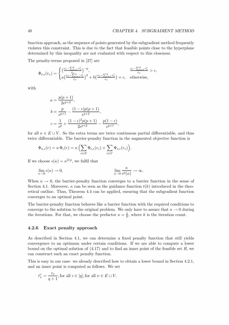
48 CHAPTER 4. SUBGRADIENT METHOD
function approach, as the sequence of points generated by the subgradient method frequentlyviolates this constraint. This is due to the fact that feasible points close to the hyperplanedetermined by this inequality are not evaluated with respect to this closeness.
The penalty-terms proposed in [27] are
Φν,ǫ(rν) =
{
( cν−Pq
i=1riν
cν
)−p,
cν−Pq
i=1riν
cν> ǫ,
a( cν−
Pqi=1
riν
cν
)2+ b( cν−
Pqi=1
riν
cν
)
+ c, otherwise,
with
a =p(p + 1)
2ǫp+2,
b =p
ǫp+1− (1− ǫ)p(p + 1)
ǫp+2,
c =1
ǫp+
(1− ǫ)2p(p + 1)
2ǫp+2− p(1− ǫ)
ǫp+1,
for all ν ∈ E ∪ V . So the extra terms are twice continuous partial differentiable, and thustwice differentiable. The barrier-penalty function in the augmented objective function is
Φκ,ǫ(r) = κΦǫ(r) = κ(
∑
e∈E
Φe,ǫ(re) +∑
v∈V
Φv,ǫ(rv))
.
If we choose ǫ(κ) = κ2/p, we fulfil that
limκ→0
ǫ(κ)→ 0, limκ→0
κ
ǫp(κ)→∞.
When κ → 0, the barrier-penalty function converges to a barrier function in the sense ofSection 4.1. Moreover, κ can be seen as the guidance function t(k) introduced in the theo-retical outline. Thus, Theorem 4.4 can be applied, ensuring that the subgradient functionconverges to an optimal point.
The barrier-penalty function behaves like a barrier function with the required conditions toconverge to the solution to the original problem. We only have to assure that κ→ 0 duringthe iterations. For that, we choose the prefactor κ = 1
k , where k is the iteration count.
4.2.6 Exact penalty approach
As described in Section 4.1, we can determine a fixed penalty function that still yieldsconvergence to an optimum under certain conditions. If we are able to compute a lowerbound on the optimal solution of (4.17) and to find an inner point of the feasible set R, wecan construct such an exact penalty function.
This is easy in our case: we already described how to obtain a lower bound in Section 4.2.1,and an inner point is computed as follows. We set
riν =
cν
q + 1, for all i ∈ [q], for all ν ∈ E ∪ V.
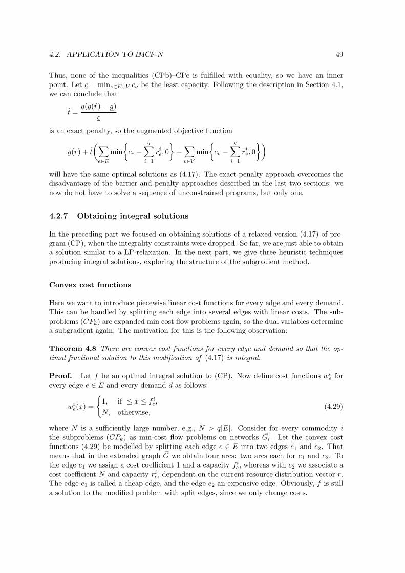
4.2. APPLICATION TO IMCF-N 49
Thus, none of the inequalities (CPb)–CPe is fulfilled with equality, so we have an innerpoint. Let c = minν∈E∪V cν be the least capacity. Following the description in Section 4.1,we can conclude that
t =q(g(r)− g)
c
is an exact penalty, so the augmented objective function
g(r) + t
(
∑
e∈E
min
{
ce −q∑
i=1
rie, 0
}
+∑
v∈V
min
{
cv −q∑
i=1
riv, 0
})
will have the same optimal solutions as (4.17). The exact penalty approach overcomes thedisadvantage of the barrier and penalty approaches described in the last two sections: wenow do not have to solve a sequence of unconstrained programs, but only one.
4.2.7 Obtaining integral solutions
In the preceding part we focused on obtaining solutions of a relaxed version (4.17) of pro-gram (CP), when the integrality constraints were dropped. So far, we are just able to obtaina solution similar to a LP-relaxation. In the next part, we give three heuristic techniquesproducing integral solutions, exploring the structure of the subgradient method.
Convex cost functions
Here we want to introduce piecewise linear cost functions for every edge and every demand.This can be handled by splitting each edge into several edges with linear costs. The sub-problems (CPk) are expanded min cost flow problems again, so the dual variables determinea subgradient again. The motivation for this is the following observation:
Theorem 4.8 There are convex cost functions for every edge and demand so that the op-timal fractional solution to this modification of (4.17) is integral.
Proof. Let f be an optimal integral solution to (CP). Now define cost functions wie for
every edge e ∈ E and every demand d as follows:
wie(x) =
{
1, if ≤ x ≤ f ie,
N, otherwise,(4.29)
where N is a sufficiently large number, e.g., N > q|E|. Consider for every commodity ithe subproblems (CPk) as min-cost flow problems on networks ~Gi. Let the convex costfunctions (4.29) be modelled by splitting each edge e ∈ E into two edges e1 and e2. Thatmeans that in the extended graph ~G we obtain four arcs: two arcs each for e1 and e2. Tothe edge e1 we assign a cost coefficient 1 and a capacity f i
e, whereas with e2 we associate acost coefficient N and capacity ri
e, dependent on the current resource distribution vector r.The edge e1 is called a cheap edge, and the edge e2 an expensive edge. Obviously, f is stilla solution to the modified problem with split edges, since we only change costs.
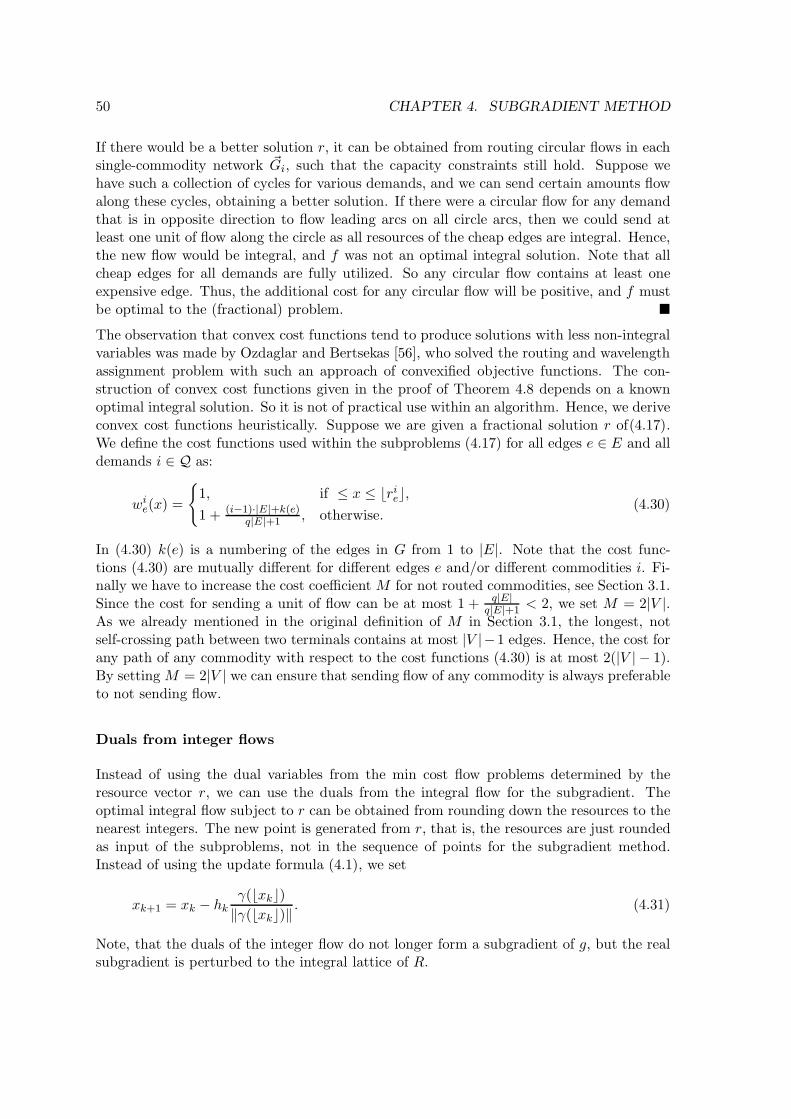
50 CHAPTER 4. SUBGRADIENT METHOD
If there would be a better solution r, it can be obtained from routing circular flows in eachsingle-commodity network ~Gi, such that the capacity constraints still hold. Suppose wehave such a collection of cycles for various demands, and we can send certain amounts flowalong these cycles, obtaining a better solution. If there were a circular flow for any demandthat is in opposite direction to flow leading arcs on all circle arcs, then we could send atleast one unit of flow along the circle as all resources of the cheap edges are integral. Hence,the new flow would be integral, and f was not an optimal integral solution. Note that allcheap edges for all demands are fully utilized. So any circular flow contains at least oneexpensive edge. Thus, the additional cost for any circular flow will be positive, and f mustbe optimal to the (fractional) problem. �The observation that convex cost functions tend to produce solutions with less non-integralvariables was made by Ozdaglar and Bertsekas [56], who solved the routing and wavelengthassignment problem with such an approach of convexified objective functions. The con-struction of convex cost functions given in the proof of Theorem 4.8 depends on a knownoptimal integral solution. So it is not of practical use within an algorithm. Hence, we deriveconvex cost functions heuristically. Suppose we are given a fractional solution r of(4.17).We define the cost functions used within the subproblems (4.17) for all edges e ∈ E and alldemands i ∈ Q as:
wie(x) =
{
1, if ≤ x ≤ ⌊rie⌋,
1 + (i−1)·|E|+k(e)q|E|+1 , otherwise.
(4.30)
In (4.30) k(e) is a numbering of the edges in G from 1 to |E|. Note that the cost func-tions (4.30) are mutually different for different edges e and/or different commodities i. Fi-nally we have to increase the cost coefficient M for not routed commodities, see Section 3.1.Since the cost for sending a unit of flow can be at most 1 + q|E|
q|E|+1 < 2, we set M = 2|V |.As we already mentioned in the original definition of M in Section 3.1, the longest, notself-crossing path between two terminals contains at most |V |−1 edges. Hence, the cost forany path of any commodity with respect to the cost functions (4.30) is at most 2(|V | − 1).By setting M = 2|V | we can ensure that sending flow of any commodity is always preferableto not sending flow.
Duals from integer flows
Instead of using the dual variables from the min cost flow problems determined by theresource vector r, we can use the duals from the integral flow for the subgradient. Theoptimal integral flow subject to r can be obtained from rounding down the resources to thenearest integers. The new point is generated from r, that is, the resources are just roundedas input of the subproblems, not in the sequence of points for the subgradient method.Instead of using the update formula (4.1), we set
xk+1 = xk − hkγ(⌊xk⌋)‖γ(⌊xk⌋)‖
. (4.31)
Note, that the duals of the integer flow do not longer form a subgradient of g, but the realsubgradient is perturbed to the integral lattice of R.
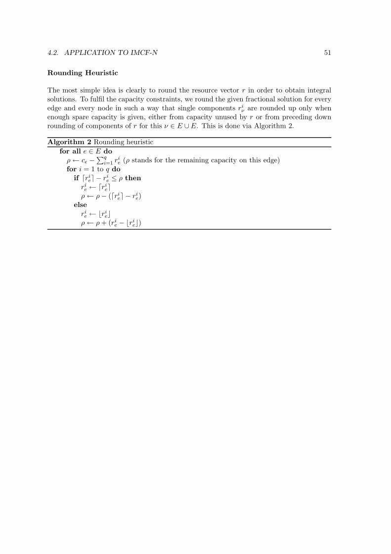
4.2. APPLICATION TO IMCF-N 51
Rounding Heuristic
The most simple idea is clearly to round the resource vector r in order to obtain integralsolutions. To fulfil the capacity constraints, we round the given fractional solution for everyedge and every node in such a way that single components ri
ν are rounded up only whenenough spare capacity is given, either from capacity unused by r or from preceding downrounding of components of r for this ν ∈ E ∪ E. This is done via Algorithm 2.
Algorithm 2 Rounding heuristic
for all e ∈ E doρ← ce −
∑qi=1 ri
e (ρ stands for the remaining capacity on this edge)for i = 1 to q do
if ⌈rie⌉ − ri
e ≤ ρ thenrie ← ⌈ri
e⌉ρ← ρ− (⌈ri
e⌉ − rie)
elserie ← ⌊ri
e⌋ρ← ρ + (ri
e − ⌊rie⌋)

52 CHAPTER 4. SUBGRADIENT METHOD
Chapter 5
Branch-and-cut method
In this chapter we focus on a solution technique for integer linear programs, known asthe branch-and-cut method. We use it to solve our problem via the formulation (RDF),presented in Section 3.2.3. As in the previous chapter, we first outline the general idea ofthe method, and then describe its application to our problem.
5.1 Theoretical framework
Branch-and-cut is a combination of two solution approaches: cutting plane method andbranch-and-bound method. We first describe these two approaches separately, and thentheir combination.
5.1.1 Cutting plane method
The cutting plane method is known since the late 1950’s, when Gomory [28, 29] used it tostrengthen LP-relaxations of integer and mixed integer programs. It has become a powerfultool in solving many combinatorial optimization problems and, more general, mixed integerprograms.
Suppose we are given a linear program with n variables and m linear inequalities:
min cT x, (5.1a)
Ax ≤b, with A ∈ Rm×n, b ∈ Rm, c ∈ Rn. (5.1b)
Note that every linear program can be transformed to a representation (5.1). The feasibleset of (5.1) is a polyhedron denoted by
P[m] = {x ∈ Rn : Ax ≤ b}. (5.2)
Assume, that m is very large, i.e., passing all inequalities into a LP-solver is not possible,or not desirable due to the expected solution time. From polyhedral theory, we know thateach vertex of the polyhedron P[m] can be described by the intersection of n hyperplanes,
53
54 CHAPTER 5. BRANCH-AND-CUT METHOD
arising from inequalities ATi x ≤ bi satisfied at equality. Here, Ai denotes the ith row of the
constraint matrix A in (5.1). Thus, we would need only n inequalities for the descriptionof an optimal vertex of the polyhedron, too. So, the basic idea of the cutting plane methodis to solve a reduced formulation of the linear program (5.1) first. For that, let I ⊂ [m] bea row index set of matrix A, we start by solving the reduced formulation
min cT x, (5.3a)
AIx ≤bI . (5.3b)
Then we check whether the optimal solution of (5.3), x∗I , violates inequalities AT
k x∗I ≤ bk
not yet included in the formulation (5.3), i.e., k ∈ [m] \ I. The process of recognizing suchviolated inequalities is called separation. If we find violated inequalities, they (or only someof them) are included in the reduced formulation, i.e.,
I ′ = I ∪ {k ∈ [m] : ATk x∗
I > bk}. (5.4)
The reduced formulation (5.3) is reoptimized with the new extended row index set I ′. Thewhole process
1. Optimizing the reduced formulation
2. Separation of violated inequalities
3. Extending the reduced formulation to violated inequalities
is iterated until the separation fails. Clearly, we will iterate only a finite number of times:in each iteration, at least one inequality is added to the reduced formulation. So at thelatest we stop if all inequalities of the original formulation (5.1) are included in the reducedformulation. By adding violated inequalities step by step we hope to consider only inequal-ities that are more likely to be used for an overall optimal solution of (5.1). Hence, wepossibly finish the iteration with far less inequalities than in (5.1).
From a polyhedral point of view, the added inequalities serve as cutting planes. To seethis, consider a polyhedron PI arising in the iteration, and the optimal solution x∗
I of theassociated reduced program (5.3) with respect to row index set I. By adding violatedinequalities by (5.4) we obtain a new polyhedron PI′ , that does not contain x∗
I . Hence,the hyperplanes associated with the added inequalities “cut off” the point x∗
I from thepolyhedron.
A typical reason for linear programs containing a large number of inequalities is that thelinear program arises as a LP-relaxation of a mixed integer program. Consider the mixedinteger program
min cT x + dT y, (5.5a)
Ax + By ≤ b, (5.5b)
x ∈ Rn1, (5.5c)
y ∈ Zn2. (5.5d)
5.1. THEORETICAL FRAMEWORK 55
Then (5.5) can be solved as a linear program with feasible set
PMIP = conv{(x, y) ∈ Rn1 × Zn2 : Ax + By ≤ b}. (5.6)
Clearly, PMIP is a polyhedron and can be described by a set of inequalities. These inequal-ities are usually not all known in advance. So (5.5) can be solved with a cutting planealgorithm, starting with the LP-relaxation of (5.5). If the optimal solution (x∗, y∗) of theLP-relaxation yields non-integral variables y∗i , additional inequalities that are valid for (5.6)must be provided. There are several known methods to generate such valid inequalities fromsolutions that do not satisfy all integrality constraints in (5.5). Among such methods areGomory-cuts, General upper bound-cuts, Flow cover-cuts, and Disjunctive cuts, to namejust a few. For a survey on these methods see, e.g., [69].
Note, that the cutting plane method relies on the solver’s ability to fast reoptimize a linearprogram after new inequalities are added. If the sequence of relaxed linear programs (5.3)had to be solved from scratch in each iteration, the cutting plane method would loose muchof its advantages. Fortunately, the ability of easy reoptimizing is given, e.g., when usingthe dual simplex method, see [59].
5.1.2 Branch-and-bound
Here, we turn to the branch-and-bound method. We first state the basic principle, andthen turn to its application to mixed integer programs. This method was first described byLand and Doig [45] and was refined in the following by Little et. al. [47] (who founded thename of the method), Dakin [16], and Balas [6], to name just a few. For a detailed surveysee [53].
The main idea can be seen as a divide-and-conquer principle: suppose we are given aminimization problem with feasible set S and objective function g, and
z∗ = minx∈S
g(x) (5.7)
is its optimal solution value. Furthermore, let the feasible set be decomposed in a finitenumber K of smaller sets, S = S1 ∪ · · · ∪ SK , with optima
zk = minx∈Sk
g(x), ∀k ∈ [K]. (5.8)
Then clearly z∗ = mink∈[K] zk. If the subproblems (5.8) are easier to solve than the originalproblem(5.7), the decomposition can be advantageous. The decomposition is the “branch-ing” part of the branch-and-bound method. It is improved by the “bounding” part, we de-scribe next. Let zk, zk be (local) lower and upper bounds on zk, for each subproblem (5.8).Then z = mink∈[K] zk is a (global) lower bound on z∗, and z = mink∈[K] zk is a (global)upper bound on z∗. If for some subproblem (5.8) we get zk ≥ z, we do not need considerthis subproblem any further, as it could not yield a better solution than the solutions foundin the remaining subproblems. Neglecting a subproblem because of its lower bound andthe overall upper bound is called pruning by bound. It might be possible that some of thesubproblems (5.8) are infeasible, i.e., if some Sk are empty. Such a subproblem with proveninfeasibility can also be dismissed, this operation is called pruning by infeasibility. Finally,
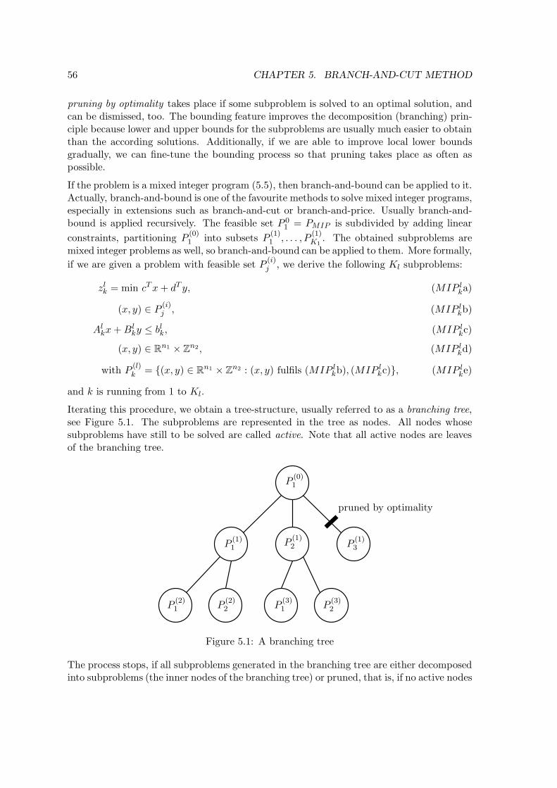
56 CHAPTER 5. BRANCH-AND-CUT METHOD
pruning by optimality takes place if some subproblem is solved to an optimal solution, andcan be dismissed, too. The bounding feature improves the decomposition (branching) prin-ciple because lower and upper bounds for the subproblems are usually much easier to obtainthan the according solutions. Additionally, if we are able to improve local lower boundsgradually, we can fine-tune the bounding process so that pruning takes place as often aspossible.
If the problem is a mixed integer program (5.5), then branch-and-bound can be applied to it.Actually, branch-and-bound is one of the favourite methods to solve mixed integer programs,especially in extensions such as branch-and-cut or branch-and-price. Usually branch-and-bound is applied recursively. The feasible set P 0
1 = PMIP is subdivided by adding linear
constraints, partitioning P(0)1 into subsets P
(1)1 , . . . , P
(1)K1
. The obtained subproblems aremixed integer problems as well, so branch-and-bound can be applied to them. More formally,
if we are given a problem with feasible set P(i)j , we derive the following Kl subproblems:
zlk = min cT x + dT y, (MIP l
ka)
(x, y) ∈ P(i)j , (MIP l
kb)
Alkx + Bl
ky ≤ blk, (MIP l
kc)
(x, y) ∈ Rn1 × Zn2, (MIP lkd)
with P(l)k = {(x, y) ∈ Rn1 × Zn2 : (x, y) fulfils (MIP l
kb), (MIP lkc)}, (MIP l
ke)
and k is running from 1 to Kl.
Iterating this procedure, we obtain a tree-structure, usually referred to as a branching tree,see Figure 5.1. The subproblems are represented in the tree as nodes. All nodes whosesubproblems have still to be solved are called active. Note that all active nodes are leavesof the branching tree.
pruned by optimality
P(0)1
P(1)1
P(1)2 P
(1)3
P(2)1 P
(2)2 P
(3)1 P
(3)2
Figure 5.1: A branching tree
The process stops, if all subproblems generated in the branching tree are either decomposedinto subproblems (the inner nodes of the branching tree) or pruned, that is, if no active nodes
5.1. THEORETICAL FRAMEWORK 57
are left. The overall optimal solution of the original problem is then the best (minimal)solution among the solutions of the subproblems. If no such solution was found, the originalproblem is infeasible.
To solve the mixed integer problem this way becomes similar to a complete enumerationof all of the integral variables, if the branching tree is fully explored. Such a completeenumeration yield an exponential number of subproblems to solve. The bounding processis the key tool to prevent the number of subproblems to grow too fast. Note however, thatbounding can not guarantee to obtain only a polynomial number of subproblems.
How can lower and upper bounds be derived for the subproblems? Clearly, the LP-relaxationof any subproblem yield a local lower bound zl
k of a subproblem MIP lk. On the other hand,
any feasible point of PMIP yields an upper bound for the subproblem’s solution. Suchfeasible points are derived by a heuristic, or occur as optimal solutions of subproblems.Clearly, tight lower and upper bounds will shorten the branch-and-bound procedure, asmore subproblems are likely to be pruned.
Several parts of the branch-and-bound procedure are still to be specified in more detail:
• Branching rule
We already described the general branching in (MIP lk). The open question is how
the branching constraints(MIP lkc) are derived. For that, let aT x be a linear form
with integral coefficients, and let {b1, . . . , bL} be the set of all integral values thataT y can attain in P i
j . Then we can derive Kl subproblems MIP l1, . . . , P
lLl
by adding
constraint aT y = bi to P ij , for all i ∈ [Ll]. Then the P l
k are clearly disjunct, and all
integral points feasible for P ij are feasible for some P l
k.
As the running time of most LP-solvers is very sensitive to the number of non-zerocoefficients of the constraints, a good choice for a is a unit vector. That means, thatwe actually branch on a single variable yt, obtaining subproblems with additionalconstraints yt = bi, for i ∈ [Kl]. Another advantage of branching on single variables isthat the admissible values b1, . . . , bKl
are usually easy to compute. Moreover, fixing avariable yt with a constraint yt = bi decreases the subproblem’s size, as the variableis no longer present in the subproblem, but can be replaced by the constant bi.
If the number L of admissible values bi is large, the scheme with adding equalityconstraints to the subproblems lead to a large number of subproblems. So a twoway branching rule is possibly preferable. A two way branching rule produces onlytwo subproblems Pi, Pj by adding constraints aT x ≤ b, aT x ≥ b + 1 to Pi, Pj ,respectively. Here, b ∈ {b1, . . . , bL} is an integer carefully chosen dependent on thefractional solution of Pk.
The most widely used branching rule is a two way branching rule on single variables.That means, that in subproblem MIP i
j an integral variable yt is selected and an as-
sociated branching value β /∈ Z. Two subproblems MIP l1 and MIP l
2 are created byadding the restrictions yt ≤ ⌊β⌋ and yt ≥ ⌈β⌉, respectively. A two way branchingrule has the advantage that only two new problems arise in the branching tree. More-over, the added constraints are simple in the sense of non-zero coefficients. SometimesLP-solvers can handle bounds on variables in a special manner, decreasing the com-
58 CHAPTER 5. BRANCH-AND-CUT METHOD
putational effort even more. Finally, branching on a fractional variable is likely toforce this variable to an integer value.
When applying this two way branching rule, we still have to decide on which variablewe want to branch. The best idea is usually to branch on an integral variable that hasa fractional value in the optimal fractional solution of P i
j . As the optimum zlk of the
LP-relaxation of MIP ij is neither feasible for MIP l
1 nor for MIP l2, we can hope that
the optima of MIP l1 and MIP l
2 are strictly greater than zlk, thus possibly improving
the overall lower bound z. Again, there might be several possibilities for branchingvariables in Pk. Taking the mentioned improvement of the lower bound into account,typical choices are either to choose branching variables with large cost coefficients, orvariables with small reduced costs, or variables whose fractional value part is closestto 0.5.
Branching rules are shown to have a great impact on the branching tree’s size, andthus on the running time of the solution process. The decision which branching ruleshould be used depends on the program to be solved, and no general preferable rulecan be given.
• Node selection
The sequence in which the subproblems should be examined is another importantparameter of the branch-and-bound process. Again, a robust node selection ruleworking best for all problems is not known. So, we have to determine a good rule foreach problem on its own.
Choosing the “right” subproblem will yield tighter lower or upper bounds. Thus, atypical procedure is choosing a branching node with a least local lower bound, as thenew arising subproblems are likely to provide better bounds. Note that the least locallower bound determines the global local bound. Another approach is to choose thenode with best upper bound, as better or even optimal solutions are to find moreprobably in the neighbourhood of already known good solutions. Finally, we mentionthe diving rule. This rule selects a node that is deepest in the search tree. Sucha node has underrun most branching decisions among all yet active nodes, so theselected node represents a most restricted subproblem. Hence, we can hope to eitherobtain a good lower bound from this node, or to prune the node.
• Heuristics
Obtaining good upper bounds decreases the number of search tree nodes considerably.Unfortunately, a general scheme for deriving good feasible solutions is not given.General purpose solvers try to round fractional variables in some constraint dependentsequence. However, a problem specific heuristic is usually preferable.
5.1.3 Branch-and-cut
We next turn to the question how cutting plane method and branch-and-bound can becombined. The general scheme of branch-and-cut is similar to the branch-and-bound schemedescribed above. We consider a branching tree as well, but in contrast to simple branch-and-bound cutting planes can be generated at every node of the branching tree. So, in each
5.2. APPLICATION TO IMCF-N 59
node a cutting plane method takes place. The only difference is that a subproblem needsnot to be solved to integer optimality with the cutting plane method, as we can chooseto branch on this subproblem. In case of combinatorial cutting planes, we must be carefulwhen deriving upper bounds. A heuristic producing such upper bounds has to consider thatthere can be valid inequalities that are not yet part of the description, but are necessaryfor a correct description. Thus, a point satisfying all constraints at some branching nodemight not be feasible for the original problem. The point rather has to be checked whetheror not it fulfils all restrictions that are part of the problem. Only if it does so it can be usedfor an upper bound.
5.2 Application to IMCF-N
We next describe how branch-and-cut can be applied to our problem IMCF-N, based on theformulation (RDF), as given in Section 3.2.3. First we motivate why we use branch-and-cut,and specify the components of the method introduced in Section 5.1. As mentioned, wehave to decide on a branching rule, a node selection scheme, a heuristic for upper bounds,and on a separation method for cutting planes.
The reason for applying branch-and-cut to formulation (RDF) is twofold. First, the formula-tion contains an exponential number of inequalities arising from the general cuts in (RDFd).In general, the number of general cuts in a graph can be exponential in the number of edgesand nodes of the graph. So we can not include all general cut constraints, since the timeneeded to solve the linear programs occurring in a branch-and-bound tree would be toolarge. Moreover, since we deal with q(|V | + |E| + 1) variables in formulation (RDF), onlyq(|V |+ |E|+ 1) inequalities of the formulation can be linearly independent. Hence, most ofthe general cut constraints are redundant, and we consider them only as demanded, i.e., ifthey are violated during the solution process. The second reason for using branch-and-cutis that we deal with an integer program, and branch-and-cut is one of the most successfulsolution methods for integer programs.
The initial relaxation of formulation (RDF) is a LP-relaxation, where the capacity con-straints (RDFb), (RDFc), and the diversification constraints (RDFe), (RDFf) are included.Additionally, some of the general cut constraints (RDFd) were included as well by the fol-lowing construction. For each demand k ∈ Q independently, we start with all resourceszero, i.e., rk
ν = 0, for all ν ∈ V ∪ E. With the separating routine described in Section 5.2.4we generated minimal general sk-tk-cuts as long as no such cut could be found with capacityless than dk. Once a cut was found, one edge or node in the cut was assigned a resourcedk. Thus, no cut can occur twice.
5.2.1 Branching rule
We decide to use a two way branching scheme on single variables as described in Section 5.1.The branching variables are chosen in order of decreasing costs. Thus, the artificial variablesak describing the amount of flow not routed for demand k are chosen first, if they are notintegral. As all variables ak have the same cost coefficient, we still have to decide which
60 CHAPTER 5. BRANCH-AND-CUT METHOD
of these variables to choose for branching, if more than one of them is not integral in asolution of a intermediate relaxation. In that case, we choose the most fractional variable,i.e., the variable ak whose fractional part is closest to 0.5. If all variables ak are integral,the edge resource variables rk
e are chosen next as possible branching variables. Finally, thenode resource variables rk
v are considered. For the resource variables rke and rk
v the sametie-breaking rule is applied as for the ak. That is, if more than one has a non-integral value,we choose the most fractional. We choose this branching order to obtain rapidly increasinglower bounds, since a change of a variable with high associated costs has more impact onthe objective value. By this, we aim to keep the branching tree’s size as small as possible.
5.2.2 Node selection
Computational experiments showed that even in the case of small gaps between lower andupper bound a large number of nodes has to be considered. Thus, pruning nodes is verydesirable. By testing some standard rules we have decided to choose to branch on a nodewith a local lower bound equal to the global local bound.
5.2.3 Heuristics
To obtain upper bounds we used the built-in heuristic of the MIP-solver CPLEX. Thisheuristic yields already good upper bounds. Thus, a problem specific heuristic can notimprove the upper bound that much. Due to the complexity results given in Section 2.4.1it would be difficult to develop a combinatorial heuristic anyway.
5.2.4 Cutting planes
We next describe how cutting planes were involved. As already mentioned, the numberof general cuts in formulation (RDF) can be very large. So we decided to put only fewgeneral cuts into the initial formulation, and we added more of them only when they wererecognized to be violated.
The separation procedure works as follows. Suppose we are given a point (r∗, a∗), that isconsidered optimal in the current relaxation, at some node of the branching tree. So foreach k ∈ Q, we have resources r∗ke for all edges e ∈ E, and r∗kv for all vertices v ∈ V . Thenwe are able to compute a minimal general sk-tk-cut for demand k. This can be done via anystandard max-flow or min-cut procedure. We decided to use a network simplex procedure,working on the extended graph ~G as described in Section 3.2.4. Once we have found aminimal general sk-tk-cut, we check whether this cut has capacity at least dk − ak. If not,we have found a violated inequality to be added as a cutting plane.
When given a point (r, a), we decided to check for cutting planes for all demands, tofasten computation. So we can add at most q cutting planes at once, avoiding intermediatereoptimization.
The general cuts present in the initial formulation are generated as follows.
5.2. APPLICATION TO IMCF-N 61
The number of initial cuts derived like this was substantial, compared to the number of cutsgenerated at all. Although no guarantee can be given that the initial cuts are good in thesense of being inevitable in an optimal solution, they turned out to be useful in speedingup the solution process.
Details of the influence of the methods outlined on the solution process are described inChapter 6.

62 CHAPTER 5. BRANCH-AND-CUT METHOD
Chapter 6
Computational results
In this chapter we describe the application of the methods outlined in the Chapters 4and 5. First, we give some implementation details and mention the software incorporatedin Section 6.1. In Section 6.2 we describe the test instances we used for the comparison ofthe methods. Finally, we report on the obtained results in Section 6.3, and analyse them.
6.1 Implementation
We implemented the methods described in the Sections 4.2 and 5.2 in C++ using the ANSIStandard Template Library. Our implementation was built on top of the Optical NetworkDesign (OND) project software by Koster and Zymolka, see [71]. As the implementation ofthe min cost flow solver the software MCF by Lobel [49] was used through the MCFClassinterface by Frangioni [20]. The branch-and-cut method was developed with CPLEX 7.5and Concert Technology 1.2 [37, 36].
6.2 Test instances
Unfortunately, there are no instances for IMCF-N publicly available to compare our resultswith other researcher’s results. A collection of instances of the fractional multicommodityflow problem is provided in [21], together with some computational results from variousmodels and implementations. These instances are not suited for our purposes due to theircharacteristics: they contain large supply graphs, or very dense supply graphs, or very fewdemands. So we have chosen to build own test instances, inspired by the instance generatordescribed in [11].
Our instance generator works as follows. First of all, we have to provide the following inputdata:
• the number of vertices |V | in the supply graph,
• a density parameter δ for the supply graph,
63
64 CHAPTER 6. COMPUTATIONAL RESULTS
• the number of demands q,
• the diversification parameter ρ.
Then the instance generator computes a random position in the plane for every vertex ofthe supply graph. These positions are uniformly distributed in the square [0, 100]× [0, 100].Afterwards a set Epot of δ(|V | − 1) of potential supply edges is generated by δ minimumspanning tree computations in the following way. We start with the complete graph G =(V, E). To each edge vw ∈ E we assign a weight that is the Euclidean distance betweenv and w. In the beginning let Epot = ∅. In each of δ iterations, we compute a minimumspanning tree of G with respect to the edge weights. Let Et be the edge set of the spanningtree. We set E ← E\Et, Epot ← Epot∪Et, and the next iteration follows. This constructionyields a set of potential supply edges similar to real world instances. Since costs of opticalfibers are length dependent, supply graphs are rather sparse, and short edges are preferredto long edges.
After constructing the potential supply edges, the demands are computed. For that, qterminal pairs are randomly chosen, uniformly distributed among all vertex pairs vw ∈V ×V . The according demand values are randomly chosen integers from the interval [1, 15].We provide the same diversification parameter ρ for all demands.
To obtain instances that are close to real world instances, the dimensioning of the networkis carried out by the tool DISCNET by Wessaly [68] and the preprocessing features of theOND software. The input of this tool is a set of potential vertices and edges that can beestablished as supply vertices and supply edges. Furthermore, demands must be specified,i.e., the demand’s terminals, its value, and diversification parameter. Finally, the installablehardware must be given, as described in Chapter 2. For that, optical fibers, WDM systems,and OXCs are specified with their routing capacity (in terms of lightpaths) and costs. Tothe WDM systems we assigned a capacity of 10 channels, and we provided 2 types of OXCswith capacity for 2 and 5 lightpaths, respectively.
DISCNET computes from this input a dimensioning of the optical network, minimizing theoverall costs of installed hardware. It is guaranteed that all demands can be fully routedwith respect to its diversification parameter, but the flow can be fractional. However, thedimensioning is provided in integral units of the routing capacity of the specified hardware.
By applying DISCNET we obtain a supply graph that is tight dimensioned in the sensethat most demands can be fully satisfied by integral routings, while many supply edgesand nodes are fully utilized. The instances obtained this way are described as having tightcapacities in Table 1. To explore the behaviour of our solution approaches in more detail,we also derive high and low dimensioned instances from the tight dimensioned ones. Thehigh dimensioned instances have twice the capacity on every edge and vertex as the tightdimensioned instances, while in the low dimensioned instances it is half the capacity. Itis likely that the high dimensioned instances have enough edge and vertex capacities tosatisfy all demands, and that the according capacity bounds are not the main influence ofthe optimal solution value. So we can observe the performance of the solution methods if lessinterference between the commodities takes place. On the other hand, the low dimensionedinstances shall give an insight into how the solution methods perform if not enough capacityis given to route all commodities.
6.3. RESULTS 65
The instances created this way differ in four characteristics:
• The supply graph size ranges from 10 vertices to 76 vertices, while the supply graphdensity pG = 2|E|
|V |(|V |−1) ranges from 0.04 to 0.58. The graph density depends on theparameter δ used in the initial construction of the instances. By the instance con-struction the relation pG ≤ 2δ
|V | holds. Due to the dimensioning process of DISCNETthat determines which potential supply edges are realized, the same δ parameter canlead to a different number of actual supply edges and graph densities pG.
• The number of demands ranges from 15 to 150, or as expressed with the demandgraph density pH = 2q
|T |(|T |−1) , pH ranges from 0.01 to 0.89. Recall that T is the setof demand terminals, i.e., the set of vertices of the demand graph.
• The diversification parameter used are 0.25, 0.5, and 0.75. Note that a diversificationparameter 0.25 requires that at least four vertex-disjoint paths between the terminalvertices of each demand exist.
• The provided capacities range roughly from half of the capacities needed to route allcommodities to twice the capacity needed to route all commodities.
The details of the single instances we used can be seen in Table 1. The names of the in-stances contain the parameters that are used when constructing the instances. For example,N20 G3 H100 D75 h stands for 10 vertices, a density parameter δ = 3, 100 commodities, adiversification parameter ρ = 0.75 for all demands, and finally a high dimensioned instance.
6.3 Results
In this section we first describe the computational results of the subgradient method appliedto formulation (CP). We characterize the best parameters of the subgradient method, foreach variant of the method. By choosing the best parameters and the best variants, wecompare the results for the three heuristics described in Section 4.2.7. Then we give theresults obtained by the branch-and-cut method for formulation (RDF). Finally, we comparethe results of both methods to the benchmark results obtained with formulation (EFF).
6.3.1 Results of the subgradient method
In Section 4.2 we outlined that the subgradient method is suitable to be applied to theformulation (CP). We presented six variants of the subgradient methods that differ in theway the constraints (CPb)–(CPe) are treated. In a first step, we compare these variantsby applying only the rounding heuristic described in Section 4.2.7. For all test runs we seta running time of 60 seconds. Experiments have shown that the quality of the solutionsdoes not improve significantly if more running time is given to the methods. Comparingall variants by the same running time, i.e., instead of comparing them by the number ofiterations, results from the heuristic character of the subgradient method. Since a heuristicis meant to be applied several times during an exact solution approach, the main issue isits running time.
66 CHAPTER 6. COMPUTATIONAL RESULTS
We use the Crowder adaption scheme, see Section 4.1, to extract the best variant of thesubgradient method. We extensively tested all variants to find an appropriate initial valuefor λ1 used in the step length computation, see Section 4.2.1. It turns out that a carefuladjustment of λ1 is essential. This can also be seen in Table 3, where the best values for λ1
for the different subgradient adjustment rules are listed. These results depict that the mostsuccessful values for λ1 differ substantially among the instances. The integral solutions areproduced by the rounding heuristic described in Section 4.2.7.
The results for the different constraint handling variants are given in Table 2. The qualityof the solution is measured in per cent, where the optimal solution or best lower boundis used as a reference. This reference value is taken from the branch-and-cut method foreither formulation (EFF) or formulation (RDF), cf. Section 6.3.2. It is more reliable thanthe lower bound computed by the subgradient method itself, since the quality of the lowerbound of the subgradient method varies strongly among the instances.
We make the following observations for the variants of the subgradient method:
• First of all, the projection method PROJ works best on all instances, followed bythe variation PROJ=. With dramatical gap the penalty method, the barrier-penaltymethod, the exact penalty method, and the barrier method follow in this order. Thereason for that is that the four penalizing methods yield large subgradients due to thepenalty terms in the augmented objective function.
• As expected, the solution quality decreases with increasing instance size. Especiallythe number of commodities has a large impact.
• The instances with high and low capacities are approximated best by all variants,while the tightly dimensioned instances are rather hard to approximate. This hardnessresults from the fact that in the tightly dimensioned instances usually all demands canbe fully satisfied in an optimal solution. By the subgradient method’s approximationusually a fraction of the demands can not be routed, and in that case the high costcoefficient for not routed demands increases the solution value fast.
Taking into account the above results we decide to use the projection variant PROJ through-out the following considerations. We next examine which subgradient adjustment ruleshould be used. In Chapter 4 we introduced the Crowder rule, the Camerini-Fratta-Maffioli(CFM) rule, and the modified Camerini-Fratta-Maffioli (mCFM) rule. We apply these rulestogether with the projection method PROJ, and again test for the best λ1 value. The re-sults can be seen in Table 3. In this table the results of the Crowder rule as applied toobtain the results of Table 2 are restated for comparison. We observe:
• The modified Camerini-Fratta-Maffioli rule and the Crowder rule work best. Thesimple Camerini-Fratta-Maffioli rule never yields the best result.
• The initial values λ1 differ substantially for different instances and different subgradi-ent adaption rules. Choosing other values for λ1 as presented in the table can lead toa dramatic loss of solution quality, even a divergent behaviour of the method occurs.
6.3. RESULTS 67
Finally we turn to the two heuristics for obtaining integral solutions, the convex cost heuris-tic and the integral flow subgradient heuristic as outlined in Section 4.2.7. Both heuristicsare combined with the rounding heuristic, since the first two mentioned heuristics do notensure to obtain an integral solution.
We decide to use the modified Camerini-Fratta-Maffioli rule for the comparison of theheuristics, since this rule proved to be successful in previous experiments. The results aregiven in Table 4, with a restatement of the results obtained without the heuristics fromTable 3. We observe:
• Both heuristics improve the solution quality compared to the results without theheuristic. However, the improvement is not substantial.
• Comparing the two heuristics, none of them is superior to the other. The convex costheuristic does less iterations due to the more complicated subproblems (CPk). Recallfrom Section 4.2.7 that for the convex cost heuristic each of the subproblems has twicethe arcs as in the integral flow subgradient heuristic, since the convex cost functionsare modelled by split edges. On the other hand, the heuristic using subgradientdirections derived by the integral flows lacks to reach integral points due to the steplengths used. Experiments with longer computation time does not yield better results.
By the results presented in this section we conclude that the subgradient method workswell for instances with high and low capacity. The most interesting instances however, i.e.,the tight dimensioned instances that refer to the application presented in Chapter 2, yieldunsatisfying results.
6.3.2 Results of the branch-and-cut method
We apply the branch-and-cut method to formulation (RDF) as described in Section 5.2.The running time for each instance was bounded to one hour. The results of the methodare presented in Table 5. The table lists the following details:
• Row GAP shows the gap between the best solution found and the lower bound of thebranch-and-cut method in per cent. A gap of 0.00 means that the according instancewas solved to optimality.
• Row TIME lists the time needed by the branch-and-cut method, rounded to seconds.This includes the time for the separation of the general cut inequalities, the time forthe MIP-solver, and the time for intermediate output, but not the time for readingthe data and constructing the initial data structures.
• Row INIT CUTS gives the number of initial cuts included in the first relaxation.
• Row CUTS shows the number of general cut inequalities generated in the wholeprocess, including the initial cuts.
• Row NODES lists the number of branching nodes that were generated in the branchingtree.
68 CHAPTER 6. COMPUTATIONAL RESULTS
Examining the obtained results we observe that 24 of the 33 instances are solved to op-timality, while for nine instances solutions within a gap of less than 0.42% are found. Incontrast to the results of the subgradient method, the low dimensioned instances turn outto be most difficult for the branch-and-cut approach. The number of branching nodes showsan interesting behaviour. The instances are either solved within few branching nodes orrequire a very large number of them. Note that the instances with most branching nodes areusually not solved to optimality, so even more nodes would be needed to reach optimality.
6.3.3 Comparison of the results
As mentioned in Chapter 3 we compare the results of the subgradient procedure for formula-tion (CP) and the results of the branch-and-cut method for formulation (RDF) with bench-mark results. Here, a branch-and-cut method applied to the standard formulation (EFF)serves as the benchmark. No parameter settings are made, i.e., node selection, branchingrule, and generation of cuts are left to the default behaviour of the MIP-solver. Again, atime bound of 3600 seconds is stipulated. In Table 6 the details of the obtained results aregiven. It contains the gap between the best solution found and the lower bound, measuredin per cent, the time needed for the computation, measured in seconds, and finally thenumber of rows in the formulation. The MIP-solver tries to aggregate formulation (EFF),and the number of rows given in Table 6 refers to after aggregation.
By the given results we conclude that the subgradient method together with the heuristicsto find integral solutions does not yield satisfying results. Only in special cases it providessolutions for formulation (CP) within reasonable tolerance. As already mentioned in Sec-tion 6.3.1, the most interesting instances are the tight dimensioned ones. Especially forthese instances the subgradient method is not competitive with the two branch-and-cutmethods. Additionally, the lack of a good lower bound in the subgradient method requiresthe use of other solution techniques to prove the quality of the obtained solutions.
Both branch-and-cut methods provide satisfying results for all instances. Especially thetight dimensioned instances, as of major interest, are solved quickly. The benchmark offormulation (EFF) is superior to the branch-and-cut method based on formulation (RDF).Comparing the number of generated cuts for (RDF) with the number of rows in (EFF) showsthat both formulations contain a similar number of constraints, except for low dimensionedinstances, where considerable more general cut inequalities are separated for (RDF). Thedifference in the running times is mainly due to the repeated resolving of the relaxations offormulation (RDF).
We also tested our implementation with real world instances provided to us by our projectpartners T-Nova. Due to a disclosure agreement we are not able to describe these instancesin detail. However, the instances given in Section 6.2 cover the main characteristics ofthe real world instances. Hence the results for them are similar to those results for the“artificial” instances.
Chapter 7
Conclusions
In this chapter we draw a conclusion on the results we obtained in this work. We firstjudge the capabilities of the subgradient approach. Then we summarize the results of thebranch-and-cut method. Both the heuristic and the exact approach are compared to thebenchmark formulation and its results. Finally, we give an outlook in Section 7.3.
7.1 Evaluation of the subgradient approach
The subgradient method produces feasible solutions for the test instances described inSection 6.2 within a gap of 1.2% to 157.3% to the best lower bound obtained by anymethod. This gap is unsatisfying large. Compared to the results of the two branch-and-cutmethods we must conclude that the subgradient method and the heuristics applied withinare unsuitable for our problem. The branch-and-cut methods produce better solutions,usually optimal solutions, in less time than the subgradient approach. Thus, there is noneed for the heuristic we suggested providing upper bounds.
The formulation (CP) (or its relaxation (4.17)) is not suitable to apply the subgradientmethod to produce lower bounds for formulations (EFF), (RDF). Since (CP) providesprimal solutions, primal in terms of formulation (RDF), the relaxation (4.17) must be solvedto proven approximated optimality to provide such a lower bound. But good approximationguarantees are beyond the capabilities of the subgradient method. However, the subgradientmethod might still be useful to solve a Lagrangian dual program to obtain lower bounds.
The results of the branch-and-cut method suggest that the difficulty of the integer routingproblem does not arises from bad upper and lower bounds, but from high degeneracy of theprograms due to many equivalent solutions. Thus, our subgradient approach is not neededto improve the performance of the exact solution approaches.
69
70 CHAPTER 7. CONCLUSIONS
7.2 Evaluation of the branch-and-cut approach
The branch-and-cut method described in Chapter 5 produces feasible solutions for all testinstances described in Section 6.2. The found solutions are mostly proven to be optimal,for a few instances a gap of up to 0.42% occurred.
It turned out that good lower and upper bounds were found quickly, but for some instancesit was difficult to obtain optimal solutions. The difficulties lead back to an enormousnumber of branching nodes. This is due to a large number of equivalent solutions. Theformulation (RDF) aimed to restrict the number of equivalent solutions, but any progresstoward this goal was nullified by the effort for separation of the general cut inequalities.
However, both branch-and-cut methods for the formulations (EFF), (RDF) offer a quickpossibility for solving the integer multicommodity flow problem at least approximately.Considering the underlying optical network design problem it turns out that obtaininggood solutions very fast is advantageous for the dimensioning task. If the overall designprocess is decomposed as described in Section 2.1.2 the dimensioning has to be repeateduntil a routing of all demands is possible. Both lower and upper bounds of the integerrouting problem contribute to this iteration. Lower bounds give necessary conditions forthe capacities to provide while upper bounds, i.e., feasible solutions prove sufficiency of theprovided capacities.
7.3 Outlook
To our opinion, a promising approach for future research is to review the formulations (EFF),(RDF) to decrease the degeneracy of these formulations. One possibility could be a dif-ferent objective function, where demands are rated differently. Another idea is to narrowthe set of feasible solutions by introducing additional constraints to the formulations. Bythat feasible solutions might be excluded as long as at least one optimal solution is stillcontained in the feasible set.
Another approach to achieve better performance of the branch-and-cut method is to focus onpolyhedral investigations. The dimensioning task of optical network design is often carriedout under use of Theorem 2.2. However, this applies only for fractional multicommodityflows. An extension to integer multicommodity flow would improve the approaches to thedimensioning problem and would yield deeper insight to the integer multicommodity flowproblem.
Zusammenfassung
Optische Netzwerke sind Netzwerke aus dem Telekommunikationsbereich, deren Vorteil inihren hohen Bandbreiten und Geschwindigkeiten liegt. Durch den technologischen Fort-schritt und die Moglichkeiten, die neuartige technische Komponenten bieten, wurden ma-thematische Losungsansatze vor neue Herausforderungen gestellt.
Diese Diplomarbeit entstand im Rahmen von Projekten des Konrad-Zuse-Instituts in Ko-operation mit zwei Industriepartnern. Die Projektarbeit verdeutlichte, dass die Probleme,die sich im Rahmen von optischen Netzwerken ergeben, mit den bisherigen Losungsmoglich-keiten nicht zufriedenstellend gelost werden konnen. Dies resultiert daraus, dass herkomm-liche Losungsansatze an der Komplexitat des Gesamtproblems scheitern.
Ziel dieser Arbeit ist es, Moglichkeiten und Losungsvorschlage fur ein spezielles Routing-problem zu entwickeln, dass im Rahmen der Gestaltung von optischen Netzwerken entsteht.Dieses Problem entsteht bei der Aufgabe, gegebene Kommunikationsanforderungen durchdie Verbindung der entsprechenden Terminals mit Hilfe von Pfaden zu erfullen.
Derartige Verbindungen werden im Rahmen von optischen Netzwerken mit Hilfe von Lichtwe-gen realisiert. Das Routingproblem besteht genau in dieser Realisierung ausreichenderLichtwege. Typischerweise konnen in solchen optischen Netzwerken die Lichtwege nichtbeliebig geteilt werden, sondern mussen als ganze Einheit bestehen bleiben. Daraus folgensystemimmanente Beschrankungen fur den mathematischen Losungsansatz.
Aufgrund des hohen wirtschaftlichen Aufwands sind die Routingkapazitaten eine knappeRessource, was das Problem zusatzlich erschwert. Es ist daher umso wichtiger, effektiveLosungswege fur das Routingproblem zu entwickeln.
Das Routingproblem ist bereits in anderen Bereichen und Anwendungen behandelt worden,jedoch ist der dieser Arbeit zugrunde liegende Losungsansatz neu. Wir haben uns furden so genannten ressourcenorientierten Zerlegungsansatz entschieden, da dieser besondersvielversprechend fur die spezifischen Anforderungen von optischen Netzwerken ist.
Zunachst stellen wir die grundlegenden Aspekte der optischen Netzwerke und die im Rah-men des Designprozesses entstehenden Probleme dar, womit die Schwierigkeit des zugrundeliegenden Problems verdeutlicht wird. Im Anschluß daran wird ein Modell und eine spezifis-che Formulierung entwickelt. Diese Formulierung wurde durch vorangegangene Forschungs-arbeiten und Untersuchungen in dieser Arbeit motiviert.
Ferner wurde ein Losungsansatz basierend auf der Subgradientenmethode entwickelt undanschließend durch heuristische Ansatze zur Behandlung der Ganzzahligkeitsbedingungen
71

72 ZUSAMMENFASSUNG
weiterentwickelt.
Es wurden verschiedene Varianten der einzelnen Aspekte der Subgradientenmethode ver-glichen. Weiterhin wurde ein exakter Losungsansatz, basierend auf dem Branch-and-CutVerfahren, entwickelt.
Mithilfe von Testinstanzen, die strukturell real existierenden optischen Netzwerken ahneln,werden die entwickelten Methoden schließlich getestet und bewertet.
Letztlich werden beide vorgestellten Losungsansatze und ihre Ergebnisse mit dem durcheine Standardformulierung erzielten Vergleichsansatz verglichen. Dieser Vergleichsansatzbasiert ebenfalls auf der Branch-and-Cut Methode.
Abschließend werden alle erzielten Ergebnisse verglichen und ausgewertet.
Abstract
Optical networks are structures arising in telecommunication. These optical networks pro-vide high speed and high bandwidth capabilities. Due to engineering progress and moderntechnical equipment new challenges appear to mathematical models and solution methods.
This thesis was inspired by two projects of the Konrad-Zuse-Zentrum with industrial part-ners. The project led to the realization that the problem of optical network design cannot be sufficiently solved by ordinary solution approaches which tackle the whole designproblem at once.
The aim of this work is to provide means and methods to solve a specific routing problemarising in the design process of optical networks. This problem evolves from the taskto provide connections between pairs of terminals dependent on a given communicationdemand. Such connections are realized via lightpaths in the optical network. The problemof establishing such lightpaths is known as a routing problem. An inherent characteristicof optical networks is that paths can not be split arbitrary but have to be provided in basicunits. This results in integrality constraints of the mathematical model.
Due to economic reasons capacities providing routing capabilities are scarce resources. Thisrequires sophisticated solution approaches for the routing problem. The routing problemhas arisen before in different areas and applications but was not yet approached from thepoint of our specification. This resource directed decomposition approach is chosen by ussince it is especially promising for the specific requirements of optical networks.
After surveying the basic aspects of optical networks and the problems arising in the designprocess we state the hardness of the problem under consideration. We extract a modelfor the routing problem and give a new formulation not yet studied. This formulation ismotivated by previous research and by considerations given in this work.
We develop an approach based on a subgradient method and extend it to handle the in-tegrality constraints heuristically. We test different variants of the single aspects of thesubgradient method. Furthermore, we tackle the problem by a branch-and-cut methodwhich leads us to an exact solution method. By providing test instances similar to realworld instances of optical networks we evaluate the developed methods. Both approachesare finally compared to a standard benchmark formulation, that is solved via a straightfor-ward branch-and-cut algorithm. Finally, the obtained results are analyzed and the methodsare evaluated.
73

74 ABSTRACT
Bibliography
[1] R. K. Ahuja, T. L. Magnanti, and J. B. Orlin. Network Flows: Theory, Algorithms,and Applications. Prentice Hall, New Jersey, 1993.
[2] Filipe Alvelos and J.M. Valerio de Carvalho. Solving the multicommodity flow prob-lem by branch-and-price. Technical report, Departamento de Producao e Sistemas,Universidade do Minho, Braga, Portugal, 2000.
[3] Arjang A. Assad. Models for rail transportation. Transportation Research, 14A:205–220, 1980.
[4] Y. Aumann and Y. Rabani. Approximate min-cut max-flow theorem and approxima-tion algorithm. SIAM Journal on Computing, 27:291–301, 1998.
[5] Mordecai Avriel. Nonlinear Programming: Analysis and Methods. Prentice Hall, En-glewood Cliffs, N.J., 1976.
[6] E. Balas. An additive algorithm for solving linear programs with zero-one variables.Operations Research, 13:517–546, 1965.
[7] Cynthia Barnhart, Christopher A. Hane, and Pamela H. Vance. Integer multicommod-ity flow problems. In Integer Programming and Combinatorial Optimization, Proceed-ings of the 5th International IPCO Conference, Vancouver, British Columbia, Canada,Lecture Notes in Computer Science, pages 59–71. Springer Verlag, 1996.
[8] Alok Baveja and Aranvind Srinivasan. Approximation algorithms for disjoint paths andrelated routing and packing problems. Mathematics of Operations Research, 25(2):255–280, 2000.
[9] Dimitri P. Bertsekas. Linear Network Optimization: Algorithms and Codes. MIT Press,Cambridge, 1991.
[10] P. Bruckner, J.L. Hurink, and T. Rolfes. Routing of railway carriages: A case study.Technical report, University of Twente, 1999.
[11] Lorenzo Brunetta, Michele Conforti, and Matteo Fischetti. A polyhedral approach toan integer multicommodity flow problem. Discrete Applied Mathematics, 101(1–3):13–36, 2000.
[12] P.M. Camerini, L. Fratta, and F. Maffioli. On improving relaxation methods by mod-ified gradient techniques. Mathematical Programming Study, 3:26–34, 1975.
75
76 BIBLIOGRAPHY
[13] Teodor Gabriel Crainic, Antonio Frangioni, and Bernard Gendron. Multicommoditycapacitated network design. In Telecommunications Network Planning, pages 1–19.Kluwer Academic Publisher, 1999.
[14] Teodor Gabriel Crainic, Antonio Frangioni, and Bernard Gendron. Bundle-based relax-ation methods for multicommodity capacitated fixed charge network design problems.Discrete Applied Mathematics, 112(1–3):73–99, 2001.
[15] H. Crowder. Computational Improvements for Subgradient Optimization, volume XIXof Symposia Mathematica. Academic Press, London, 1976.
[16] R.J. Dakin. A tree-search algorithm for mixed integer programming problems. TheComputer Journal, 8:250–255, 1965.
[17] Nina K. Detlefsen and Stein W. Wallace. The simplex algorithm for multicommoditynetworks. Networks, 39(1):15–28, 2002.
[18] Lisa K. Fleischer. Approximationg fractional multicommodity flow independent of thenumber of commodities. SIAM Journal Discret. Math., 13(4):505–520, 2000.
[19] L.R.jun. Ford and D.R. Fulkerson. Flows in networks. Princeton, N. J.: PrincetonUniversity Press, XII, 194 p. , 1962.
[20] Antonio Frangioni. The MCFClass project. See http://www.di.unipi.it/-di/groups/optimize/Software/MCF.html, 2001.
[21] Antonio Frangioni. The MCFClass project. See http://www.di.unipi.it/-di/groups/optimize/, 2001.
[22] Antonio Frangioni and Giorgio Gallo. A bundle type dual-ascent approach to linearmulti-commodity min cost flow problems. Technical Report TR-96-01, Universita diPisa-Genova-Udine, 1996.
[23] Andras Frank. Packing paths, circuits and cuts - a survey. In Bernhard Korte, LaszloLovasz, Hans Jurgen Promel, and Alexander Schrijver, editors, Paths, flows, and VLSI-Layout, number 9 in Algorithms and Combinatorics, pages 47–100. Springer-Verlag,1990.
[24] Andras Frank, Alexander V. Karzanov, and Andras Sebo. On integer multiflow maxi-mization. SIAM J. Discrete Math., 10(1):158–170, 1997.
[25] M. R. Garey and D. S. Johnson. Computers and intractability: a guide to the Theoryof NP-Completeness. Freeman and Company, N.Y., 1979.
[26] N. Garg, V.V. Vazirani, and M. Yannakakis. Primal-dual approximation algorithmsfor integral flow and multicut in trees. Algorithmica, 18(1):3–20, 1997.
[27] Alexander Gersht and Alexander Shulman. A new algorithm for the solution of theminimum cost multicommodity flow problem. In Proceedings of the 26th Conferenceon Decision and Control, pages 748–758, 1987.
BIBLIOGRAPHY 77
[28] Ralph E. Gomory. Outline of an algorithm for integer solutions to linear programs.Bulletin of the American Mathematical Society, 64:275–278, 1958.
[29] Ralph E. Gomory. An algorithm for the mixed integer problem. Technical ReportRM-2597, The RAND Corporation, 1960.
[30] M. Grotschel, L. Lovasz, and A. Schrijver. Geometric Algorithms and CombinatorialOptimization. Number 2 in Algorithms and Combinatorics. Springer-Verlag, 1988.
[31] Oktay Gunluk. A new min-cut max-flow ratio for multicommodity flows. In AndreasS. Schulz William J. Cook, editor, Integer Porgramming and Combinatorial Optimiza-tion. Proceedings of the 9th IPCO conferecnce, MIT Cambridge MA. Springer, May2002.
[32] M. Held and R. M. Karp. The traveling-salesman problem and minimum spanningtrees. Operations Research, 18:1138–1162, 1970.
[33] M. Held and R. M. Karp. The traveling-salesman problem and minimum spanningtrees: Part II. Mathematical Programming, 1:6–25, 1971.
[34] Michael Held, P. Wolfe, and H. Crowder. Validation of subgradient optimization.Mathematical Programming, 6:62–88, 1974.
[35] Jean-Baptiste Hiriart-Urruty and Claude Lemarechal. Convex Analysis and Minimiza-tion Algorithms II. Number 306 in A Series of Comprehensive Studies in Mathematics.Springer, 1993.
[36] ILOG. ILOG concert technology, version 1.2, 2001.
[37] CPLEX division of ILOG. CPLEX callable library, version 7.5, 2001.
[38] Masao Iri. On an extension of the maximum-flow minimum-cut theorem to multicom-modity flows. J. Operations Res. Soc. Japan, 13:129–135, 1971.
[39] O. Kakusho and K. Onaga. On feasibility conditions of multicommodity flows in net-works. Transactions on Circuit Theory, 18:425–429, 1971.
[40] Alexander V. Karzanov. On multicommodity flow problems with integer-valued op-timal solutions. Dokl. Akad. Nauk SSSR, 280(4), 1985. English translation: SovietMath. Dokl. Vol. 31, pp. 151–154.
[41] Jeff L. Kennington. A survey of linear cost multicommodity network flows. OperationsResearch, 26(2):209–236, 1978.
[42] Jeff L. Kennington and Mohamed Shalaby. An effective subgradient procedure forminimal cost multicommodity flow problems. Management Science, 20(9):994–1004,May 1977.
[43] Ephraim Korach and Michal Penn. Tight integral duality gap in the Chinese postmanproblem. Math. Program., Ser. A, 55(2):183–191, 1992.
78 BIBLIOGRAPHY
[44] Bernhard Korte, Laszlo Lovasz, Hans Jurgen Promel, and Alexander Schrijver, editors.Paths, flows, and VLSI-Layout. Number 9 in Algorithms and Combinatorics. Springer-Verlag, 1990.
[45] A.H. Land and A.G. Doig. An automatic method of solving discrete programmingproblems. Econometrica, 28:497–520, 1960.
[46] C. Lemarechal. Nondifferentiable Optimization, volume 1, Optimization of Handbooksin Operations Research and Management Science, chapter 7, pages 529–572. NorthHolland, Amsterdam, 1989.
[47] J.D.C. Little, K.G. Murty, D.W. Sweeney, and C. Karel. An alogorithm for the trav-elling salesman problem. Operations Research, 11:972–989, 1963.
[48] Andreas Lobel. Solving large-scale multiple-depot vehicle scheduling problems. InWilson, Nigel H. M. (ed.), Computer-aided transit scheduling. Proceedings, Cambridge,MA, USA, August 1997. Lect. Notes Econ. Math. Syst. 471, pages 193–220. SpringerVerlag, Berlin, 1999.
[49] Andreas Lobel. MCF – a network simplex implementation, 2000.
[50] Bin Ma and Lusheng Wang. On the inapproximability of disjoint paths and minimumsteiner forest with bandwidth constraints. Journal of Computer and System Sciences,60(1):1–12, 2000.
[51] Richard D. McBride and John W. Mamer. Solving the undirected multicommodityflow problem using a shortest path-based pricing algorithm. Networks, 38(4):181–188,2001.
[52] K. Menger. Zur Allgemeinen Kurventheorie. Fundamenta Mathematicae, 10:96–115,1927.
[53] George L. Nemhauser and Laurence A. Wolsey. Integer and Combinatorial Optimiza-tion. John Wiley and Sons, N.Y., 1988.
[54] Haruko Okamura. Multicommodity flows in graphs. Discrete Applied Mathematics,6:55–62, 1983.
[55] Haruko Okamura and P.D. Seymour. Multicommodity flows in planar graphs. J. Comb.Theory, Ser. B, 31:75–81, 1981.
[56] Asuman E. Ozdaglar and Dimitri P. Bertsekas. Routing and wavelength assignmentin optical networks. Technical Report LIDS Report P-2535, Dept. of Electrical Engi-neering and Computer Schience, M.I.T., Cambridge, Mass., December 2001.
[57] Serge Plotkin and Eva Tardos. Improved bounds on the max-flow min-cut ratio formulticommodity flows. Combinatorica, 15(3):425–434, 1995.
[58] B.T. Polyak. Minimization of nonsmooth functionals. USSR Computational Mathe-matics and Mathematical Physics, 9(3):14–29, 1969.
BIBLIOGRAPHY 79
[59] A. Schrijver. Theory of linear and integer programming. Wiley, New York, 1986.
[60] Andras Sebo. Integer plane multicommodity flows with a bounded number of demands.Technical Report 88543-OR, Institut fur Operations Research Bonn, 1988.
[61] P.D. Seymour. On odd cuts and planar multicommodity flows. Proc. Lond. Math. Soc.,III. Ser., 42:178–192, 1981.
[62] Naum Z. Shor. On the structure of algorithms for the numerical solution of optimalplanning and design problems. Dissertation, Cybernetics Institute, Academy of Sciencesof the Ukrainian SSR, Kiev, 1964.
[63] Martin Skutella. Approximating the single source unsplittable min-cost flow problem.Mathematical Programming, 91(3):493–514, 2002.
[64] Aravind Srinivasan. Distributions on level-sets with applications to approximationalgorithms. In Proc. of the 42nd Annual IEEE Symposium on Foundations of ComputerScience (FOCS), pages 588–597, Las Vegas, Nevada, 2001.
[65] Anand Srivastav and Peter Stangier. On complexity, representation and approximationof integral multicommodity flows. Discrete Appl. Math., 99(1-3):183–208, 2000.
[66] Bram Verweij and Goos Kant Karen I. Aardal. On an integer multicommodity flowproblem from the airplane industry. Technical Report UU-CS-1997-38, Department ofComputer Science, Utrecht University, 1997.
[67] Dorothea Wagner and Karsten Weihe. A linear-time algorithm for edge-disjoint pathsin planar graphs. Combinatorica, 15(1):135–150, 1995.
[68] R. Wessaly. DImensioning Survivable Capacitated NETworks. PhD thesis, TechnischeUniversitat Berlin, 2000.
[69] Laurence A. Wolsey. Integer Programming. Wiley-Interscience Series in Discrete Math-ematics and Optimization. John Wiley & Sons, Inc, N.Y., 1998.
[70] W.I. Zangwill. Non-linear programming via penalty functions. Management Science,13:344–358, 1967.
[71] A. Zymolka, A. M. C. A. Koster, and R. Wessaly. Transparent optical network de-sign with sparse wavelength conversion. ZIB-report 02–34, Konrad-Zuse-Zentrum furInformationstechnik Berlin, Berlin, Germany, 2002.

80 BIBLIOGRAPHY
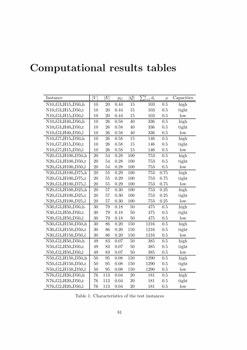
Computational results tables
Instance |V | |E| pG |Q| ∑qi=1 di ρ Capacities
N10 G3 H15 D50 h 10 20 0.44 15 103 0.5 highN10 G3 H15 D50 t 10 20 0.44 15 103 0.5 tightN10 G3 H15 D50 l 10 20 0.44 15 103 0.5 low
N10 G3 H40 D50 h 10 26 0.58 40 336 0.5 highN10 G3 H40 D50 t 10 26 0.58 40 336 0.5 tightN10 G3 H40 D50 l 10 26 0.58 40 336 0.5 low
N10 G7 H15 D50 h 10 26 0.58 15 146 0.5 highN10 G7 H15 D50 t 10 26 0.58 15 146 0.5 tightN10 G7 H15 D50 l 10 26 0.58 15 146 0.5 low
N20 G3 H100 D50 h 20 54 0.28 100 753 0.5 highN20 G3 H100 D50 t 20 54 0.28 100 753 0.5 tightN20 G3 H100 D50 l 20 54 0.28 100 753 0.5 low
N20 G3 H100 D75 h 20 55 0.29 100 753 0.75 highN20 G3 H100 D75 t 20 55 0.29 100 753 0.75 tightN20 G3 H100 D75 l 20 55 0.29 100 753 0.75 low
N20 G3 H100 D25 h 20 57 0.30 100 753 0.25 highN20 G3 H100 D25 t 20 57 0.30 100 753 0.25 tightN20 G3 H100 D25 l 20 57 0.30 100 753 0.25 low
N30 G3 H50 D50 h 30 79 0.18 50 475 0.5 highN30 G3 H50 D50 t 30 79 0.18 50 475 0.5 tightN30 G3 H50 D50 l 30 79 0.18 50 475 0.5 low
N30 G3 H150 D50 h 30 86 0.20 150 1216 0.5 highN30 G3 H150 D50 t 30 86 0.20 150 1216 0.5 tightN30 G3 H150 D50 l 30 86 0.20 150 1216 0.5 low
N50 G2 H50 D50 h 49 83 0.07 50 385 0.5 highN50 G2 H50 D50 t 49 83 0.07 50 385 0.5 tightN50 G2 H50 D50 l 49 83 0.07 50 385 0.5 low
N50 G2 H150 D50 h 50 95 0.08 150 1290 0.5 highN50 G2 H150 D50 t 50 95 0.08 150 1290 0.5 tightN50 G2 H150 D50 l 50 95 0.08 150 1290 0.5 low
N76 G2 H20 D50 h 76 113 0.04 20 181 0.5 highN76 G2 H20 D50 t 76 113 0.04 20 181 0.5 tightN76 G2 H20 D50 l 76 113 0.04 20 181 0.5 low
Table 1: Characteristics of the test instances
81
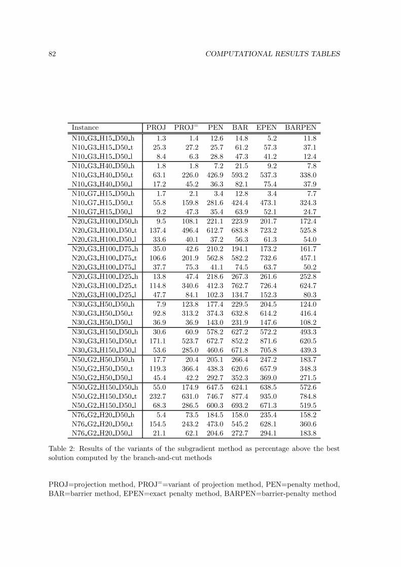
82 COMPUTATIONAL RESULTS TABLES
Instance PROJ PROJ= PEN BAR EPEN BARPEN
N10 G3 H15 D50 h 1.3 1.4 12.6 14.8 5.2 11.8N10 G3 H15 D50 t 25.3 27.2 25.7 61.2 57.3 37.1N10 G3 H15 D50 l 8.4 6.3 28.8 47.3 41.2 12.4
N10 G3 H40 D50 h 1.8 1.8 7.2 21.5 9.2 7.8N10 G3 H40 D50 t 63.1 226.0 426.9 593.2 537.3 338.0N10 G3 H40 D50 l 17.2 45.2 36.3 82.1 75.4 37.9
N10 G7 H15 D50 h 1.7 2.1 3.4 12.8 3.4 7.7N10 G7 H15 D50 t 55.8 159.8 281.6 424.4 473.1 324.3N10 G7 H15 D50 l 9.2 47.3 35.4 63.9 52.1 24.7
N20 G3 H100 D50 h 9.5 108.1 221.1 223.9 201.7 172.4N20 G3 H100 D50 t 137.4 496.4 612.7 683.8 723.2 525.8N20 G3 H100 D50 l 33.6 40.1 37.2 56.3 61.3 54.0
N20 G3 H100 D75 h 35.0 42.6 210.2 194.1 173.2 161.7N20 G3 H100 D75 t 106.6 201.9 562.8 582.2 732.6 457.1N20 G3 H100 D75 l 37.7 75.3 41.1 74.5 63.7 50.2
N20 G3 H100 D25 h 13.8 47.4 218.6 267.3 261.6 252.8N20 G3 H100 D25 t 114.8 340.6 412.3 762.7 726.4 624.7N20 G3 H100 D25 l 47.7 84.1 102.3 134.7 152.3 80.3
N30 G3 H50 D50 h 7.9 123.8 177.4 229.5 204.5 124.0N30 G3 H50 D50 t 92.8 313.2 374.3 632.8 614.2 416.4N30 G3 H50 D50 l 36.9 36.9 143.0 231.9 147.6 108.2
N30 G3 H150 D50 h 30.6 60.9 578.2 627.2 572.2 493.3N30 G3 H150 D50 t 171.1 523.7 672.7 852.2 871.6 620.5N30 G3 H150 D50 l 53.6 285.0 460.6 671.8 705.8 439.3
N50 G2 H50 D50 h 17.7 20.4 205.1 266.4 247.2 183.7N50 G2 H50 D50 t 119.3 366.4 438.3 620.6 657.9 348.3N50 G2 H50 D50 l 45.4 42.2 292.7 352.3 369.0 271.5
N50 G2 H150 D50 h 55.0 174.9 647.5 624.1 638.5 572.6N50 G2 H150 D50 t 232.7 631.0 746.7 877.4 935.0 784.8N50 G2 H150 D50 l 68.3 286.5 600.3 693.2 671.3 519.5
N76 G2 H20 D50 h 5.4 73.5 184.5 158.0 235.4 158.2N76 G2 H20 D50 t 154.5 243.2 473.0 545.2 628.1 360.6N76 G2 H20 D50 l 21.1 62.1 204.6 272.7 294.1 183.8
Table 2: Results of the variants of the subgradient method as percentage above the bestsolution computed by the branch-and-cut methods
PROJ=projection method, PROJ==variant of projection method, PEN=penalty method,BAR=barrier method, EPEN=exact penalty method, BARPEN=barrier-penalty method
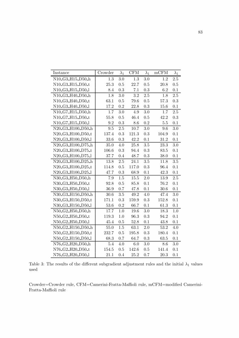
83
Instance Crowder λ1 CFM λ1 mCFM λ1
N10 G3 H15 D50 h 1.3 3.0 1.3 3.0 1.2 2.5N10 G3 H15 D50 t 25.3 0.5 22.7 0.5 20.8 0.5N10 G3 H15 D50 l 8.4 0.3 7.1 0.3 6.2 0.1
N10 G3 H40 D50 h 1.8 3.0 3.2 2.5 1.8 2.5N10 G3 H40 D50 t 63.1 0.5 79.6 0.5 57.3 0.3N10 G3 H40 D50 l 17.2 0.2 22.8 0.3 15.6 0.1
N10 G7 H15 D50 h 1.7 3.0 4.9 3.0 1.7 2.5N10 G7 H15 D50 t 55.8 0.5 46.4 0.5 42.2 0.3N10 G7 H15 D50 l 9.2 0.3 8.6 0.2 5.5 0.1
N20 G3 H100 D50 h 9.5 2.5 10.7 3.0 9.6 3.0N20 G3 H100 D50 t 137.4 0.3 121.3 0.3 104.9 0.1N20 G3 H100 D50 l 33.6 0.3 42.2 0.1 31.2 0.1
N20 G3 H100 D75 h 35.0 4.0 25.8 3.5 23.3 3.0N20 G3 H100 D75 t 106.6 0.3 94.4 0.3 83.5 0.1N20 G3 H100 D75 l 37.7 0.4 48.7 0.3 38.0 0.1
N20 G3 H100 D25 h 13.8 2.5 24.1 3.5 11.8 3.5N20 G3 H100 D25 t 114.8 0.5 117.0 0.3 96.4 0.1N20 G3 H100 D25 l 47.7 0.3 68.9 0.1 42.3 0.1
N30 G3 H50 D50 h 7.9 1.5 15.5 2.0 13.9 2.5N30 G3 H50 D50 t 92.8 0.5 85.8 0.1 76.2 0.1N30 G3 H50 D50 l 36.9 0.7 47.8 0.1 30.6 0.1
N30 G3 H150 D50 h 30.6 3.5 49.2 4.0 47.4 3.0N30 G3 H150 D50 t 171.1 0.3 159.9 0.3 152.8 0.1N30 G3 H150 D50 l 53.6 0.2 66.7 0.1 61.3 0.1
N50 G2 H50 D50 h 17.7 1.0 19.6 3.0 18.3 1.0N50 G2 H50 D50 t 119.3 1.0 96.3 0.3 94.2 0.1N50 G2 H50 D50 l 45.4 0.5 52.8 0.1 43.8 0.1
N50 G2 H150 D50 h 55.0 1.5 63.1 2.0 53.2 4.0N50 G2 H150 D50 t 232.7 0.5 195.8 0.3 180.4 0.1N50 G2 H150 D50 l 68.3 0.7 64.7 0.3 63.5 0.1
N76 G2 H20 D50 h 5.4 4.0 6.0 3.0 8.6 3.0N76 G2 H20 D50 t 154.5 0.5 142.6 0.5 141.4 0.1N76 G2 H20 D50 l 21.1 0.4 25.2 0.7 20.3 0.1
Table 3: The results of the different subgradient adjustment rules and the initial λ1 valuesused
Crowder=Crowder rule, CFM=Camerini-Fratta-Maffioli rule, mCFM=modified Camerini-Fratta-Maffioli rule
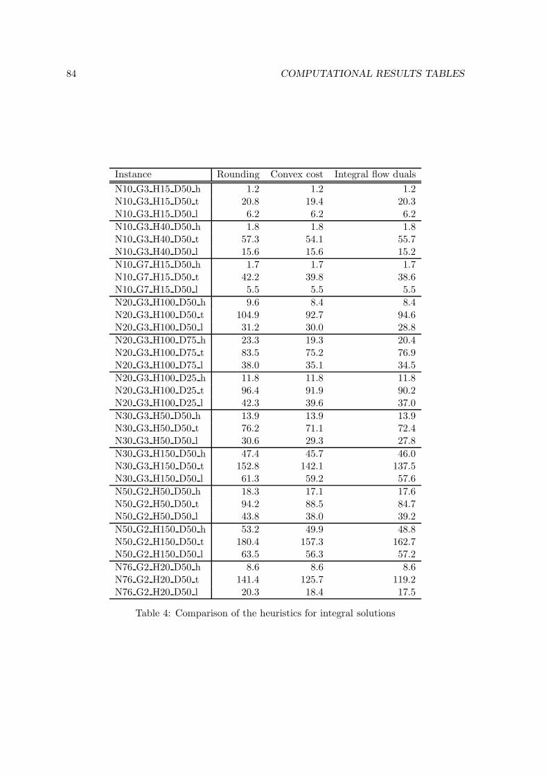
84 COMPUTATIONAL RESULTS TABLES
Instance Rounding Convex cost Integral flow duals
N10 G3 H15 D50 h 1.2 1.2 1.2N10 G3 H15 D50 t 20.8 19.4 20.3N10 G3 H15 D50 l 6.2 6.2 6.2
N10 G3 H40 D50 h 1.8 1.8 1.8N10 G3 H40 D50 t 57.3 54.1 55.7N10 G3 H40 D50 l 15.6 15.6 15.2
N10 G7 H15 D50 h 1.7 1.7 1.7N10 G7 H15 D50 t 42.2 39.8 38.6N10 G7 H15 D50 l 5.5 5.5 5.5
N20 G3 H100 D50 h 9.6 8.4 8.4N20 G3 H100 D50 t 104.9 92.7 94.6N20 G3 H100 D50 l 31.2 30.0 28.8
N20 G3 H100 D75 h 23.3 19.3 20.4N20 G3 H100 D75 t 83.5 75.2 76.9N20 G3 H100 D75 l 38.0 35.1 34.5
N20 G3 H100 D25 h 11.8 11.8 11.8N20 G3 H100 D25 t 96.4 91.9 90.2N20 G3 H100 D25 l 42.3 39.6 37.0
N30 G3 H50 D50 h 13.9 13.9 13.9N30 G3 H50 D50 t 76.2 71.1 72.4N30 G3 H50 D50 l 30.6 29.3 27.8
N30 G3 H150 D50 h 47.4 45.7 46.0N30 G3 H150 D50 t 152.8 142.1 137.5N30 G3 H150 D50 l 61.3 59.2 57.6
N50 G2 H50 D50 h 18.3 17.1 17.6N50 G2 H50 D50 t 94.2 88.5 84.7N50 G2 H50 D50 l 43.8 38.0 39.2
N50 G2 H150 D50 h 53.2 49.9 48.8N50 G2 H150 D50 t 180.4 157.3 162.7N50 G2 H150 D50 l 63.5 56.3 57.2
N76 G2 H20 D50 h 8.6 8.6 8.6N76 G2 H20 D50 t 141.4 125.7 119.2N76 G2 H20 D50 l 20.3 18.4 17.5
Table 4: Comparison of the heuristics for integral solutions
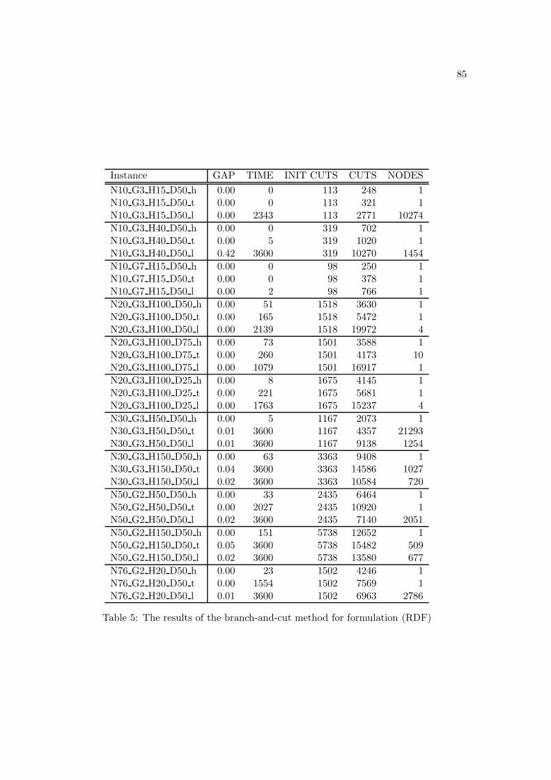
85
Instance GAP TIME INIT CUTS CUTS NODES
N10 G3 H15 D50 h 0.00 0 113 248 1N10 G3 H15 D50 t 0.00 0 113 321 1N10 G3 H15 D50 l 0.00 2343 113 2771 10274
N10 G3 H40 D50 h 0.00 0 319 702 1N10 G3 H40 D50 t 0.00 5 319 1020 1N10 G3 H40 D50 l 0.42 3600 319 10270 1454
N10 G7 H15 D50 h 0.00 0 98 250 1N10 G7 H15 D50 t 0.00 0 98 378 1N10 G7 H15 D50 l 0.00 2 98 766 1
N20 G3 H100 D50 h 0.00 51 1518 3630 1N20 G3 H100 D50 t 0.00 165 1518 5472 1N20 G3 H100 D50 l 0.00 2139 1518 19972 4
N20 G3 H100 D75 h 0.00 73 1501 3588 1N20 G3 H100 D75 t 0.00 260 1501 4173 10N20 G3 H100 D75 l 0.00 1079 1501 16917 1
N20 G3 H100 D25 h 0.00 8 1675 4145 1N20 G3 H100 D25 t 0.00 221 1675 5681 1N20 G3 H100 D25 l 0.00 1763 1675 15237 4
N30 G3 H50 D50 h 0.00 5 1167 2073 1N30 G3 H50 D50 t 0.01 3600 1167 4357 21293N30 G3 H50 D50 l 0.01 3600 1167 9138 1254
N30 G3 H150 D50 h 0.00 63 3363 9408 1N30 G3 H150 D50 t 0.04 3600 3363 14586 1027N30 G3 H150 D50 l 0.02 3600 3363 10584 720
N50 G2 H50 D50 h 0.00 33 2435 6464 1N50 G2 H50 D50 t 0.00 2027 2435 10920 1N50 G2 H50 D50 l 0.02 3600 2435 7140 2051
N50 G2 H150 D50 h 0.00 151 5738 12652 1N50 G2 H150 D50 t 0.05 3600 5738 15482 509N50 G2 H150 D50 l 0.02 3600 5738 13580 677
N76 G2 H20 D50 h 0.00 23 1502 4246 1N76 G2 H20 D50 t 0.00 1554 1502 7569 1N76 G2 H20 D50 l 0.01 3600 1502 6963 2786
Table 5: The results of the branch-and-cut method for formulation (RDF)
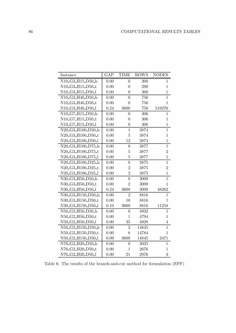
86 COMPUTATIONAL RESULTS TABLES
Instance GAP TIME ROWS NODES
N10 G3 H15 D50 h 0.00 0 300 1N10 G3 H15 D50 t 0.00 0 290 1N10 G3 H15 D50 l 0.00 0 300 1
N10 G3 H40 D50 h 0.00 0 756 1N10 G3 H40 D50 t 0.00 0 756 1N10 G3 H40 D50 l 0.24 3600 756 519276
N10 G7 H15 D50 h 0.00 0 306 1N10 G7 H15 D50 t 0.00 0 306 1N10 G7 H15 D50 l 0.00 0 306 1
N20 G3 H100 D50 h 0.00 1 3874 1N20 G3 H100 D50 t 0.00 5 3874 1N20 G3 H100 D50 l 0.00 12 3874 1
N20 G3 H100 D75 h 0.00 0 3877 1N20 G3 H100 D75 t 0.00 5 3877 2N20 G3 H100 D75 l 0.00 5 3877 1
N20 G3 H100 D25 h 0.00 0 3875 1N20 G3 H100 D25 t 0.00 2 3875 2N20 G3 H100 D25 l 0.00 2 3875 1
N30 G3 H50 D50 h 0.00 0 3009 1N30 G3 H50 D50 t 0.00 2 3009 1N30 G3 H50 D50 l 0.24 3600 3009 48262
N30 G3 H150 D50 h 0.00 2 8816 1N30 G3 H150 D50 t 0.00 10 8816 1N30 G3 H150 D50 l 0.10 3600 8816 11258
N50 G2 H50 D50 h 0.00 0 4932 1N50 G2 H50 D50 t 0.00 1 4794 1N50 G2 H50 D50 l 0.00 35 4928 4
N50 G2 H150 D50 h 0.00 2 14845 1N50 G2 H150 D50 t 0.00 8 14784 1N50 G2 H150 D50 l 0.09 3600 14845 2471
N76 G2 H20 D50 h 0.00 0 3035 1N76 G2 H20 D50 t 0.00 1 2676 1N76 G2 H20 D50 l 0.00 21 2976 3
Table 6: The results of the branch-and-cut method for formulation (EFF)