Embed Size (px)
Citation preview

Instrumentation and Measurements
Dr. Mohammad Kilani
Analog Electrical Devices and Voltage Dividing Circuits
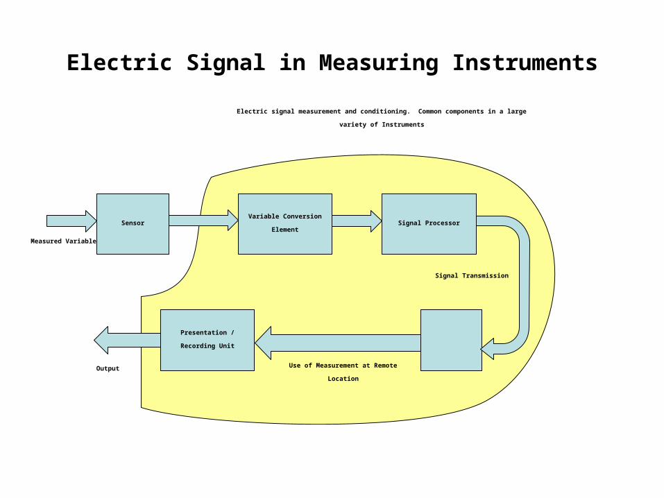
Electric Signal in Measuring Instruments
Measured Variable
Sensor
Electric signal measurement and conditioning. Common components in a large variety of
Instruments
Variable Conversion
ElementSignal Processor
Use of Measurement at Remote
Location
Signal Transmission
Presentation / Recording
Unit
Output
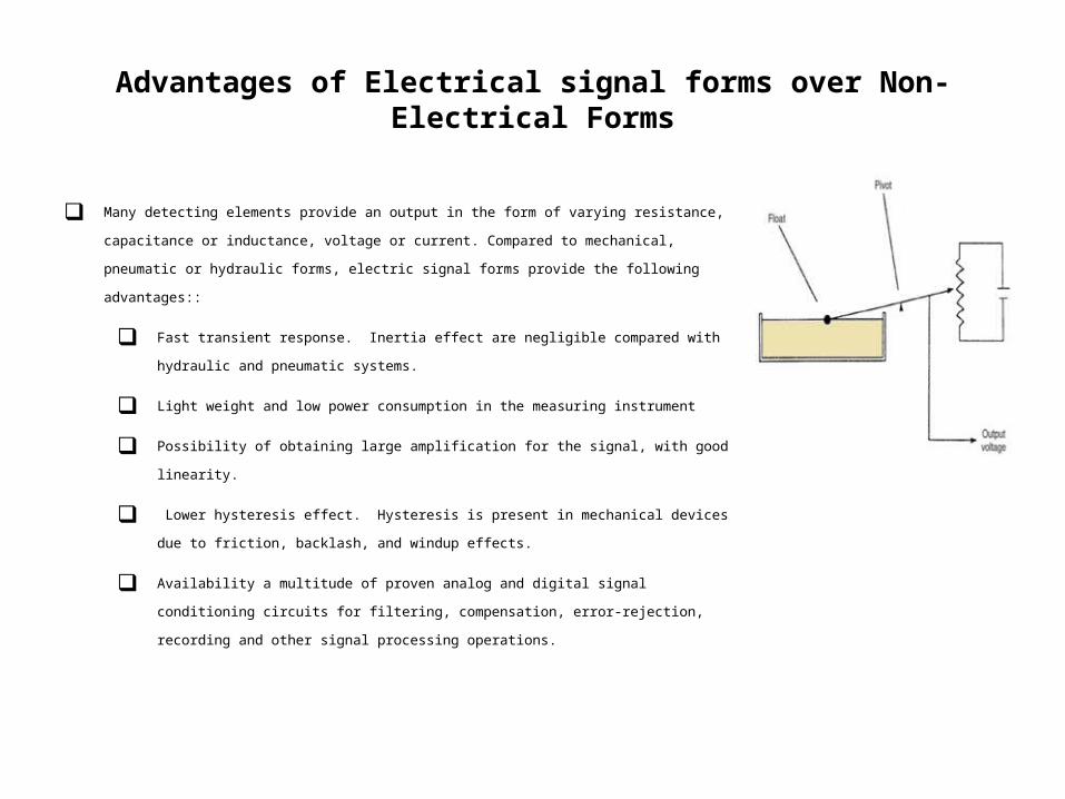
Advantages of Electrical signal forms over Non-Electrical Forms
Many detecting elements provide an output in the form of varying resistance, capacitance or inductance, voltage
or current. Compared to mechanical, pneumatic or hydraulic forms, electric signal forms provide the following
advantages::
Fast transient response. Inertia effect are negligible compared with hydraulic and pneumatic systems.
Light weight and low power consumption in the measuring instrument
Possibility of obtaining large amplification for the signal, with good linearity.
Lower hysteresis effect. Hysteresis is present in mechanical devices due to friction, backlash, and
windup effects.
Availability a multitude of proven analog and digital signal conditioning circuits for filtering,
compensation, error-rejection, recording and other signal processing operations.
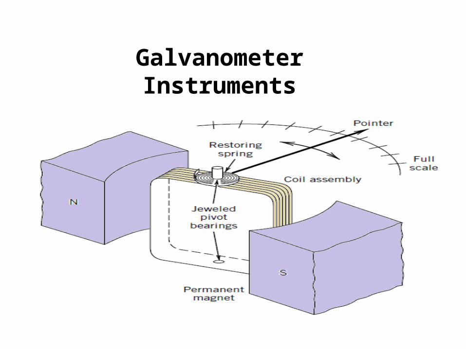
Galvanometer Instruments
Galvanometer Instruments
A galvanometer is an analog device that produces a
deflection proportional to the current in passing in its coil. It
utilizes the principle that a current-carrying conductor
placed in a magnetic field is acted upon by a force that is
proportional to the current passing through the conductor
This force can be used as a measure of the flow of current in
a conductor by moving a pointer on a display.

Galvanometer Instruments:Force on a straight current conductor placed on magnetic field
Consider a straight length l of a conductor through
which a current I flows. The force on this conductor
due to a magnetic field strength B is:
The vector k is a unit vector along the direction of the
current flow, and the force F and the magnetic field B
are also vector quantities.
BIlF
k
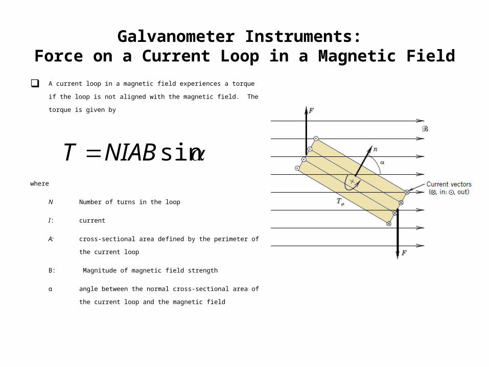
Galvanometer Instruments: Force on a Current Loop in a Magnetic Field
A current loop in a magnetic field experiences a torque if the loop is not aligned
with the magnetic field. The torque is given by
where
N Number of turns in the loop
I: current
A: cross-sectional area defined by the perimeter of the current loop
B: Magnitude of magnetic field strength
α angle between the normal cross-sectional area of the current loop and
the magnetic field
sinNIABT
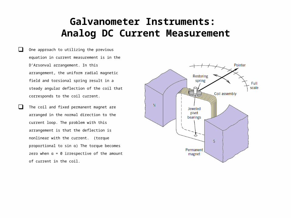
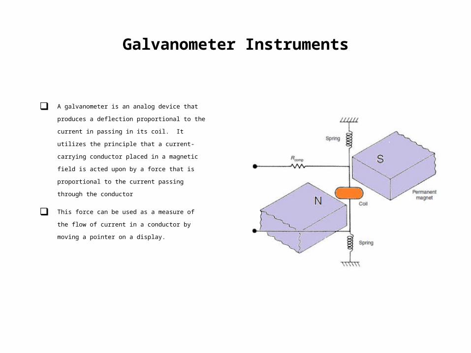
Galvanometer Instruments: Analog DC Current Measurement
One approach to utilizing the previous equation in current
measurement is in the D’Arsonval arrangement. In this
arrangement, the uniform radial magnetic field and torsional
spring result in a steady angular deflection of the coil that
corresponds to the coil current.
The coil and fixed permanent magnet are arranged in the
normal direction to the current loop. The problem with this
arrangement is that the deflection is nonlinear with the
current. (torque proportional to sin α) The torque becomes
zero when α = 0 irrespective of the amount of current in the
coil.
Galvanometer Instruments: Analog DC Current Measurement
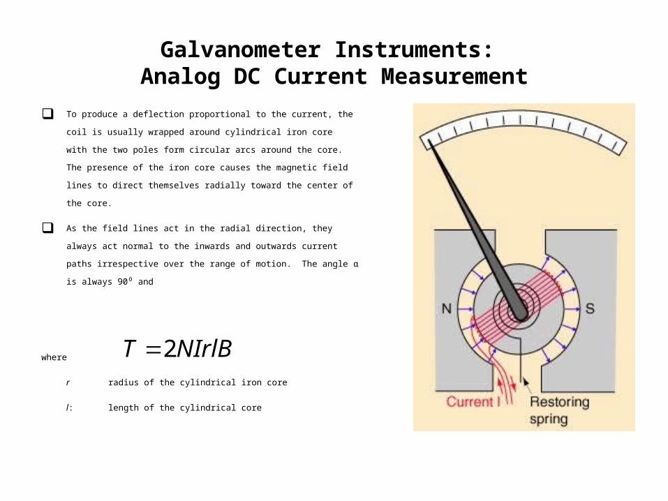
To produce a deflection proportional to the current, the coil is usually wrapped
around cylindrical iron core with the two poles form circular arcs around the core.
The presence of the iron core causes the magnetic field lines to direct themselves
radially toward the center of the core.
As the field lines act in the radial direction, they always act normal to the inwards
and outwards current paths irrespective over the range of motion. The angle α is
always 90⁰ and
where
r radius of the cylindrical iron core
l: length of the cylindrical coreNIrlBT 2
Galvanometer Instruments: Analog DC Current Measurement
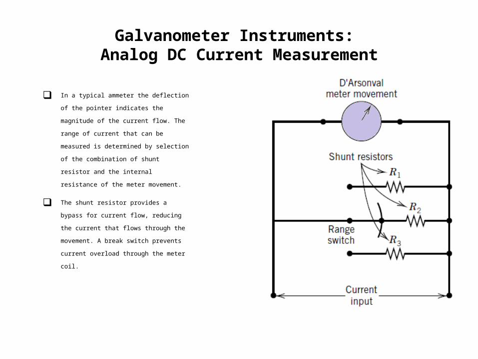
In a typical ammeter the deflection of the pointer
indicates the magnitude of the current flow. The
range of current that can be measured is
determined by selection of the combination of
shunt resistor and the internal resistance of the
meter movement.
The shunt resistor provides a bypass for current
flow, reducing the current that flows through the
movement. A break switch prevents current
overload through the meter coil.
Galvanometer Instruments: Analog DC Current Measurement
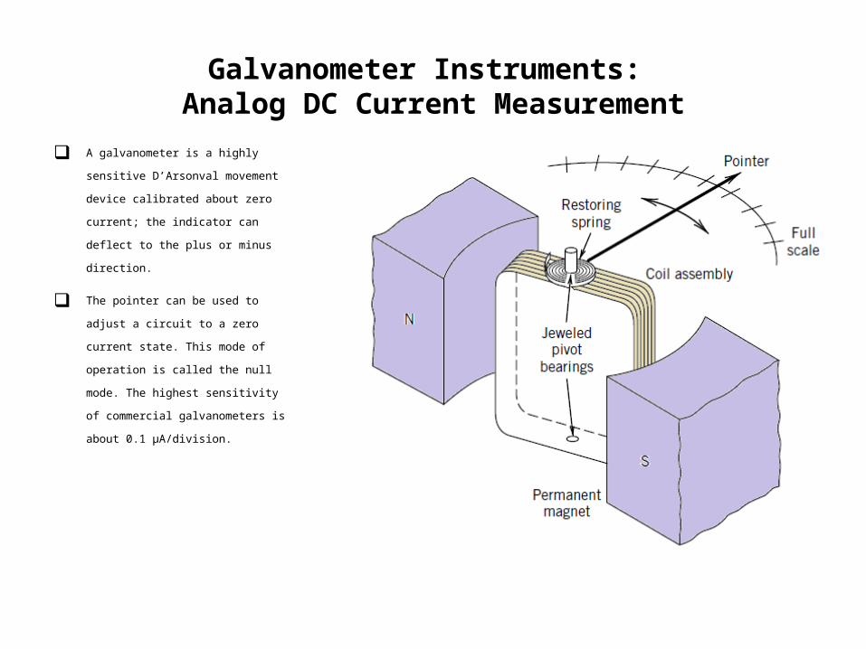
A galvanometer is a highly sensitive
D’Arsonval movement device calibrated
about zero current; the indicator can deflect
to the plus or minus direction.
The pointer can be used to adjust a circuit to
a zero current state. This mode of operation
is called the null mode. The highest
sensitivity of commercial galvanometers is
about 0.1 µA/division.
Galvanometer Instruments: Analog DC Voltage and Resistance Measurement
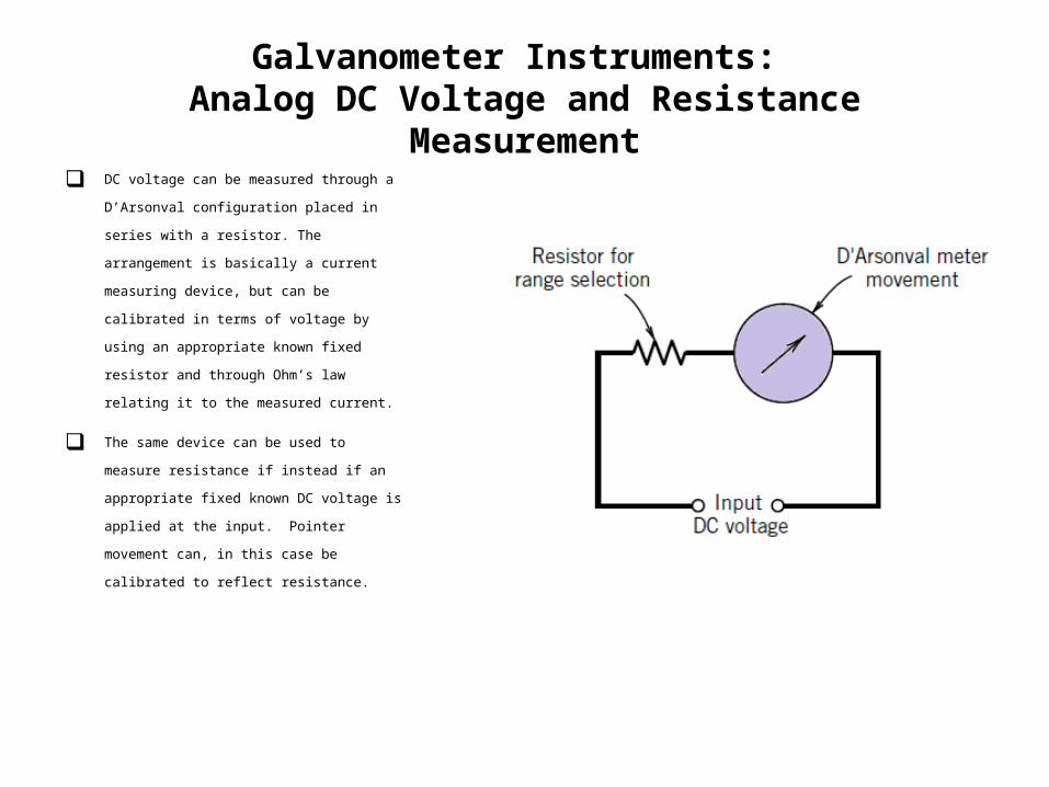
DC voltage can be measured through a D’Arsonval
configuration placed in series with a resistor. The
arrangement is basically a current measuring device,
but can be calibrated in terms of voltage by using an
appropriate known fixed resistor and through Ohm’s
law relating it to the measured current.
The same device can be used to measure resistance if
instead if an appropriate fixed known DC voltage is
applied at the input. Pointer movement can, in this
case be calibrated to reflect resistance.
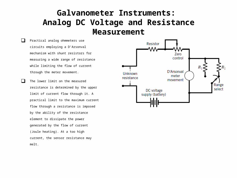
Galvanometer Instruments: Analog DC Voltage and Resistance Measurement
Practical analog ohmmeters use circuits employing a
D’Arsonval mechanism with shunt resistors for measuring
a wide range of resistance while limiting the flow of
current through the meter movement.
The lower limit on the measured resistance is
determined by the upper limit of current flow through it.
A practical limit to the maximum current flow through a
resistance is imposed by the ability of the resistance
element to dissipate the power generated by the flow of
current (Joule heating). At a too high current, the sensor
resistance may melt.

Galvanometer Instruments: Analog DC Voltage and Resistance Measurement
This basic circuit is employed in the construction of analog voltage dials and
volt-ohmmeters (VOMs), which were commonly used for the measurement of
current, voltage, and resistance.
Galvanometer Instruments: Analog AC Current and Voltage Measurement
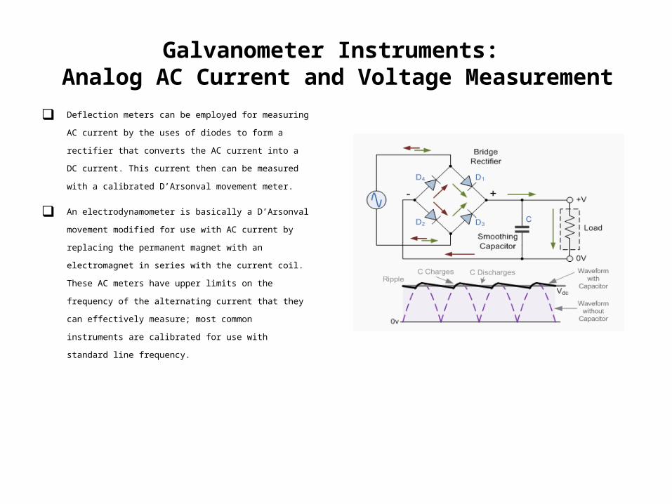
Deflection meters can be employed for measuring AC current by the
uses of diodes to form a rectifier that converts the AC current into a
DC current. This current then can be measured with a calibrated
D’Arsonval movement meter.
An electrodynamometer is basically a D’Arsonval movement modified
for use with AC current by replacing the permanent magnet with an
electromagnet in series with the current coil. These AC meters have
upper limits on the frequency of the alternating current that they can
effectively measure; most common instruments are calibrated for use
with standard line frequency.
Galvanometer Instruments: Analog AC Current and Voltage Measurement
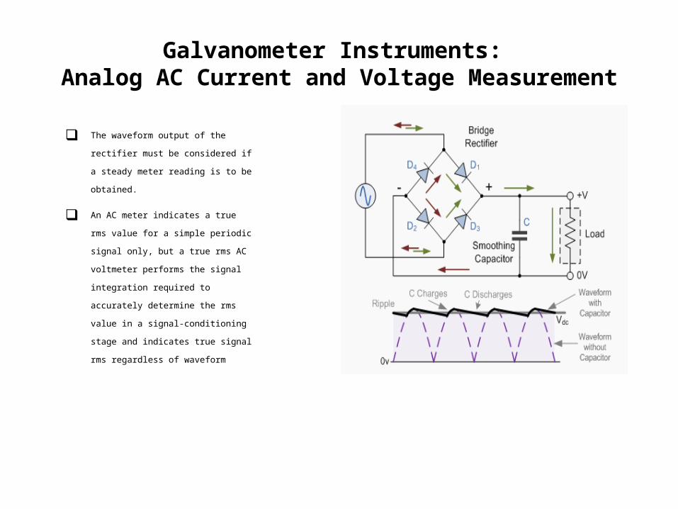
The waveform output of the rectifier must be
considered if a steady meter reading is to be
obtained.
An AC meter indicates a true rms value for a
simple periodic signal only, but a true rms AC
voltmeter performs the signal integration
required to accurately determine the rms
value in a signal-conditioning stage and
indicates true signal rms regardless of
waveform
Galvanometer Instruments: Errors in D’Arsonval Movement
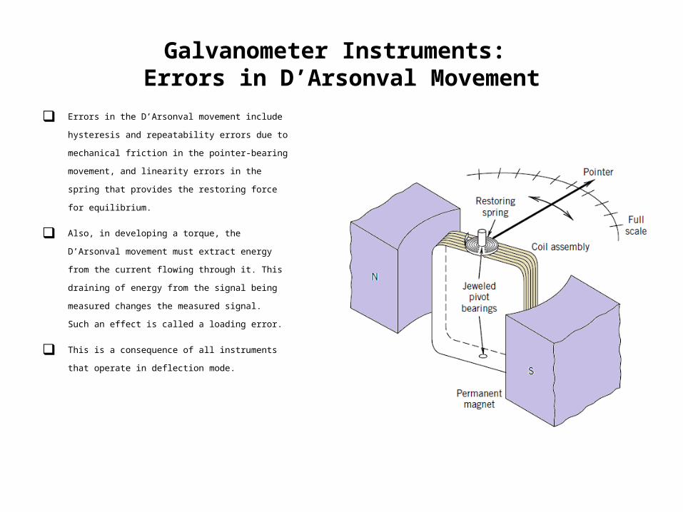
Errors in the D’Arsonval movement include hysteresis and
repeatability errors due to mechanical friction in the pointer-
bearing movement, and linearity errors in the spring that
provides the restoring force for equilibrium.
Also, in developing a torque, the D’Arsonval movement must
extract energy from the current flowing through it. This
draining of energy from the signal being measured changes the
measured signal. Such an effect is called a loading error.
This is a consequence of all instruments that operate in
deflection mode.
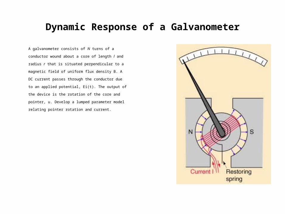
Dynamic Response of a Galvanometer
A galvanometer consists of N turns of a conductor wound about a
core of length l and radius r that is situated perpendicular to a
magnetic field of uniform flux density B. A DC current passes
through the conductor due to an applied potential, Ei(t). The
output of the device is the rotation of the core and pointer, u.
Develop a lumped parameter model relating pointer rotation and
current.
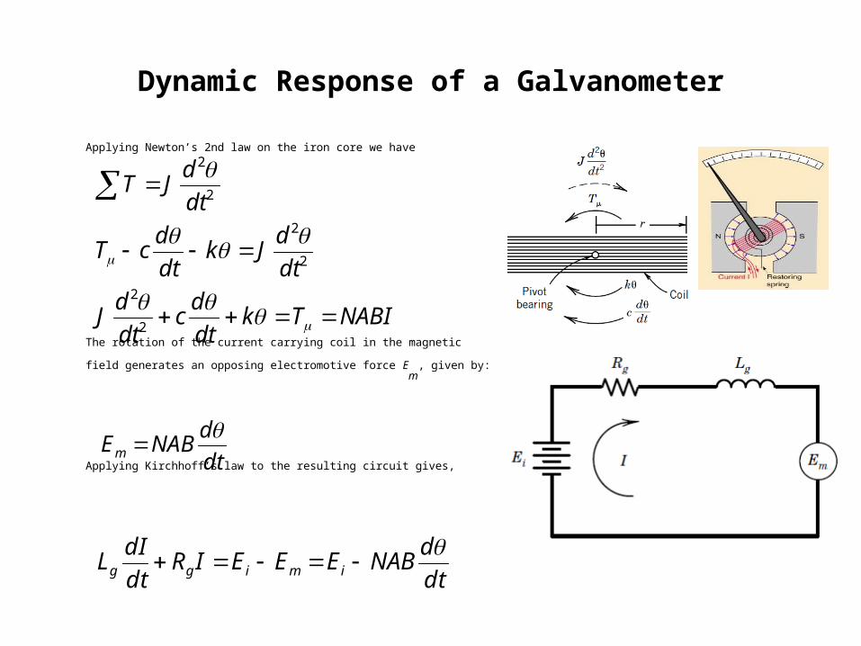
Dynamic Response of a Galvanometer
Applying Newton’s 2nd law on the iron core we have
The rotation of the current carrying coil in the magnetic field generates an opposing
electromotive force Em
, given by:
Applying Kirchhoff’s law to the resulting circuit gives,
NABITkdt
dc
dt
dJ
dt
dJk
dt
dcT
dt
dJT
2
2
2
2
2
2
dt
dNABEm
dt
dNABEEEIR
dt
dIL imigg
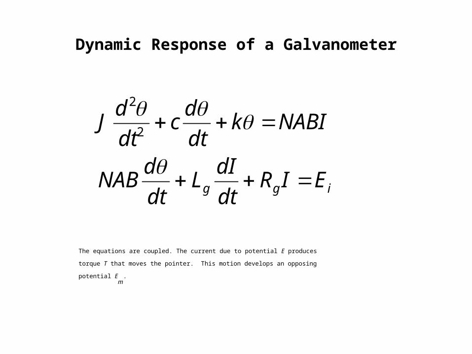
Dynamic Response of a Galvanometer
The equations are coupled. The current due to potential E produces torque T that moves the pointer.
This motion develops an opposing potential Em
.
igg EIRdt
dIL
dt
dNAB
NABIkdt
dc
dt
dJ
2
2
Dynamic Response of a Galvanometer
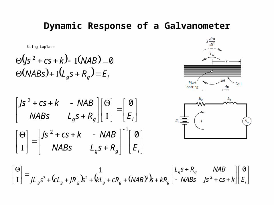
Using Laplace
igg
igg
igg
ERsLNABs
NABkcsJs
ERsLNABs
NABkcsJs
ERsLNABs
NABkcsJs
0
0
0
12
2
2
i
gg
gggggg EkcsJsNABs
NABRsL
kRsNABcRkLsJRcLsJL
012223
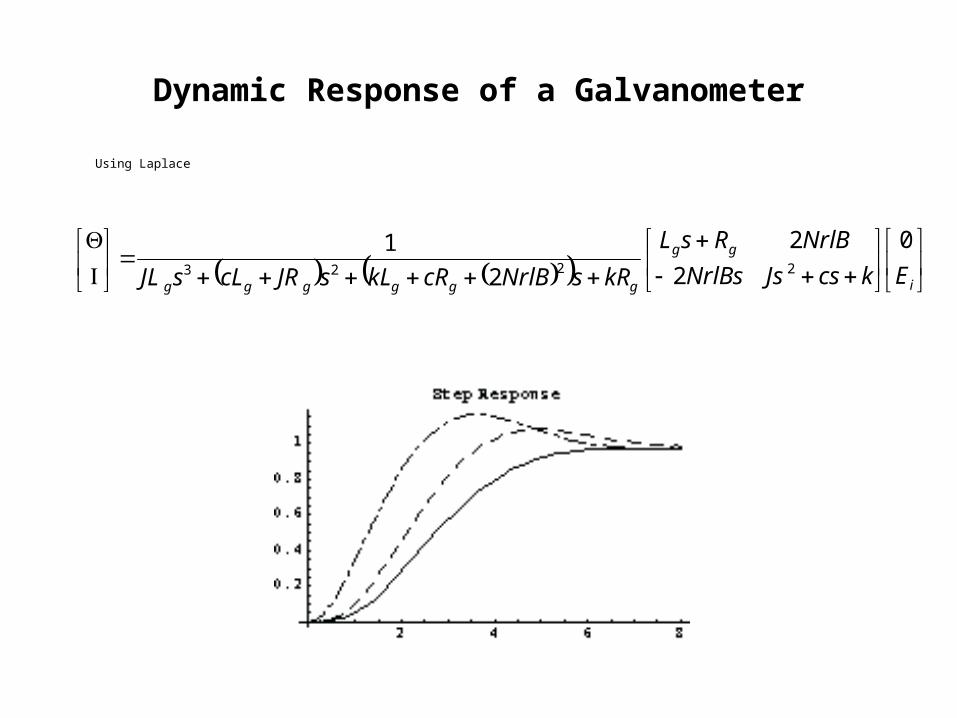
Dynamic Response of a Galvanometer
Using Laplace
i
gg
gggggg EkcsJsNrlBs
NrlBRsL
kRsNrlBcRkLsJRcLsJL
0
2
2
2
12223
Dynamic Response of a Galvanometer
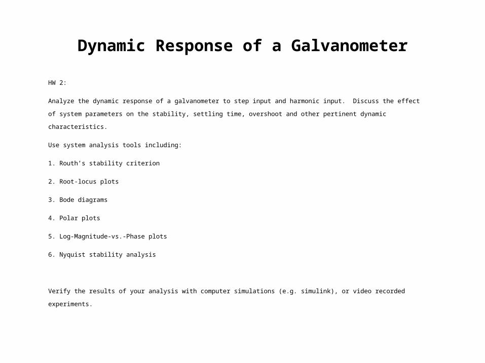
HW 2:
Analyze the dynamic response of a galvanometer to step input and harmonic input. Discuss the effect of system parameters on the stability, settling
time, overshoot and other pertinent dynamic characteristics.
Use system analysis tools including:
1. Routh’s stability criterion
2. Root-locus plots
3. Bode diagrams
4. Polar plots
5. Log-Magnitude-vs.-Phase plots
6. Nyquist stability analysis
Verify the results of your analysis with computer simulations (e.g. simulink), or video recorded experiments.
The Oscilloscope
The Oscilloscope
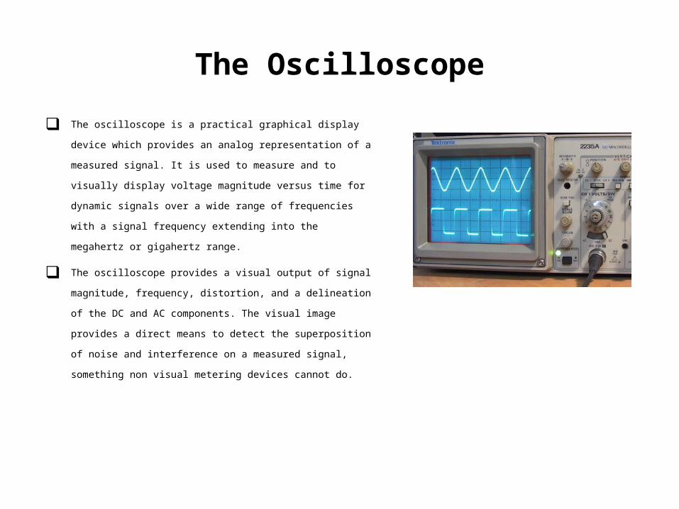
The oscilloscope is a practical graphical display device which provides an
analog representation of a measured signal. It is used to measure and to
visually display voltage magnitude versus time for dynamic signals over a
wide range of frequencies with a signal frequency extending into the
megahertz or gigahertz range.
The oscilloscope provides a visual output of signal magnitude, frequency,
distortion, and a delineation of the DC and AC components. The visual
image provides a direct means to detect the superposition of noise and
interference on a measured signal, something non visual metering devices
cannot do.
The Oscilloscope
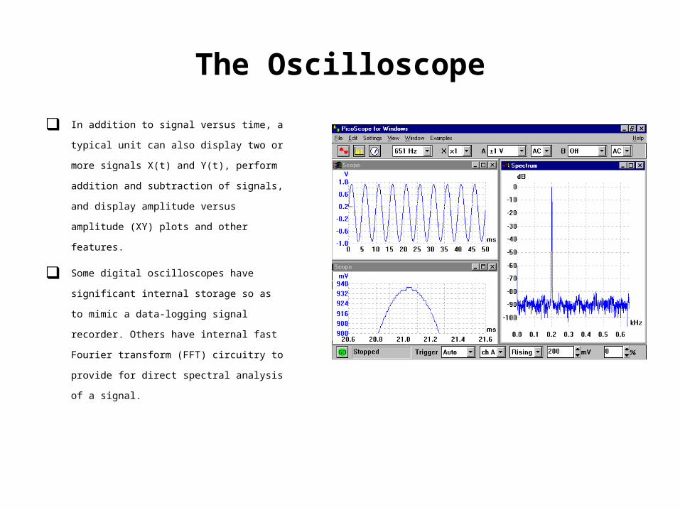
In addition to signal versus time, a typical unit can
also display two or more signals X(t) and Y(t), perform
addition and subtraction of signals, and display
amplitude versus amplitude (XY) plots and other
features.
Some digital oscilloscopes have significant internal
storage so as to mimic a data-logging signal recorder.
Others have internal fast Fourier transform (FFT)
circuitry to provide for direct spectral analysis of a
signal.
The Oscilloscope
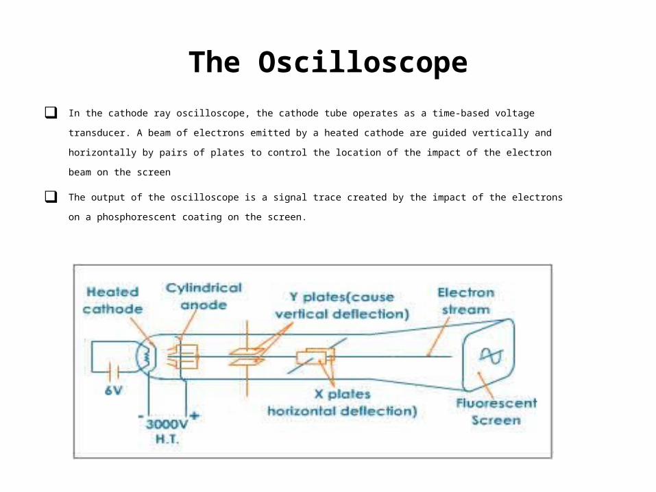
In the cathode ray oscilloscope, the cathode tube operates as a time-based voltage transducer. A beam of electrons emitted by a
heated cathode are guided vertically and horizontally by pairs of plates to control the location of the impact of the electron beam
on the screen
The output of the oscilloscope is a signal trace created by the impact of the electrons on a phosphorescent coating on the screen.
The Oscilloscope
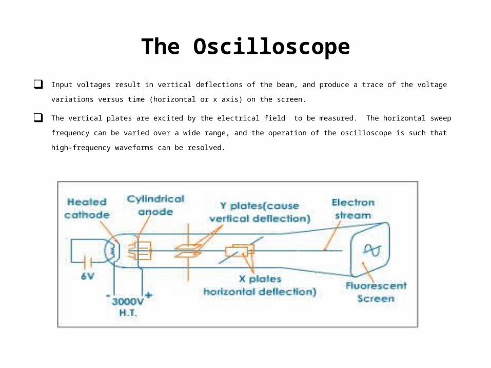
Input voltages result in vertical deflections of the beam, and produce a trace of the voltage variations versus time (horizontal or x axis) on
the screen.
The vertical plates are excited by the electrical field to be measured. The horizontal sweep frequency can be varied over a wide range,
and the operation of the oscilloscope is such that high-frequency waveforms can be resolved.
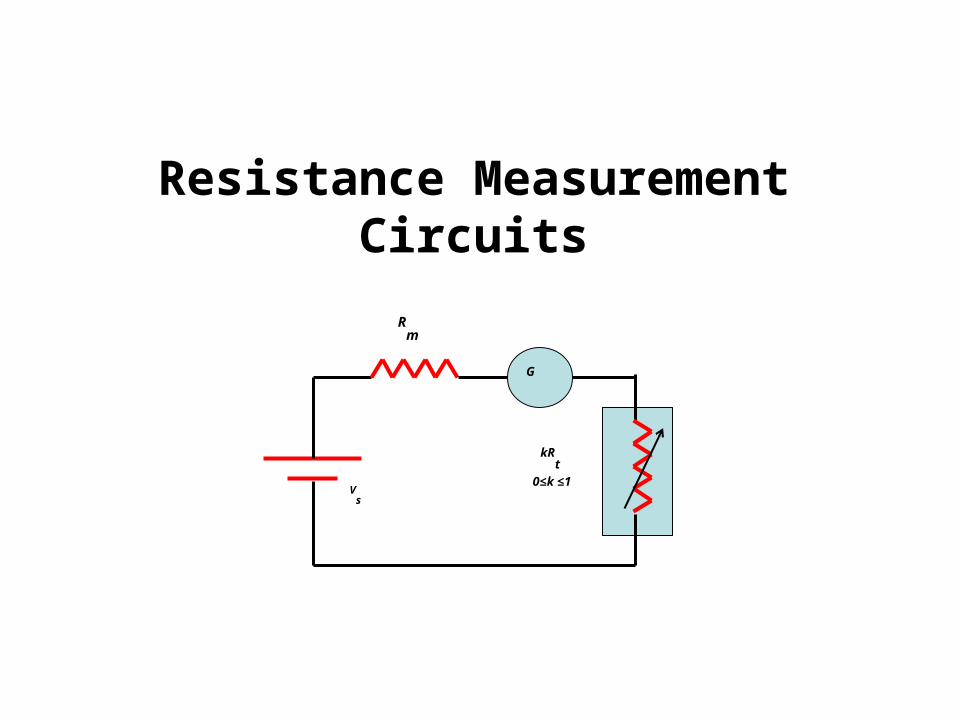
Resistance Measurement Circuits
Vs
Rm
G
kRt
0≤k ≤1
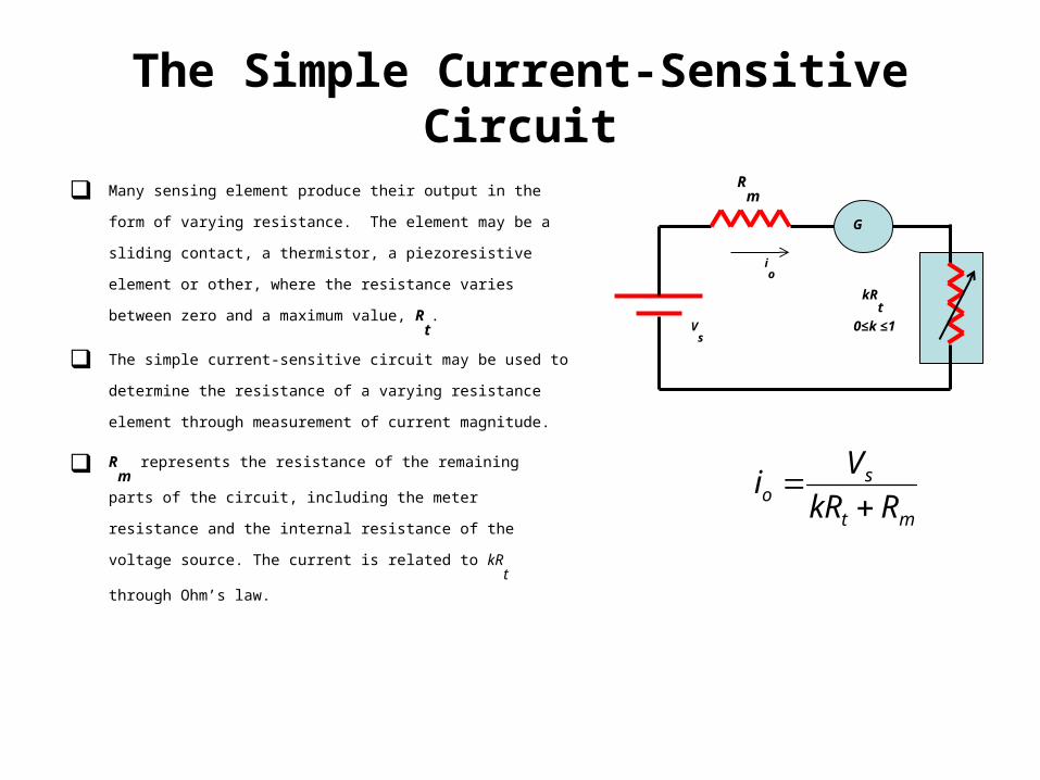
The Simple Current-Sensitive Circuit
Many sensing element produce their output in the form of varying
resistance. The element may be a sliding contact, a thermistor, a
piezoresistive element or other, where the resistance varies between zero
and a maximum value, Rt.
The simple current-sensitive circuit may be used to determine the
resistance of a varying resistance element through measurement of
current magnitude.
Rm
represents the resistance of the remaining parts of the circuit,
including the meter resistance and the internal resistance of the voltage
source. The current is related to kRt through Ohm’s law.
mt
so RkR
Vi
Vs
Rm
G
kRt
0≤k ≤1
io
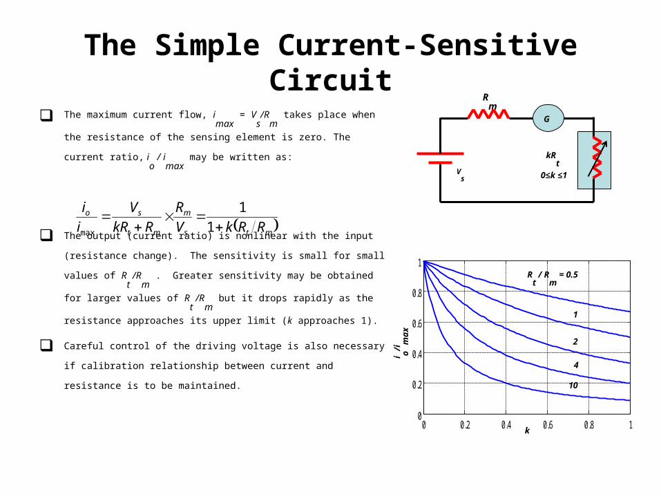
The Simple Current-Sensitive Circuit
The maximum current flow, imax
= Vs/R
m takes place when the resistance of the
sensing element is zero. The current ratio, io
/ imax
may be written as:
The output (current ratio) is nonlinear with the input (resistance change). The
sensitivity is small for small values of Rt
/Rm
. Greater sensitivity may be obtained
for larger values of Rt
/Rm
but it drops rapidly as the resistance approaches its upper
limit (k approaches 1).
Careful control of the driving voltage is also necessary if calibration relationship
between current and resistance is to be maintained.
mts
m
mt
so
RRkV
R
RkR
V
i
i
1
1
max
Vs
Rm
G
kRt
0≤k ≤1
0 0.2 0.4 0.6 0.8 10
0.2
0.4
0.6
0.8
1R
t / R
m = 0.5
1
2
4
10
k
i o/im
ax
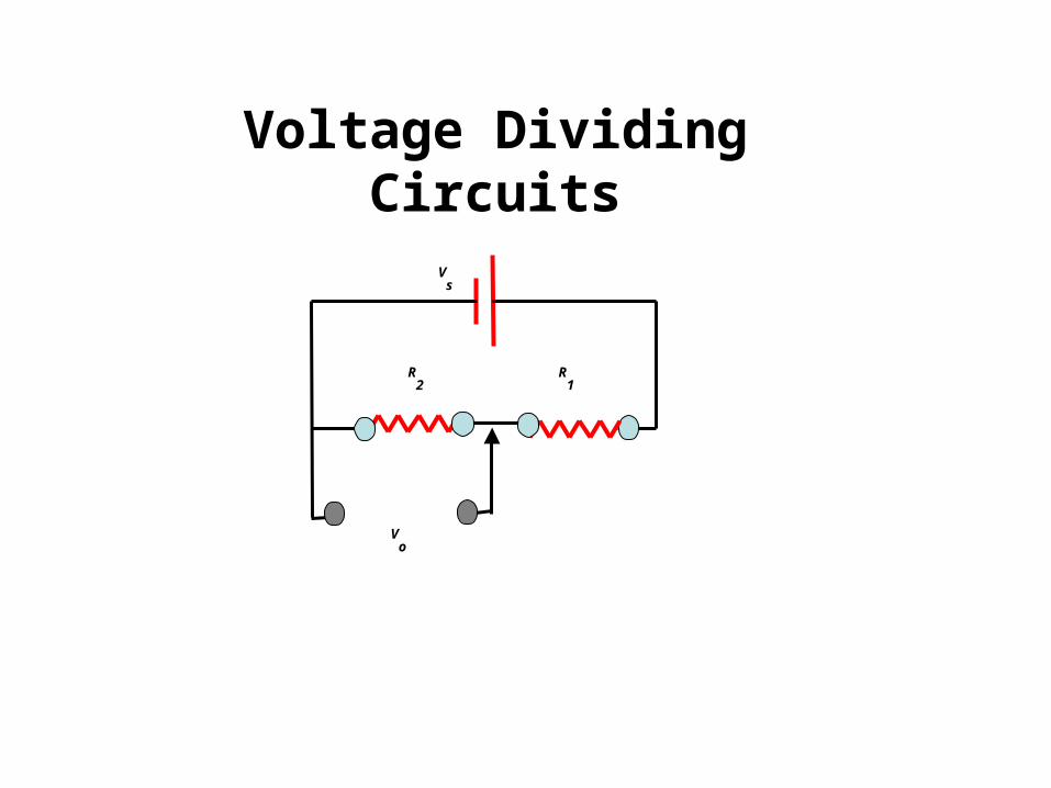
Voltage Dividing Circuits
Vs
R1
R2
Vo
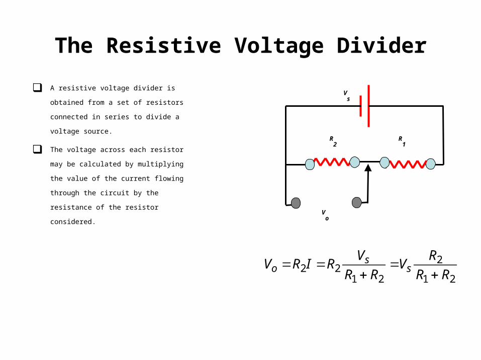
The Resistive Voltage Divider
A resistive voltage divider is obtained from a set
of resistors connected in series to divide a
voltage source.
The voltage across each resistor may be
calculated by multiplying the value of the current
flowing through the circuit by the resistance of
the resistor considered.
21
2
2122 RR
RV
RR
VRIRV s
so
Vs
R1
R2
Vo
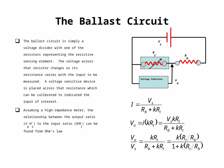
The Ballast Circuit
The ballast circuit is simply a voltage divider with one of
the resistors representing the resistive sensing element.
The voltage across that resistor changes as its resistance
varies with the input to be measured. A voltage sensitive
device is placed across that resistance which can be
calibrated to indicated the input of interest.
Assuming a high-impedance meter, the relationship
between the output ratio (Vo
/Vs) to the input ratio
(R/Rt) can be found from Ohm’s law
Vs
Rb
Rt
Vo
Voltage Indicator
bt
bt
tb
t
s
o
tb
tsto
tb
s
RRk
RRk
kRR
kR
V
V
kRR
kRVkRiV
kRR
VI
1
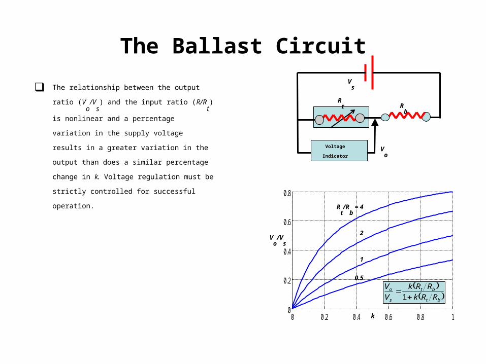
The Ballast Circuit
The relationship between the output ratio (Vo
/Vs) and
the input ratio (R/Rt) is nonlinear and a percentage
variation in the supply voltage results in a greater
variation in the output than does a similar percentage
change in k. Voltage regulation must be strictly
controlled for successful operation.
Vs
Rb
Rt
Vo
Voltage Indicator
0 0.2 0.4 0.6 0.8 10
0.2
0.4
0.6
0.8
k
Vo
/Vs
Rt/R
b = 4
2
1
0.5 bt
bt
s
o
RRk
RRk
V
V
1
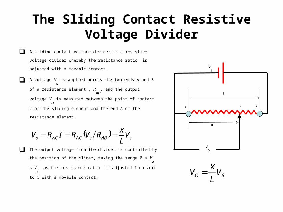
The Sliding Contact Resistive Voltage Divider
A sliding contact voltage divider is a resistive voltage divider whereby the
resistance ratio is adjusted with a movable contact.
A voltage Vs is applied across the two ends A and B of a resistance element ,
RAB
, and the output voltage Vo
is measured between the point of contact C
of the sliding element and the end A of the resistance element.
The output voltage from the divider is controlled by the position of the slider,
taking the range 0 ≤ Vo
≤ Vs. as the resistance ratio is adjusted from zero to
1 with a movable contact. sABsACACo V
L
xRVRIRV
A
Vs
x
L
C B
Vo
so VL
xV
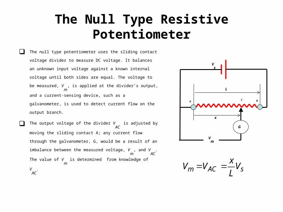
The Null Type Resistive Potentiometer
The null type potentiometer uses the sliding contact voltage divider to
measure DC voltage. It balances an unknown input voltage against a known
internal voltage until both sides are equal. The voltage to be measured, Vm
,
is applied at the divider’s output, and a current-sensing device, such as a
galvanometer, is used to detect current flow on the output branch.
The output voltage of the divider VAC
is adjusted by moving the sliding
contact A; any current flow through the galvanometer, G, would be a result of
an imbalance between the measured voltage, Vm
, and VAC
. The value of Vm
is determined from knowledge of VAC
.
A
Vs
x
L
C B
Vm
G
sACm VL
xVV
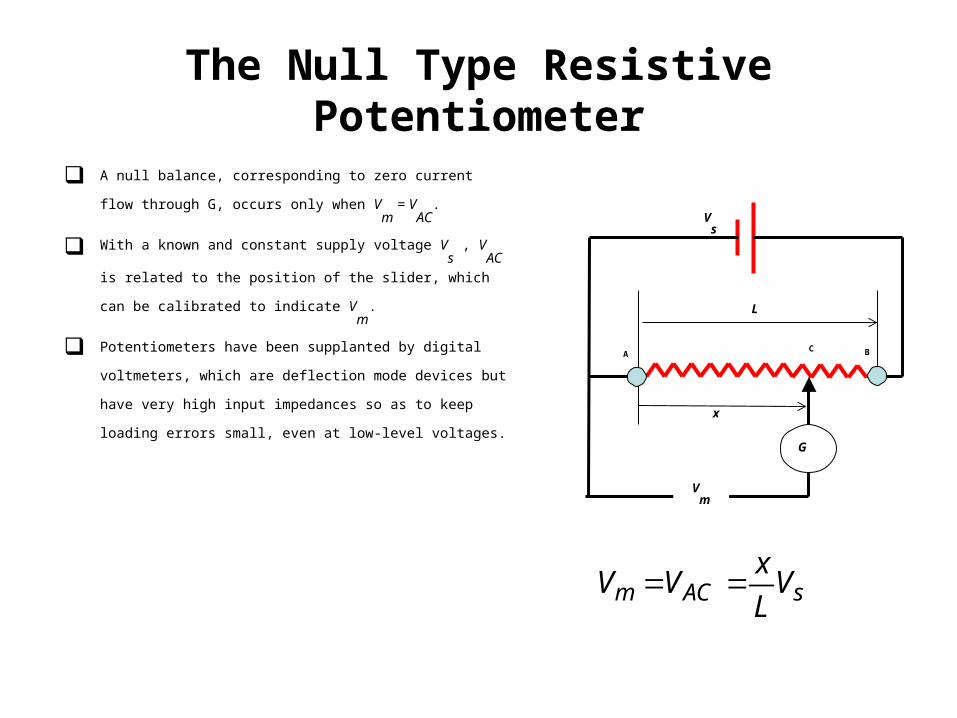
The Null Type Resistive Potentiometer
A null balance, corresponding to zero current flow through G, occurs
only when Vm
= VAC
.
With a known and constant supply voltage Vs , V
AC is related to the
position of the slider, which can be calibrated to indicate Vm
.
Potentiometers have been supplanted by digital voltmeters, which are
deflection mode devices but have very high input impedances so as to
keep loading errors small, even at low-level voltages.
A
Vs
x
L
C B
Vm
G
sACm VL
xVV
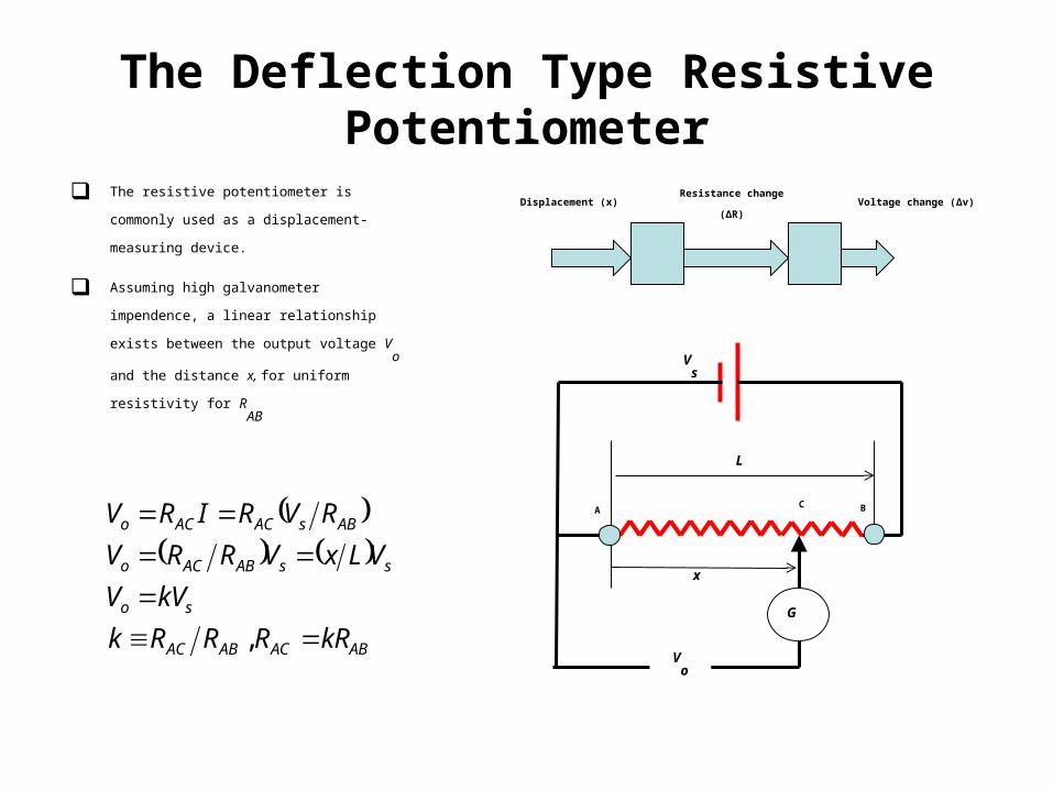
The Deflection Type Resistive Potentiometer
The resistive potentiometer is commonly used as a
displacement-measuring device.
Assuming high galvanometer impendence, a linear
relationship exists between the output voltage Vo
and
the distance x, for uniform resistivity for RAB
Displacement (x)Resistance change (ΔR)
Voltage change (Δv)
A
Vs
x
L
C B
Vo
G
ABACABAC
so
ssABACo
ABsACACo
kRRRRk
kVV
VLxVRRV
RVRIRV
,
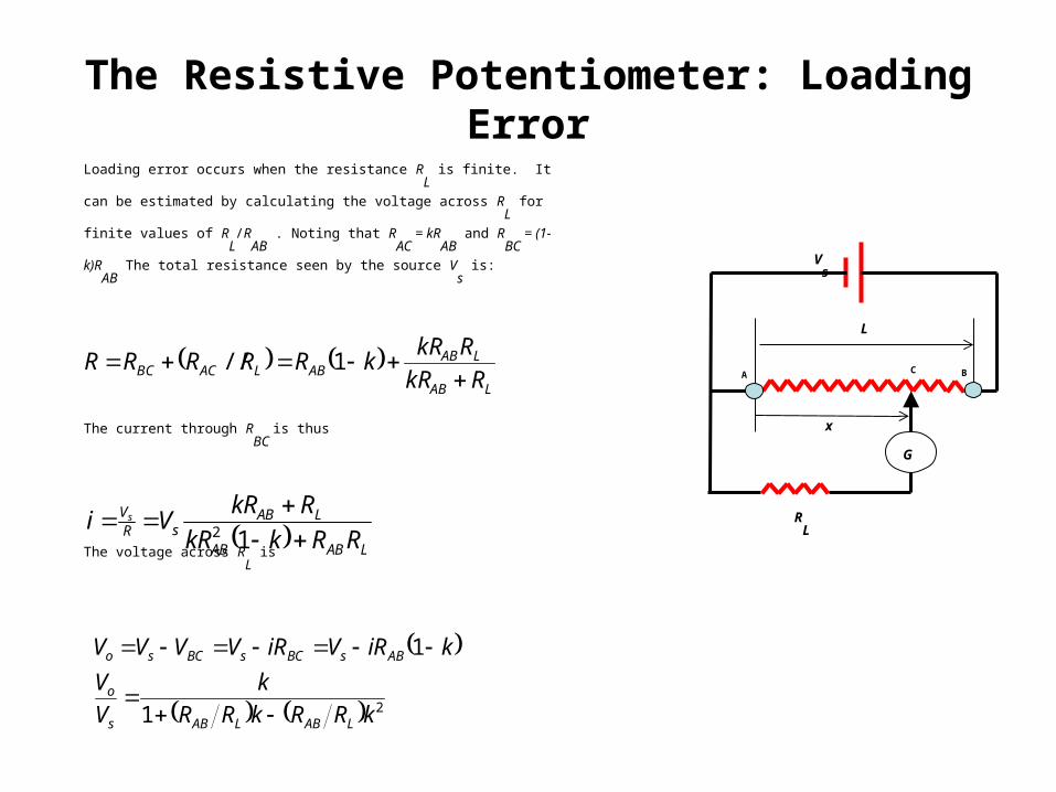
The Resistive Potentiometer: Loading ErrorLoading error occurs when the resistance R
L is finite. It can be estimated by calculating
the voltage across RL for finite values of R
L/R
AB . Noting that R
AC = kR
AB and R
BC = (1-
k)RAB
The total resistance seen by the source Vs is:
The current through RBC
is thus
The voltage across RL is
A
Vs
x
L
C B
RL
G
LAB
LABABLACBC RkR
RkRkRRRRR
1//
LABAB
LABsR
V
RRkkR
RkRVi s
12
21
1
kRRkRR
k
V
V
kiRViRVVVV
LABLABs
o
ABsBCsBCso
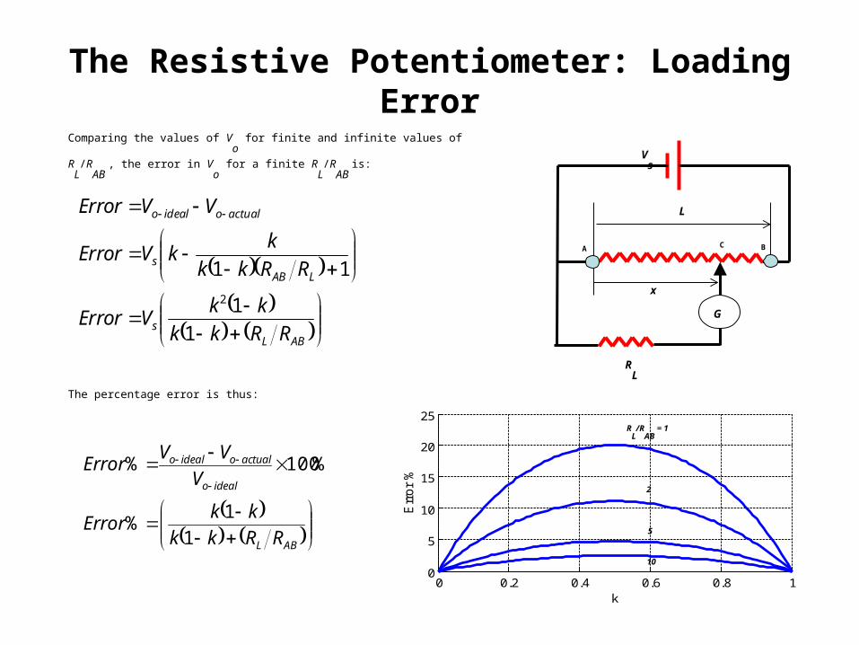
The Resistive Potentiometer: Loading ErrorComparing the values of V
o for finite and infinite values of R
L/R
AB , the error in V
o for a finite
RL/R
AB is:
The percentage error is thus:
A
Vs
x
L
C B
RL
G
ABLs
LABs
actualoidealo
RRkk
kkVError
RRkk
kkVError
VVError
1
1
112
ABL
idealo
actualoidealo
RRkk
kkError
V
VVError
1
1%
%100%
0 0.2 0.4 0.6 0.8 10
5
10
15
20
25
k
Err
or
%
RL
/RAB
= 1
2
5
10
0 0.2 0.4 0.6 0.8 10
5
10
15
k
Err
or
%
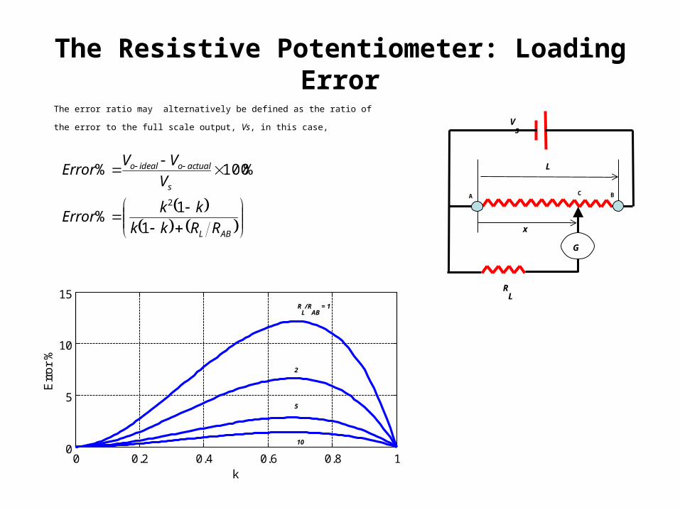
The Resistive Potentiometer: Loading ErrorThe error ratio may alternatively be defined as the ratio of the error to the full scale output,
Vs, in this case,
A
Vs
x
L
C B
RL
G
ABL
s
actualoidealo
RRkk
kkError
V
VVError
1
1%
%100%
2
RL
/RAB
= 1
2
5
10
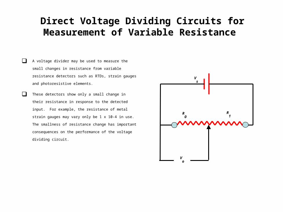
Direct Voltage Dividing Circuits for Measurement of Variable Resistance
A voltage divider may be used to measure the small changes in
resistance from variable resistance detectors such as RTDs, strain
gauges and photoresistive elements.
These detectors show only a small change in their resistance in
response to the detected input. For example, the resistance of metal
strain gauges may vary only be 1 x 10⁻⁴ in use. The smallness of
resistance change has important consequences on the performance of
the voltage dividing circuit.
Vs
R1
Vo
R0
Direct Voltage Dividing Circuits for Measurement of Variable Resistance : Sensitivity
Suppose that a voltage divider is formed from a detector of an initial
resistance R0
and a second resistance with R = R0
. The initial output is:
Assuming no change in the supply voltage during measurement, dVs = 0,
0210
1
10
0
0210
0
1010
0
10
0
1
dRRR
RVdV
RR
RdV
dRRR
R
RRVdV
RR
RdV
VRR
RV
sso
sso
so
Vo
→ Vo
+ Δ Vo
Vs
R1
R0
→ R0
+ ΔR
0201
01
0
0201
201
0210
1
1
1
dRRR
RR
R
VdV
dRRR
RRVdV
dRRR
RVdV
so
so
so
oso
so
sR
Vs
dR
dV
RR
RR
R
V
dR
dV
00
201
01
00 1
Direct Voltage Dividing Circuits for Measurement of Variable Resistance : Sensitivity
The sensitivity of the potentiometer increases with Vs , s
o = r/(1+r2) and with
1/Ro
. Practical considerations place an upper limit on Vs . R
o can not be made
too small as δRo
is related to the value of Ro
. The ratio r = R1
/ Ro
, can be
chosen to maximize so
= r/(1+r2)
Vo
→ Vo
+ Δ Vo
Vs
R1
R0
→ R0
+ ΔR
1,12
1
2
1
1
01
2
1
1
1
33
32
2
rrr
r
r
r
r
r
r
rdr
ds
r
rs
o
o
0 1 2 3 4 5 6 7 8 9 100
0.05
0.1
0.15
0.2
0.25
0.3
01 RRr
21 r
rso
oss
so
sR
V
r
r
R
Vs
RR
RR
R
V
dR
dVs
02
0
201
01
00
1
1
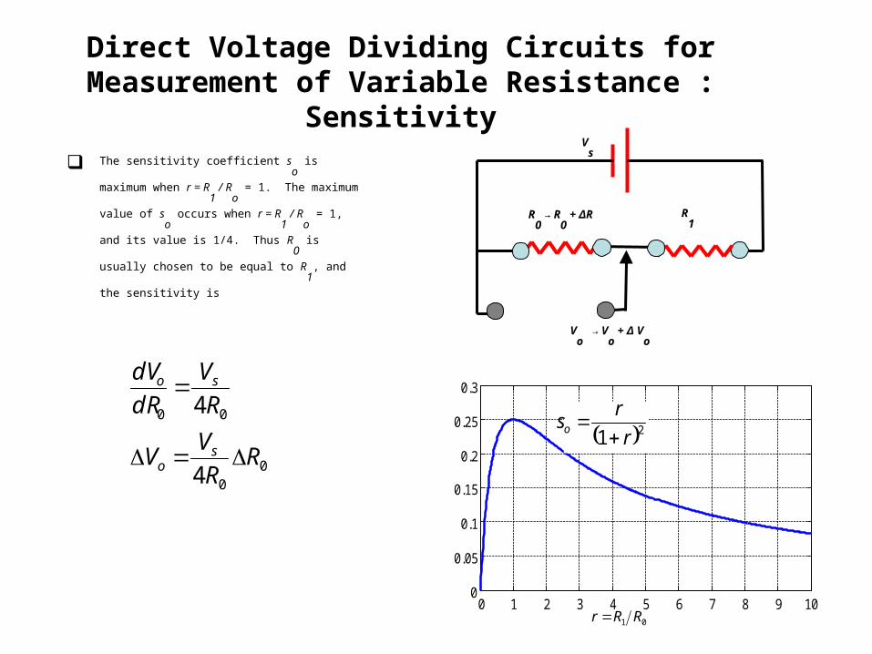
Direct Voltage Dividing Circuits for Measurement of Variable Resistance : Sensitivity
The sensitivity coefficient so
is maximum when r = R1
/ Ro
= 1. The maximum value of so
occurs when r = R1
/ Ro
= 1,
and its value is 1/4. Thus R0
is usually chosen to be equal
to R1
, and the sensitivity is
Vo
→ Vo
+ Δ Vo
Vs
R1
R0
→ R0
+ ΔR
0 1 2 3 4 5 6 7 8 9 100
0.05
0.1
0.15
0.2
0.25
0.3
01 RRr
21 r
rso
00
00
4
4
RR
VV
R
V
dR
dV
so
so
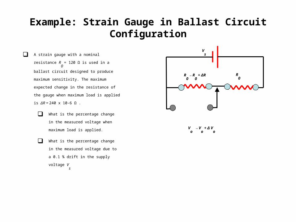
Example: Strain Gauge in Ballast Circuit Configuration
A strain gauge with a nominal resistance R0
= 120 Ω is
used in a ballast circuit designed to produce maximum
sensitivity. The maximum expected change in the
resistance of the gauge when maximum load is applied
is ΔR = 240 x 10-6 Ω .
What is the percentage change in the
measured voltage when maximum load is
applied.
What is the percentage change in the
measured voltage due to a 0.1 % drift in the
supply voltage Vs
Vo
→ Vo
+ Δ Vo
Vs
R0
R0
→ R0
+ ΔR
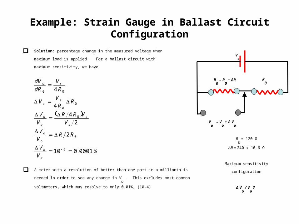
Example: Strain Gauge in Ballast Circuit Configuration
Solution: percentage change in the measured voltage when maximum load is
applied. For a ballast circuit with maximum sensitivity, we have
Vo
→ Vo
+ Δ Vo
Vs
R0
R0
→ R0
+ ΔR
%0001.010
2
2
4
4
4
6
0
0
00
00
o
o
o
o
s
s
o
o
so
so
V
V
RRV
V
V
VRR
V
V
RR
VV
R
V
dR
dV
A meter with a resolution of better than one part in a millionth is needed in order to see any change in
Vo
. This excludes most common voltmeters, which may resolve to only 0.01%, (10-4)
R0
= 120 Ω
ΔR = 240 x 10-6 Ω
Maximum sensitivity configuration
Δ Vo
/ Vo
?
Example: Strain Gauge in Ballast Circuit Configuration
Solution: percentage change in the measured voltage due to a 0.1 %
drift in the supply voltage Vs
The percentage change in the measured voltage due to a 0.1 % the
drift in Vs is 0.1 % which is a 1000 times greater than the strain
induced change in voltage, 0.0001%
Vo
→ Vo
+ Δ Vo
Vs
R0
R0
→ R0
+ ΔR
R0
= 120 Ω
ΔR = 240 x 10-6 Ω
Maximum sensitivity configuration
Δ Vo
/ Vo
?
s
s
o
o
ssso
V
dV
V
dV
dVdVR
RdV
RR
RdV
2
1
2 10
0
10
0
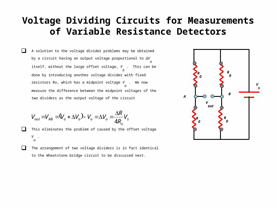
Voltage Dividing Circuits for Measurements of Variable Resistance Detectors
A solution to the voltage divider problems may be obtained by a circuit having an output
voltage proportional to ΔVo
itself, without the large offset voltage, Vo
. This can be done
by introducing another voltage divider with fixed resistors Ro, which has a midpoint
voltage Vo
. We now measure the difference between the midpoint voltages of the two
dividers as the output voltage of the circuit
This eliminates the problem of caused by the offset voltage Vo
.
The arrangement of two voltage dividers is in fact identical to the Wheatstone bridge
circuit to be discussed next.
A
so
ooooABout VR
RVVVVVV
4
B
Vs
R0
R0
R0
R0
Vout
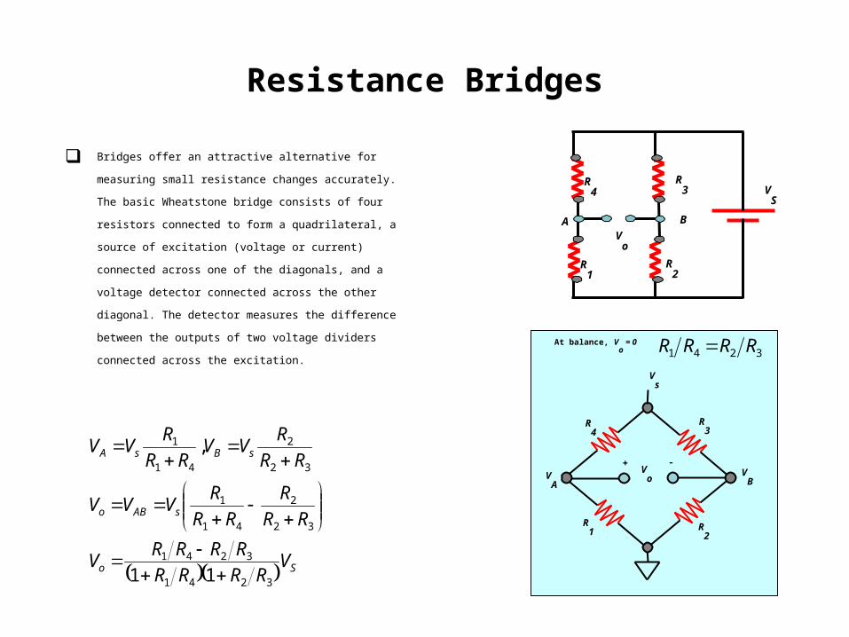
Resistance Bridges
Bridges offer an attractive alternative for measuring small resistance
changes accurately. The basic Wheatstone bridge consists of four
resistors connected to form a quadrilateral, a source of excitation
(voltage or current) connected across one of the diagonals, and a
voltage detector connected across the other diagonal. The detector
measures the difference between the outputs of two voltage dividers
connected across the excitation.
So
sABo
sBsA
VRRRR
RRRRV
RR
R
RR
RVVV
RR
RVV
RR
RVV
3241
3241
32
2
41
1
32
2
41
1
11
,
At balance, Vo
= 0
Vs
R3
R4
R1 R
2
Vo
+ -
3241 RRRR
VB
VA
B
VS
R2
R3
R4
R1
AV
o
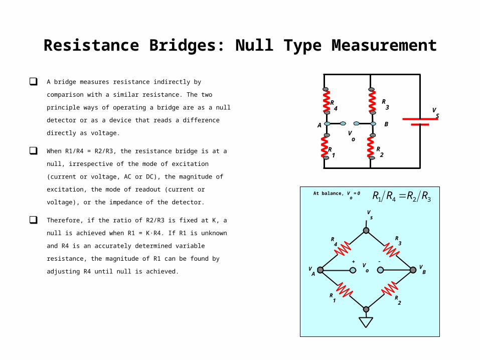
Resistance Bridges: Null Type Measurement
A bridge measures resistance indirectly by comparison with a similar
resistance. The two principle ways of operating a bridge are as a null
detector or as a device that reads a difference directly as voltage.
When R1/R4 = R2/R3, the resistance bridge is at a null, irrespective of the
mode of excitation (current or voltage, AC or DC), the magnitude of
excitation, the mode of readout (current or voltage), or the impedance of
the detector.
Therefore, if the ratio of R2/R3 is fixed at K, a null is achieved when R1 =
K·R4. If R1 is unknown and R4 is an accurately determined variable
resistance, the magnitude of R1 can be found by adjusting R4 until null is
achieved.
B
VS
R2
R3
R4
R1
AV
o
At balance, Vo
= 0
Vs
R3
R4
R1 R
2
Vo
+ -
3241 RRRR
VB
VA
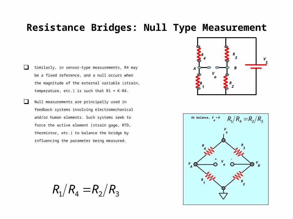
Resistance Bridges: Null Type Measurement
Similarly, in sensor-type measurements, R4 may be a fixed reference,
and a null occurs when the magnitude of the external variable (strain,
temperature, etc.) is such that R1 = K·R4.
Null measurements are principally used in feedback systems
involving electromechanical and/or human elements. Such systems
seek to force the active element (strain gage, RTD, thermistor, etc.) to
balance the bridge by influencing the parameter being measured.
3241 RRRR
B
VS
R2
R3
R4
R1
AV
o
At balance, Vo
= 0
Vs
R3
R4
R1 R
2
Vo
+ -
3241 RRRR
VB
VA
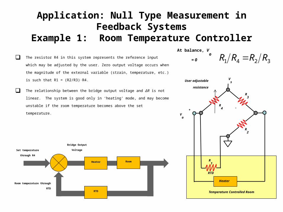
Application: Null Type Measurement in Feedback SystemsExample 1: Room Temperature Controller
At balance, Vo
= 0
3241 RRRR
Vs
R3
R4
RTD
R2
Vo
+-
Heater
Temperature Controlled Room
R1
The resistor R4 in this system represents the reference input which may be adjusted by the user.
Zero output voltage occurs when the magnitude of the external variable (strain, temperature,
etc.) is such that R1 = (R2/R3)·R4.
The relationship between the bridge output voltage and ΔR is not linear. The system is good only
in ‘heating’ mode, and may become unstable if the room temperature becomes above the set
temperature.
Set temperature through R4
Room temperature through RTD
Bridge Output
Voltage
Heater Room
RTD
User adjustable
resistance
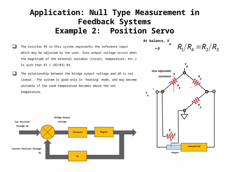
Application: Null Type Measurement in Feedback SystemsExample 2: Position Servo
At balance, Vo
= 0
3241 RRRR
VB
R3
R4
Magnet
R2
Vo
+-
R1
The resistor R4 in this system represents the reference input which may be adjusted by the user.
Zero output voltage occurs when the magnitude of the external variable (strain, temperature,
etc.) is such that R1 = (R2/R3)·R4.
The relationship between the bridge output voltage and ΔR is not linear. The system is good only
in ‘heating’ mode, and may become unstable if the room temperature becomes above the set
temperature.
Set Position through R4
Current Position through R1
Bridge Output
Voltage
Solenoid Magnet
R1
User adjustable resistance
Solenoid Coil
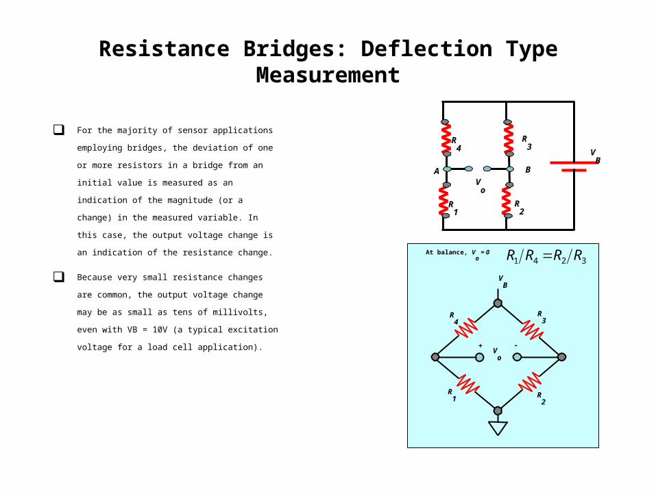
Resistance Bridges: Deflection Type Measurement
For the majority of sensor applications employing bridges,
the deviation of one or more resistors in a bridge from an
initial value is measured as an indication of the magnitude
(or a change) in the measured variable. In this case, the
output voltage change is an indication of the resistance
change.
Because very small resistance changes are common, the
output voltage change may be as small as tens of
millivolts, even with VB = 10V (a typical excitation voltage
for a load cell application).
B
VB
R2
R3
R4
R1
AV
o
At balance, Vo
= 0
VB
R3
R4
R1 R
2
Vo
+ -
3241 RRRR
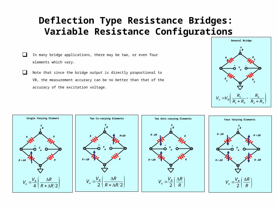
Deflection Type Resistance Bridges: Variable Resistance Configurations
In many bridge applications, there may be two, or even four elements which vary.
Note that since the bridge output is directly proportional to VB, the measurement accuracy
can be no better than that of the accuracy of the excitation voltage.
VB
R3
R4
R1 R
2
Vo
+ -
General Bridge
32
2
41
1
RR
R
RR
RVV Bo
VB
RR
RR + ΔR
Vo
+ -
24 RR
RVV Bo
VB
R+ΔRR
RR + ΔR
Vo
+ -
22 RR
RVV Bo
Single Varying Element Two Co-varying Elements
VB
R
RR + ΔR
Vo
+ -
R - ΔR
R
RVV Bo 2
Two Anti-varying Elements
VB
R + ΔR
Vo
+ -
R
RVV Bo 2
Four Varying Elements
R - ΔR
R - ΔR
R + ΔR
Deflection Type Resistance Bridges: Variable Resistance Configurations
In each case, the value of the fixed bridge resistor, R, is chosen to be equal to the nominal
value of the variable resistor(s). The deviation of the variable resistor(s) about the nominal
value is proportional to the quantity being measured, such as strain (in the case of a strain
gage) or temperature ( in the case of an RTD).
VB
R3
R4
R1 R
2
Vo
+ -
General Bridge
32
2
41
1
RR
R
RR
RVV Bo
VB
RR
RR + ΔR
Vo
+ -
24 RR
RVV Bo
Single Varying Element
VB
R+ΔRR
RR + ΔR
Vo
+ -
22 RR
RVV Bo
Two Co-varying Elements
VB
R
RR + ΔR
Vo
+ -
R - ΔR
R
RVV Bo 2
Two Anti-varying Elements
VB
R + ΔR
Vo
+ -
R
RVV Bo
Four Varying Elements
R - ΔR
R - ΔR
R + ΔR
Deflection Type Resistance Bridges: Single Varying Element Configurations
The single-element varying bridge may be used for temperature sensing using
RTDs or thermistors. This configuration is also used with a single resistive strain
gage. All the resistances are nominally equal, but one of them (the sensor) is
variable by an amount ΔR.
The relationship between the bridge output and ΔR is not linear. Since there is a
fixed relationship between the bridge resistance change and its output,
software can be used to remove the linearity error in digital systems.
Alternative bridge configurations can also be used to linearize the bridge output
directly.
VB
RR
RR + ΔR
Vo
+ -
24 RR
RVV Bo
Single Varying Element
Deflection Type Resistance Bridges: Two Co-varying Elements Configurations
In this configuration, both elements change in the
same direction. The nonlinearity is the same as that of
the single-element varying bridge, however the gain is
twice that of the single-element varying bridge.
The two-element varying bridge is commonly found in
pressure sensors and flow meter systems.
VB
R+ΔRR
RR + ΔR
Vo
+ -
22 RR
RVV Bo
Two Co-varying Elements
Deflection Type Resistance Bridges: Two Anti-varying Elements Configurations
This configuration requires two identical elements that vary in
opposite directions. This could correspond to two identical strain
gages: one mounted on top of a flexing surface, and one on the
bottom.
Such a configuration could be used for measuring force, pressure,
stress, strain, etc. It produces a linear is output, and it has twice the
gain of the single-element configuration.
VB
R
RR + ΔR
Vo
+ -
R - ΔR
R
RVV Bo 2
Two Anti-varying Elements
R - ΔR
R + ΔR
F
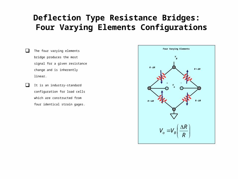
Deflection Type Resistance Bridges: Four Varying Elements Configurations
The four varying elements bridge produces
the most signal for a given resistance change
and is inherently linear.
It is an industry-standard configuration for
load cells which are constructed from four
identical strain gages.
VB
R + ΔR
Vo
+ -
R
RVV Bo
Four Varying Elements
R - ΔR
R - ΔR
R + ΔR
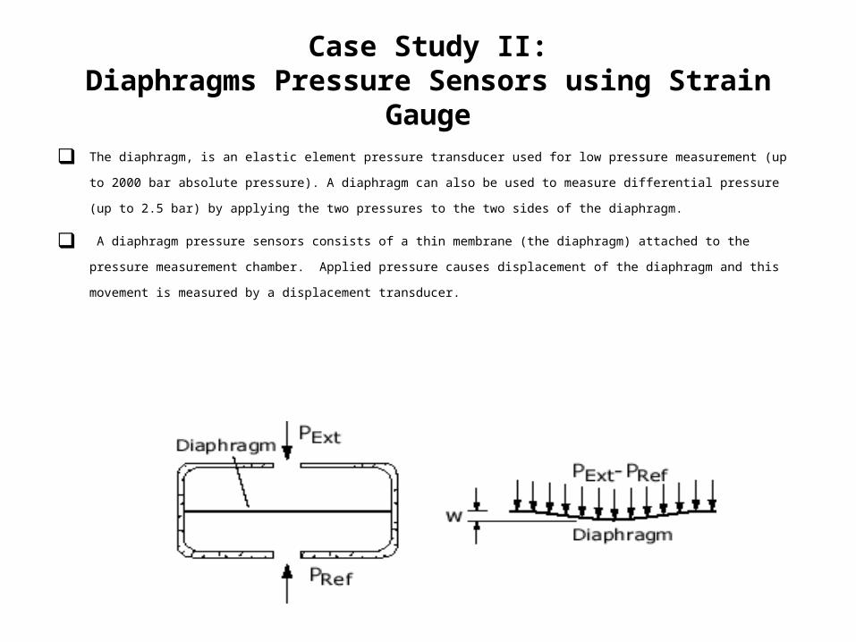
Case Study II:Diaphragms Pressure Sensors using Strain Gauge
The diaphragm, is an elastic element pressure transducer used for low pressure measurement (up to 2000 bar absolute pressure). A
diaphragm can also be used to measure differential pressure (up to 2.5 bar) by applying the two pressures to the two sides of the diaphragm.
A diaphragm pressure sensors consists of a thin membrane (the diaphragm) attached to the pressure measurement chamber. Applied
pressure causes displacement of the diaphragm and this movement is measured by a displacement transducer.

Case Study II:Diaphragms Pressure Sensors using Strain Gauge
The diaphragm can be either plastic, metal alloy, stainless steel or ceramic.
Plastic diaphragms are cheapest, but metal diaphragms give better accuracy.
Stainless steel is normally used in high temperature or corrosive environments.
Ceramic diaphragms are resistant even to strong acids and alkalis, and are used
when the operating environment is particularly harsh.
The typical magnitude of diaphragm displacement is 0.1 mm, which is well
suited to a strain-gauge type of displacement-measuring transducer, although
other forms of displacement measurement are also used in some kinds of
diaphragm-based sensors.
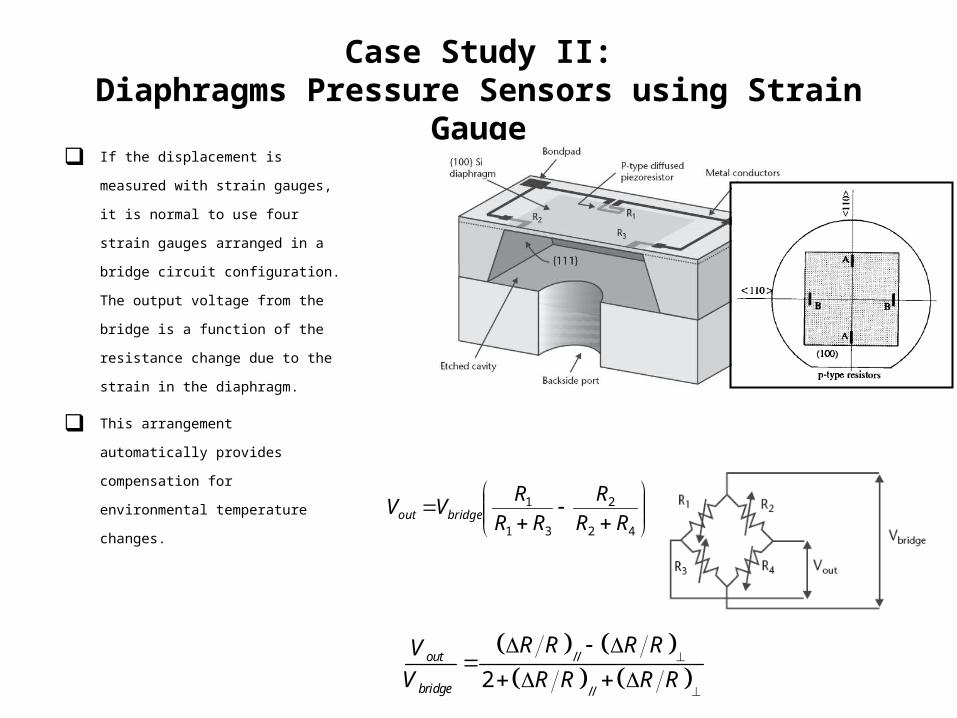
Case Study II:Diaphragms Pressure Sensors using Strain Gauge
If the displacement is measured with strain
gauges, it is normal to use four strain
gauges arranged in a bridge circuit
configuration. The output voltage from the
bridge is a function of the resistance
change due to the strain in the diaphragm.
This arrangement automatically provides
compensation for environmental
temperature changes.
42
2
31
1
RR
R
RR
RVV bridgeout
//
//2
out
bridge
R R R RV
V R R R R

Case Study II:Diaphragms Pressure Sensors using Strain Gauge
Older diaphragm pressure transducers used metallic strain gauges bonded to a diaphragm typically made of stainless steel. Apart from
manufacturing difficulties arising from bonding the gauges, metallic strain gauges have a low gauge factor, which means that the low output
from the strain gauge bridge has to be amplified by an expensive d.c. amplifier.
The development of semiconductor (piezoresistive) strain gauges provided a solution to the low-output problem, as they have gauge factors
up to one hundred times greater than metallic gauges. However, the difficulty of bonding gauges to the diaphragm remained and a new
problem emerged regarding the highly non-linear characteristic of the strain–output relationship.
42
2
31
1
RR
R
RR
RVV bridgeout
//
//2
out
bridge
R R R RV
V R R R R

Case Study II:Diaphragms Pressure Sensors using Strain Gauge
The problem of strain-gauge bonding was solved with the emergence of monolithic piezoresistive pressure transducers. These have a typical
measurement uncertainty of ±0.5% and are now the most commonly used type of diaphragm pressure transducer.
The monolithic cell consists of a diaphragm made of a silicon sheet into which resistors are diffused during the manufacturing process. Such
pressure transducers can be made to be very small and are often known as micro-sensors.
42
2
31
1
RR
R
RR
RVV bridgeout
//
//2
out
bridge
R R R RV
V R R R R

Case Study II:Diaphragms Pressure Sensors using Strain Gauge
Silicon measuring cells have the advantage of being very cheap to
manufacture in large quantities. Non-linear characteristic is normally
overcome by processing the output signal with an active linearization circuit
or incorporating the cell into a microprocessor based intelligent measuring
transducer. Such instruments can also offer automatic temperature
compensation, built-in diagnostics and simple calibration procedures. These
features allow measurement inaccuracy to be reduced to a figure as low as
±0.1% of full-scale reading.
By varying the diameter and thickness of the silicon diaphragms, silicon
diaphragam sensors in the range of 0 to 2000 bar have been made.
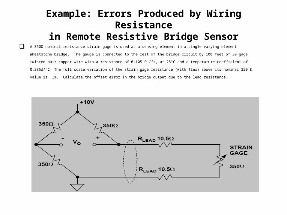
Example: Errors Produced by Wiring Resistancein Remote Resistive Bridge Sensor
A 350Ω nominal resistance strain gage is used as a sensing element in a single varying element Wheatstone bridge. The gauge is connected to the rest
of the bridge circuit by 100 feet of 30 gage twisted pair copper wire with a resistance of 0.105 Ω /ft, at 25°C and a temperature coefficient of 0.385%/°C.
The full scale variation of the strain gage resistance (with flex) above its nominal 350 Ω value is +1%. Calculate the offset error in the bridge output due
to the lead resistance.
Errors Produced by Wiring Resistancein Remote Resistive Bridge Sensor
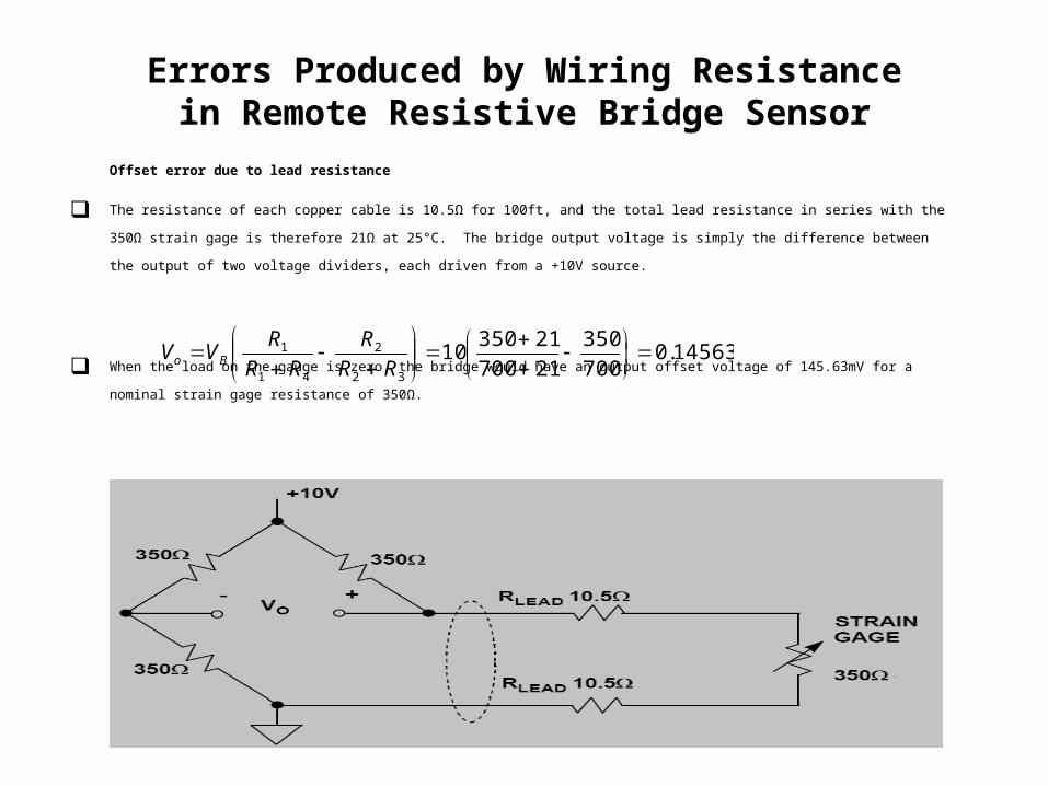
Offset error due to lead resistance
The resistance of each copper cable is 10.5Ω for 100ft, and the total lead resistance in series with the 350Ω strain gage is therefore 21Ω at 25°C. The
bridge output voltage is simply the difference between the output of two voltage dividers, each driven from a +10V source.
When the load on the gauge is zero, the bridge would have an output offset voltage of 145.63mV for a nominal strain gage resistance of 350Ω.14563.0
700
350
21700
2135010
32
2
41
1
RR
R
RR
RVV Bo
Errors Produced by Wiring Resistancein Remote Resistive Bridge Sensor
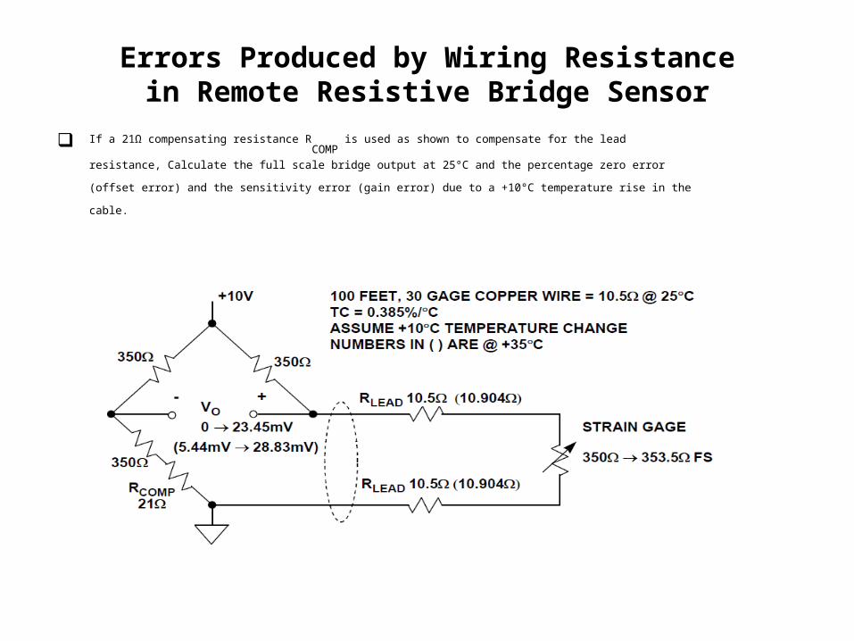
If a 21Ω compensating resistance RCOMP
is used as shown to compensate for the lead resistance, Calculate the full scale bridge output
at 25°C and the percentage zero error (offset error) and the sensitivity error (gain error) due to a +10°C temperature rise in the cable.
Errors Produced by Wiring Resistancein Remote Resistive Bridge Sensor
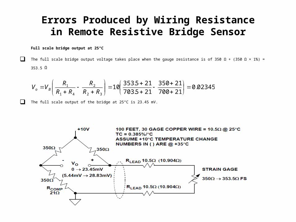
Full scale bridge output at 25°C
The full scale bridge output voltage takes place when the gauge resistance is of 350 Ω + (350 Ω × 1%) = 353.5 Ω
The full scale output of the bridge at 25°C is 23.45 mV.
02345.021700
21350
215.703
215.35310
32
2
41
1
RR
R
RR
RVV Bo
Example: Errors Produced by Wiring Resistancein Remote Resistive Bridge Sensor
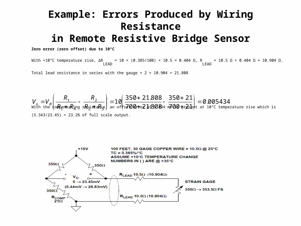
Zero error (zero offset) due to 10°C
With +10°C temperature rise, ΔRLEAD
= 10 × (0.385/100) × 10.5 = 0.404 Ω, RLEAD
= 10.5 Ω + 0.404 Ω = 10.904 Ω.
Total lead resistance in series with the gauge = 2 × 10.904 = 21.808
With the compensating resistance, an offset error of 5.434 mV is present at 10°C temperature rise which is (5.343/23.45) = 23.2% of full scale output.005434.0
21700
21350
808.21700
808.2135010
32
2
41
1
RR
R
RR
RVV Bo
Errors Produced by Wiring Resistancein Remote Resistive Bridge Sensor
Gain error due to 10°C temperature rise
The full scale bridge output at 35°C is calculated based on a gauge resistance of 350Ω + (350Ω × 1%) = 353.5Ω. The lead wire resistance, however, is (2
×10.904Ω = 21.808Ω
The full scale output due to 10°C temp rise is 28.83 mV giving a deflection from zero load of (28.83 - 5.434 = 23.396 mV) with an error of (23.396 –
23.45 = -0.054 mV) or (-0.054/23.45) = -0.23% of full scale output
02883.021700
21350
808.215.703
808.215.35310
32
2
41
1
RR
R
RR
RVV Bo
Errors Produced by Wiring Resistancein Remote Resistive Bridge Sensor
The effects of wiring resistance on the bridge output can be minimized by the 3-wire connection. The sense lead measures the voltage output
of a divider: the top half is the bridge resistor plus the lead resistance, and the bottom half is strain gage resistance plus the lead resistance.
Errors Produced by Wiring Resistancein Remote Resistive Bridge Sensor
The nominal sense voltage is independent of the lead resistance. When the strain gage resistance increases to fullscale (353.5W), the bridge
output increases to +24.15mV.
Errors Produced by Wiring Resistancein Remote Resistive Bridge Sensor
Gain error due to 10°C temperature rise
Increasing the temperature to +35ºC increases the lead resistance by +0.404W in each half of the divider. The fullscale bridge output voltage decreases to
+24.13mV because of the small loss in sensitivity, but there is no offset error. The gain error due to the temperature increase of +10ºC is therefore only –
0.02mV, or –0.08% of fullscale.