SCIENCES

DIVISION

INSTITUTE OF TECHNOLOGY

LIQUID GAS CYCLONE SEPARATION

by

Sanford Fleeter and Simon Ostrach

... •

U VERSITY CIRCLE • CLEVELAND, OHIO 0 U 1_96 °

few ̂

FrAS/TR-66-12

LIQUID GAS CYCLONE SEPARATION

by

Sanford Fleeter and Simon Ostrach

AFOSR Technical Report Nunber AFOSR 66-1400

June 1966

-■*■ »"T"*1" IW ' ■'''^■'-'^■«.l

ABSTRACT

This paper considers the secondary-flow of a liquid-gas

mixture in a cyclone separator. By means of a momentum integral

method, an engineering approximation to the secondary (heavy fluid)

flow rate is obtained which makes use of an experimental velocity

profile determined by ter Linden. This flow rate approximation is

physically realistic and is partially verified in the laboratory.

Tests were run on a separator to determine the effect of

the variation of certain operating conditions and geometric factors

on the separation of a liquid-gas mixture. Hie effect of these

variations on the efficiency of separation and pressure drop across

the separator as functions of the Reynolds and Weber numbers is

presented.

11

ACKNOWLEDO^ENTS

This research was made possible by the financial support

of the Air Force Office of Scientific Research (AF-AFOSR-194-66).

ill

TABLE OF CONTENTS

Page

ABSTRACT ii ACKNOWLEDGMENTS iii TABLE OF CONTENTS iv LIST OF FIGURES v. LIST OF TABLES V111

LIST OF SYMBOLS ix

CHAPTER I - INTRODUCTION

1.1 Cyclone Separation 1 1.2 Previous Work 4 1.3 Proposed Work And Relation To Previous Work 7

CHAPTER II - ANALYSIS

11.1 Derivation Of Boundary Layer Equations 9 11.2 Solution of Boundary Layer Equations 17 11.3 Boundary Layer Flow Rate 23

CHAPTER III - EXPERIMENT

I II.l Experimental Objectives 33 111.2 The Experimental Apparatus 35 111.3 Parameters 43 111.4 Results 45

CHAPTER IV - CONCLUSIONS 84

APPENDIX I Solution Of Boundary Layer Equations 86 APPENDIX II Experimental Data 91 BIBLIOGRAPHY 103

iv

LIST OF FIGURES

Figure Page

1 Cylindrical Section 1

2 Cyclone Configuration 3

3 The Stromquist Cyclone 5

4. The ter Linden Cyclone 6

5 Geodesic Coordinate System For Body of Revolution 12

6 Boundary Layer Velocity Profile and Approximation 20

7 Boundary Layer Thicknesses 22

8 Cone Exits For Boundary Layer Meeting 23

9 61/L1 vs. Lj 30

10 - Lj2 ECL^ vs. Lj 31

11 Heavy Fluid Flow Rate vs. ^ 32

12 Cyclone Dimensions 35

13 Schematic Diagram of System 38

14 Apparatus 39

15 Separator 40

16 Separator 41

17 Cone Tips 42

18 Separator 43

19 Efficiency vs. Reynolds Number for oil (v « 1.0) and Water for 15° Cone 47

20 Efficiency vs. Weber Number for oil (v « 1.0) and Water for 15° Cone 48

List of Figures (continued) Page

21 Pressure Drop vs. Reynolds Number for oil (v - 1.0) for 15° Cone 49

22 Pressure Drop vs. Weber Nunber for oil (v « 1.0) for 15° Cone 50

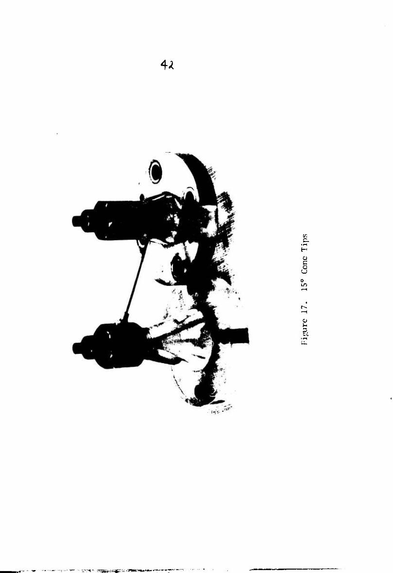
23 Efficiency vs. Reynolds Nunber for oil (v 1.0) at Various Heights for 15° Cone 53

24 Efficiency vs. Weber Number for oil (v ■ 1.0) at Various Heights for 15° Cone 54

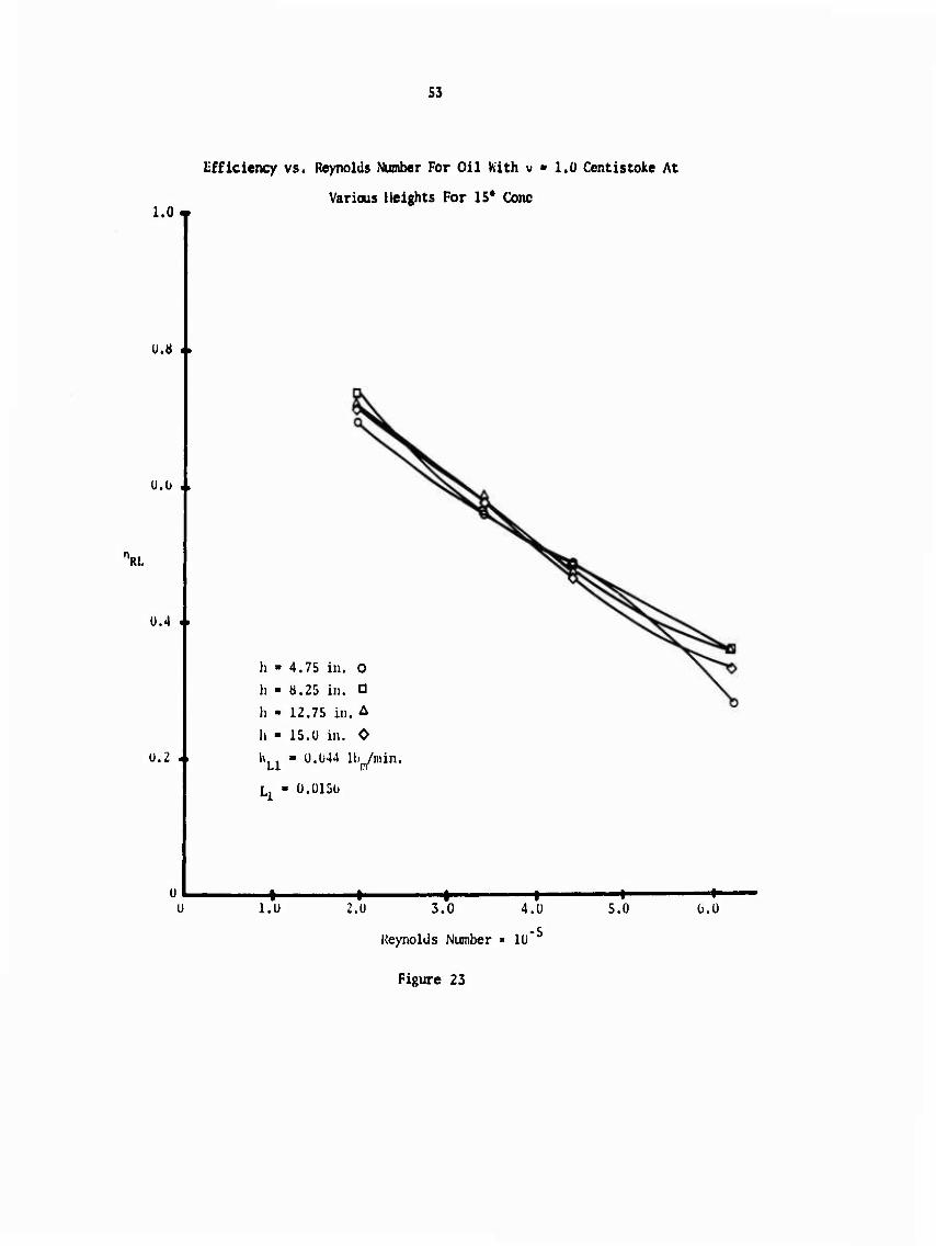
25 Efficiency vs. Reynolds Nunber for oil (v ■ 10) at Various Heights for 15° Cone 55

26 Efficiency vs. Weber Number for oil (v ■ 10) at Various Heights for 15° Cone 56

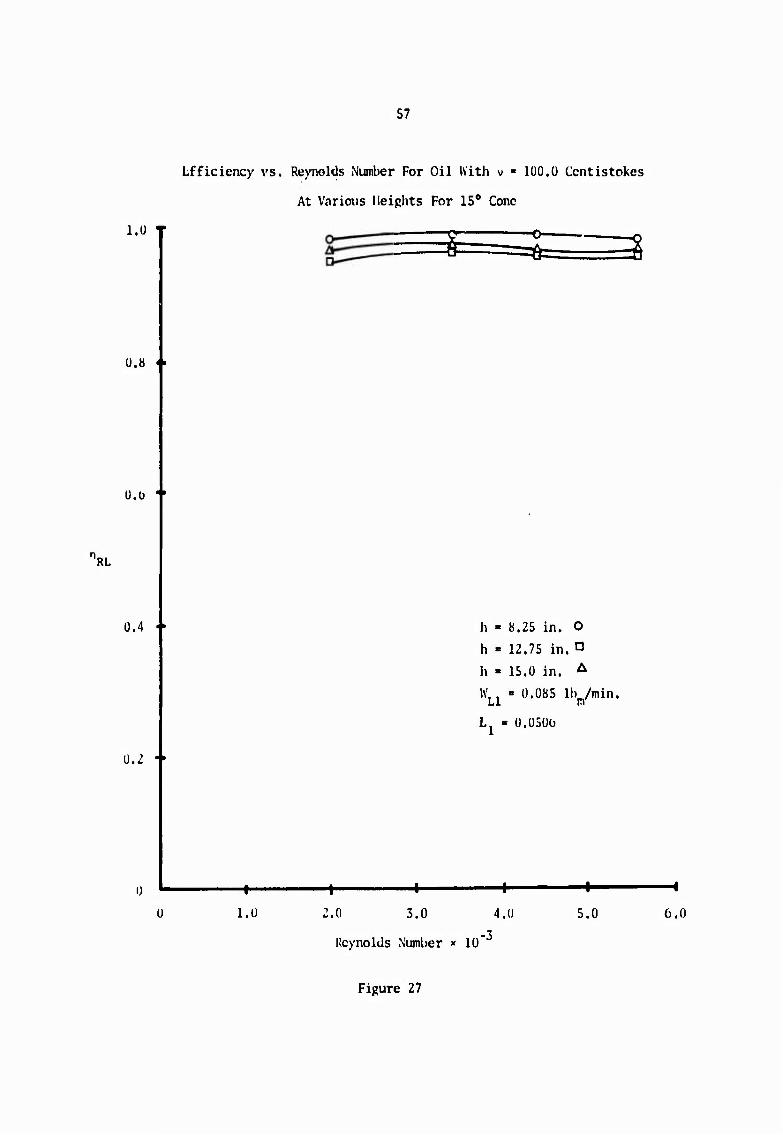
27 Efficiency vs. Reynolds Number for oil (v ■ 100) at Various Heights for 15° Cone 57

28 Efficiency vs. Weber Nunber for oil (v - 100) at Various Heights for 15° Cone 58

29 Pressure Drop vs. Reynolds Number for oil (v ■ 1) at Various Heights for 15° Cone 59

30 Pressure Drop vs. Weber Number for oil (v • 1) at Various Heights for 15° Cone 60

31 Pressure Drop vs. Reynolds Nunber for oil (v ■ 10) at Various Heights for 15° Cone 61

32 Pressure Drop vs. Weber Nunber for oil (v ■ 10) at Various Heights for 15° Cone 62

33 Pressure Drop vs. Reynolds Number for oil (v ■ 100) at Various Heights for 15° Cone 63

34 Pressure Drop vs. Weber Number for oil (v » 100) at Various Heights for 15° Cone 64

35 Efficiency vs. Reynolds Nunber for oil (v ■ 10) at Various Oil Flow Rates for 15° Cone 66

vi

List of Figures (continued) Page

36 Efficiency vs. Weber Number for oil (v ■ 10) at Various Oil Flow Rates for 15° Cone 67

37 Pressure Drop vs. Reynolds Number for oil (v » 10) at Various Oil Flow Rates for 15° Cone 68

38 Pressure Drop vs. Weber Number for oil (v ■ 10) at Various Oil Flow Rates for 15° Cone 69

39 Efficiency vs. Reynolds Number for oil (v ■ 10) at Various Underflow Diameters for 15° Cone 72

40 Efficiency vs. Weber Number for oil (v » 10) at Various underflow Diameters for 15° Cone 73

41 Pressure Drop vs. Reynolds Number for oil (v ■ 10) at Various Underflow Diameters for 15° Cone 74

42 Pressure Drop vs. Weber Nunber for oil (v » 10) at Various Underflow Diameters for 15° Cone 75

43 Efficiency vs. Reynolds Number for oil (v ■ 10) at Various Heights for 45° Cone 76

44 Pressure Drop vs. Reynolds Number for oil (v - 10) at Various Heights for 45° Cone 77

45 Efficiency vs. Reynolds Number for oil (v » 10) at Various Oil Flow Rates for 45° Cone 79

46 Pressure Drop vs. Reynolds Number for oil (v ■ 10) at Various Oil Flow Rates for 45° Cone 80

47 Efficiency vs. Reynolds Number for oil (v ■ 10) at Various Underflow Diameters for 45° Cone 81

48 Pressure Drop vs. Reynolds Number for oil (v » 10) at Various Underflow Diameters for 45° Cone 82

VI i

LIST OF TABLES

Table Page

1 Solution With K(x) - 13.6+26.1[sin(1.10x)e '^J 21

2 -L12 ECLj) vs. Lj 29

vm

k *.

U. S, IJEPARTMBNT GF Ca^ERCS ExpcrL-cntal Fora fc"l. Bureau of Public Roade

Report Kusbor:

Research and Development Studies ' 0379 * .'

/fflSTOACTItM AND EVAtUATICa l.v"tSnEBT

Report Title it Datet Stabilization of Silty Soils in Alaska, Part II, Interim Report

Author(s): E. R. Peyton and J. W. Lund

Program Area: D-3 (^651-0^2) Financing: (HPR-ra-Aaa.)*HER-l(2)

Conducting Agency: university of Alaska State Study Ident« Ko: 12^70

Sponsoring Agency: BPR Study Ident« Ko: 5 I 3 ] Year of a: [ ] year study

( x ) continuing

Project Status: Active (Approved, nctive, inactive, dropped, cc^pxe%cd or accepted)

1. Abstract: original by: D. G. Fobs Date: 1/27/66 edited or reviewed by: E. B. Kinter .Bate:

This brief interim report describes a laboratory study of the effects on the pcnr.3ability and frost heave characters sties of an Alaskan silt, AASHO Classification A-4(8), produced by adding Portland cement, tetra-sodium pyrophosphate (TSPP), tri-sodium phosphate, calcium chloride, and sodium hexametap&osphate. Frost heave tests vere performed to measure the effectiveness of polyvinyl membrane to prevent the detrimental effects of frost.

TSPP (0.3 percent) caused a large decrease in permeability and also proved most effective in reducing frost heave. Portland cement applied at rates from 1 to 3 percent did not greatly affect permeability and, for the soil tested, increased frost heave. The polyvinyl membrane prevented frost heave- but caused redistribution of tae water to the top of the specimen indicating the possibility of serious loss of strength in the upper layers of the pavement.

LIST OF SYMBOLS

A Cyclone Inlet Width

B Cyclone Inlet Weight

0 Cyclone Diameter

d Overflow Diameter

E Boundary Layer Velocity Parameter

?, Body Force per Unit Mass

p., F-, F3 Components of Body Force Vector in X, Y, Z Directions Respectively

f Underflow Diameter

F. Froude Number r K(x) Velocity Distribution

L Characteristic Length

L, Dimensionless X Coordiante of Heavy Fluid Exit (ratio of underflow diameter to cyclone diameter)

i-, X Evaluated at the Heavy Fluid Exit

P Pressure

p Dimensionless Pressure

cL Heavy Fluid Fow Rate in Boundary Layer

R Radius of Surface of Revolution

R Cyclone Radius

R Reynolds Number

\}fVtyi Velocity Components in X,Y, and Z, Directions Respectively

u,vyw Dimensionless Velocity Components

IX

List of Symobls (continued)

WÄ Weber Nunber e X Arc length along Generators of a Surface of

Revolution

Y Orthogonal Trajectories of Surface Generators

Z Coordinate Normal to the Surface of Revolution

x,y,z Dimensionless X^Y^Z, Coordinates

ß Inlet Angle

Y Dimensionless Body Force Vector

6 Boundary Layer Thickness

£ Dimensionless Boundary Layer Thickness

n Dimensionless Coordinate Normal to Surface in Boundary Layer

\L Efficiency of Removal of Heavier Fluid Components

e Semi-apex Angle of Cones

v Kinematic Viscosity of the Liquid

a Surface Tension of the Liquid

Page Line

2 4

9 13

14 11

15 19

17 3

17 11

27 6

37 19

51 8

70 2

78 9

ERRATA

Should Read

properly

subsequent

pressure

consideration 2

3u v 3u U 3X 3X W 3Z

Solution 61 1/2

value of .621 y-i- >.621 (Re) Ll

separator

23 and 24 with Figures 25 through 28.

(&! = f/d)

See Figures 37 and 46.

CHAPTER I

INTRODUCTION

1.1 Cyclone Separation

In the operation of a cyclone separator, a mixture, consist-

ing of either two fluids or a solid and a fluid, is introduced

tangentially into a cylindrical chamber. It is this tangential

injection which causes the mixture to enter into a vortex-like

motion which, in turn, produces a centrifugal force field. This

force field causes the heavier component of the mixture to move

outward - toward the surface of the cylinder. The lighter component

remains in the center portion of the cylinder. See Figure 1.

Cylindrical Chamber

X Injection Point

Boundary Layer

Figure 1

1

The initial concept of operation was that the heavier com-

ponent would exit downward only because of gravity, while the

lighter component would exit upward from continuity considerations.

Ostrach [1] indicated, however, that by a propely shaped exit for

the heavier component, e.g. a concial section, a secondary flow

would be generated. Ostrach based his concept on a generalization

of the work of Taylor [2] who showed that for the rotating flow of

a single fluid in a cone, secondary flows do exist. This rotational

flow together with the body force field determines the pressure

distribution in the boundary layer which, as discussed by Lawler [6]

and Taylor [2], is directed towards the apex of the cone. The

boundary layer fluid is retarded by viscosity and, therefore, does

not have sufficient inertia to maintain a circular path above the

cone axis. The pressure gradient then directs this retarded fluid

towards the cone apex where it exits.

Thus the discharge of the heavier component of a mixture in

a cyclone separator is the result of both gravity and a secondary

flow. The relative importance of this secondary flow is noted by

ter Linden who states that cyclone dust collectors have been

efficiently operated in an inverted position and by Lawler and

this author who operated a liquid-gas cyclone separator success-

fully, but not efficiently, in an inverted position. See Figure 2.

Lighter Component Exit

Gravity Boundary Layer

Heavier Component Exit

Figure 2

This operation of the cyclone separator in the inverted

position makes such a cyclone a possible means of delivering the

heavier component of the mixture to its exit in micro - or zero

gravitational environments. Also, the fact that a cyclone

separator has no moving parts makes it attractive for space appli-

cations.

1.2 Previous Work

This paper is concerned only with the case of liquid-gas

separation, that is, the case where a liquid is separated front a

mixture which is primarily gaseous. Therefore, in this section, a

review of only liquid-gas separation work is presented. For a com-

plete review of the work done on the other separation possibilities,

such as gas-gas, liquid-liquid, or gas-liquid, the reader is referred

to Lawler [6].

The principle analytical contribution to cyclone separation

is that due to Ostrach who described the discharge mechanism as

discussed in Section 1.1. Lawler, in his paper, assumed that the

flow in the conical section of the separator was that of a potential

vortex. A momentun-integral method was then used to predict secondary

flow rates. These predicted flow rates serve only as an upper bound

approximation, as noted by Lawler, because of two assumptions: (1)

The velocity of the outer edge of the liquid boundary layer is taken

to be the same as that of the inner rotating gas core; (2) The

flow can be represented by a potential vortex.

There exists a gaseous boundary layer between the inner gaseous

core and the liquid boundary layer. Hence the velocity of the outer

edge of the liquid boundary layer is lower than that of the inner

rotating gas core. A potential vortex flow implies that as the axis

of the separator is approached, the flow tends to infinity. In

actuality, however, the flow at the axis approaches a large but finite

velocity. Thus, in Lawler's approximation too large a value for the

velocities both at the axis of the separator and at the outer edge

of the fluid boundary layer have been assumed, leading to an upper

bound predicted flow rate.

Stromquist [1] experimentally investigated the effect of

varying the inlet flow rate and mass fractions of the components

of the mixture on a separator of fixed geometry. Data are presented

for both pressure drop and efficiency of removal. These data are

of questionable value as there were two design limitations: (1)

there was a guide vane normal to the surface of the separator;

(2) the heavy ccmponent exit was located on the side of the cone

near the apex (see Figure 3).

Figure 3. The Stromquist Separator

Van Dongen and ter Linden [4] in a somewhat qualitative

analysis, suggest that the concial section is not always the most

desirable shape due to turbulent re-entrainment of the liquid in

the strong secondary gas flows. They also speculate that a smaller

pressure drop would result for the separator shape indicated in

Figure 4.

A

V w\

T

'♦

Figure 4. The ter Linden Cyclone

Lawler, with the separator configuration indicated in Figure

2, used water and air as the working fluids to obtain data on pressure

drop and efficiency. However, the evaporation of the water into the

air and the fact that the Reynolds number could only be varied by

changing the inlet flow rate indicated the necessity of more experi-

mental infonnation.

1.3 Proposed Work And Relation To Previous Work

There are two primary purposes of the present study. The first

is to obtain analytically a more accurate engineering approximation

to the secondary flow rate. This is accomplished by an analysis

similar to those of Ostrach, Taylor and Lawler, but which makes use

of a cyclone boundary layer velocity profile which was experimentally

determined using dust particles in a gas by ter Linden [3]. This

analysis should result in more accurate secondary flow rate predictions

than those obtained by Lawler since the singularity of the potential

flow in the cylinder resulting from Lawler*s assumption of a potential

vortex has been eliminated. However, the effect of the gaseous bound-

ary layer on the velocity of the liquid boundary layer still has not

been considered. Hence, one might expect that this new secondary

flow rate prediction might still be too large.

The second purpose is to obtain improved experimental results,

making use of the same cyclone separator as used by Lawler. Over

certain ranges of operating conditions Lawler's working fluids,

air and water, may not have formed a mixture. Thus, it is desired

8

to improve the mixing of the two working fluids so as to have a

uniform mixture entering the cylindrical chamber over all operating

conditions. Also, as mentioned in the previous section, Lawler's

experimental results were affected by evaporation and by the

limited range of Reynolds nunber variation. Hence, results without

the effect of evaporation and over a wide range of parameter

variation are also to be obtained.

CHAPTER II

ANALYSIS

II.l Derivation Of The Boundary Layer Equations

The tangential injection of the fluid mixture into the

cyclone separator and the subsequent separation into components

and secondary flow is to be considered, for the purpose of analysis,

to be composed of three distinct and separate operations: (1) the

establishment of the rotational flow; (2) the separation of the

mixture into components; (3) the flow of the components.

A vortex-like flow is established in the cylindrical section

of the separator due to the tangential injection of the fluid mix-

ture. This has been observed experimentally by ter Linden [3] and

by Lawler [6].

Assuming the separation process to be independent of the

subsquent flow of the two components is not completely correct.

However, if this assumption is not invoked then one must consider

the mixing and separation with the flow model being one of globules

of one component dispersed in the other component which acts as

the carrier fluid of the mixture. As pointed out by Lawler, it is

extremely difficult if not impossible, actually to solve this pro-

blem in such a manner. Hence, in order to obtain an approximate

solution to the problem, it is assumed that the separation process

is independent of the flow of the mixture components.

■*.

10

To continue this analysis the following asstmptions are

made:

i) The actual separation of the mixture into a

lighter and a heavier component occurs only

in the cylindrical section of the cyclone

separator. This permits the boundary layer

flow to be considered independent of the

separation process.

ii) The cross-section of the separator is as

indicated in Figure 2 — The heavier

component is on the surface of the conical

section and the lighter component is nearer

to the center of the separator, away from

the surface of the cone. This assumption has

been experimentally verified,

iii) There is only one component of the mixture

comprising the boundary layer, namely the

heavier component. This perjnits a one-fluid

boundary layer analysis to be used.

iv) The heavier component of the mixture has a con-

stant viscosity and is also incompressible.

v) Time-independence of the flow is also assumed,

that is, steady flow.

£kw

11

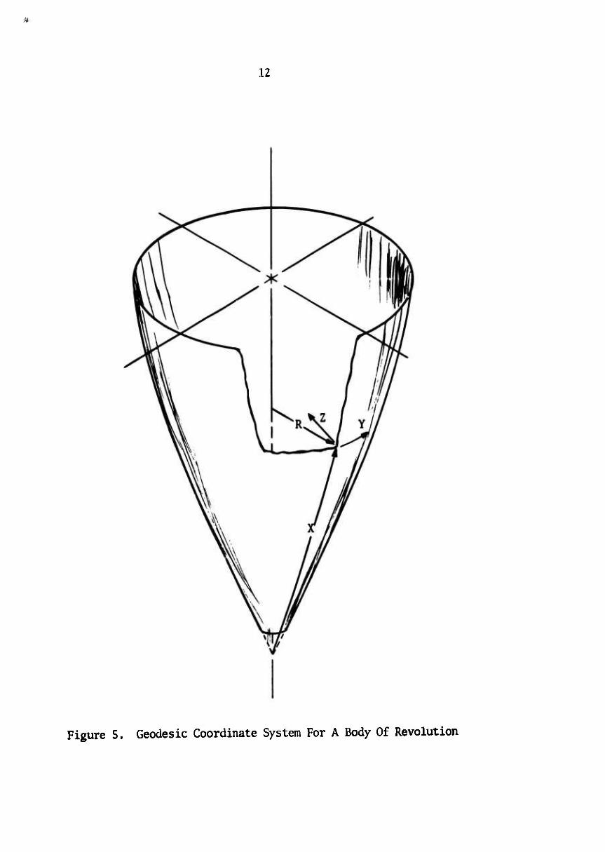
Next, a coordinate system must be chosen. A convenient

coordinate system to choose is the Geodesic Coordinate System as

suggested by Moore [5]. Another assumption is now made: the

surface under consideration is a surface of revolution with a

principal radius of curvature which is large compared to the

boundary layer thickness. This assumption permits the boundary

layer equations to be easily obtained in the Geodesic Coordinate

System. The reader is referred to Lawler [6] for the detailed

derivation of these equations.

In the Geodesic Coordinate System, the coordinates are de-

noted by X, Y and Z: X is taken to be the arc length along a

generator of the surface; Y is the azimuthal angle measured along

the orthogonal trajectories of the generators; and Z is the

normal to the surface. R, the radius of the revolution of the

generators, is a function of X which is specified for each particular

surface. Such a right-handed system is indicated in Figure 5.

The boundary layer and continuity equations in this coordinate

system are:

3ul "Z2 Dl , "2 3wl +

3wl . P 1 3P 3 wl n , , wi 3r"irR +ir Tr^iTT'h 'jw^-^i (2-la)

u, 3«2 A 3u,2 + 3u,2 + R' 1 3P 3 u2 n 1M

IT "37 + w3 -3l + wl -§X + U1W2 IT ,B F2 TIT 3Y + v -^1 ^"^

h~tiz-0 (2-lc)

12

Figure 5. Geodesic Coordinate System For A Body Of Revolution

.4..

13

Where Z is the velocity field whose components in the

X, Y and Z directions are respecti/ely w,» «,

and w,;

F,, F2 and F- are the respective components of the

body force per unit mass:

and R* denotes 2r *

In order to obtain non-dimensional equations, the inlet

velocity of the mixture, V , is chosen as a characteristic velocity,

and the following dimensionless quantities are defined:

X... _Y. .._Z...R x ziy^i z-r;r-L;

p wi w2 w3 p JU-«-iv-^r-;w-v-; pVJL ooo

o

Y. .-i.R ..JSLJF --2- (2-2) 1 || e v r L|

Where L is taken to be the length along the side of the

cone surface;

g is the acceleration due to gravity;

R , the Reynolds nunber, is the ratio of inertia

forces to viscous forces;

F , the Froude number, is the ratio of the inertia

14

forces to the body forces.

In non-dimensional form equations (2-la)- (2-Id) are:

2 2 au u 3li 3U V . 1 IP ... 1 3 U r* r^ u3x + r 3y + w3l""r IC7! "IT* IT 77 ^3a) e dz

., 3v * v v ^ 3v k uv . 1 1 iE. 1 32v (2-3b) 3x r y w 3z r PI T2 r 3y RÄ 7T r 6 oZ

i- Yj - |£ - 0 C2-3C)

?lx^+7l7#-0 ^

Looking at these equations and recognizing that the driving

force for the flow is composed of both the body force and the pres-

sure gradient, the relative importance of the Froude number can be

recognized. Since the Froude nunber multiplies only the body forces

and not the prssure gradient, the value of the Froude riunber

determines the relative importance of the two components of the

driving force: i) a small Froude nunber indicates that the driving

force will be primarily a result of the body force; ii) a large

Froude nunber indicates that the body forces will be but a negligible

part of the driving force. Hence, for large values of the Froude

number the body force terms may be neglected.

Two more assumptions are now made:

i) The only body force acting is that of gravity.

Also, the axis of revolution of the body is

15

parallel to the line of action of gravity.

This implies that y?18 0; Yi* + ^l-r'2 ;

Y,a r'. Thus, the shape of the underportion of

the separator determines the influence of the body

force in the X - direction. A suitable shape

could maximize or even eliminate the influence of

this body force component. For a conical under-

section, r' ■ constant and, for the special case

of R = L, a flat plate, r' = 1 and y = 0.

Hence a flat plate undersection would eliminate

the effect of body force in the X direction,

ii) Viscous flow theory states that the driving force

across a boundary layer is zero, that is,

Y, - ■£ ^ 0. Hence, by a consideration of the

inviscid flow outside of the boundary layer, the

pressure gradients within the boundary layer can

be determined.

The fact that the boundary layer flows over a surface of

revolution (a cone) can now be taken into consieration:

rj__ 1 r

-^ Geometry of a cone

TT- = 0 Axial symmetry of a cone.

16

Thus; the final boundary layer equations are:

ullUwiH.vi..3£+l A (2-4a) u ax w 32 x ax FT ^7 e dz

2

u a7+ w 3i+ -" r -i (2-4b)

^r'-||.0 (2.4c)

i^^-o-lx^*!?^ (2-4d>

To relate the driving forces within the boundary layer to

the outer inviscid flow, the Euler Equations and continuity must be

considered.

Let the subscript I denote the inviscid flow. Assume that

in the flow outside of the boundary layer u, = w, = 0.

2 Thus: \r]_ a 3£

X SS 3X

Equation (2-4a) becomes:

u|H .vi+v^=.!li+l 4 (2-5) 3x x 3z x K~ 7T K J

e dz

The boundary conditions for the boundary layer equations

2-5, 2-4b, 2-4c, 2-4d are:

u = v = 0 atz = 0 (2-6a)

u = 0 = |H = |X Vj = K(x) at z = 6 (2-6b)

where 6 is the boundary layer thickness; and v, « K(x) is

such that the inviscid flow may be said to be a

vortex-like flow.

II.2 Soultion Of The Boundary Layer Equations

In solving equations similar to the boundary layer equations

(2-4 )- (2-6 ), Taylor used a momentum integral method, integrating

from 0, the cone surface, to 6, the boundary layer thickness, with

respect to z..

In a manner similar to that of Taylor, equations (2-5) -

(2-4b,c,d) are integrated with respect to z from 0 to 6, giving

two integral relationships which must satisfy the boundary conditions

(2-6a) - (2-6b). The reader is referred to Appendix I for a

18

derivation of the integral relations. To satisfy the boundary

conditions let:

u - E(x) K(x) F(n) » E(x) K(x) (n-2n2+n3) (2-7a)

and 7 v - K(x) ♦(n) - k(x) (ZrvV) (2-7b)

where: n = —— = a dimensionless coordinate in the 6

direction normal to the boundary layer.

E(x) is a dimensionless parameter which allows

for changes in u with respect to x. E(x)

is to be determined.

K(x) determines the velocity profile in the bound-

ary layer and is assumed known.

These expressions, (2-7a) - (2-7b), are substituted into

the integral relations, and the variable of integration is changed

from z to n . The following two non-dimensional quantities are

defined:

Finally the integral relations are reduced to two differential 2 2 equations in terms of E and E6, with the condition that at x=l

corresportding to the outer edge of the cone— E = 6,» 0.

The final two non-linear differential equations are:

d ^ 3E2 „2 d r, „,.. 98 330 E2 n Q . cBc CE ) = - — " 5E cEc (ln KW) ■ — ■ ^JT (2"9a)

... -vtaftli

19

2

al (E6i J" 7 ir- + 7 E6i a^ ^n K(x)) + —r1-+ 285 (2-9b) xE

Taylor chose his K(x) to represent a potential vortex flow;

K(x) » n/R B ß/xsin0 where 0 is the semi-vertex angle of the cone

being considered. The corresponding dimensionless boundary layer

thickness is given by 61 = j^/j^ .

ter Linden experimentally determined the velocity profile

for dust particles in a cyclone separator of semi-vertex angle

equal to 15°. This author has approximated ter Linden's results

by K(x) « 13.6+26.1 [sin (l.lüx) e"0*95x]. See Figure 6. This

approximate velocity distribution is used herein for the numerical

solution of equations (2-9a) and (2-9b) in order to obtain a more

realistic secondary flow rate prediction. The results of the

numerical integration are presented in tabular form in Table I.

Figure 7, comparing the dimensionless boundary layer thick-

ness for K(x) equal to a potential vortex (Kx) ■ fl/R) and K(x) «

13.6 + 26.1 [sin (l.lOx) e'0,95x], indicates that for x close to

unity, the results are nearly the same whereas for the small x the

results differ. This result was to be expected due to the nature

of K(x) = 13.6 + 26.1 [sin (l.lOx) e'0,457] - chosen to be finite

at the origin as compared to the potential vortex which tends to

infinity for small x.

19.a

It should be noted that an exact calculation of the flow

characteristics in the separator would involve solving the two-fluid

problem, matching velocity and shear stress at the interface. Since

this is a very difficult problem, an approximate calculation was

used in this paper.

A better, but more involved, approximation would be the

following: first solve the single rotating fluid problem (for the

lighter fluid), imposing the no-slip condition at the separator sur-

face. Then evaluate the shear stress at the surface. Next, instead

of using the condition that at the outer edge of the heavier fluid

boundary layer the velocities of the two fluids are equal, use the

condition that the shear stresses are equal with the velocity gradient

of the lighter fluid at the interface being approximated by the

velocity gradient at the wall: ji| = Sr ^-^l^u •

This will yield a boundary layer thickness and velocity profilt

which could be considered to be the first step in an iterative scheme

to obtain a good approximation to the solution of the exact two-fluid

problem.

A.

2ü

28.0 -

24.U

20.0

10.ü

12.U ..

8.0

4.0

Velocity Profile and Approximation

— ter Linden's Hxperimental result

— Approximation

0 0.2 0.4 O.b 0.8 1.0

Figure 6

21

Solution with K(x) = 13.6 + Zö.lTsin (1.10x)e •0.95x.

x

-E

1.000 0.975 0.950 0.925 0.900 0.875 0.850

0.000 0.747 1.046 1.280 1.482 1.665 1.834

41 | 0.000 1.714 2.011 2.197 2.335 2.444 2.534

X 0.825 0.800 0.775 0.750 0.725 0.700 0.675

-E 1.992 2.143 2.289 2.429 2.567 2.702 2.837

61 2.610 2.676 2.734 2.784 2.828 2.865 2.896

X 0.650 0.600 0.550 0.500 0.450 0.400 0.350

-E 2.973 3.251 3.549 3.884 4.275 4.751 5.353

61 2.921 2.948 2.941 2.895 2.804 2.661 2.465

x 0.300 0.250 0.200 0.150 0.100 0.05 0.02

-E 6.150 7.254 8.88 11.48 16.22 27.81 54.17

2.215 1.915 1.575 1.210 0.835 0.462 0.221

Table I

22

Figure 7

23

11.3 Boundary Layer Flow Rate

For this section it is to be assumed that the boundary layers

meet at the apex of the cone. This means that only the boundary

layer flow consisting of the heavier component of the mixture will

be exiting through the cone apex. The reason for considering this

case is that the requirement of the meeting of the boundary layers

is one of the experimental operating criterion. The other

possibility — that of the boundary layers not meeting is discussed

in Lawler's paper [6].

For the ensuing discussion, which is still only concerned

with the flow in the conical portion of the separator, 0 is taken

as the semi-vertex angle of the cone, R is the radius of the cone

taken at its base, r,, is the exit radius and L, the characteristic

height is taken as the slant height of the cone.

Figure 8

24

As can be seen from Table I, the boundary layer equations

have been solved for small values of x. Physically, however, small

values of x correspond to the region near the cone apex, a region

in which the boundary layer may not be thin as compared to the

radius of curvature. Hence, the following assumption is necessary:

assume the results of the boundary layer analysis as

previously determined give a reasonable approxi-

mation to the flow for the region of small x.

The geometrical condition for the boundary layers to meet is:

6 ■ r^cosG = A,sin0 cose (2-10)

The volume flow rate in the boundary layer, dL is given by:

^H

rl 2nr u dr cosG (2-11)

r,-6/cos0

In order to use ter Linden's experimental results, equation

(2-7a) is used here to define u:

u - E(x)F(n)K(x) = E(x)K(x)(n-2n2+n3)

where n = T (2-12) Q

and K(x) = 13.6 +26.1 [sin(l.lOx) e"1^]

Note that the range of n is from 0 to 1, where n = 0

corresponds to the surface of the cone (r = r-.) and n = 1 represents

the outer edge of the boundary layer (r = r, -6/cos0).

(r,-!-) cose n= J 6

25

or -r = M COS0

TTius -dr cosG dn

Revnriting equation (2-11) in terms of n:

% ^nKEör, 2 3

(n-2n +n ) n6 r^cos© -1 dn (2-13)

Integrating and evaluating equation (2-13) ^ives the boundary

layer flow rate:

%

-nK(x)E(x)6r]

30 S- 26

r,cos0 (2-14)

From the physical criterion of the boundary layers being X

required to meet at the exit, Q * 1 :

qH = -0.314 K(x) E.(x) 6(x) ^ (2-15)

6 can be replaced by ^sinG cosG and r, by l^sine.

Also let £,« L L, where L, is the dimensionless X coordinate.

26

Note h rl 2rl that L, = -T- =g- =^2E"" . Hence L, can also be interpreted

as the ratio of the cone exit diameter to the maximum cone diameter,

as well as being the dimensionless X coordinate.

Then:

qH « -0.314 K(i1) EUj) L2!^2 sin 0 cose

K(OL Defining the Reynolds Number as R = :

c^ » -0.314 v RgE^2 L sin2e cos0 (2-16)

Note that R , L,, and 0 are all inter-re la ted fron the re-

quirement of having the boundary layers meet at the cone exit —

equation (2-10). Fran this equation and the expression for the

dimensionless boundary layer thickness, 6,:

6 = i, siTi0 cos0 * AT fii j-rr

L61 r^- or 6 = 4, sin0 cos0 ■ Msin0 JR" N

* e

i 1 61L

JsinO cos0 = ^ -4- (2-17) K l

rr— 1 6l or Jsine cos0 - --A (2-18) K l

27

61 To make use of equation (2-18), -r- is a function of L, ^ ll l

which has already been nunerically determined from the boundary

layer solutions. Hence equation (2-18) is actually a relationship

between L,, 0 and R which must be satisfied for the boundary layers

to meet. Since the left hand side of equation (2-18) has a maximum *1 1 1/2

value of one, then r" * T ^Re^ means that it is impossible

for the boundary layers to meet. To obtain the heavy fluid flow

rate, cL, equation (2-18) must be used in conjunction with equation

(2-18).

To facilitate the calculations of the boundary layer flow

rate, qH, the values of 61/L1 *** Ll2 ^ as f^tions of 4

are tabulated in Table II.

Figure 11 compares the heavy fluid flow rate as a function

of the dimensionless X coordinate, L,, for K(x) = a potential vortex,

and K(x) » 13.6 + 26.1 [sin(1.10x)e •:"A]. The secondary flow rate

predicted by means of a potential vortex appears to be physically

unrealistic since as L, tends to zero, the flow rate goes toward

infinity. This implies that as the cone exit diameter decreases

(L-jcan be expressed as the ratio of cone exit diameter to maximun

cone diameter) the flow rate increases.

Physically one might expect that as the exit diameter decreased

to zero, the out flow would also approach zero and, since for the

case of no cone (1^= 1) there would be no pressure gradient driving

the flow, there should also be no flow. This implies that there

J^

28

could exist a maximum flow rate.

Qualitatively the prediction presented herein based upon

K(x) - 13.6 + 26.1 [sin(l.lOx) e"0-95x] appears to be physically

realistic: as the exit diameter,L1, tends toward zero, so does the

flow; at Li = 1 (the case of no cone) the flow is zero; there

is a maximum secondary flow rate; a lower flow rate is predicted

than for the case of a potential vortex.

It is important that the reader be aware of the limitations

of these secondary flow rate equations. The equations cannot

distinguish the quantity of mixture entering the separator. Hence,

whether a large or a small quantity of mixture is introduced into

the cyclone separator, the same secondary flow rate will be pre-

dicted. Thus, in predicting the flow rate, not only must the con-

ditions of equations (2-16) and (2-18) be met, but also the predicted

outflow rate must not be greater than the inflow rate.

For the case of very small exit diameters (very small L,)

it would seem that the secondary flow rate should not be much

affected by the amount of fluid entering the separator. A very small

exit should imply that only a small quantity of liquid can be re-

moved. Figure 11 indicates the experimental points which appear

at lower outflow values than those predicted. This seems reasonable

when one recalls the assumption made in the analysis; the velocity

at the outer edge of the liquid boundary layer is the same as that

of the inner rotating gas core.

29

-Ll TKI^) vs. Lj

4-^ 1.00 0.9 0.8 0.7 0.6 0.5

-Eap 0 1.48 2.14 2.70 3.^b j.88

ö^Lj) 0 2.33 2.68 2.87 2.95 2.90

6l/Ll 0 2.59 3.35 4.10 4.92 5.80

-L^ECLj) 0 1.20 1.37 1.32 1.17 0.97

4-^ 0.45 0.40 0.35 0.30 0.25 0.20

-ECLj) 4.28 4.75 5.35 6.15 7.25 8.88

«iCLp 2.80 2.66 2.47 2.22 1.92 1.58

6l/Ll 6.22 6.65 7.06 7.40 7.68 7.90

-L^ECL^ 0.88 0.76 0.65 0.55 0.45 0.36

Ll IT 0.15 0.10 0.05 0.03 0.02 0.01

-EC^) 11.48 16.22 27.81 40.28 54.17 95.78

MV 1.21 0.84 0.46 0.31 0.22 0.12

6l/Ll 8.08 8.40 9.20 10.30 11.00 12.00

-L^ECLj) 0.26 0.16 0.070 0.036 0.022 0.010

Table II

3U

&l/l

12.0 «1

1Ü.Ü i

8.Ü

/U

U.2 Ü.4 O.b 0.8 1.0

Figure 9

31

1.4*

1.2

l.U

0.8

•Ljiap

U.t)

0.4

0.2

•L^Ldp vs. Lj

U.2 0.4 U.ü 0.8 1.0

Figure 10

4,<

3

24

lü.üüü . 8

0

l.UUO 8

0 .,

c E 1()U

&_ „

10

32

Heavy Fluid Tlow Rate vs. Lj

— -»Potential Vortex

—Approximation

O l.xperüiiental Points. « = 1U.U

U,4 o.o 0.8 1,0

Figure 11

CHAPTER III

EXPERIMENT

III.l Experimental Objectives

In Lawler's experiments a water-air mixture was injected in-

to the separator. This use of water and air as the working fluids

leads to the following three comnents pertaining to his results:

1) To form a water-air mixture, water was sprayed into

a moving stream of air. However, over certain

operating ranges, it appeared as though the water

spray «imply traveled down the inlet tube as a jet,

without mixing with the air, and impinged upon the

back-plate of the cylinder. This was due, to a

large extent, to the fact that the surface tension

of water is relatively high, 72 dynes/cm.

2) His results pointed out the necessity of obtaining

data without the effect of evaporation.

3) The Reynolds nunber could be varied only by varying

the inlet velocity of the mixture.

Air was still used as a working fluid due to its availability

but, to overcome the above limitations, silicone oils of different

viscosities were used in place of water. These oils were chosen

for the following reasons:

1) It was believed that they would not evaporate in air;

33

.K

34

2) Their surface tension was much lower than that of

water, approximately 20 dynes/cm. as compared to

72 dynes/cm. Hence, there should be a finer, more

uniform, oil spray which should mix easily with the

air stream and result in a more uniform mixture over

all operating ranges, eliminating impingement on

the back-piate.

3) Since a large number of silicone oils are readily

available with different values of kinematic vis-

cosities (but approximately the same value of sur-

face tension) the Reynolds hunber could be varied

independent of the inlet air flow rate.

Thus, for this study, air and silicone oils are used to

determine th^ Elects of varying the operating conditions and geo-

metric dimensions for the process of cyclone separation over a

relatively wide range of Reynolds number.

SS

III.2 The Experimental Apparatus

36

The dimensions of the separator used in this investigation,

the same separator as was used by Lawler, are indicated in Figure

12. It is made of cast acrylic and consists of a square cross-

section entrance section (A = B = 1.75 in.), an inlet angle ß

equal to 180°, a height, h, of 4.75 in. and a diameter, (2R0), of

4.5 in. The dimensions of this section are fixed throughout the

experiments, thus fixing the diameter of the cyclone. To this

basic unit of the separator, various overflow and underflow sections

can be attached.

The overflow section consists of a flat circular plate which

holds a cast acrylic overflow tube of diameter, d, of 1.75 in. and

overflow height, s, of 3,5 in. Because Lawler found that no effect

was produced by varying either d or s, these two conditions were

fixed during these experiments.

To the other end of the basic section it is possible to

attach either the underflow sections to be studied, or additional

cylindrical sections of diameter 4.5 in. also made of cast acrylic.

These additional sections make it possible to vary both the

cylindrical height, h, and the overall separator height H. The

range of variation of h was from 4.75 in. to 15.0 in.

The underflow section was chosen to be a cone so that the

theory might be verified. Two cone angles, 0, were used: 0 « 15°

and 0 = 45°. The apex of each of these acrylic cones was removed

so that various values of, f, the boundary layer flow exit diameter,

could be tested. For these experiments f varied from 0.052 in.

37

to 0.228 in. which correspond to ratios of exit diameter to

cyclone diameter (f/D) ■ £, from 0.015 to 0.05.1. For a cone, these

ratios represent the dimensionless x-coordinata of the boundary

layer fluid £,.

A schematic diagram of the experimental apparatus is shown

in Figure 13, while photographs of the system are shown in Figures

14 through 17.

The air flow was supplied by a Roots blower, varied by

means of a system of two bleed-off values, and measured by means

of an orifice meter. The volume flow rate of air was able to be

varied fron 0 to 138 cfm, corresponding to an inlet air flow rate

of from 0 to 100 fps.

The oil flow was obtained by using an oil accumulator,

charged with air pressure, to supply oil to calibrated spray

nozzles. The nozzles had to be re-calibrated for each of the

three silicone oils used (kinematic viscosities of 1, 10 and 100

centistokes).

The rate at which the boundary layer fluid left the

separater, the underflow rate, was determined fron a measurement

of the time required for a certain volune of the fluid to

accumulate.

38

"T

I 4)

rH N M o z

^

( fc-uwi-.i I

8. •H 4J

0^

JC=H^HH]

o CO

•*

'ti

O I

ft) rH

*

r^

vy

Bk

D ea

W I •H <

r-t

3*

3

4-* c

w

2 •H

*0

Figure 15. Cyclone Separator h = 8.25 in. e = 15{

i'.'iire l(). Cvclone Separator h 12.J!. in.

*r*mmm ■*■—

4^

O C o u

o

o

-,-.w--f.--^ ■'-L-*-*' .iraiii^wjK::^'*«»'««*^.».-

43

III.3 Parameters

(3) 'l Lighter Component Exit

(1) Mixture Inlet

Boundary Layer Flow lixit

Figure 18

The following parameters are used to evaluate the performance

of the cyclone separator.

i) The efficiency of removal, not, is defined as the

ratio of the mass flow of the boundary layer liquid

at the underflow, WL2, (Note: 1,2, and 3 refer to

Figure 18) to the mass flow rate of this fluid at

the inlet, W.,.

W L2

^ = ^Ll

When all of the heavier component is separated from the

mixture, the efficiency of removal will have the value of unity.

44

ii) The pressure drop is another, always important,

parameter which is considered.

iii) There are three similarity parameters

considfred: Reynolds nunber, Froude number and

Weber number. The Reynolds and Froude nunbers

were discussed in Chapter II and are given by

equation (2-2). The Weber nunber is defined

as the ratio of the inertia forces to the

cohesive forces, or surface tension, and is

given by

PV02L

e 2o

where a is the surface tension of the boundary

layer fluid.

Two criteria were established for the operation of this

separator: 1) there was no oil in the overflow (point 3 of

Figure 18) and 2) there was 100% oil in the underflow (point 2

of Figure 18). These two criteria are equivalent to demanding

100% purity of the air at the lighter component exit and 100%

purity of the oil at the heavier component exit.

For operation of the separator with the aid of gravity

criterion 2) was accomplished by placing a throttling valve at the

heavier component exit, while the violation of criterion 1) was

used to determine the end of a test run.

45

111.4 Results

The experimental results presented in the following graphs

indicate data points which have been averaged over three runs at a

given condition in which the variation was less than 21. Samples of

this data are presented in Appendix II.

The Weber number is varied only by changing the reference or

inlet, velocity. This is due to the surface tensions of all three

oils used, v ■ 1.0, 10.0, 100.0 centistokes, being approximately the

same, 17.4, 20.1, 20.9 dynes/cm. respectively. The advantage of

having a nearly constant value of the surface tension is that the

spray characteristics and, hence, the mixing is very nearly the same

for each oil.

The Reynolds number for each individual oil is varied by

changing the inlet velocity. However, the Reynolds number can also

be varied independently of the inlet velocity by changing the value

of the viscosity, i.e., using a different oil.

Figures 19 and 20 indicate the variation in efficiency, as

functions of the Reynolds number and the Weber number respectively,

for oil with v ■ 1.0 centistoke and water (v ■ 1.0 centistoke).

From these graphs it appears as though the oil may be evaporating into

the air stream at an even faster rate than for the water, and in fact,

that is what has happened. Placing equal masses (33.4 grams) of

water and oils with v « 1.0, 10.0, 100.0 centistokes into an air

stream for a short interval of time, it was found that 1.0 grams of

water, 2.2 grams of v = 1.0 oil, 0.2 grams of v - 10.0 oil and 0.0

46

grams of v - 100.0 oil, had evaporated. It should also be noted

that this test air stream was traveling with a velocity much lower

than that found in the separator. Hence, it is expected that these

evaporation effects would be even more pronounced in the cyclone

separator.

47

Efficiency vs. Reynolds Number For Oil (v ■ 1.0 Ccntistokc)

And Water For 15° Cone

1.0-

U.8,

0.0,

'RL

ü.4i

0.2

I120: WL1 = 0.053 lbm/min. 0

Oil: UL1 = 0.044 lbm/min. A

h » 8.25 in.

L - 0.0150 l

0.3 0.6 0.9

Revnolds Number * 10 -4

1.2 1.5

Figure 19

48

i.U T

Lfficiency vs. Kcber Number For Oil (v ■ 1.0 Centistoke) And

Ivatcr Por 15° Cone

U.8 ••

U.O

'RL

U.4

Ü.2

H20: \\ = U.Ü53 lbm/miii. O

Oil: V.,. =0.044 lb /min. A LI m

h = 8.25 in.

1^ = 0.0150

1.0 2.0 3.0

Weber Number x 10

4.0 5.0

Figure 20

49

Pressure Drop vs. Reynolds Number For Oil (v ■ 1.0 Centistokc)

And IVater For 15° Cone

24

2U

10

<s

i/i 12

b «•

4 ■-

H.O: WT1 = U.Ü53 lb /min. O 2 LI m

Oil: U, , = 0.U44 lb /min. A LI m

h = 8.25 in.

Lj^ «= Ü.U150

1.5

Reynolds Number * 10 -4

Figure 21

50

Pressure Drop vs. Weber Number For Oil (v ■ 1.0 Ccntistokc)

And Water For 15° Cone

24

2Ü

lo ■•

o

a, u si u

12

il20: WL1 - Ü.Ü53 lbm/min. O

WT1 = U.044 II) /min. A

LI m

b = 8.25 in.

L1 = 0.0150

Weber Number x 10 -5

Figure 22

51

First, the cone with semi-vertex angle equal to IS9 will

be discussed.

Figure 23 through 34 indicate the effect of the separator

height, h, on the efficiency of removal and the pressure drop across

the separator as functions of the Reynolds number and the Weber

number. The effect of the high evaporation rate of the v ■ 1.0 oil

as compared to the other oils is easily seen by comparing Figures

28 and 29 with Figures 30 through 34. For v « 1.0 oil, the efficiency

decreases with increasing inlet velocity, while for v » 10.0 and

v ■ 100.0 oils the efficiency remains nearly constant, at nearly

100% efficiency. It should be noted that the results of Lawler's

experiments exhibit the same effect as the v » 1.0 oil, efficiency

decreasing with increasing inlet velocity. Hence, Lawler's conclusion

that evaporation had a large effect upon his results appears to be

correct.

Increasing the separator height decreases the pressure drop

across the separator as can be seen from Figures 29 through 34.

This result agrees with that of Lawler. It can be explained by

realizing that at steady-state, the rate of energy input at a given

inlet velocity is constant, equal to the rate of dissipation. Thus,

increasing the height reduces the fluid's rotational speed so as to

maintain constant dissipation, and along with this reduced speed

goes the fact that it requires less of a pressure drop to support

the flow.

52

Due to the high evaporation r.ite, the oil with viscosity

v ■ 1.0 centistoke will not be considered in the remainder of

this paper.

S3

1.0«

Efficiency vs. Reynolds Number For Oil Kith v - 1.0 Centistoke At

Various Heights For IS* Cone

U.8

u.o

"RL

Ü.4

0,2

h • 4.75 in. 0

h - 8.25 in. a h - 12.75 in . A

h • 15.U in. 0

\l - Ü.Ü44 lb /min.

^ - o.oiso

—•- 3.0

—♦- 4.0 1.0 2.Ü 5.0 0.Ü

Reynolds Number « 10'

Figure 23

54

1.0'

Lfficiency vs. I'.eber Number For Oil With v ■ 1.0 Centistokc

At Various lieiglits for 15° Cone

Ü.8 +

ü.öt

'RL

Ü.4

0.2

= 4.75 in. O

= 8.25 in. n

= 12.75 in.A

= 15.Ü in. O

L1 = U.U44 lbm/min.

l1 = 0.0150

■4- ■4-

U.() 1.2 1.8 2.4 3.0

Ivcber Niunber »10

Figure 24

-5

SS

Efficiency vs. Reynolds Nunber For Oil With v - 10.0 Centi.-tokes

At Various Heights Fbr 15° Cone

'RL

1.0] •

-6. O-

U.8 , •

«^^

0.0 | i

Ü.4 i h ■ 4.75 in. o

h - Ö.25 in. D

h - 12.75 in. A

h - 15.ü in. 0

IV, , « 0.053 lb /min. LI m

U.2 • l1 • 0.0175

0 | 1 —1— l.U :.u 3.o

Reynolds Number « 10

4.0

-4

S.Ü 0.0

Figure 25

56

Efficiency vs. Weber Number For Oil With v ■ 10.0 Centistokes

At Various Heights For 15° Cone

1.0 T

U.b"

0.0'

'RL

0.4.

0.2'

h - 4.75 in. O

h - 8.25 in. Q

h - 12.75 in. A

h - 15.0 in. O

WL1 - 0.053 Ib^min.

ll ■ 0.0175

üL -•-

0.5 1.0 1.5

V.'cbcr Number »10

2.0

5

2.5 3.0

Figure 26

57

Lfficiency vs. Reynolds Number For Oil With v ■ 100.Ü Ccntistokes

At Various Heights For 15° Cone

1.Ü T 5 =6= '^

u.u

Ü.0

RL

0.4

Ü.2

-I—

l.U 2.0

h - 8.25 in. O

h ■= 12.75 in. °

h - 15.0 in. A

l\' » 0.085 lb /min. Li m

L1 - 0.0500

3.0 4.0 5.0

Reynolds Number * 10'

6.0

Figure 27

58

Efficiency vs. Weber Nimber For Oil With v - 100.0 Centistokes At

lg Various Heights For 15° Cone

2= ^ ' Ä Ä

U.8'

Ü.b.

"RL

Ü.4"

U.2.

h « b.25 in. O

h - 12.75 in. □

h - 15.0 in. ^

LI U.Ü85 Ibymin.

L, - Ü.U5Ü0

•4- 4- ■•-

U.4 Ü.8 1.2

Ueber Number « 10"

1.6

3

2.0 2.4

Figure 28

59

Pressure Drop vs. Reynolds Nunber For Oil With v - 1.0 Centistoke

At Various Heights For IS* Cone

24«

2U..

lö

<*4 o a i2.,

a. <

h ■ 4.75 in. o h ■ 8.25 in. a h - 12.75 in. A

h - 15.Ü in. O

W,. »0.044 lb /min. Ll It)

1^ ■ Ü.Ü15Ü

t- ■♦■

4.0

5

1.0 2.0 3.0

Reynolds Number * 10

5.0 6.0

Figure 29

60

Pressure Drop vs. Weber Number For Oil With v - 1.0 Centistokc

At Various Heights For 15° Cone

24«

20,,

lb..

CM

o V) o

<

12..

8 ..

4 ,,

h ■ 4.75 in. O

h • 8.25 in. n

h - 12.75 in.A

h - 15.0 in. O

W,. - 0.044 lb /min. Li m

- 0.0.150

0.6 1.2 1.8

Weber Number * 10 -5

2.4 3.0

Figure 30

61

Pressure Drop vs. Reynolds Number For Oil With v • 10.0 Centistokes

At Various Heights For IS* Cone

5.0' '

4.0<»

o

1/1

<3

3.Ü..

2.0.»

l.ü<.

h - 4.75 in. o

h - 8.25 in. D

h - 12.75 in. A

h - 15.ü in. O

IV - Ü.Ü53 Ity'min

Lj - Ü.Ü175

-•- ■+■ 1.Ü 2.Ü 3.0

Reynolds Number « 10

4.1)

-4

5.0 6.0

Figure 31

62

Pressure Drop vs. Weber Number For Oil With v ■ 10.0 Centistokes

At Various Height« For 15° Cone

5.Ü

4.0

5.0- . o

2.Ü

1.Ü

h ■ 4.75 in. O li ■ 8.25 in. D h - 12.75 in. A

h «= 15.0 in. O

IV., « 0.053 lb /min. m

Lj^ ■ 0.0175

—I- U.5 1.0 1.1 :.ü

Weber Number »10 ■.-5

3.0

Figure 32

63

Pressure Drop vs. Reynolds Number For Oil With v ■ 100.0 At Various

Heights For 15° Cone

3.5

3.0"

2.5

CM

^ 2.0' o

42

< 1.5

1.0'

0.5

h ■ 8.25 in.

h - 12.75 in.

h ■ 15.0 in. WL1 - 0.085 lb,

L - 0.0500

4- 4- —f- 4.0

3

1.0 2.0 3.0

Reynolds Number * 10'

5.0 6.0

Figure 33

64

c

m £

Pressure Drop vs. Weber Number For Oil Kith v ■ 10Ü.0 Centistokes

At Various Heights For 15° Cone

3.5.-

3.Ü,

2.5..

2.Ü ■.

^ 1.5

1.Ü

Ü.5

Ü.4 -f-

U.8 1.2

Weber Number «10

1.6

-5

2.U 2.4

Figure 34

65

The effect of varying the oil inlet flow rate on efficiency

and pressure drop is indicated in Figures 35-38. The efficiency

of removal increases with increasing oil flow rates, approaching

close to 100% efficiency at the higher flow rates. This may be

due to the fact that at a given air inlet velocity (indicated on

the graphs by a particular Reynolds or Weber number), the

evaporation rate is nearly constant, (a very small constant).

Thus, by increasing the oil flow rate, the fraction of oil which

is evaporated decreases, and the efficiency increases.

The pressure drop across the separator decreases slightly

with increasing oil flow rates at a particular Reynolds or Weber

number. This is seen in Figures 37 and 38. Lawler found this

same result which he felt was due to the speed of rotation of the

cyclone being reduced by the increased mass of oil in the separator

at the higher oil flow rates. The effect of the decrease of

rotational speed on the pressure drop was discussed earlier in

this paper.

66

Efficiency vs. Reynolds Nunber For Oil With v ■ 10.Ü Centistokes

At Various Oil Flow Rates For 15* Cone

l.ü f

Ü.8 •

O.b

'RL

U.4

Ü.2 ■

1.Ü 2.U

WL1 • U.053 Ihjmin. 0

WL1 - Ü.083 U^/min. D

lVLl - 0.114 Ib^min. A

li - 8.25 in.

L1 - Ü.017S

3.Ü 4.Ü 5.U b.O

Reynolds Number K lü"

Figure 35

b7

Lfficiency vs. Ueber Number For Oil With v ■ 1U.Ü Ccntistokes

At Various Oil Flow Rates For 15° Cone

1.Ü *

U.8 <»

U.o

'KL

U.4 i. " U.UW H /mil.. O

\\ = o.Utö Ib/inin. L;

Is., = 11. lit Hi /min. A LI m'

ij,*.J Hi,

Lj •= Ü.U17D

l.U 1.5

Weber Ntimher » 10

U.5 2.U

-5

3.U

Figure 3b

68

Pressure Drop vs. Reynolds Number Por Oil With v - 1U.U Centistokes

At Various Oil How Rates For 15° Cionc

3.Ü..

4.O.,

o

3.Ü

2.U,

1.0,

V.,, •= Ü.Ü53 lb /min. O LI m

l\L1 » Ü.U83 ll)m/inin. n

W,, = U.114 lb /min. ^ LI m'

li ■ 8.25 in.

L1 « U.U175

—^

1.Ü 3.'J 2.U

Reynolds Number « 1U

A.O

-•1

b.Ü b.Ü

l'igure 37

69

Pressure Drop vs. Weber Number For Oil With v - 10.0 Ccntistokes

At Various Oil Flow Rates For 15° Cone

5.Ü ■•

4.U

o = 3.U

o

2.0

1.0 ,,

K.. " 0.053 Hi/rain. O Li In

WT, « 0.083 lb /min. Q LI m

lvL1 » 0.114 U) /min. A

li ■ H.2J in.

L1 - 0.0175

-•- •+• U.5 1.0 1.5 2.0

hoher Number «10

Figure 38

:.5 3.0

70

Figures 39 through 42 indicate the effect of the under-

flow diameter Ui " fid) on efficiency and pressure drop. The

efficiency decreases as the underflow diameter increases. The

pressure drop across the separator is decreased slightly at high

Reynolds number as the underflow diameter is increased. This is

to be expected as an expansion of the underflow would decrease the

pressure drop. This agrees with Lawler's results.

This completes the presentation of the results of experiments

run on the 15° cone. Next consider the effect of varying operating

conditions and the Reynolds and Weber numbers on a cone of semi-

vertex angle of 45°. Only the oil with viscosity v ■ 10.0 centistokes

was used for these tests as the primary interest in these results

is as a comparison with the results for the 150cone.

Figures 43 and 44 indicate the effect of separator height

variation on the efficiency and pressure drop. It can be seen that

the efficiency decreases as the separator height increases, as for

the 15° cone. Comparing Figures 25 and 43 it appears as though the

efficiency is not much affected by the change in cone angles. The

45° cone results do exhibit a very slight increase in efficiency

over the 15° cone as can be seen by comparing Figures 25 and 43.

This increase agrees qualitatively with the theory which, indicates

2 that qH should be proportional to sin e* coso with all of the other

variables fixed. A more physical interpretation is that the

driving force, the pressure gradient toward the cone apex, increases

as the cone angle increases. Hence, the cone with the larger semi-

71

vertex angle is more efficient. Lawler found a marked increase

in the efficiency of the 45° cone as compared to the 15° cone.

However, he attributed this to the fact that the fluid's residency

time in the 45° cone was less than in the 15° cone, and therefore,

evaporation had less of an effect. Using oil with v * 10.0 centi-

stokes, there is not very much evaporation and, therefore, there

is less charge in efficiencies caused by using cones of different

angles. For the 45° cone, as for the 15° cone, the pressure drop

decreases with increasing height. This decrease, at a particular

Reynolds number, is much greater for the 45° cone than for the 15°

cone as can be seen by comparing Figures 31 and 44. This last

result agrees with that found by Lawler.

72

Lfficiency vs. Reynolds Number Por Oil With v ■ 10.Ü Centistokes

At Various Underflow Diameters For 15° Lone

1.Ü

U.B

U.O

RL

U.4

U.J

L. •= U.UISO O

L = 0.Ü1O2 D

L. « U.U17S A

V.' = Ü.U53 Ih /min. Li n'

li - ii.25 in.

l.U 2.0 3.Ü

I'eynolds Number « 10

4.0

4

5.0 O.O

Figure 39

73

Efficiency vs. Weber Number For Oil With v • 10.0 Centistokes At

Various Underflow Diametes For IS* Cone

l.UT

Ü.8«'

ü.b'>

'RL

U.4-.

U.3.

L - O.ülSb O

Lj - O.ülüZ □

Lj - Ü.0175 ^

W,. - 0.053 lb /min. LI m

h « 8.25 in.

U.5 —H 1 H-

1.0 1.5 2.0

Weber Number x lü"5

2.5 3.0

Figure 40

**.

74 Pressure Drop vs. Reynolds Number For Oil With v ■ 10.0 Centistokes

At Various Underflow Diameters For 15* Cone

5.Ü"'

4.Ü« h l^ - u.oiso o

l^ - ü.üio2 n

1^ ■ Ü.0175 A

3s U,. - Ü.Ü53 lb /min. Ll m

h - 8.25 in.

0 3.0' •

<

2.Ü

l.U

l.U 2,0 3.Ü

Reynolds Number »10

4.0

-4

5.0 b.O

Figure 41

75

Pressure Drop vs. Weber Number For Oil With v ■ 10.0 Centistokes

At Various Underflow Diameters For 15° Cone

S.Ü <-

4.Ü..

= 3.U

i/i

i.ü<

l.u.

L - U.U155 n 1

L = 0.U1O2 □ 1

L - U.Ü175 A l

l\,. « 0.055 11) /min. LI tn

0.5 -♦-

l.o i.S

l.elier Number « 1Ü

—H 2.0

5

2.5 3.0

Figure 42

k%

76

'RL

tfficiency vs. Reynolds Nunber For Oil With v 10.0 Centistokes

At Various Heights For 45° Cone

1.0-

0.8'

0.6

0.4

0.2

oL 1.0 2.0

h ■ 8.25 in. o

h - 12.75 in. D

h » 15.0 in. A

U' - 0.060 lb /min. Li m

L • 0.0175 l

3.0 4.0 5.0

Reynolds Number * 10 -4

Figure 43

77

Pressure Drop vs. Reynolds Number For Oil IVith v « 1Ü.Ü

Centistokes At Various Heights For 45° Cone

7 S 4# « «/

2.U

(SI

Ü

c

1.5

1.Ü

U.5 ..

li = Ü.25 in.

h = 12.75 in.

h = 15.U in.

IV = U.UUU lb,

L = U.U175 l

1.Ü 2.0 3.0 4.0 5.0

Reynolds Number x 10'

Figure 44

tk.

78

Figures 45 and 46 show that, for the 45° cone, the higher

the oil flow rate, the greater the efficiency and the smaller the

pressure drop. These are the same type of results as found for

the 15° cone. However, the curvatures of the pressure drop versus

the Reynolds nunber are different for the two cones: the 45° cone

results indicate that may be sane maximal pressure drop, that is,

some Reynolds number beyond which the pressure drop across the

separator is constant, whereas the 15° cone results do not indicate

the possibility of such a maximum. See Figures 36 and 46.

Figures 47 and 48 present the effect of underflow diameter

on efficiency and pressure drop. The efficiency tends to decrease

as the underflow diameter increases, as for the 15° cone. The

pressure drop, while large for the 45° cone also exhibits the

same trend as the 15° cone, decreasing as the underflow diameter

increases.

79

Lfficiency vs. Reynolds Number For Oil With v ■ 1U.Ü Ccntistokes

At Various Oil Flow Rates For 45° Cone l.U.

U.8

ü.b

'RL

0.4

U.2

o—

1.Ü :.ü

W, , = U.Ü57 lb /min. O LI m

VvL1 = (J.1U2 lbm/min. □

h = 8.25 in.

L = O.U175

3.U 4.Ü 5.Ü

I^eynokls Number * 1U

Figure 45

8U

CN

O

-3

Pressure Droj- vs. Refolds Niunbcr l:or Oil With v = 10.U

Centistokes At Various Oil Flow Rates For 45° Cone 7 5

2.0

1.5

l.U

U.5

■•-

l.U

h, , = U.U57 lb /min. O Li in'

i;T1 = ii.102 lb /min. D LI nt

h = iS.25 in.

L, = U.1)175

-•- -•- 2.Ü

Rcvnolds Number x 1U

5.U 4.U

4

5.0

Figure 40

81

hfficicncy vs. Reynolds Number For Oil With v ■ 10.0 Centistokes

At Various Underflow Diameters Tor 45° Cone

1.0 r

U.8

Ü.b ..

'RL

U.4 ..

Ü.2

km 0.0520 O

k° 0.0175 a

k' Ü.Ü820 A

\l = 0.058 lb /min. m

8.25 in.

+■ 4- I

3.0 4.0

4

1.0 2.0

Reynolds Number * 10

5.0

Figure 47

82

1'rcssurc Drop vs. Rc\iiolus Nuiiil)er Tor (Ul lüth v = 1U.U Ccntistolvcs

At Various Urulcrriov Dirinctcrs Tor 45° Cone <- Jl i

2 U •

/

1 aJ >

/

f i.uj B y /

L1 = U.1)115 O

L1 = U.1)175 □

Lj = Ü.U182 A

U.5 j ■ /^ \\ . = U.Ü5Ö lbm/min.

u 1

c/ li = b.25 in.

1 |

1.0 2.0 3.0

Icvhokls Number * lu"

■1.0 5.0

Figure 48

83

The separator was also run in an "upside down" position

(against gravity) as indicated in Figure 2. At the exit of the

cone, there was, as found and discussed by Lawler, an adverse

static pressure gradient. Because of this static pressure gradient

it was not possible to maintain experimental operation which gave

a liquid purity of one in this position. Thus, no data is presented

for "upside down" operation. However these tests do indicate that

the secondary flow is an important part of the discharging of the

heavier component because it was possible to see the oil spiral

up the inside surface of the cone, against gravity, and then

sputter out the exit. The secondary flow was able to overcome

the unfavorable body force (gravity) but was unable to flow freely

out the exit due to the adverse static pressure gradient.

CHAPTER IV

CONCLUSIONS

This paper considered the boundary layer discharge of the

heavier component of a two-phase mixture. An approximation to this

secondary flow rate was obtained, making use of an experimental

velocity profile which had been determined by ter Linden. This

approximation appears to be physically more realistic than Lawler's.

The experimental work, performed on the same separator as

used by Lawler, was done both with and against gravity. The

influence of certain geometric factors and various operating con-

ditions on separation over a relatively wide range of Reynolds

and Weber numbers is presented. From the experimental results with

gravity it can be stated that without evaporation, it is possible

to obtain nearly 100% efficiency of removal. Operating the separator

against gravity gives evidence that the effect of the secondary

flow is great enough to overcome an adverse body force, even though

there is a problem in the exiting of this flow because of an adverse

static pressure gradient. This seems to indicate that such a

cyclone separator would perform effectively in an environment of

micro-or-no gravity conditions. To suranarize the experimental

results: i) increasing the separator height has no effect on

efficiency and decreases the pressure drop; ii) decreasing the

underflow diameter increases the efficiency and slightly increases

the pressure drop; iii) increasing the inlet oil flow rates

84

85

slightly increases the efficiency and decreases the pressure drop;

iv) increasing the cone angle has no effect on efficiency and

increases the pressure drop.

APPENDIX I

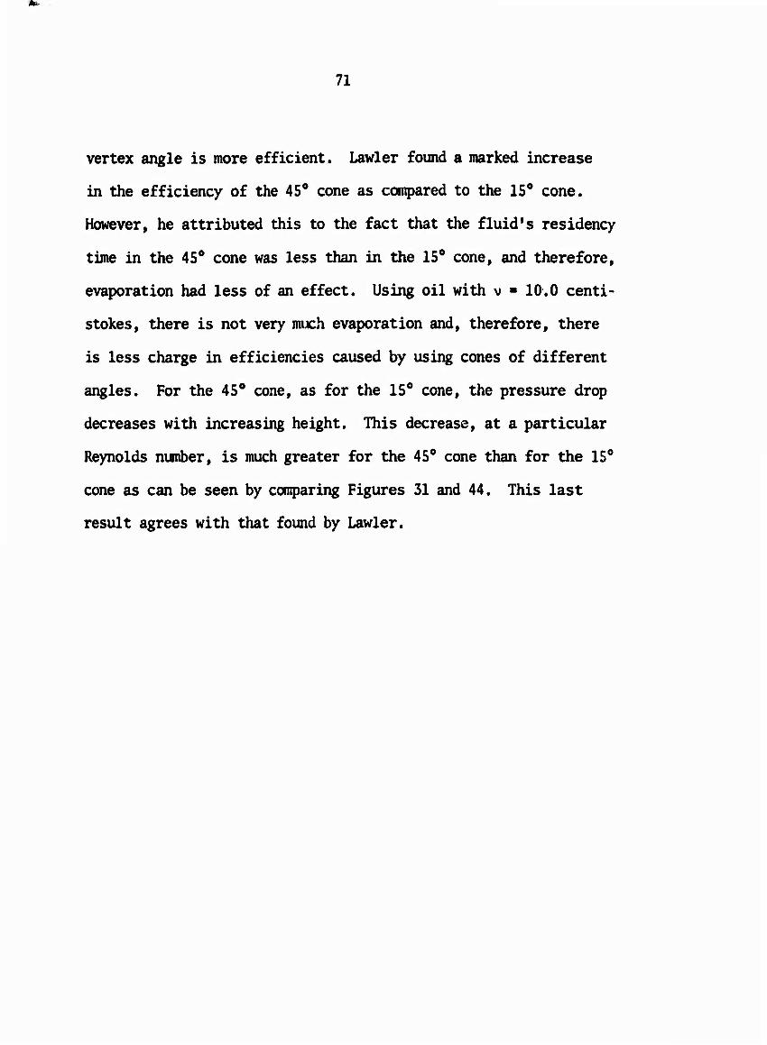
Soultion Of The Boundary Layer Equations By Integral Means

The boundary layer equations for a cone can be written as:

2 2 ,, 3u V . , 3u 1 3p 3 u ,T , . u35r--x + w3l= "Fax* vri (I-la) oZ

2 w32 + u3x + 5r= v-i (I-lb)

3z

-||.0 (I.lc)

£ (ux) ^(wx) - 0 (I.Id)

The reader is referred to Lawler's paper for a detailed derivation

of the above boundary layer equations.

Let v « K(R) where R ■ xsinO

^v = K(x) (1.2)

The inviscid equations give:

p" 3x * x

" p 3x x x (1.3)

86

87

Equations (I.la)- (I.Id) become:

u 3x x w 3Z X v a 2 dZ (I.4a)

3V dV UV 3 V 3z 3X X TIz oZ

(I.4b)

f^ (ux) * ^ (xw) - 0 (I.4c)

The appropriate boundary conditions are:

At2»0: u-V-0 (I.5a)

(1.5b)

Integrating the x-momentum equation, (1.4a), from 0 to d with

respect to z :

5 3u 3U

U 3X W 3Z X X z 3U 3z (1.6)

But: w |H d2 . xxg- iz 3z

u£ dl

88

Also, from equation (1.4a):

3w E u + 3u 3z x 3x

Substituting these into equation (1.6) the integral form of the

x-momentum equation is obtained:

6 "-IV

£ 2 ü-d * x z i K2(x) v2d 3U

dz (1.7)

Integrating equation (1.4b) from 0 to 6 with respect to z and

making use of the boundary conditions one obtains the y-momentum

inegral equation:

-K(x) ^3l^dz + 2 ^d + X z k w dz av

az (1.8)

It is desired that u and v satisfy the boundary conditions,

equations (1.5a) and (1.5b) to meet these conditions let:

u = E(x) K(x) F(n) - E(x) K(x) (n-Zn2 + n3)

v = K(x) ^n) = K(x) (2n-n2)

(I.9a)

(I.9b)

where n = r and E ■ E(x), 6 » 6(x) are unknowns. 6 • ' -

Note that dn • -| - -7 6' dx 6 62

89

•'• üz « 6dn for integration over z at fixed x. (1.9c)

6 » 6 ^f^- «■ dimensionless boundary layer thickness. 1 vL (I.9d)

By substituting the appropriate combinations of equations

(1.9a) and (1,9b) along with equations (1.9c) - (I.9d) into equations

(I. 7) and (I. 8) respectively one obtains:

6i al ^ + T al ^ + -TT- + 2E2{I Iftt Kw 2

496, + -Y^ + 105E = 0 (1.10a)

6i al (E2

) + E2

asr ^i) - %- - *2i -^ln K(X)'120E'0 (I'10b)

By combining these equations and noting that:

2 ar (Es2> •2 4< w 42 + «« E one obtains the final form of the equations:

d. (E2) . . ^ . 5E2 ^ tn K(x) - 51 . 330E2 d-lla) Eö-i

rf 7 i; E6? 7 2 ^ 49E62 |- (E«2) = | -1- + ^ ESj ^ to KCx) ♦ —^ ♦ 285 (I.llb)

xt

90

The initial conditions are: E=61«0atx«1.0 thus, both

equation (l.ila)and (I.Ub) have singularities at their initial

values.

Following Taylor's method (2); Let:

E6^ » A(x-l) and E2= B(x-l)

Substituting these expressions into (1.13a) and (I.Ub) and evaluating

at x = 1.0, it is found that A « 80, B » - 19.1.

Thus £6, « 80(x-l) (I.12a)

E2 » - 19.1(x-l) (I.12b)

Assuming these relations (I.12a)-(i.i2b) to be valid very near

to x « 1.0, it is now possible to obtain new, non-singular initial

conditions.

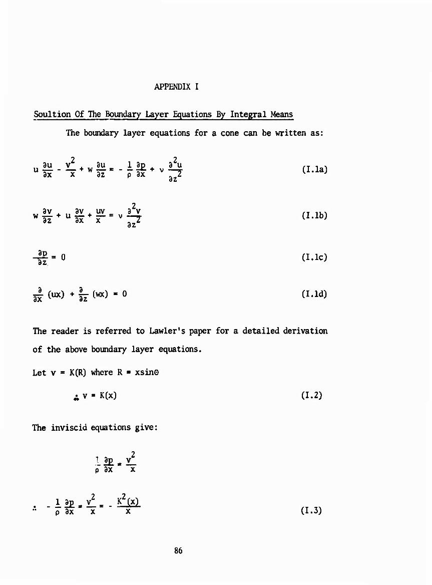
APPENDIX II

Samples of the experimental data are presented on the

following pages. The inlet pressure and the temperature were

measured directly. The heavy fluid outflow rate was determined by

measurements of the volune liquid flow, Q, in a time interval, t.

The pressure drop across the orifice meter, AP, was used to calculate

the volume flow rate of air and, from this, the inlet air velocity.

The inlet oil flow rate was determined from a knowledge of the

nozzle diameter, the pressure drop across the nozzle, PLTQ, and

the oil being sprayed.

91

92

15° Cone

.011 in. Nozzle ; h» 8.25 in. • Lls .0156 ; v = 1.0

P in. in. of F^P in

P . of H20

Temp. oF

PLIQ in. of H

Q ml.

t sec.

1.75 0.30 93.8 26.5 28.5 60.2

5.70 1.00 94.0 26.5 25.5 60.4

10.0 1.80 91.0 26.5 22.8 61.0

13.7 2.40 89.5 26.5 16.5 60.6

18.9 3.20 90.0 26.5 10.0 61.2

2.90 0.50 94.5 26.5 26.5 60.2

5.70 1.00 93.8 26.5 26.0 60.2

10.1 1.80 90.8 26.5 21.5 60.2

13.6 2.40 89.5 26.5 15.5 60.4

18.9 3.20 90.9 26.5 10.0 60.2

13.7 2.40 89.5 26.5 15.5 61.0

0.6 0.10 95.0 50.0 48.2 60.2

1.70 0.30 96.0 50.0 43.5 60.2

2.80 0.50 96.0 50.0 40.0 60.0

5.20 1.00 93.5 50.0 36.8 60.2

9.10 1.80 91.5 50.0 31.0 60.0

11.20 2.40 95.0 50.0 24.5 60.2

15.80 3.20 89.8 50.0 22.8 60.6

0.60 0.10 94.8 50.0 47.5 60.2

93

15° Cone

.011 in. Nozzle ; h - 8.25 in. ; 1^ - .0156 ; v » 1.0

P in. in. of H20

AP in. of H20

Temp. op

PLIQ in. of H

Q ml.

t sec.

1.70 0.30 96.0 50.0 44.2 60.0

2.80 0.50 96.0 50.0 40.5 60.2

5.2 1.00 93.5 50.0 37.5 60.6

9.0 1.80 91.2 50.0 32.8 60.2

11.2 2.40 95.0 50.0 24.5 60.2

8.9 1.80 91.2 50.0 32.8 60.4

11.6 2.40 95.0 50.0 26.0 60.2

15.9 3.20 89.8 50.0 22.2 60.2

.011 in. Nozzle ; h = 4.75 in. I h- ,0174 ; v = 10.0

P in. in. of H20

AP in. of H20

Temp. oF

p rLIQ in. of H

Q ml.

t sec.

0.30 0.05 85.0 17.5 23.4 60.0

0.65 0.10 88.6 17.5 24.0 59.8

1.85 0.30 90.0 17.5 24.0 60.2

3.00 0.50 90.0 17.5 24.0 60.0

5.35 1.00 89.0 17.5 24.0 60.0

0.30 0.05 85.0 17.5 24.0 60.2

0.65 0.10 88.6 17.5 24.0 60.2

94

15° Cone

.011 in. Nozzle ; h = 4.75 in. ; Lj - 0.174 ; v » 10.0

P in. AP in. of H20 in. of H20

Temp. op .P"QH Si.

m. of H

t sec.

1.85 0.30 90.1 17.5 24.0 60.0

3.00 0.50 90.0 17.5 24.5 60.2

5.40 1.00 89.0

15° Cone

17.5 23.8 59.6

.011 in. Nozzle ; h - 8.25 in. ; Lj = .0162 ; v « 10.0

0.30 0.05 88.0 17.5 23.8 60.0

0.60 0.10 89.2 17.5 24.0 60.0

1.80 0.30 92.5 17.5 24.0 61.0

2.80 0.50 92.5 17.5 24.1 60.0

5.70 1.00 92.0 17.5 24.2 60.0

0.30 0.05 88.0 17.5 24.0 59.6

0.65 0.10 89.2 17.5 24.0 60.0

1.80 0.30 92.5 17.5 24.0 59.6

2.80 0.50 92.5 17.5 24.2 60.0

5.65 1.00 92.0

15° Cone

17.5 24.0 60.2

.011 in Nozzle ; h = 8.25 in ; ; 1^ = .0156 ; v = 10.0

0.30 0.05 84.2 17.5 24.8 60.2

0.60 0.10 89.9 17.5 24.2 60.0

95

15° Cone

.011 in Nozzle ; h - 8.25 in. ; ^ - .0156 ; v = 10.0

P in. in. of H20

AP in. of H20

Temp. op

PLIQ in. of H

Q ml.

t sec.

1.80 0.30 91.0 17.5 24.2 60.0

2.80 0.50 91.2 17.5 25.0 60.6

5.70 1.00 89.5 17.5 23.2 60.0

0.30 0.05 86.0 17.5 24.2 60.0

0.60 0.10 90.2 17.5 24.0 60.0

1.75 0.30 91.2 17.5 25.0 60.4

2.80 0.50 91.2 17.5 25.0 60.0

5.65 1.00 89.8

15° Cone

17.5 24.0 60.4

.011 in Nozzle ; h = 8.25 in. ; ^ = .0174 ; v = = 10.0

0.30 0.05 92.0 17.5 24.0 59.8

0.55 0.10 94.0 17.5 23.8 60.2

1.80 0.30 94.8 17.5 23.6 60.2

2.80 0.50 95.0 17.5 23.5 60.0

5.50 1.00 87.0 17.5 23.2 60.2

9.50 1.80 87.5 17.5 24.0 60.0

0.30 0.05 92.0 17.5 24.2 60.4

0.60 0.10 94.1 17.5 24.0 60.2

1.75 0.30 94.8 17.5 23.5 60.0

96

150Cone

0.11 in. Nozzle ; h - 8.25 in. ; ^ - .0174 ; v « 10.0

P in. AP Temp. PLIQ

in. of H

17.5

17.5

17.5

35.0

35.0

35.0

35.0

35.0

35.0

35.0

35.0

35.0

35.0

35.0

35.0

58.4

58.4

58.4

58.4

in. of H20 in. of H20 oF

2.80 0.50 95.0

5.50 1.00 87.0

9.50 1.80 87.5

0.30 0.05 92.5

0.60 0.10 93.0

1.70 0.30 94.0

2.70 0.50 94.5

5.25 1.00 93.5

9.40 1.80 91.0

0.30 0.05 92.5

0.65 0.10 92.0

1.70 0.30 94.0

2.70 0.50 94.5

5.20 1.00 93.5

9.40 1.80 91.0

0.30 0.05 93.2

0.60 0.10 95.0

1.70 0.30 95.8

2.70 0.50 95.4

Q ml.

t sec.

23.8 60.0

23.8 60.0

24.0 60.4

38.4 60.6

38.9 60.0

40.0 60.4

40.0 61.0

39.8 60.2

40.0 60.4

39.0 60.0

39.0 60.4

39.2 60.0

39.0 60.0

40.0 60.6

39.8 60.4

54.5 60.2

54.5 60.0

54.8 60.0

54.2 60.2

07

15° Cone

0.11 in. Nozzle ; h - 8.25 in. ; Lj - .0174 ; v - 10.0

P in. AP in. of H20 in. of H20

Temp. 0F

PLIQ in. of H

Q ml.

t sec.

0.30 0.05 93.2 58.4 53.8 60.0

0.60 0.10 95.0 58.4 54.0 60.0

1.70 0.30 95.8 58.4 54.5 60.4

2.75 0.50 95.2

15° Cone

58.4 54.2 60.4

.011 in. Nozzle ; h- 12.75 in. ' Ll- .0174 ; v - 10.0

0.30 0.05 86.5 17.5 23.5 60.2

0.50 0.10 90.0 17.5 24.5 60.2

1.40 0.30 92.5 17.5 24.0 59.6

2.20 0.50 91.0 17.5 24.0 60.0

4.30 1.00 89.6 17.5 24.0 60.4

0.35 0.05 86.5 17.5 23.5 60.0

0.50 0.10 90.0 17.5 24.0 60.6

1.35 0.30 92.5 17.5 24.0 59.8

2.20 0.50 91.0 17.5 24.0 60.2

4.30 1.00 89.6 17.5 24.0 60.4

15° Cone

.011 in. Nozzle ; h = 15.00 in. ; 1^ « .0174 ; v = 10.0

0.30 0.05 86.9 17.5 23.0 59.6

98

15° Cone

Oil in. Nozzle ; h - 15.00 in. ; L, » .0174 ; v » 10.0

P in. in. of H20

AP in. of H20

Temp 0F

PLIQ in. of H

g

Q ml.

t sec.

0.50 0.10 89.0 17.5 23.8 60.0

1.35 0.30 91.0 17.5 23.6 60.0

2.00 0.50 91.0 17.5 23.5 60.4

4.20 1.00 89.5 17.5] 24.0 60.4

0.30 0.05 86.9 17.5 23.2 60.0

0.50 0.10 89.0 17.5 23.8 60.2

1.30 0.30 91.0 17.5 23.5 60.4

2.00 0.50 91.0 17.5 24.0 60.4

4.20 1.00 89.5] 17.5 24.0 60.6

15° Cone

0.14 in. Nozzle ; h » 8.25 in. ; Lj - .0506 ; v - 100.0

0.60 0.10 98.0 46.0 39.6 60.8

1.50 0.30 98.6 46.0 39.5 60.0

2.40 0.50 95.0 46.0 39.5 60.0

3.70 0.80 95.0 46.0 39.0 57.8

0.60 0.10 98.0 46.0 39.6 60.4

1.50 0.30 98.6 46.0 39.5 60.0

2.50 0.50 95.0 46.0 39.5 60.0

3.70 0.80 95.0 46.0 39.5 60.2

99

15° Cone

.014 in. Nozzle ; h » 12.75 in. ; 1^ » .0506 ; v = 100.0

P in AP Temp. P. Tn Q t in. of H20 in. of H20

0F ^ ^| H ml. sec. g

0.90 0.10 92.0 46.0 38.0 60.0

1.20 0.30 93.0 46.0 38.5 60.4

1.80 0.50 94.0 46.0 38.5 60.2

2.80 0.80 94.2 46.0 38.5 60.4

0.9 0.10 92.2 46.0 38.0 60.0

1.20 0.30 93.0 46.0 39.0 60.2

1.85 0.50 94.0 46.0 38.2 60.4

2.80 0.80 94.2 46.0 38.2 60.2

15° Cone

.014 in. Nozzle ; h « 15.00 in. ; L, » .0506 ; v » 100.0

0.30 0.10 86.2 46.0

1.20 0.30 91.0 46.0

1.70 0.50 91.6 46.0

2.60 0.80 91.2 46.0

0.40 0.10 86.3 46.0

1.15 0.30 91.0 46.0

1.70 0.80 91.2 46.0

2.65 0.80 91.2 46.0

39.0 60.2

39.5 60.4

38.0 60.2

39.5 60.6

39.5 60.2

39.5 60.0

39.5 60.6

39.5 60.4

100

45° Cone

.011 in. Nozzle ; ; h- 8.25 in. ; ; 4-. ,0174 ; v ' « iU.U

P in AP in. of H20 in. of H20

Temp. op

PLIQ in. of H

Q ml.

t sec.

0.60 0.10 93.0 20.0 26.5 60.2

1.70 0.30 94.5 20.0 27.0 60.0

2.25 0.50 94.0 20.0 26.0 60.2

0.60 0.10 93.0 20.0 27.0 60.0

1.65 0.30 94.6 20.0 26.5 60.0

2.20 0.50 94.0

45° Cone

20.0 25.8 59.8

0.11 in Nozzle ; h « ' 8.25 in. ; Ll" .0116 ; v « 10.0

0.40 0.05 89.2 17.5 23.8 60.6

0.70 0.10 91.0 17.5 22.8 60.0

1.80 0.30 92.0 17.5 23.8 60.2

0.40 0.05 89.2 17.5 23.0 60.2

0.70 0.10 91.0 17.5 23.0 60.2

1.75 0.30 92.0

45° Cone

17.5 23.6 61.0

.014 in. Nozzle h « 8.25 in. ; Lls .0182 ; v - 10.0

0.60 0.10 95.6 20.0 26.0 60.2

1.70 0.30 96.6 20.0 26.0 60.0

2.20 0.50 97.0 20-0 25.0 60.2

101

45° Cone

.014 in. Nozzle ; h - 8.25 in. ; Lj - .0182 ; v = 10.0

P in. AP Temp. PITn Q t

in. of H20 in. of H20 0F in. of H m1, sec•

0.55 0.10 95.6 20.0 26.0 60.2

1.70 0.30 96.6 20.0 26.0 60.6

2.20 0.50 97.0 20.0 25.2 60.4

45° Cone

.014 in. Nozzle ; h = 8.25 in. ; 1^ » .0174 ; v = 10.0

0.6 0.10 95.6 50.0

1.5 0.30 96.0 50.0

2.0 0.50 95.0 50.0

0.6 0.10 95.6 50.0

1.6 0.30 96.0 50.0

2.0 0.50 95.0 50.0

45° Cone

.011 in. Nozzle ; h = 12.75 in. ; L, « .0171 ; v « 10.0

0.40 0.10 94.0 20.0

1.35 0.30 94.2 20.0

2.00 0.50 94.5 20.0

0.50 0.10 94.0 20.0

1.40 0.30 94.2 20.0

2.00 0.50 94.4 20.0

49.0 60.6

48.5 60.8

48.5 60.8

49.0 60.4

49.0 61.0

48.0 60.2

27.0 60.0

26.5 60X

25.0 60.2

27.0 60.0

26.0 60.0

25.0 60.4

102

45° Cone

.011 in. Nozzle • h '■ ■- 15.00 in. ; V. ,0175 ; v = 10.0

P in in. of H20

AP in. of H20

Temp. op

PLIQ in. of H

Q ml.

sic.

0.35 0.10 91.0 22.0 25.0 60.4

1.20 0.30 93.8 22.0 24.0 60.4

1.80 0.50 94.0 22.0 22.0 60.2

0.40 0.10 91.0 22.0 24.0 60.2

1.80 0.50 94.0 22.0 23.0 60.2

BIBLOGRAPHY

1. Stromquist, A.J.'/'Zcro Gravity Development For Re-generation Fuel Cell" ASD-TÜR-62-240, (by Thompson Ramo Wooldridge, Inc. For The Flight Accessories Laboratory, ASD, Wright-Patterson AFB, Ohio) 1962.

2. Taylor, G.I.:" The Boundary Layer in The Conveying Nozzle of a Swirl Atomizer',1 Qwart. Jour. Mech. and Appl. Math., Vol. Ill, Pt. 2, pp. 129-139, 1950.

3. ter Linden, A.J.:"Investigations into Cyclone Dust Collectors1,1

Proc. Inst. Mech. Eng. London, Vol. 160, No. 2, pp 233-251, 1949.

4. Van Dongen, J.R.J.; and ter Linden, A.J.^The Application of Gas/Liquid Cyclone in Oil Refining, Trans. ASME, pp. 245-251, Jan., 1958.

5. Moore, F.K.: "Three-Dimensional Boundary Layer Theory", Advances in Applied Mechanics. Vol. IV, pp. 159-228, Academic Press Inc., New York, 1956.

6. Lawler, M.T., "A Study of Cyclonic Two-Fluid Separation, Master's Thesis, Case Institute of Technology, 1965.

103

Security Classification

DOCUMENT CONTROL r%rfir- «ID (Sucurily elmaaiUemtlon ot till», body ol abstract and indexing ennotailCn mual be entered when the overall report te clanailied)

1 OR1GINATIN G ACTIVITY rCoiporafo «urhorj

Case Institute of Technology Fluid, Thermal and Aerospace Sciences Group Cleveland, Ohio

2« REPORT SECURITY C LAISIMCATION

UNCLASSIFIED 2b GROUP

3 REPORT TITLE

LIQUID-GAS CYCLONE SEPARATION

4. DESCRIPTIVE NOTES (Type ot report and Inctualve dalea)

Scientific- Interim, 5. AUTHORfS; (Lmat name, drat name. Initial)

Sanford Fleeter Simon Ostrach

6. REPORT DATE

June 1966 7# TOTAL NO. OF PACES

113 7b NO. OF REFS

8«. CONTRACT OR GRANT NO.

AF-AFOSR 194-66 b. PROJECT NO.

9781-01 e'61445014

*• 681307

9a ORIOINATOR'S REPORT NUMBERfSj

ETAS/TR-66-I2

9b. OTHER REPORT NOfS.) (Any other number» that may be atttgned Ihla report)

AFOSR 66-1400 10- AVAILABILITY/LIMITATION NOTICES

1, Distribution r t-.his document is unlimited.

II. SUPPLEMENTARY NCTUS 12. SPONSORING MILITARY ACTIVITY

AF Office of Scientific Research (SREM) 1400 Wilson Boulevard Arlington, Virginia 22209

13 ABSTRACT

This paper considers the secondary-flow in a liquid-gas mixture in a cyclone separator. By means of a momentum integral method, an engineering approximation to the secondary (heavy fluid) flow rate is obtained which makes use of an experimental velocity profile determined by ter Linden, This flow rate approximation is physically realistic and is partially verified in the laboratory. Tests were run on a separator to determine the effect of the variation of certain operating conditions and geometric factors on the separation of a liquid-gas mixture. The effect of these variations on the efficiency of separation and pressure drop across the separator as functions of the Reynolds and Weber numbers is presented.

DD .^ 1473 Security Classification

■OMHVPsn!

Security Classification u.

KEY WORDS LINK A

ROLE LINK 8

ROLE V»T

LINK C HOLE

Fluid Mixtures Fluid Separation Vortex Flows

INSTRUCTIONS

1. ORIGINATING ACTIVITY: Enter the name and address of the contractor, subcontractor, grantee, Department'of De- fense activity or other organization (corporate author) issuing the report.

2«. REPORT SECURITY CLASSIFICATION: Enter the ovtt- all security classification of the report. Indicate whether "Restricted Data" is included. Marking is to be in accord- ance with appropriate security regulations.

2b. GROUP: Automatic downgrading is specified in DoD Di- rective 5200.10 and Armed Forces Industrial Manual. Enter the group nambe-. Also, when applicable, show that optional markings have been used for Group 3 and Group 4 as author- ized.

3. REPORT TITLE: Enter the complete report title in all capital letters. Titles in all cases should be unclassified. If a meaningful title cannot be selected without classifica- tion, show title classification in all capitals in parenthesis immediately following the title.

4. DESCRIPTIVE NOTES: If appropriate, enter the type of report, e.g., interim, progress, summary, annual, or final. Give the inclusive dates when a specific reporting period is covered.

5. AUTHOR(S): Enter the name(8) of authoKs) as shown on or in the report. Entei last name, first name, middle initial. If military, show rank end branch of service. The name of the principal oinhor is an absolute minimum requirement.

6. REPORT DATH Enter the date of the report us day, month, year; or month, year. If more than one date appears on the report, use date of publication.

7a. TOTAL NUMBER OF PAGES: The total page count should follow normal pagination procedures, i.e., enter the number of pages containing information.

7b. NUMBER OF REFERENCES: Enter the total number of references cited in the report.

8a. CONTRACT OR GRANT NUMBER: If appropriate, enter the applicable numb'.-r of the contract or grant under which the report was written.

8b, 8c, & Sd. PROJECT NUMBER: Enter the appropriate military department identification, such as project number, subproject number, system numbers, task number, etc.

9a. ORIGINATOR'S REPORT NUMBER(S); Enter the offi- cial report number by which the document will be identified and controlled by the originating activity. This number must be unique to this report. Ob. OTHER REPORT NUMBER S): If the report has been assigned any other report numbers (cither by the originator or by the sponsor), also enter this number(s).

10. AVAILABILITV/ LIMITATION NOTICES: Enter any lim- itations on further dissemination of the report, other than those

imposed by security classification, using standard statements such as:

(1)

(2)

(4)

(5)

"Qualified requesters may obtain copies of this report from DDC."

"Foreign announcement and dissemination of this report by DDC is not authorized."

"U. S. Govfc nment agencies may obtain copies of this report directly from DDC. Other qualified DDC users shall request through

"U. S, milito.y agencies may obtain cc-t : s of this report directly from DDC Other qualitied users shall request through

"Ail distribution of this report is controlled. Qual- ified DDC users shall request through

If the report has been furnished to the Office of Technical Services, Department of Cormerce, for sale to the public, indi- cate this fact and enter the price, if known.

11. SUPPLEMENTARY NOTES: Use for additional explana- tory notes.

12. SPONSORING MILITARY ACTIVITY: Enter the name of the departmental project office or laboratory sponsoring .pay- ing for) the research and development. Include address.

13. ABSTRACT: Enter an abstract giving a brief and factual summary of the document indicative of the report, even though it may also appear elsewhere in the body of the technical re- port. If additional space is required, a continuation sheet shall be attached.

It is highly desirable that the abstract of classified reports be unclassified. Each paragraph of the abstract shall end with an indication of the military security classification of the in- formation in the paragraph, represented as (TS). (S). (C). or (U).

There is no limitation en the length of the abstract. How- ever, the suggested length is from 150 to 225 words.

14. KEY WORDS: Key words are technically meaningful terms or short phrases that characterize a report and may be used as index entries for cataloging the report. Key words must be selected so that no security classification is required. Identi- fiers, such as equipment mode, designation, trade name, military project code name, geographic location, may be used as key words bat will be followed by an indication of technical con- text. The assignment of links, rules, and weights is optional.

GPO B86-551

i(,'curit\ Classific ition