Embed Size (px)
Citation preview

INSTABILITIES, NUCLEATION, AND CRITICAL BEHAVIOR
IN NONEQUILIBRIUM DRIVEN FLUIDS
THEORY AND SIMULATION


Institute ‘Carlos I’ for Theoretical and Computational Physics
and Depto. de Electromagnetismo y Fısica de la Materia
Universidad de Granada, Spain
INSTABILITIES, NUCLEATION, AND CRITICAL BEHAVIOR
IN NONEQUILIBRIUM DRIVEN FLUIDS
THEORY AND SIMULATION
MANUEL DIEZ MINGUITO
email: [email protected]: http://cahn.ugr.es/∼mdiez
Advisor: Prof. Dr. Joaquın Marro
Ph.D. Thesis
Granada, September 2006

To Linda

[...] debemos nosotros tener correctamenteuna explicacion sobre los fenomenos celestes,
que principio determina las trayectorias del sol y la lunay que fuerza rige a cada cosa en la tierra.
Lucrecio. De rerum natura.

Acknowledgments
Esta etapa de mi vida se cierra con dos nacimientos: en marzo, mi hija Cora yahora, esta tesis. Mientras que las sensaciones que me produce el primero quedanen familia, debo expresar aquı mi agradecimiento a quienes han contribuido alsegundo.
En primer lugar quiero agradecer a Joaquın Marro, mi profesor, tutor y men-tor, todo el apoyo incondicional que me ofrecio desde el principio, sabiendo siem-pre que era lo mejor para mı en cada momento. A Pedro Garrido le agradezcotodo el tiempo dedicado, su modo tan especial de motivar, las muchas dudasresueltas y las planteadas tambien, y su franqueza. Parte de este trabajo se ladebo a la intuicion de Paco de los Santos, mi companero de despacho con el quehe compartido muy buenos ratos y charlas sinceras y de cuyo humor inteligentehe disfrutado. Asimismo agradezco a Miguel Angel Munoz, para mı un modeloa seguir, su interes, apoyo y consejo en momentos muy oportunos. Y al restode los componentes del grupo de Fısica Estadıstica: Omar, mi companero deviaje durante estos ultimos cuatro anos, siempre cordial, altruista y dispuesto,David Navidad, Jesus Cortes, Pablo Hurtado, Abdelfattah Achahbar, AntonioL. Lacomba, Joaquın Torres, Don Jesus Biel y Paco Ramos. Sin el ambiente detrabajo y camaraderıa presente en el grupo, sencillamente esta tesis no hubierallegado a buen puerto.
Siento una especial gratitud tanto a nivel profesional como personal haciaBaruch Meerson. Aun me sorprenden su compromiso y dedicacion, sus sincerosconsejos, ası como su carino y cercanıa, los cuales me ayudaron a creer enesta tesis y estan mas alla de todo elogio. Tampoco podre olvidar el excelenterecibimiento que me brindaron el y su esposa en esa ciudad maravillosa que esJerusalen.
Durante estos anos he tenido dos buenos colaboradores en Thorsten Poschely Thomas Schwager, a los que les agradezco su interes y la doblemente buenaacogida dispensada en Berlın.
Que importantes han sido los amigos, siempre presentes, de los que hay pocoque decir y mucho que agradecer. En este periplo he tenido la gran suerte deconocer a Juan Antonio, igualmente miembro del grupo. Con el he compartidoinnumerables charlas, preocupaciones, confidencias, confianza, amistad. Gra-cias. A mis ya viejos amigos: Fernando, que tambien sabe lo que es hacer unatesis luchando dıa a dıa a tocapenoles, le debo su experiencia y su apoyo en mo-mentos difıciles; a Miguel, para mı mas que un amigo, por la ilusion y el tiempo

x Acknowledgments
que juntos invertimos en tantos proyectos; a Jesus, por su ejemplar honradez yfidelidad, y al resto de los miembros del equipo.
A mis padres, que lo han dado todo por mı. A Gabi, Holger y Christoph,por su continuo interes y carino.
A Cora, porque a pesar de haber demorado la redaccion de este trabajo meha alegrado la vida. Y finalmente a Linda, mi esposa y mi guıa, a quien lededico esta tesis. Gracias por todo, lo decible y lo indecible.
Granada, a 17 de Septiembre de 2006.

Contents
Acknowledgments ix
1 General Introduction 1
1.1 Overview . . . . . . . . . . . . . . . . . . . . . . . . . . . . . . . 7
Part I Driven Diffusive Fluids 11
2 Introduction 13
3 Lennard–Jones and Lattice models of driven fluids 19
3.1 Driven Lattice Gas . . . . . . . . . . . . . . . . . . . . . . . . . . 19
3.2 Driven Lennard-Jones fluid . . . . . . . . . . . . . . . . . . . . . 22
3.3 Driven Lattice Gas with extended dynamics . . . . . . . . . . . . 24
3.3.1 Correlations and Structure Factor . . . . . . . . . . . . . 24
3.3.2 Critical behavior . . . . . . . . . . . . . . . . . . . . . . . 27
3.4 Conclusions . . . . . . . . . . . . . . . . . . . . . . . . . . . . . . 33
4 Anisotropic phenomena in nonequilibrium fluids 35
4.1 Motivation . . . . . . . . . . . . . . . . . . . . . . . . . . . . . . 35
4.2 The model . . . . . . . . . . . . . . . . . . . . . . . . . . . . . . . 37
4.3 Main results . . . . . . . . . . . . . . . . . . . . . . . . . . . . . . 39
4.3.1 Phase segregation kinetics . . . . . . . . . . . . . . . . . . 39
4.3.2 Structure of the steady state . . . . . . . . . . . . . . . . 43
4.3.3 Transport properties . . . . . . . . . . . . . . . . . . . . . 45
4.3.4 Coexistence curve . . . . . . . . . . . . . . . . . . . . . . 46
4.4 Conclusions . . . . . . . . . . . . . . . . . . . . . . . . . . . . . . 49
Part II Driven Granular Gases 53
5 Introduction 55
xii CONTENTS
6 Phase separation of a driven granular gas in annular geometry 61
6.1 Introduction . . . . . . . . . . . . . . . . . . . . . . . . . . . . . . 626.2 Particles in an annulus and granular hydrostatics . . . . . . . . . 63
6.2.1 The density equation . . . . . . . . . . . . . . . . . . . . . 636.2.2 Annular state . . . . . . . . . . . . . . . . . . . . . . . . . 656.2.3 Phase separation . . . . . . . . . . . . . . . . . . . . . . . 67
6.3 Molecular Dynamics Simulations . . . . . . . . . . . . . . . . . . 706.3.1 Method . . . . . . . . . . . . . . . . . . . . . . . . . . . . 706.3.2 Steady States . . . . . . . . . . . . . . . . . . . . . . . . . 716.3.3 Azimuthal Density Spectrum . . . . . . . . . . . . . . . . 73
6.4 Conclusions . . . . . . . . . . . . . . . . . . . . . . . . . . . . . . 76
7 Close–packed granular clusters 79
7.1 Introduction . . . . . . . . . . . . . . . . . . . . . . . . . . . . . . 797.2 Event–driven molecular dynamics simulations . . . . . . . . . . . 807.3 Hydrostatic theory . . . . . . . . . . . . . . . . . . . . . . . . . . 827.4 Macro–particle fluctuations . . . . . . . . . . . . . . . . . . . . . 887.5 Conclusions . . . . . . . . . . . . . . . . . . . . . . . . . . . . . . 89
Part III Appendices 93
A Equilibrium properties of the Lattice Gas 95
B Interfacial stability of Driven Lattice Gases for E → ∞ 99
C Mesoscopic equation for the DLG with extended dynamics 105
D Hydrodynamics for three-dimensional granular gases 109
Part IV Conclusions 115
Conclusions and future work 117
Published work 125
Bibliography 127
Resumen en Espanol 139
List of Figures
1.1 Complexity of the macroscopic behavior . . . . . . . . . . . . . . 3
2.1 Typical configurations in the stationary regime of the DLG for a128 × 128 half-filled lattice . . . . . . . . . . . . . . . . . . . . . . 14
3.1 Typical steady state configurations of the DLJF subject to a hor-izontal field . . . . . . . . . . . . . . . . . . . . . . . . . . . . . . 21
3.2 Schematic phase diagrams for the DLG, NDLG, and DLJF . . . 233.3 Triangular anisotropies observed at early times of the DLG and
DLJF . . . . . . . . . . . . . . . . . . . . . . . . . . . . . . . . . 24
3.4 Schematic comparison of the sites a particle may occupy fornearest–neighbor and next–nearest–neighbor hops . . . . . . . . . 25
3.5 Surface plots of the two–point correlations and structure factorabove criticality for the DLG with NN and NNN couplings . . . 25
3.6 Parallel and transverse components of the two-point correlationfunction above criticality for the DLG with NN and NNN inter-actions . . . . . . . . . . . . . . . . . . . . . . . . . . . . . . . . . 26
3.7 Parallel and transverse components of the structure factor abovecriticality for the DLG with NN and NNN interactions . . . . . . 27
3.8 Log-log plot of the rescaled order parameter m for different sizes 29
3.9 Log-log plot of the rescaled susceptibility χ for different sizes . . 293.10 Scaling plot of the rescaled fourth Binder cumulant b for different
sizes . . . . . . . . . . . . . . . . . . . . . . . . . . . . . . . . . . 30
4.1 Off–lattice models in the realm of computer simulation of fluids . 36
4.2 Schematic representation of the region which is accessible to agiven particle as a consequence of a trial move . . . . . . . . . . 38
4.3 Typical steady–state configurations for equilibrium (E = 0) andlarge field limit (E → ∞) . . . . . . . . . . . . . . . . . . . . . . . 40
4.4 Typical configurations for E = 0 and E → ∞ as time proceedsduring relaxation from a disordered state . . . . . . . . . . . . . 41
4.5 Time evolution of the enthalpy or excess of energy per particlefor different temperatures . . . . . . . . . . . . . . . . . . . . . . 42
4.6 Details of the structure in the low−T, solid phase . . . . . . . . . 43
xiv LIST OF FIGURES
4.7 Degree of anisotropy (main graph), radial (lower inset) and az-imuthal (upper inset) distribution functions . . . . . . . . . . . . 44
4.8 Transverse–to–the–field current profiles below criticality: com-parison between lattice and off-lattice models . . . . . . . . . . . 46
4.9 Temperature dependence of the mean energy and normalized netcurrent for large field limit . . . . . . . . . . . . . . . . . . . . . . 47
4.10 Density profiles transverse to the field for different temperatures 474.11 Liquid–vapor coexistence curve and the associated critical in-
dexes obtained from the density profiles . . . . . . . . . . . . . . 49
6.1 The normalized density profiles obtained from simulations andhydrostatics . . . . . . . . . . . . . . . . . . . . . . . . . . . . . . 66
6.2 Main Graph: The marginal stability curves k = k(f) at fixedaspect ratios Ω for different values of the heat loss parameter Λ.Inset: The dependence of kmax on Λ1/2 . . . . . . . . . . . . . . 67
6.3 Two-dimensional projections of the phase diagram: Marginal sta-bility and negative compressibility curves . . . . . . . . . . . . . 68
6.4 The scaled steady state granular pressure P versus the grain areafraction f at fixed Ω, and the spinodal interval . . . . . . . . . . 70
6.5 Typical steady state snapshots . . . . . . . . . . . . . . . . . . . 716.6 Typical steady state snapshots and the temporal evolution of the
COM and of the squared amplitude of the fundamental Fouriermode . . . . . . . . . . . . . . . . . . . . . . . . . . . . . . . . . . 72
6.7 The normalized probability distribution functions at a differentnumber of particles . . . . . . . . . . . . . . . . . . . . . . . . . . 74
6.8 The Ω-f phase diagram for Λ = 81.09 obtained from moleculardynamics simulations and hydrodynamics . . . . . . . . . . . . . 76
6.9 The marginal stability lines for our main setting and for an al-ternative setting . . . . . . . . . . . . . . . . . . . . . . . . . . . 77
7.1 Snapshots and magnifications of the close–packed cluster . . . . . 817.2 Scaled density n/nc: Comparison between hydrostatics and event–
driven simulations . . . . . . . . . . . . . . . . . . . . . . . . . . 847.3 Maximum scaled density nmax/nc: Comparison between hydro-
statics and event–driven simulations . . . . . . . . . . . . . . . . 867.4 Marginal stability curve (main graph) and eigenfunctions associ-
ated to the linear eigenvalue problem (inset) . . . . . . . . . . . . 877.5 Probability distribution functions of the center of mass of the
macro–particle . . . . . . . . . . . . . . . . . . . . . . . . . . . . 887.6 Scaled standard deviation of the center of mass position . . . . . 90
A.1 Spontaneous magnetization and order parameter critical expo-nent for the Ising model with NN and NNN couplings . . . . . . 96
A.2 Surface plots of the two–point correlations and structure factorabove criticality for the equilibrium lattice gas with NN and NNNinteractions . . . . . . . . . . . . . . . . . . . . . . . . . . . . . . 97

LIST OF FIGURES xv
A.3 Projections of the two–point correlations and structure factorabove criticality for the equilibrium lattice gas . . . . . . . . . . 98
B.1 Schematic diagram of the accessible sites for a particle in theαDLG model . . . . . . . . . . . . . . . . . . . . . . . . . . . . . 101
B.2 The α-dependence of the order parameter m in the αDLG . . . . 102B.3 Order parameter critical exponent for the second order phase
transition which occurs in the αDLG . . . . . . . . . . . . . . . . 103
D.1 Perspective sketch of the three-dimensional experimental set-up . 110D.2 Scaled temperature and density profiles as predicted by granular
hydrostatic theory in three dimensions . . . . . . . . . . . . . . . 112D.3 Marginal stability curve m = m(f) (main graph) and eigenfunc-
tions Γm(r) (inset) . . . . . . . . . . . . . . . . . . . . . . . . . . 113
D.4 Complejidad del comportamiento macroscopico . . . . . . . . . . 141
xvi LIST OF FIGURES
List of Tables
4.1 Critical parameters . . . . . . . . . . . . . . . . . . . . . . . . . . 48
6.1 The averaged squared relative amplitudes 〈A2k(t)〉/a2
0 for the firstthree modes k = 1, 2 and 3 . . . . . . . . . . . . . . . . . . . . . . 75
xviii LIST OF TABLES
Chapter 1
General Introduction
Nature has a hierarchical structure, with time, length, and energy scales rang-ing from the microscopic to the macroscopic. Surprisingly, it is often possibleto discuss these levels independently, e.g., in the case of molecular fluids. Themacroscopic level, i.e. the world directly perceived at our human senses, isdescribed hydrodynamically. That is, by continuous (or piecewise continuous)functions of the spatial coordinates r and time t (hydrodynamic fields). Asa result, the great disciplines of macroscopic physics, such as fluid mechanics,elasticity, acoustics, electromagnetism, are field theories. These fields are deter-mined by integro-differential equations involving unknown functions of r andt. The microscopic level is described as a collection of a very large number ofconstituents, such as atoms, molecules, or other more complex entities inter-acting with each other through well-defined electro-mechanical forces1. Theirevolution with time is provided by the laws of quantum mechanics, but in manycases classical mechanics results a good approximation.
If there is a clear scale separation between microscopic and macroscopic,then an intermediate scale can be introduced. Such a level of description isreferred to as the mesoscopic level. It is a coarse–grained representation to cap-ture the physics of microscopic models on the large length and time scales, whichis described by stochastic partial differential equations [1, 2]. By concreteness,the mesoscopic description of the system in question, whose dynamics is on theaverage governed by the laws of macroscopic time evolution, is a result of build-ing up of microscopic fluctuations. This approach aims at understanding theslowly-varying long wavelength, low frequency properties of many-body systemsand form the basis of the field theoretical analyses of critical phenomena. In theliterature it is common include in this intermediate scale the kinetic descriptionof gases, e.g., Boltzmann equation. Thus, this level is also referred to as the
1The difference between microscopic and macroscopic levels is essentially relative. The keyconcept here is the large number of constituents, not their small size. For instance, a galaxy(macroscopics) is a object composed by a large number of stars (microscopics), a colony oforganisms is a large set of individuals, a gas comprised by a large number of molecules, etc.
2 General Introduction
kinetic level2. This is in fact a reduced microscopic level, described by one-particle coarse-grained distribution functions and the asymptotic, irreversiblekinetic equations.
The three different levels of description3 are, in principle, equivalent ap-proaches of the same reality. Nevertheless, the form of the laws derived at thesethree levels are so different from each other that there soon appeared a stringentneed for an explanation of hydrodynamics in terms of the microscopic evolu-tion of the underlying collection of constituents. The bridges between them areprovided by Statistical Mechanics. Statistical mechanics aims to derive macro-scopic behavior of matter originated in the cooperative behavior of interacting(microscopic) individual entities. Some of the phenomena are simple synergeticeffects of the actions of individuals, e.g., the pressure exerted by a moleculargas on the walls of its container and thousands of fireflies flashing in synchrony;while others are paradigms of emergent behavior, having no direct counterpartin the properties or dynamics of individual constituents, e.g., the transition fromlaminar to turbulent flows in fluids and the one million of atoms which give riseto the program of life: the deoxyribonucleic acid or DNA for short. In the lattercases, the behavior of the constituents become singular, but very different fromwhat they would exhibit in the absence of the others.
The most successful achievement of statistical mechanics is Ensemble Theory[3], which yields the connection between the macroscopic properties of equilib-rium systems from the laws governing the microscopic interactions of the in-dividual particles. It is said that a certain system stay at equilibrium whenit is isolated, shows no hysteresis, and reaches a steady state (all its macro-scopic properties are fixed) [4]. In that case, the macroscopic properties areexpressed in terms of thermodynamic variables. Indeed, the thermodynamics isin this sense a kind of hydrodynamic description, which consists only of laws andrelations between thermodynamic quantities. From the mathematical point ofview, ensemble theory can be completely axiomatized. This provides us, at leastin principle, analytic expressions for these thermodynamic quantities allowingus to derive all the relevant macroscopic information of the thermal system inquestion4, e.g., the free energy, equation of state, etc.
In nature, by contrast, equilibrium systems are an exception (even an ideal-ization) rather than the rule: non-equilibrium phenomena are overwhelminglymore abundant. Galaxies, human beings, chemical reactions, geophysical flows,carriers in semiconductor devices, financial stock markets, ratchet-effect trans-port, traffic flow on a highway, to cite just a few, are (many-body) systems
2Formally, both stochastic differential equations and kinetic equations may belong to thesame level, although they involve different (mesoscopic) length and time scales.
3There may be larger scale structures (e.g., the Karman vortex train) produced by a largescale fluid dynamics, but we do not pay attention to such large scales.
4Once the microscopic Hamiltonian (say H) of the system is specified the “canonical” sta-tionary probability distribution P is known in terms of the Boltzmann factor P = e−H/kBT /Z,where Z is the partition function, kB is the Boltzmann’s constant, and T the temperature.Thus, averages over such a distribution of time-independent observables can be computed.The remaining difficulties are merely technical.
3
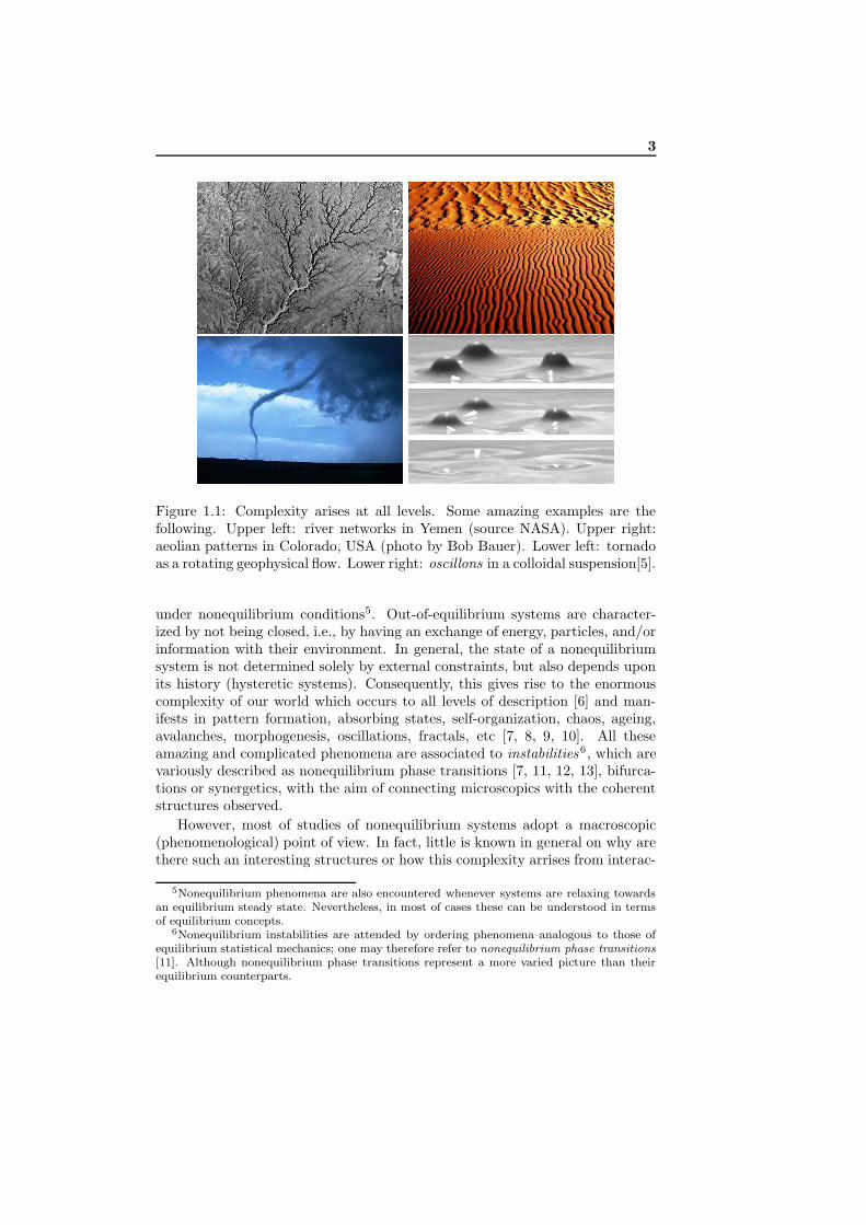
Figure 1.1: Complexity arises at all levels. Some amazing examples are thefollowing. Upper left: river networks in Yemen (source NASA). Upper right:aeolian patterns in Colorado, USA (photo by Bob Bauer). Lower left: tornadoas a rotating geophysical flow. Lower right: oscillons in a colloidal suspension[5].
under nonequilibrium conditions5. Out-of-equilibrium systems are character-ized by not being closed, i.e., by having an exchange of energy, particles, and/orinformation with their environment. In general, the state of a nonequilibriumsystem is not determined solely by external constraints, but also depends uponits history (hysteretic systems). Consequently, this gives rise to the enormouscomplexity of our world which occurs to all levels of description [6] and man-ifests in pattern formation, absorbing states, self-organization, chaos, ageing,avalanches, morphogenesis, oscillations, fractals, etc [7, 8, 9, 10]. All theseamazing and complicated phenomena are associated to instabilities6, which arevariously described as nonequilibrium phase transitions [7, 11, 12, 13], bifurca-tions or synergetics, with the aim of connecting microscopics with the coherentstructures observed.
However, most of studies of nonequilibrium systems adopt a macroscopic(phenomenological) point of view. In fact, little is known in general on why arethere such an interesting structures or how this complexity arrises from interac-
5Nonequilibrium phenomena are also encountered whenever systems are relaxing towardsan equilibrium steady state. Nevertheless, in most of cases these can be understood in termsof equilibrium concepts.
6Nonequilibrium instabilities are attended by ordering phenomena analogous to those ofequilibrium statistical mechanics; one may therefore refer to nonequilibrium phase transitions
[11]. Although nonequilibrium phase transitions represent a more varied picture than theirequilibrium counterparts.
4 General Introduction
tion at a microscopic level. Consequently, no theory exists and the developmentof a solid theoretical background is nowadays in an early stage compared withequilibrium, where the ensemble theory holds successfully. As a matter of fact,the key point of difference between equilibrium and nonequilibrium statisticalmechanics is that whereas in the former case the stationary probability distribu-tion is known, out of equilibrium one must find the time-dependent distribution,which obey a general evolution equation, i.e., a master equation. In most of sol-uble cases —which in fact are just a few—, this can be done only approximately.One can only provide some unified view when the systems are not too far 7 fromequilibrium [14], where the system can be treated perturbatively around theequilibrium state and studied using linear response theory. Nevertheless, ourattention here lies at systems far from equilibrium where such schemes breakdown.
Within the framework given above, the main subject of this thesis
rests on the study —at different levels of description— of instabilities
in systems which are driven, i.e., maintained far from equilibrium
by an external forcing. We focus here on two main classes, namely,
driven–diffusive fluids and driven granular gases.
The first family (driven–diffusive fluids8) corresponds to systems which are9
coupled to two reservoirs of energy in such a way that there is a steady energyflow through the system. Clearly, this definition comprises a bunch of very var-ied systems. We restrict ourselves to systems in which a (non-zero) current ofparticles (whose number is a conserved quantity) is set up through the system,there is spatial anisotropies associated with an external driving field, and even-tually a nonequilibrium steady state is reached. The simplest example seems tobe a resistor gaining energy from a battery and losing it to the atmosphere. Buteven for this reduced class of systems the stationary probability distribution isunknown.
The basic motivation behind the introduction of driven–diffusive fluids cor-responds to a need of unravel the key ingredients of nonequilibrium behavior.A reasonable approach consist in investigating systems as simple as possible,which aim for capture the microscopic essentials yielding to the complicate,macroscopic nonequilibrium ordering. These microscopic models are usuallyoversimplified representations of real systems, and consider entities as particlesinteracting via simple rules. Between them, lattice models —which are based indiscretization of space into lattice sites— have played a important role due tothe fact that they sometimes allow for exact results, and allow one to isolate the
7Nevertheless, a precise definition of not too far is rather difficult to give; the borderlineis rather unclear.
8We should mention here that in the literature these systems are commonly referred asdriven–diffusive systems instead of driven–diffusive fluids, which is adopted in this thesis.As we shall describe in some detail in Chapter 3, we reserve the former denomination for amean–field mesoscopic description.
9Following Schmittmann & Zia in Ref. [15].

5
specific features of a system. In addition, lattice models allow us to obtain theintuition one needs in order to develop the appropriate theoretical tools and,from a experimental point of view, are easier to be implemented in a computer.Such an approach has given rise to a lively research activity in the last decade[11, 15, 16, 17, 18, 19, 20] and a bunch of emerging techniques may now beapplied to lattice systems, including nonequilibrium statistical field theory. Ageneral amazing result from these studies is that lattice models often capturesome essentials of social organisms [21, 22, 23], formation of river networks [24],epidemics [25], glasses, electrical circuits, traffic [26, 27], hydrodynamics, col-loids and foams, enzyme biology [28], living organisms [29], and markets [30],for example. In particular, lattice models have succeed in understanding (equi-librium) phase transitions and critical phenomena [16, 31, 32] due, in manyaspects, to renormalization group methods [33, 34].
The central result in (equilibrium) critical phenomena is universality, i.e.,the behavior of disparate systems in the vicinity of critical points are deter-mined solely by basic features —dimensionality, range of forces, symmetries,etc.— and does not seem to depend to any great extent on the particular sys-tem [33, 35, 36]. One can therefore hope to assign all systems to classes eachof them being identified by a set of critical indices (exponents and some am-plitude ratios). How much of these concepts apply to nonequilibrium phasetransitions are only just emerging, and one expects lattice models to be equallyimportant here. These issues are considered in Chapter 3, in which a particulardriven-diffusive lattice model, prototype for nonequilibrium phase transitions,is investigated. However, a well-known disadvantage of lattice models is thatwhen they are compared directly with experiment result too crude. This hasto be understood in the sense that they often do not account for importantfeatures of the corresponding nonequilibrium phase diagram, such as structural,morphological, and even critical properties. Furthermore, theoreticians oftentend to consider them as prototypical models for certain behavior, a fact whichis in many cases not justified. This will be discussed in Chapter 4, where weintroduce a novel, realistic model for computer simulation of anisotropic fluids.
The second class of systems we consider in this thesis concerns driven granu-lar gases. A granular material is a large conglomerate of discrete macroscopic10
(classical) particles. Examples, which occur at very different length scales, mayrange from powders to intergalactic dust clouds; they include sand, concrete,rice, volcanic flows, Saturn ring’s, and many others (for a review, see [37]). Theyhave important applications in industrial sectors as pharmaceutical, construc-tion and civil engineering, chemical, food and agricultural, etc. On a largerscale, they are also relevant in understanding many geological and astrophysicalprocesses. In addition, they are closely related to a broader class of systems,such as foams, colloids and glasses. The collective behavior of an assembly ofgranular particles exhibits an impressive variety of phenomena11 which include
10In the sense that they are directly perceived at our human eyes.11The size range of phenomena goes from ≈ 10−6m in powders, to ≈ 103m in deserts, up
6 General Introduction
a plethora of pattern forming instabilities [38, 39, 40, 41], clustering [42, 43, 44],flows and jamming in hoppers [45], avalanches and slides [46], mixing and seg-regation [47], convection and heaping [48, 49], eruptions [50, 51], to cite justa few. Clearly, their relevancy is beyond any doubt, and understanding theirproperties is not only an urgent industrial need, but also an important challengefor physicists.
Since grains have a macroscopic size, friction and restitutional losses fromcollisions give rise to dissipative interactions —kinetic energy is continuallytransferred into heat—. Although the dominant interactions depend on particlesize. The relevant energy scale for a typical, say, rice grain of length l ≈ 5mm
and mass m is its potential energy mgl, where g is the gravitational accel-eration. For much smaller grain sizes other kind of interactions may becomeimportant12. Hence, in granular materials the thermal energy kBT is irrele-vant, i.e. kBT mgl. This implies that dynamical effects outweigh entropyconsiderations [37] and, therefore, neither equilibrium statistical–mechanics northermodynamics arguments are useful. Furthermore, due to the fact that gran-ulates are comprised by a finitenumber of particles13usually there is a strongeffect of fluctuations and, therefore, statistics may be dominated by rare events.Other important effects involve the interstitial fluid, e.g. air or water, althoughin many situations one can ignore it with confidence and consider the grain–grain interactions alone. In this thesis (specifically in Part II) we will restrictourselves to dry granular systems, where the interaction between particles takeplace mainly via contact forces.
However, in spite of the simple (classical) features which characterize them,granular materials behave in a rather unconventional way: their phases —solid,liquid, and gas— have complex–collective properties that distinguish them frommolecular fluids and solids. As a result, their statistics and dynamics are poorlyunderstood. In fact, from a theoretical point of view, these systems are stillonly understood in terms of predictions of a general nature and many openquestions remain. Linear elasticity does not apply for granular solids, which arehighly histeretic, show static stress indeterminacy, and possess static yield shearstress. The interlocking of grains leads to force chains, jamming, dilation onshearing, etc. Liquids are viscous, show avalanches (possess a critical slope), sizesegregation in mixtures, shear bands (narrow regions separating blocks movingwith different velocities), pattern formation. Gases, which can only persistwith continuous energy supply, are highly compressible, show clustering, longrange correlations, inelastic collapse in computational models, non-maxwelliandistribution functions, pattern formation, and lack of scale separation betweenmacroscopic scales and microscopic ones. All of this phenomenology makesdifficult to cast them in the framework of the classical three different phases of
to ≈ 1020m in planetary rings.12For instance, it may occur charging and surface coating for d ≈ 0.1, or magnetization and
surface adhesion for d ≈ 0.01.13In contrast with molecular systems N << NA, where NA is the Avogadro number.
Nevertheless, in certain cases a few thousands or even hundreds of particles are enough toallow for statistical approaches.
1.1 Overview 7
matter. Some of the interesting open issues and controversies that we address inChapters 6 and 7 are: What are the statistical properties of granular systems,how do granular phase changes occur, and what are the optimum continuummodels and when do they apply. In particular, we focus on the continuumdescription of clustering, symmetry breaking, and phase separation instabilitiesin granular gases. As we shall see, these instabilities provide sensitive teststo models of granular flows and contribute to the understanding of patternformation far from equilibrium.
1.1 Overview
We investigate in this thesis the two aforementioned classes of systems, whichhave become of paramount importance in the last years. The study is dividedinto four parts. The Part I, which comprises Chapters 2, 3 and 4, is devoted todriven-diffusive fluids. Part II deals with driven granular gases, and consists ofChapters 5, 6 and 7. Part III includes the Appendix A, B, C, and D. Finally,we close (Part IV) with a detailed summary and the main conclusions.
The first part begin in Chapter 2 by introducing the driven lattice gas —prototype for nonequilibrium anisotropic phase transitions—. This model maybe viewed as an oversimplification of certain traffic and flow problems. The par-ticles interact via a local anisotropic rule, which induces a preferential hoppingalong one direction, so that a net current sets in if allowed by boundary condi-tions. We discuss some of its already known properties and controversies. Weshall describe in greater detail the computational and field–theoretical methodsemployed in Chapters 3 and 4.
One of the most important questions we can ask about any model is whetherthe behavior that it displays is universal. In Chapter 3 we address this questionand study the phase segregation process in the prototypical lattice (microscopic)model introduced in Chapter 2. The emphasis in our study is on the influenceof dynamic details on the resulting (non-equilibrium) steady state, although wealso pay some attention to kinetic aspects. In particular, we shall discuss onthe similarities and differences between the driven lattice gas and related latticeand off–lattice models, from a simulational and theoretical point of view. Thecomparison between them allows us to discuss some exceptional, hardly realisticfeatures of the original driven lattice gas. In addition, we test the validity ofthe two competing mesoscopic (Langevin–type) approaches on describing thecritical behavior of these models.
We introduce in Chapter 4 a novel, realistic off–lattice driven fluid foranisotropic behavior. We describe short–time kinetic and steady–state prop-erties of the non–equilibrium phases, namely, solid, liquid and gas anisotropicphases. This is a computationally–convenient model which exhibits a net cur-rent and striped structures at low temperature, thus resembling many situations

8 General Introduction
in nature. We here focus on both critical behavior and some details of the nu-cleation process. Concerning the critical behavior, we discuss on the role ofsymmetries on computer and field–theoretical modeling of non-equilibrium flu-ids. In addition, some important comparisons with experiments are drawn.
Chapter 5 serves as an introduction to Part II, which is devoted to drivengranular gases. We briefly outline the current situation with regard to researchon granular gases. In particular, we discuss on the applicability of a hydrody-namic theory to granular flows. We also present the basic ingredients of thestudied models and the computer simulation methods.
In Chapter 6 we address phase separation instability of a monodispersegas of inelastically colliding hard disks confined in a two-dimensional annulus,the inner circle of which represents a “thermal wall”. Our main objectives areto characterize the instability and compute the phase diagram by using granu-lar hydrodynamics —we employed for hydrodynamics Enskog–type constitutiverelations, which are derived from first principles— and event driven moleculardynamics simulations. We also discuss on clustering and symmetry-breakinginstabilities. By focusing on the annular geometry, we hope to motivate experi-mental studies of the granular phase separation which may be advantageous inthis geometry.
This Chapter 7 addresses granular hydrodynamics and fluctuations in asimple two–dimensional granular system under conditions when existing hydro-dynamic descriptions break down because of large density, not large inelasticity.We study a model system of inelastically colliding hard disks inside a circularbox, driven by a thermal wall in which a dense granular cluster behave like amacro-particle. Some features of the macro–particle are well described by thestationary solution of granular hydrostatic equations by using phenomenologi-cal constitutive relations. Hydrostatic predictions are tested by comparing withmolecular dynamics simulations. We are able to develop an effective Langevindescription for the macro-particle, confined by a harmonic potential and drivenby a delta-correlated noise. We are also concerned about whether the crystalstructure depends on the geometry.
The Part III is comprised by four appendices: Appendix A is devoted tothe most important properties of the Lattice Gas14, which is the equilibriumcounterpart of the driven lattice gas studied in Chapter 3; in Appendix B
we introduce a model which aim at characterizing the stability of the interfacein driven lattice models; Appendix C details some field theoretical deriva-tions performed in Chapter 3 concerning Langevin-type equations; and in Ap-
pendix D we propose a set of constitutive relations for the hydrostatic descrip-tion of three-dimensional granular gases.
14The lattice gas is the conserved version of the Ising model [32, 52]. As a result, they areisomorphic.
1.1 Overview 9
Finally, after the appendices, we present in Part IV our main conclusions,summing up our original contributions and pointing out the future work thatshould be addressed. We also enclose the list of publications associated to thework developed along this thesis.
10 General Introduction

Part I
Driven Diffusive Fluids


Chapter 2
Introduction
As outlined in the general introduction (Chapter 1), the first part of this thesisis devoted to the study of nonequilibrium phase transitions in Driven DiffusiveFluids. This is a broad class of nonequilibrium systems which are characterizedto be coupled to two reservoirs of energy. The one injects energy continouslywhereas the other substracts it in such a way that a nonequilibrium steady stateis reached asymptotically. Studies of these systems have generally focused onlattice systems, i.e., simplified models based on a discretization of space and inconsidering interacting particles that move according to simple local rules. Thisis because a general formalism analogous to equilibrium statistical mechanics islacking even for nonequilibrium steady states. The way to overcome this draw-back is to develop and study simple models —while retaining the essence of thedifficulties of nonequilibrium states— capable to capture the essential behavior.
Within this context, one of most relevant models is the one devised byKatz, Lebowitz and Spohn1 [53]. Motivated by both the theoretical interestin nonequilibrium steady states and the physics of fast ionic conductors [11],they introduced a minor modification to a well-known system in equilibriumstatistical mechanics: the Ising model [32, 52]. It consists of particles —insteadof spins— diffusing on a lattice, subject to an excluded volume constraint andan attractive nearest neighbor interaction. The particles, whose total numberremains conserved, are driven by an external (constant) field E, settled on athermal bath at temperature T . We shall refer henceforth to this model as theDriven Lattice Gas (DLG) [11, 15]. The dynamics in the DLG is according toMetropolis [54] transition probabilities per unit time. Consequently, for peri-odic boundary conditions (and for any non-zero driving field), the result is anet current of particles that generates heat which is absorbed by the thermalbath. As E is increased, the system reaches saturation, i.e., particles cannotjump against the field. Eventually, anisotropic phase segregation occurs in theDLG for low enough bath temperatures: a striped liquid (rich particle) phase,
1Sometimes is referred to as the KLS model, after the initials of its inventors.
14 Introduction
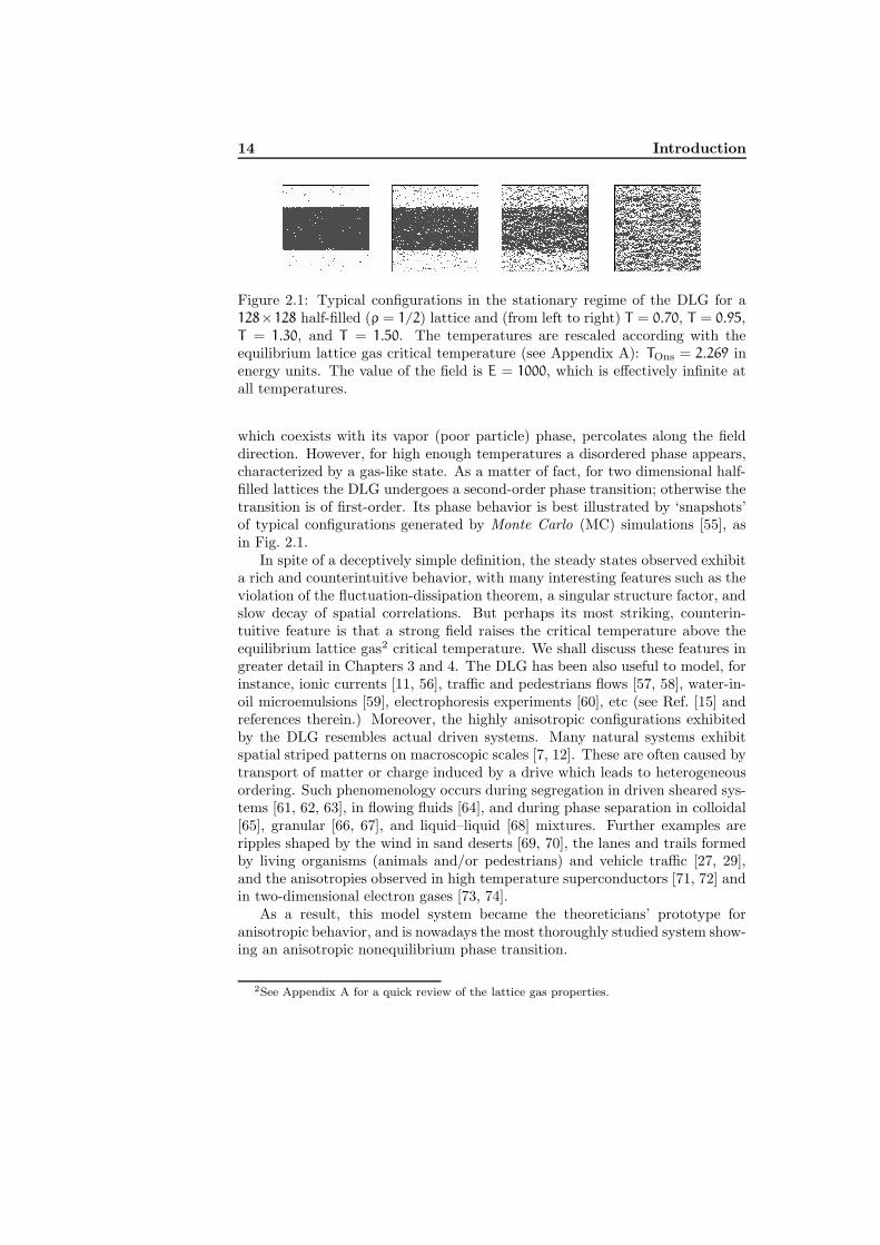
Figure 2.1: Typical configurations in the stationary regime of the DLG for a128×128 half-filled (ρ = 1/2) lattice and (from left to right) T = 0.70, T = 0.95,T = 1.30, and T = 1.50. The temperatures are rescaled according with theequilibrium lattice gas critical temperature (see Appendix A): TOns = 2.269 inenergy units. The value of the field is E = 1000, which is effectively infinite atall temperatures.
which coexists with its vapor (poor particle) phase, percolates along the fielddirection. However, for high enough temperatures a disordered phase appears,characterized by a gas-like state. As a matter of fact, for two dimensional half-filled lattices the DLG undergoes a second-order phase transition; otherwise thetransition is of first-order. Its phase behavior is best illustrated by ‘snapshots’of typical configurations generated by Monte Carlo (MC) simulations [55], asin Fig. 2.1.
In spite of a deceptively simple definition, the steady states observed exhibita rich and counterintuitive behavior, with many interesting features such as theviolation of the fluctuation-dissipation theorem, a singular structure factor, andslow decay of spatial correlations. But perhaps its most striking, counterin-tuitive feature is that a strong field raises the critical temperature above theequilibrium lattice gas2 critical temperature. We shall discuss these features ingreater detail in Chapters 3 and 4. The DLG has been also useful to model, forinstance, ionic currents [11, 56], traffic and pedestrians flows [57, 58], water-in-oil microemulsions [59], electrophoresis experiments [60], etc (see Ref. [15] andreferences therein.) Moreover, the highly anisotropic configurations exhibitedby the DLG resembles actual driven systems. Many natural systems exhibitspatial striped patterns on macroscopic scales [7, 12]. These are often caused bytransport of matter or charge induced by a drive which leads to heterogeneousordering. Such phenomenology occurs during segregation in driven sheared sys-tems [61, 62, 63], in flowing fluids [64], and during phase separation in colloidal[65], granular [66, 67], and liquid–liquid [68] mixtures. Further examples areripples shaped by the wind in sand deserts [69, 70], the lanes and trails formedby living organisms (animals and/or pedestrians) and vehicle traffic [27, 29],and the anisotropies observed in high temperature superconductors [71, 72] andin two-dimensional electron gases [73, 74].
As a result, this model system became the theoreticians’ prototype foranisotropic behavior, and is nowadays the most thoroughly studied system show-ing an anisotropic nonequilibrium phase transition.
2See Appendix A for a quick review of the lattice gas properties.
15
In Chapters 3 and 4 we report on novel findings on this and other relatedmodels by describing different realizations observed in (Metropolis) MC simu-lations. In particular, we study to what extent the DLG features are universal,or in other words, how robust is its behavior. The clue is that the DLG is, in asense, pathological. We also devise a novel driven fluid for anisotropic phenom-ena, which we believe is not only of theoretical importance, but also relevantfor experimentalists. In addition to MC techniques, field-theoretical Langevin-type approaches on the DLG are also developed. But before deep further onthese matters, we shall describe in greater detail the computational and field-theoretical methods employed in these chapters.
In statistical mechanics, Monte Carlo3 simulations [55] play a major roleon the study of phase transitions and critical phenomena. Any MC algorithmgenerates stochastic trajectories in the system’s phase space, in such a waythat the properties of the system are derived from averages over the differenttrajectories. To be specific, for systems both in and far from equilibrium, MCsimulations involve long sequences of configurations, which evolve from one c
to another c′ according to a defined transition probability per unit time (rate),namely, w(c → c′). Once initial transients have decayed stationary observablescan be computed as configurational averages. For systems under equilibriumconditions, such an average over configurations is referred to as the ensembleaverage. In such a case, and if the ergodic hypothesis [3] is assumed, ensembleaverages are equivalent to time averages4.
The acceptance rules for transitions between configurations are chosen suchthat these configurations occur with a frequency prescribed by the desired prob-ability distribution. For equilibrium systems, this must be the “canonical” sta-tionary Gibb’s distribution P0 = e−H/kBT/Z, where H is the Hamiltonian, Z isthe partition function, kB is the Boltzmann’s constant, and T the temperature.Since our interest here is in nonequilibrium behavior, we will need to specifyhow a given configuration c evolves into a new one, c′, that is, w(c → c′).As a consequence, we must deal with a time-dependent probability distributionfunction P(c, t), which obeys a master equation [1, 2]
∂tP(c, t) =∑
c′
P(c′, t) w(c′ → c) − P(c, t) w(c → c′) . (2.1)
Its stationary solution, P(c), controls all the time-independent properties. Toensure that the desired equilibrium distribution P0 is reproduced, one chooses
3More precisely, one should refer it as the Monte Carlo importance sampling algorithm[54, 55]. The nickname “Monte Carlo” comes from the fact that this technique entails a largesequence of random numbers.
4In fact, if MC simulations mimic configurational averages, Molecular Dynamics is a schemefor studying the natural time evolution (time averages) of a certain system. For thermalized(or equilibrated) systems differences between both techniques should disappear in the thermo-
dynamic limit. Chapters 6 and 7 deal with Molecular Dynamic simulations, which are brieflydescribed in Chapter 5.
16 Introduction
rates which satisfy the detailed balance condition, namely
w(c′ → c)
w(c → c′)=
P0(c)
P0(c′). (2.2)
This ensures that the bracket in Eq. (2.1) vanishes. The important point here isthat the ratio P0(c)/P0(c′) = e−∆H/kBT , where ∆H = H(c′) −H(c). One maythus choose rates of the form w(c → c′) = f(∆H/kBT), with an appropriate f
satisfyingf(−x)/f(x) = ex . (2.3)
Some choices for f are the Kawasaki rate f(x) = 2 (1 + ex)−1
[75], the vanBeijeren & Schulman rate f(x) = e−x/2 [76], and the Metropolis rate f(x) =
min 1, e−x [54]. All of our simulations in Part I concern the Metropolis rate.The most simple way of driving a system (as in the DLG case) into a nonequi-
librium steady state is to impose rates that violates detailed balance. A straight-forward extension of ∆H = H(c′)−H(c) in Eq (2.2) is to include the work doneby the field, i.e., to define the total energy difference of the for ∆H + Ex, withx the particle displacement in the field direction. This rate with the propertyEq. (2.3) satisfies the detailed balance condition locally but not globally so thatmicroscopic reversibility of the process as in equilibrium is not guaranteed. Thisscheme is adopted in the DLG which (together with toroidal boundary condi-tions) yields the system towards a nonequilibrium steady state.
It is worth notice that there are recent computational coarse-grained meth-ods, e.g., Dissipative Particle Dynamics (DPD) and Brownian Dynamics (BD)(see for instance [77]), for fluid dynamics which may have several advantagesover conventional computational dynamics methods. The DPD method —firstproposed by Hoogerbrugge and Koelman [78] using heuristic arguments, andproperly formalized by Espanol and Warren [79]— is a useful technique whenstudying the mesoscopic structure of complex liquids. BD is a technique thatresembles DPD but each (mesoscopic) particle feels a random force and a dragforce relative to a fixed background5. However, as we stressed in Chapter 1,we are interested in how the macroscopic behavior emerges from microscopic(atomistic) interactions rather than in modeling the dynamics of fluids from amesoscopic point of view.
Statistical field theories are a complementary approach to the understandingof nonequilibrium ordering in the DLG and in related models. These approachesoften pose great conceptual and computational challenges in themselves, but wewill focus here on critical properties and renormalization group notions throughthe Langevin equation [1, 2]. This is a stochastic partial differential equation,which corresponds to a mesoscopic (coarse-grained) description of the system,and it is thought to describe low-frequency, small-wave number phenomena(such as critical properties). It takes into account only the relevant symmetries
5The important difference between BD and DPD is that BD does not satisfy Newton’sthird law and hence is does not conserve momentum. As a consequence, BD cannot reproducehydrodynamic behavior.
17
for the problem under study and lets the fast degrees of freedom that we forgetabout in the coarse-grained description to act as noise. The Langevin equationfor a field φ takes the following form [1, 2]
∂φ(r, t)
∂t= F[φ] + G[φ]ξ(r, t) , (2.4)
where ξ is a random variable which represents a uncorrelated Gaussian whitenoise. F and G, which are determined in general from symmetry considerations,are analytic functionals of φ. In fact, these functionals include every analyticterm consistent with the symmetries of the microscopic system. In principle,F and G can be determined phenomenologically through experiments and/orsymmetry arguments. Other difficult procedure which is seldom carried outis the coarse-graining operation that produces the Langevin equation from themicroscopic model, which follows, say, a master equation as Eq. (2.1). We adoptthe latter procedure (we extend the scheme devised in Ref. [80]) in the Chapter 3and in greater detail in the Appendix C.
18 Introduction
Chapter 3
Lennard–Jones and Lattice
models of driven fluids
The present chapter describes Monte Carlo (MC) simulations and field theoret-ical calculations that aim at illustrating how slight modifications of dynamics atthe microscopic level may influence, even quantitatively, the resulting (nonequi-librium) steady state. With this aim, we take as a reference the driven lattice gas(DLG), which we described qualitatively in the previous chapter. We presentand study related lattice and off-lattice microscopic models in which particles,as in the DLG, interact via a local anisotropic rule. The rule induces preferentialhopping along one direction, so that a net current sets in if allowed by bound-ary conditions. In particular, we shall discuss on the similarities and differencesbetween the DLG and its continuous counterpart, namely, a Lennard–Jonesanalogue in which the particles’ coordinates vary continuously. A comparisonbetween the two models allows us to discuss some exceptional, hardly realisticfeatures of the original discrete system —which has been considered a prototypefor nonequilibrium anisotropic phase transitions.
3.1 Driven Lattice Gas
The driven lattice gas [53] is a nonequilibrium extension of the Ising model withconserved dynamics. The DLG consists of a d-dimensional square lattice gasin which pair of particles interact via an attractive and short–range Ising–likeHamiltonian,
H = −4∑
〈j,k〉σjσk . (3.1)
Here σk is the lattice occupation number at site k ∈ Zd, and the sum runs overall the nearest-neighbor (NN) sites1. Each lattice site has two possible states,namely, a particle (σk = 1) or a hole (σk = 0) may occupy each site k. Cell
1For d = 2, this corresponds with a lattice’s connectivity 4.
20 Lennard–Jones and Lattice models of driven fluids
dimensions for the lattice are chosen so that the NN distance (bond length) wasunity: |j−k| = 1. A configuration is given by σ ≡ σk ; k ∈ d-dimensional lattice.We shall restrict ourselves to two-dimensional L‖ × L⊥ lattices, that is, d = 2.Dynamics is induced by the competion between a heat bath at temperatureT and an external driving field E which favors particle hops along one of theprincipal lattice directions, say horizontally (x direction), as if the particles werepositively charged. Consequently, for periodic boundary conditions, a nontrivialnonequilibrium steady state is set in asymptotically. This is formalized througha master equation similar to Eq. (2.1), where the transition probabilities perunit time w(σ → σ′) are the Metropolis ones, namely,
w(σ → σ′) = min1, e−(∆H+E·δ)/(kBT)
. (3.2)
Where E ·δ denotes the dot product between the field E (oriented along x direc-tion) and δ, which is the attempted particle displacement, i.e, δ = (j − k)(σj −
σk); and ∆H = H(σ′) − H(σ). To be precise, w(σ → σ′) stands for the ratefor the particle-hole exchange σk σj when the configuration is σ; the par-ticle density ρ = N/(L‖L⊥) remains constant during the time evolution. Theexchange σk σj corresponds to a particle jumping to a NN hole if σk 6= σj;we assume w(σ → σ′) = 0 otherwise, i.e., only NN particle-hole exchanges areallowed. This bias breaks detailed balance and establishes a nonequilibriumsteady state. Typical configurations in the stationary regime of the DLG areshown in Fig. 2.1.
MC simulations by the biased Metropolis rate in Eq. (3.2) reveal that, asin equilibrium, the DLG undergoes a second order phase transition. At highenough temperature, the system is in a disordered state while, below a criticalpoint (at T ≤ TE, where E = |E|) it orders displaying anisotropic phase segre-gation. That is, an striped rich–particle phase then coexists with its gas. It isalso found that, for a lattice half filled of particles, the critical temperature TE
monotonically increases with E from the Onsager value2 T0 = TOns = 2.269 Jk−1B
to T∞ ' 1.4 TOns. This limit (E → ∞) corresponds to a nonequilibrium criticalpoint. As a matter of fact, it was numerically shown to belong to a universalityclass other than the Onsager one, e.g., MC data indicates βDLG ' 0.33 (insteadof the Ising value β = 1/8 in two dimensions) for the order parameter criticalexponent [11, 81, 82]. Typical configurations for the DLG in the large field limitwere shown in Fig. 2.1.
Statistical field theory is a complementary approach to the understandingof nonequilibrium ordering in the DLG. The derivation of a general mesoscopicdescription is still an open issue, however. Two different approaches have beenproposed. The driven diffusive system (DDS) [15, 83, 84], which is a phenomeno-logical Langevin-type equation aimed at capturing all the relevant symmetries,predicts that the current will induce a predominant mean–field behavior and,in particular, βDDS = 1/2. The anisotropic diffusive system (ADS) [80], which
2See Appendix A.
3.1 Driven Lattice Gas 21
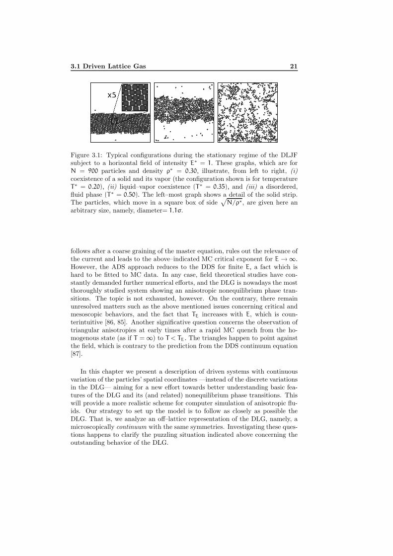
Figure 3.1: Typical configurations during the stationary regime of the DLJFsubject to a horizontal field of intensity E∗ = 1. These graphs, which are forN = 900 particles and density ρ∗ = 0.30, illustrate, from left to right, (i)coexistence of a solid and its vapor (the configuration shown is for temperatureT∗ = 0.20), (ii) liquid–vapor coexistence (T ∗ = 0.35), and (iii) a disordered,fluid phase (T∗ = 0.50). The left–most graph shows a detail of the solid strip.The particles, which move in a square box of side
√
N/ρ∗, are given here anarbitrary size, namely, diameter= 1.1σ.
follows after a coarse graining of the master equation, rules out the relevance ofthe current and leads to the above–indicated MC critical exponent for E → ∞.
However, the ADS approach reduces to the DDS for finite E, a fact which ishard to be fitted to MC data. In any case, field theoretical studies have con-stantly demanded further numerical efforts, and the DLG is nowadays the mostthoroughly studied system showing an anisotropic nonequilibrium phase tran-sitions. The topic is not exhausted, however. On the contrary, there remainunresolved matters such as the above mentioned issues concerning critical andmesoscopic behaviors, and the fact that TE increases with E, which is coun-terintuitive [86, 85]. Another significative question concerns the observation oftriangular anisotropies at early times after a rapid MC quench from the ho-mogenous state (as if T = ∞) to T < TE. The triangles happen to point againstthe field, which is contrary to the prediction from the DDS continuum equation[87].
In this chapter we present a description of driven systems with continuousvariation of the particles’ spatial coordinates —instead of the discrete variationsin the DLG— aiming for a new effort towards better understanding basic fea-tures of the DLG and its (and related) nonequilibrium phase transitions. Thiswill provide a more realistic scheme for computer simulation of anisotropic flu-ids. Our strategy to set up the model is to follow as closely as possible theDLG. That is, we analyze an off–lattice representation of the DLG, namely, amicroscopically continuum with the same symmetries. Investigating these ques-tions happens to clarify the puzzling situation indicated above concerning theoutstanding behavior of the DLG.
22 Lennard–Jones and Lattice models of driven fluids
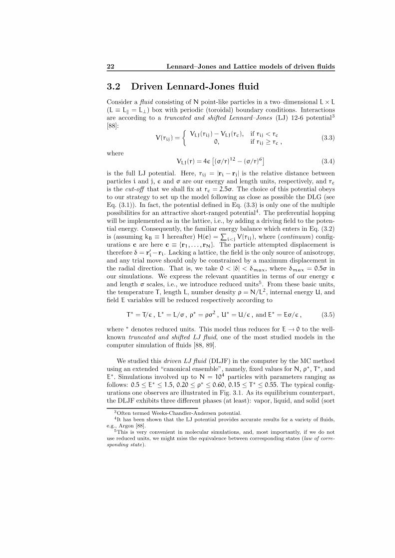
3.2 Driven Lennard-Jones fluid
Consider a fluid consisting of N point-like particles in a two–dimensional L× L
(L ≡ L‖ = L⊥) box with periodic (toroidal) boundary conditions. Interactionsare according to a truncated and shifted Lennard–Jones (LJ) 12-6 potential3
[88]:
V(rij) =
VLJ(rij) − VLJ(rc), if rij < rc
0, if rij ≥ rc ,(3.3)
whereVLJ(r) = 4ε
[
(σ/r)12 − (σ/r)6]
(3.4)
is the full LJ potential. Here, rij = |ri − rj| is the relative distance betweenparticles i and j, ε and σ are our energy and length units, respectively, and rc
is the cut-off that we shall fix at rc = 2.5σ. The choice of this potential obeysto our strategy to set up the model following as close as possible the DLG (seeEq. (3.1)). In fact, the potential defined in Eq. (3.3) is only one of the multiplepossibilities for an attractive short-ranged potential4. The preferential hoppingwill be implemented as in the lattice, i.e., by adding a driving field to the poten-tial energy. Consequently, the familiar energy balance which enters in Eq. (3.2)is (assuming kB ≡ 1 hereafter) H(c) =
∑i<j V(rij), where (continuum) config-
urations c are here c ≡ r1, . . . , rN. The particle attempted displacement istherefore δ = r′i −ri. Lacking a lattice, the field is the only source of anisotropy,and any trial move should only be constrained by a maximum displacement inthe radial direction. That is, we take 0 < |δ| < δmax, where δmax = 0.5σ inour simulations. We express the relevant quantities in terms of our energy ε
and length σ scales, i.e., we introduce reduced units5. From these basic units,the temperature T , length L, number density ρ = N/L2, internal energy U, andfield E variables will be reduced respectively according to
T∗ = T/ε , L∗ = L/σ , ρ∗ = ρσ2 , U∗ = U/ε , and E∗ = Eσ/ε , (3.5)
where ∗ denotes reduced units. This model thus reduces for E → 0 to the well-known truncated and shifted LJ fluid, one of the most studied models in thecomputer simulation of fluids [88, 89].
We studied this driven LJ fluid (DLJF) in the computer by the MC methodusing an extended “canonical ensemble”, namely, fixed values for N, ρ∗, T∗, andE∗. Simulations involved up to N = 104 particles with parameters ranging asfollows: 0.5 ≤ E∗ ≤ 1.5, 0.20 ≤ ρ∗ ≤ 0.60, 0.15 ≤ T∗ ≤ 0.55. The typical config-urations one observes are illustrated in Fig. 3.1. As its equilibrium counterpart,the DLJF exhibits three different phases (at least): vapor, liquid, and solid (sort
3Often termed Weeks-Chandler-Andersen potential.4It has been shown that the LJ potential provides accurate results for a variety of fluids,
e.g., Argon [88].5This is very convenient in molecular simulations, and, most importantly, if we do not
use reduced units, we might miss the equivalence between corresponding states (law of corre-
sponding state).
3.2 Driven Lennard-Jones fluid 23
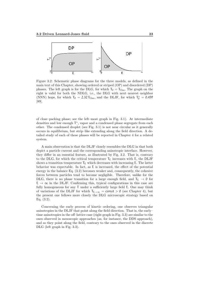
Figure 3.2: Schematic phase diagrams for the three models, as defined in themain text of this Chapter, showing ordered or striped (OP) and disordered (DP)phases. The left graph is for the DLG, for which T0 = TOns. The graph on theright is valid for both the NDLG, i.e., the DLG with next–nearest–neighbor(NNN) hops, for which T0 = 2.32 TOns, and the DLJF, for which T∗
0 = 0.459
[89].
of close–packing phase; see the left–most graph in Fig. 3.1). At intermediatedensities and low enough T∗, vapor and a condensed phase segregate from eachother. The condensed droplet (see Fig. 3.1) is not near circular as it generallyoccurs in equilibrium, but strip–like extending along the field direction. A de-tailed study of each of these phases will be reported in Chapter 4 for a relatedsystem.
A main observation is that the DLJF closely resembles the DLG in that bothdepict a particle current and the corresponding anisotropic interface. However,they differ in an essential feature, as illustrated by Fig. 3.2. That is, contraryto the DLG, for which the critical temperature TE increases with E, the DLJFshows a transition temperature TE which decreases with increasing E. The latterbehavior was expectable. In fact, as E is increased, the effect of the potentialenergy in the balance Eq. (3.2) becomes weaker and, consequently, the cohesiveforces between particles tend to become negligible. Therefore, unlike for theDLG, there is no phase transition for a large enough field, and TE → 0 forE → ∞ in the DLJF. Confirming this, typical configurations in this case arefully homogeneous for any T under a sufficiently large field E. One may thinkof variations of the DLJF for which TE→∞ = const > 0 (see Chapter 4), butthe present one follows more closely the DLG microscopic strategy based onEq. (3.2).
Concerning the early process of kinetic ordering, one observes triangularanisotropies in the DLJF that point along the field direction. That is, the early–time anisotropies in the off–lattice case (right graph in Fig. 3.3) are similar to theones observed in mesoscopic approaches (as, for instance, the DDS approach),and so they point along the field, contrary to the ones observed in the discreteDLG (left graph in Fig. 3.3).

24 Lennard–Jones and Lattice models of driven fluids
Figure 3.3: Triangular anisotropies as observed at early times for E = 1 in com-puter simulations of the lattice (left) and the off–lattice (right) models definedin the main text. The field points along the x direction. The DLG configurationis for t = 6 × 10⁴ MC steps in a 128×128 lattice with N = 7372 particles andT = 0.4TOnsager. The DLJF configuration is for t = 1.5×10⁵ MC steps, N = 104
particles, ρ∗ = 0.20 and T∗ = 0.23.
3.3 Driven Lattice Gas with extended dynamics
The above observations altogether suggest a unique exceptionality of the DLGbehavior. This is to be associated with the fact that a driven particle is geo-metrically restrained in the DLG. In order to show this, we studied the latticewith an infinite drive extending the hopping to next–nearest–neighbors (NNN)[90, 91, 92]. That is, we extend interactions and accessible sites to the NNN.Thus, the sum in Eq. (3.1) involves the eight next-nearest neighbors instead ofthe four nearest neighbors of the standard DLG. In this case, the particle-holeexchange σk σj corresponds to a particle hop to a NNN hole if σk 6= σj. Asillustrated in Fig. 3.4, this introduces further relevant directions in the lattice,so that the resulting model, to be named here NDLG, is expected to behavecloser to the DLJF. This is confirmed. For example, one observes in the dis-crete NDLG that, as in the continuum DLJF, TE decreases with increasing E
—though from T0 = 2.32 TOns in this case6—. This is illustrated in Fig. 3.2.Specifically, we discuss on this difference between the DLG and the NDLG inAppendix B, in where we define an intermediate model which capture bothsituations.
3.3.1 Correlations and Structure Factor
There is also interesting information in the two–point correlation function and(equal-time) structure factor. The former, which measures the degree of orderof the lattice, is defined for a half–filled lattice as
C(i) = 〈σj σi+j〉 − 1/4, (3.6)
6For the Ising model with NNN interactions, one can derive easily theoretical estimates forthe critical temperature [94].
3.3 Driven Lattice Gas with extended dynamics 25
NN hops NNN hopsE=0
T
ET x
T x
x
xT
T
T
T
T
TT
T
T T T
T
T
E
E
E
NN hops NNN hopsE=∞
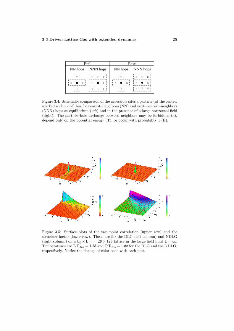
Figure 3.4: Schematic comparison of the accessible sites a particle (at the center,marked with a dot) has for nearest–neighbors (NN) and next–nearest–neighbors(NNN) hops at equilibrium (left) and in the presence of a large horizontal field(right). The particle–hole exchange between neighbors may be forbidden (x),depend only on the potential energy (T), or occur with probability 1 (E).
Figure 3.5: Surface plots of the two–point correlation (upper row) and thestructure factor (lower row). These are for the DLG (left column) and NDLG(right column) on a L‖ × L⊥ = 128 × 128 lattice in the large field limit E = ∞.Temperatures are T/TOns = 1.58 and T/TOns = 1.00 for the DLG and the NDLG,respectively. Notice the change of color code with each plot.
26 Lennard–Jones and Lattice models of driven fluids
0 5 10 15 20 25x,y
0
0.1
0.2
0.3
C||, C
⊥1 10x
10-4
10-2
C||
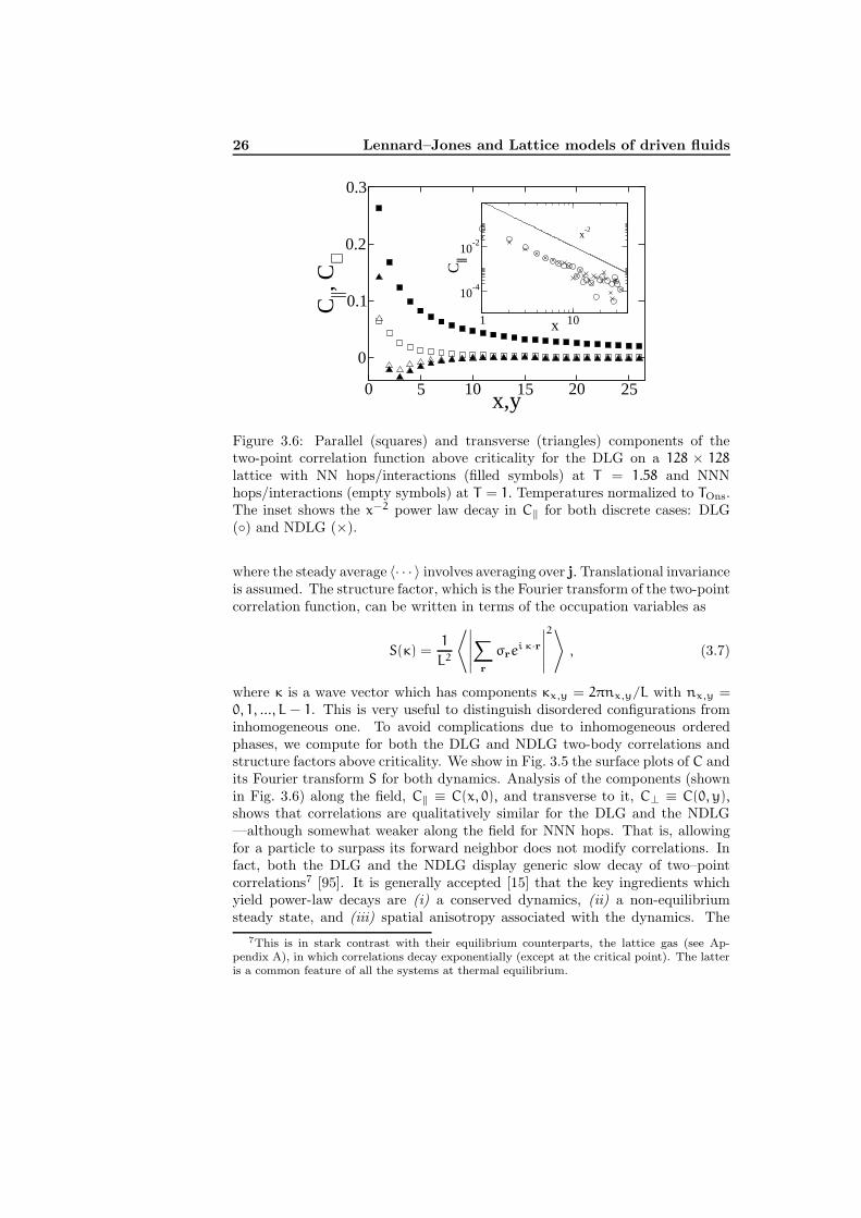
x-2
Figure 3.6: Parallel (squares) and transverse (triangles) components of thetwo-point correlation function above criticality for the DLG on a 128 × 128
lattice with NN hops/interactions (filled symbols) at T = 1.58 and NNNhops/interactions (empty symbols) at T = 1. Temperatures normalized to TOns.The inset shows the x−2 power law decay in C‖ for both discrete cases: DLG() and NDLG (×).
where the steady average 〈· · · 〉 involves averaging over j. Translational invarianceis assumed. The structure factor, which is the Fourier transform of the two-pointcorrelation function, can be written in terms of the occupation variables as
S(κ) =1
L2
⟨∣
∣
∣
∣
∣
∑
r
σrei κ·r
∣
∣
∣
∣
∣
2⟩
, (3.7)
where κ is a wave vector which has components κx,y = 2πnx,y/L with nx,y =
0, 1, ..., L − 1. This is very useful to distinguish disordered configurations frominhomogeneous one. To avoid complications due to inhomogeneous orderedphases, we compute for both the DLG and NDLG two-body correlations andstructure factors above criticality. We show in Fig. 3.5 the surface plots of C andits Fourier transform S for both dynamics. Analysis of the components (shownin Fig. 3.6) along the field, C‖ ≡ C(x, 0), and transverse to it, C⊥ ≡ C(0, y),
shows that correlations are qualitatively similar for the DLG and the NDLG—although somewhat weaker along the field for NNN hops. That is, allowingfor a particle to surpass its forward neighbor does not modify correlations. Infact, both the DLG and the NDLG display generic slow decay of two–pointcorrelations7 [95]. It is generally accepted [15] that the key ingredients whichyield power-law decays are (i) a conserved dynamics, (ii) a non-equilibriumsteady state, and (iii) spatial anisotropy associated with the dynamics. The
7This is in stark contrast with their equilibrium counterparts, the lattice gas (see Ap-pendix A), in which correlations decay exponentially (except at the critical point). The latteris a common feature of all the systems at thermal equilibrium.

3.3 Driven Lattice Gas with extended dynamics 27
0 5 10 15 20n
x,n
y
5
10
15
S ||, S⊥
1
2
3
Figure 3.7: Parallel (squares) and transverse (triangles) components of the struc-ture factor above criticality for the DLG on a 128 × 128 lattice for the DLG(filled symbols, left scale) at T = 1.58 and for the NDLG (empty symbols, rightscale) at T = 1. Temperatures normalized to TOnsager. Here, nx,y = 128 κx,y/2π.
first ingredient alone (as in equilibrium) cannot lead to generic power laws dueto the validity of the fluctuation dissipation theorem. The role of the secondingredient is to lift the theorem’s constraint, so that the power laws are nowgeneric. The role of the third one is more subtle, necessary only for producingpower laws in the two-body correlations.
The power-law behavior8 translates into a discontinuity of the structure fac-tor, namely, limκx→0 S‖ 6= limκy→0 S⊥, where S‖ ≡ S(κx, 0) and S⊥ ≡ S(0, κy).This is clearly confirmed in Fig. 3.7 for both NN and NNN hops/interactions.Notice that this singularity, which do not appear under equilibrium conditions,is an indication of the dependence of the nonequilibrium steady state on the(anisotropic) dynamic.
3.3.2 Critical behavior
As outlined in Section 3.1, the derivation of a general mesoscopic description isstill an issue under contention. In order to shed more light on the field theoreticaldescription of driven fluids, we try to derive a Langevin-type equation for theNDLG. To this end, firstly, we compute the order parameter critical exponentby means of standard finite size scaling techniques. Secondly, we derive theLangevin equation, which aim at describe the NDLG critical properties, byusing the ADS approach [80]. We also discuss the viability of other approaches,e.g., the DDS approach.
8Together with the Ising symmetry violation by E 6= 0.
28 Lennard–Jones and Lattice models of driven fluids
MC simulations
Assuming a half–filled lattice9 we perform finite size scaling analysis for theNDLG by following the scheme proposed in [15] consistent with the ADS theory[81]. The order parameter is chosen as the structure factor
m = S(0, 2π/L⊥) , (3.8)
(as suggested in [96, 97, 98]), which carries the intrinsic anisotropies of thesystem. In order to perform systematic anisotropic finite size scaling we con-sidered system sizes 80 × 40, 25 × 50, 45 × 30, and 125 × 50. These aspect
ratios satisfy Lν⊥/ν‖
‖ = 0.22 × L⊥, where ν⊥/ν‖ ≈ 1/2 consistent with the ADS
anisotropic spatial scaling [96, 97, 98]. A strong enough field is needed to avoidcrossovers from the equilibrium regime. Notice also that, as we showed abovefor the NDLG, a saturating field suppresses the ordering, that is, TE = 0 whenE → ∞. Therefore we choose an intermediate value for the field E = 12. Thecorresponding critical temperature is determined by using the Binder’s fourthcumulant method [99], which is T12 = 1.45 ± 0.01. The obtained critical valueT12 was employed for the finite size scaling analysis.
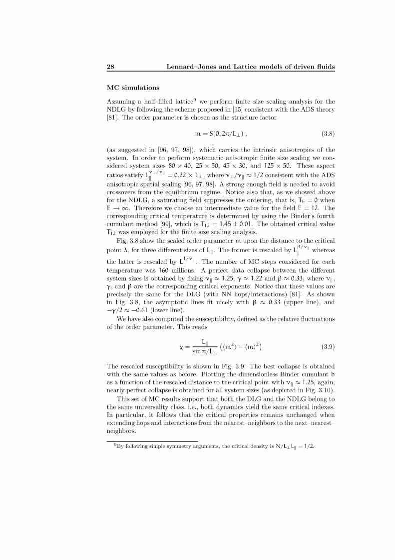
Fig. 3.8 show the scaled order parameter m upon the distance to the critical
point λ, for three different sizes of L‖. The former is rescaled by Lβ/ν‖
‖ whereas
the latter is rescaled by L1/ν‖
‖ . The number of MC steps considered for each
temperature was 160 millions. A perfect data collapse between the differentsystem sizes is obtained by fixing ν‖ ≈ 1.25, γ ≈ 1.22 and β ≈ 0.33, where ν‖,γ, and β are the corresponding critical exponents. Notice that these values areprecisely the same for the DLG (with NN hops/interactions) [81]. As shownin Fig. 3.8, the asymptotic lines fit nicely with β ≈ 0.33 (upper line), and−γ/2 ≈ −0.61 (lower line).
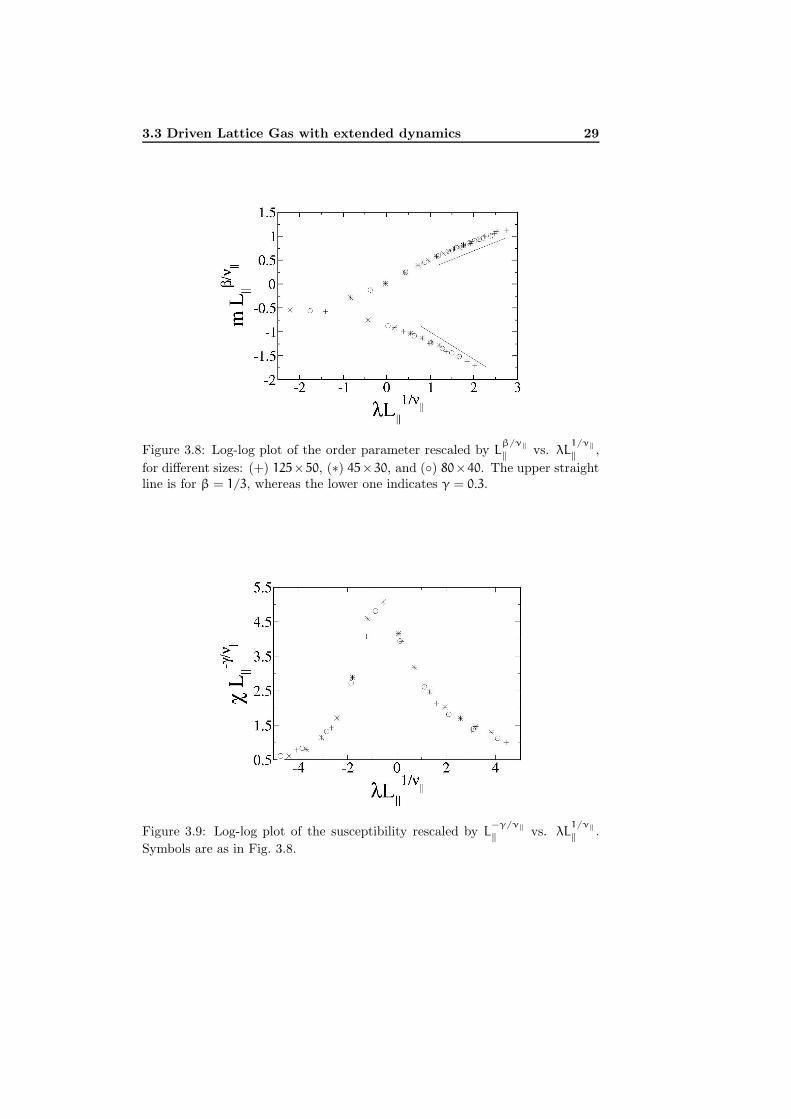
We have also computed the susceptibility, defined as the relative fluctuationsof the order parameter. This reads
χ =L‖
sin π/L⊥
(
〈m2〉 − 〈m〉2)
(3.9)
The rescaled susceptibility is shown in Fig. 3.9. The best collapse is obtainedwith the same values as before. Plotting the dimensionless Binder cumulant b
as a function of the rescaled distance to the critical point with ν‖ ≈ 1.25, again,nearly perfect collapse is obtained for all system sizes (as depicted in Fig. 3.10).
This set of MC results support that both the DLG and the NDLG belong tothe same universality class, i.e., both dynamics yield the same critical indexes.In particular, it follows that the critical properties remains unchanged whenextending hops and interactions from the nearest–neighbors to the next–nearest–neighbors.
9By following simple symmetry arguments, the critical density is N/L⊥L‖ = 1/2.
3.3 Driven Lattice Gas with extended dynamics 29
Figure 3.8: Log-log plot of the order parameter rescaled by Lβ/ν‖
‖ vs. λL1/ν‖
‖ ,
for different sizes: (+) 125×50, (∗) 45×30, and () 80×40. The upper straightline is for β = 1/3, whereas the lower one indicates γ = 0.3.
Figure 3.9: Log-log plot of the susceptibility rescaled by L−γ/ν‖
‖ vs. λL1/ν‖
‖ .
Symbols are as in Fig. 3.8.

30 Lennard–Jones and Lattice models of driven fluids
Figure 3.10: Scaling plot of the fourth Binder cumulant b vs. λL1/ν‖
‖ . Symbolsare as in Fig. 3.8.
Mesoscopic description
The ADS approach has been employed successfully to describe the critical be-havior of the DLG [80]. The resulting Langevin–type equation, derived froma coarse–graining process from the DLG master (microscopic) equation sets upthe anisotropy as the main nonequilibrium ingredient and leads to the rightcritical exponent in the large field limit (β ≈ 1/3). The associated Langevinequation for the coarse–grained density φ(r, t) reads
∂tφ(r, t) = −∇4⊥φ + (τ + a)∇2
⊥φ +g
3!∇2
⊥φ3 +a
2∇2
‖φ + ξ(r, t) (3.10)
Here, the last term ξ stands for a Gaussian white noise, i.e., 〈ξ(r, t)〉 = 0 and〈ξ(r, t)ξ(r′, t′)〉 = δ(r − r′)δ(t − t′), representing the fast degrees of freedom,and τ, a and g are model parameters.
This approach is certainly valuable because it represents a detailed connec-tion between microscopic dynamics and their mesoscopic descriptions. There-fore, this important feature suggests that its validity can be extended to describethe critical behavior of the NDLG, which was studied by computational meansin the previous subsection. Such a description include the microscopic details ofdiagonal dynamics which, in particular, should allow us to distinguish betweenthe DLG and the NDLG. This is in contrast of other more heuristic approaches,as the DDS [15, 83, 84], which aim for the main symmetries of the DLG. TheDDS approach is the natural extension of the conserved φ4 theory for the Isingequilibrium model [100]. The most relevant prediction of the DDS is the meanfield behavior β = 1/2, which conflicts with MC simulations. This is not sur-prising, because the DLG behavior is more complicated than its equilibriumcounterpart, in which the symmetries and the influence of the dynamics is well

3.3 Driven Lattice Gas with extended dynamics 31
established. The same situation occurs when extending dynamics to the NNN:the DDS (heuristic) scheme leads again to the mean–field order parameter crit-ical exponent. As a matter of fact, the DDS approach can not account forthe diagonal (microscopic) degrees of freedom. Therefore, the DDS Langevinequation does not describe the NDLG critical properties.
The question is whether the ADS approach describes properly the criticalbehavior observed in the NDLG. This is addressed in this section.
Next, we outline the derivation of a Langevin equation for the NDLG byfollowing the scheme proposed in [80]. (this derivation can be found in greaterdetail in Appendix C).
Let us define a density variable φ(r, t) averaged in a region of volume v overwhich the original microscopic occupation variable (σk in Eq. (3.1)) were aver-aged. The system evolves from a (coarse–grained) configuration γ to anotherγ′ by choosing randomly a particle at point r and exchanging it with one ofits next nearest neighbors in the direction µ [80]. Notice that, in contrast withthe previous ADS approach for the DLG with NN interactions, now µ involvesthe known parallel ‖ and transversal ⊥ directions as well as the two additionaldirections which allow for the diagonal jumps and . If v is large enough,then φ can be considered a continuum function of r so we have
γ′ =φ + v−1 ∇µδ(r′ − r), where φ ∈ γ
(3.11)
The distribution P(γ, t) accounts for the statistical weight of each configurationγ at time t and evolves according to the following Markovian master equation[1]
∂tP(γ, t) =∑
µ=‖,⊥,,
∫
dηf(η)
∫
dr [Ω(γ → γ′)P(γ, t) − Ω(γ′ → γ)P(γ′, t)]
(3.12)where Ω(γ → γ′) stands for the transition probability per unit time (transitionrate) from γ to γ′ and f(η) is an even function which account for the amount ofmass attempted to be displaced. That is, Eq. (3.11)–(3.12) represent a proccessin which a configuration γ is exchanged with the infinitesimal neighbor of r (γ′)in the µ direction. As usual, the transition rates are taken to be a product ofa function of the entropy times the same function of the difference between theconfigurations plus a term due to the effect of the driving field [33], namely,
Ω(γ → γ′) = D(∆S(η)) · D(∆H(η) + Hε). (3.13)
Here, Hε = η µ · ε (1 − φ2) + O(v−1), and D is a function satisfying detailedbalance. Importantly, in the Langevin–type equations framework, ε representsa coarse–grained field acting upon a given configuration η. Indeed, the detaileddependence of the mesoscopic coefficients on the microscopic field introducedin Eq. (3.2) remain still as an open issue [11]. This constraint ensures thatthe limiting case of ε = 0 the steady state solution of the master equation isthe canonical one, i.e. P(γ, t = ∞)|ε=0 = e−H[φ]. At a mesoscopic level, the
32 Lennard–Jones and Lattice models of driven fluids
equivalent to Eq. (3.1) is the standard φ4 (Ginzburg–Landau) Hamiltonian,and following a similar procedure as here the equilibrium Langevin equation isthe so called model B [100]. The structure of the free energy consist of twocontributions: a entropic and a energetic one which are given by, respectively
S(η) = v
∫
dr(a
2φ2 +
g
4!φ4
)
H(η) = v
∫
dr
(
1
2(∇φ)
2+
τ
2
)
. (3.14)
Here a and g are entropic coefficients whereas the parameter τ comes from theenergetic contribution. From Eq. (3.12) a Fokker–Planck equation is derivedby means of a Kramers–Moyal [1] expansion. The derivation is similar to theone in Ref. [80], but taking into account the transversal degrees of freedomfor the NDLG. After using standard techniques in the theory of stochastic pro-cesses [1] we derive from the Fokker–Planck equation its stochastically equivalentLangevin equation using the Ito prescription, which reads
∂tφ(r, t) =∑
µ
∇µ
[
p(λSµ, λH
µ + λεµ) + q(λS
µ, λHµ + λε
µ)1/2ξµ(r, t)]
. (3.15)
where
λεµ = µ · ε (1 − φ2),
λXµ = −
(
∇µ
δ
δφ
)
X,
p(z1, z2) =
∫
dr η f(η) D(ηz1) D(ηz2),
q(z1, z2) =
∫
dr η2 f(η) D(ηz1) D(ηz2). (3.16)
The time has been rescaled by v−1 and ξµ(r, t) is a delta–correlated Gaussianwhite noise in the µ direction. After some algebra, the terms depending on bothdiagonal components and can be split into the two parallel and transversalto the field components. We now focus on the critical region and discard irrel-evant terms in the renormalization group sense by naive power counting. Weperform the following anisotropic scale transformations:
t → τ−zt ,
r⊥ → τ−1r⊥ ,
r‖ → τ−sr‖ ,
φ → τδφ .
(3.17)
Expanding the Langevin equation Eq. (3.15) around τ = 0 keeping only themore relevant terms, we found that the leading terms of the theory are ∇4
⊥φ and∇2
‖φ which, together with imposing invariance of the time scale, the transverse

3.4 Conclusions 33
spatial interaction, and the transverse noise, under scale transformations, leadto s = 2, δ = (s + d − 3)/2, and z = 4. According to this and after somecumbersome algebra, the Langevin equation for finite (coarse–grained) drivingfield contains a large bunch of field–dependent terms. Similarly to what occursin the ADS approach for the DLG, just taking a large enough value of the fieldmost of those terms vanish. By doing this, one is led to the following Langevinequation
∂tφ(r, t) = −∇4⊥φ + (τ +
3
2a)∇2
⊥φ +g
4∇2
⊥φ3 + a∇2‖φ + ξ(r, t) (3.18)
The resulting equation resemble the one for NN interactions (see Eq. (3.10)),although in Eq. (3.18) appears additional prefactors of entropic nature. This isconsistent with the fact that the model with the extended dynamics, i.e., theNDLG, possesses more neighbors than the DLG. The present equation for NNNinteractions contains all the same symmetries as Eq. (3.10) and both lead to thesame critical behavior. The value of the order parameter critical exponent thatfollows from a renormalization group analysis of Eq. (3.18) is β = 1/3, which isconsistent with the observed in the MC simulations described above.
3.4 Conclusions
The above observations show that the nature of correlations is not enough todetermine the phase diagram. There are already indications of this from thestudy of equilibrium systems, and also from other nonequilibrium models. Thatis, one may have a qualitatively different phase diagram but essentially thesame two–point correlations by modifying the microscopic dynamics. It follows,in particular, that the exceptional behavior of the DLG cannot be understoodjust by invoking the two-point correlation function C(i) —or, equivalently, thestructure factor S(κ)— or crude arguments concerning symmetries. The factthat particles are constrained to travel precisely along the two principal latticedirections in the DLG is the cause for its singular behavior. Or in other words,the lattice geometry acts more efficiently in the DLG as an ordering agent thanthe field itself, which occurs rarely in actual cooperative transport in fluids.This means that the ordering in the DLG is a geometric effect rather thandynamic. Allowing jumping along intermediate directions, as in both the NDLGand the DLJF, modifies essentially the phase diagram but not features —suchas power–law correlations— that seem intrinsic of the nonequilibrium natureof the phenomenon. This special arrangement of particles is also lacking, forinstance, when other orientations of the driving field [101] are considered. Thisalso would explain certain irregular configurations observed in three dimensions[11], since this constraint is also lifted in the d = 3 case.
Rutenberg and Yeung [92] also performed quenching experiments for varia-tions of the DLG10. They showed, in particular, that minor modifications in the
10They allow for NNN hops, but the Hamiltonian only involves the NN interactions.
34 Lennard–Jones and Lattice models of driven fluids
DLG dynamics may lead to an inversion of the triangular anisotropies duringthe formation of clusters which finally condense into strips. Our observationsabove prove that such nonuniversal behavior goes beyond kinetics, namely, italso applies to the stationary state.
The unique exceptionality of the DLG has some important consequences.One is that this model involves features that are not frequent in nature. Thereare situations in which a drive induces stripes but not necessarily DLG behavior[61]. The fact that a particle impedes the freedom of the one behind to movealong x for a large enough field may only occur very seldom in cooperative trans-port in fluids. The NDLG is more realistic in this sense. In any case, the greateffort devoted to the DLG during two decades has revealed important proper-ties of both nonequilibrium steady states and anisotropic phase transitions. Onthe other hand, it ensues that, due to its uniqueness, the DLG does not havea simple off-lattice analog. This is because the ordering agent in the DLG ismore the lattice geometry than the field itself. The fact that one needs to bevery careful when modeling nonequilibrium phenomena —one may induce botha wrong critical behavior and an spurious phase diagram— ensues again in thisexample. This seems not to be so dramatic in equilibrium where, for example,the lattice gas is a useful oversimplification of a LJ fluid.
Concerning criticality, according to our observations we found that the aniso-tropic diffusive system approach include the microscopic details of transversedynamics which, in particular, allow one to distinguish between the DLG andthe NDLG. This is in contrast with other, more heuristic approaches, e.g., thedriven diffusive system. The ADS approach lead to the right order parametercritical exponent given by MC simulations. We analyzed the order parameter,magnetization, and the fourth Binder cumulant in order to compute the criticalexponents. By using anisotropic finite size scaling we have shown that, in spiteof structural differences between them, both models belong to the same uni-versality class, which is characterized by an order parameter critical exponentβ ≈ 1/3.
Consequently, their critical properties do not depend on this particular ex-tension of the dynamics. There are other nonequilibrium models in which thecorresponding critical behavior changes by such an extension of the dynamicfrom NN to NNN. This is, for instance, the case of a closely related latticesystem (with NN exclusion under a driving field) devised by Dickman [93]: Ex-tending the dynamics to NNN [91], the nature of the order–disorder transitionwhich takes place in this model changes dramatically. We shall discuss furtheron this model in the next chapter.
Finally, we remark that in the novel fluid model introduced in this chapter,the particle ‘infinite freedom’ is realistic, as it is also the LJ potential. It maycontain some of the essential physics in a class of nonequilibrium anisotropic phe-nomena and phase transitions. On the other hand, the model is simple enoughto be useful in computer simulations, and it is endowed of even–simpler andfunctional lattice analogs such as the NDLG. In the following chapter (Chap-ter 4) we shall develop in greater detail this matter.
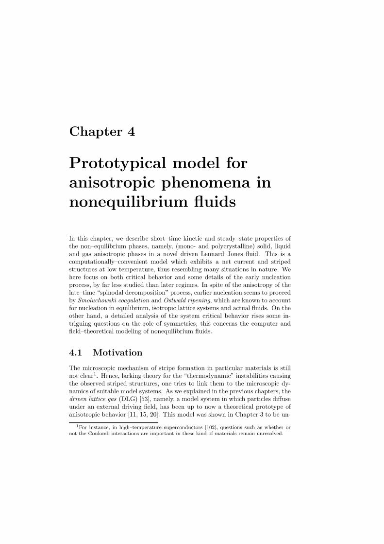
Chapter 4
Prototypical model for
anisotropic phenomena in
nonequilibrium fluids
In this chapter, we describe short–time kinetic and steady–state properties ofthe non–equilibrium phases, namely, (mono- and polycrystalline) solid, liquidand gas anisotropic phases in a novel driven Lennard–Jones fluid. This is acomputationally–convenient model which exhibits a net current and stripedstructures at low temperature, thus resembling many situations in nature. Wehere focus on both critical behavior and some details of the early nucleationprocess, by far less studied than later regimes. In spite of the anisotropy of thelate–time “spinodal decomposition” process, earlier nucleation seems to proceedby Smoluchowski coagulation and Ostwald ripening, which are known to accountfor nucleation in equilibrium, isotropic lattice systems and actual fluids. On theother hand, a detailed analysis of the system critical behavior rises some in-triguing questions on the role of symmetries; this concerns the computer andfield–theoretical modeling of nonequilibrium fluids.
4.1 Motivation
The microscopic mechanism of stripe formation in particular materials is stillnot clear1. Hence, lacking theory for the “thermodynamic” instabilities causingthe observed striped structures, one tries to link them to the microscopic dy-namics of suitable model systems. As we explained in the previous chapters, thedriven lattice gas (DLG) [53], namely, a model system in which particles diffuseunder an external driving field, has been up to now a theoretical prototype ofanisotropic behavior [11, 15, 20]. This model was shown in Chapter 3 to be un-
1For instance, in high–temperature superconductors [102], questions such as whether ornot the Coulomb interactions are important in these kind of materials remain unresolved.
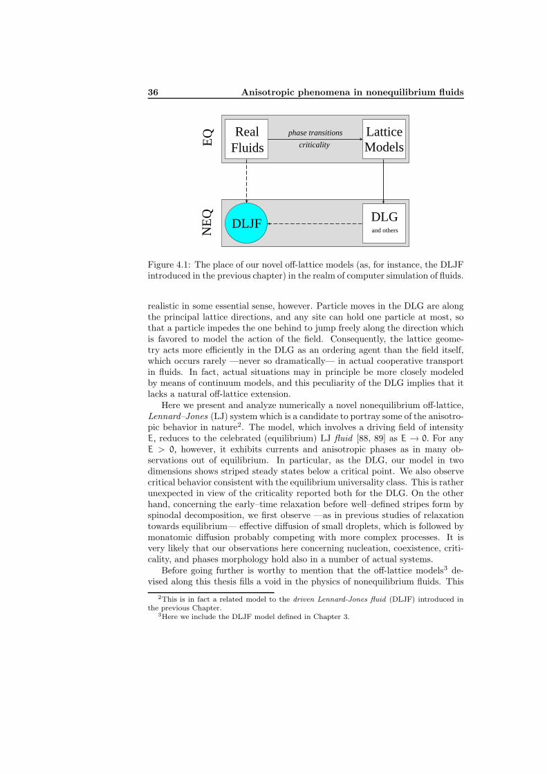
36 Anisotropic phenomena in nonequilibrium fluids
EQ
NE
Q
LatticeModels
RealFluids
DLGand others
DLJF
phase transitions
criticality
Figure 4.1: The place of our novel off-lattice models (as, for instance, the DLJFintroduced in the previous chapter) in the realm of computer simulation of fluids.
realistic in some essential sense, however. Particle moves in the DLG are alongthe principal lattice directions, and any site can hold one particle at most, sothat a particle impedes the one behind to jump freely along the direction whichis favored to model the action of the field. Consequently, the lattice geome-try acts more efficiently in the DLG as an ordering agent than the field itself,which occurs rarely —never so dramatically— in actual cooperative transportin fluids. In fact, actual situations may in principle be more closely modeledby means of continuum models, and this peculiarity of the DLG implies that itlacks a natural off-lattice extension.
Here we present and analyze numerically a novel nonequilibrium off-lattice,Lennard–Jones (LJ) system which is a candidate to portray some of the anisotro-pic behavior in nature2. The model, which involves a driving field of intensityE, reduces to the celebrated (equilibrium) LJ fluid [88, 89] as E → 0. For anyE > 0, however, it exhibits currents and anisotropic phases as in many ob-servations out of equilibrium. In particular, as the DLG, our model in twodimensions shows striped steady states below a critical point. We also observecritical behavior consistent with the equilibrium universality class. This is ratherunexpected in view of the criticality reported both for the DLG. On the otherhand, concerning the early–time relaxation before well–defined stripes form byspinodal decomposition, we first observe —as in previous studies of relaxationtowards equilibrium— effective diffusion of small droplets, which is followed bymonatomic diffusion probably competing with more complex processes. It isvery likely that our observations here concerning nucleation, coexistence, criti-cality, and phases morphology hold also in a number of actual systems.
Before going further is worthy to mention that the off-lattice models3 de-vised along this thesis fills a void in the physics of nonequilibrium fluids. This
2This is in fact a related model to the driven Lennard-Jones fluid (DLJF) introduced inthe previous Chapter.
3Here we include the DLJF model defined in Chapter 3.
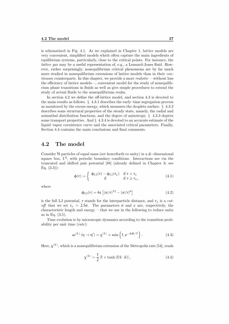
4.2 The model 37
is schematized in Fig. 4.1. As we explained in Chapter 1, lattice models arevery convenient, simplified models which often capture the main ingredients ofequilibrium systems, particularly, close to the critical points. For instance, thelattice gas may be a useful representation of, e.g., a Lennard-Jones fluid. How-ever, rather surprisingly, nonequilibrium critical phenomena are by far muchmore studied in nonequilibrium extensions of lattice models than in their con-tinuum counterparts. In this chapter, we provide a more realistic —without lossthe efficiency of lattice models—, convenient model for the study of nonequilib-rium phase transitions in fluids as well as give simple procedures to extend thestudy of actual fluids to the nonequilibrium realm.
In section 4.2 we define the off-lattice model, and section 4.3 is devoted tothe main results as follows. § 4.3.1 describes the early–time segregation processas monitored by the excess energy, which measures the droplets surface. § 4.3.2describes some structural properties of the steady state, namely, the radial andazimuthal distribution functions, and the degree of anisotropy. § 4.3.3 depictssome transport properties. And § 4.3.4 is devoted to an accurate estimate of theliquid–vapor coexistence curve and the associated critical parameters. Finally,Section 4.4 contains the main conclusions and final comments.
4.2 The model
Consider N particles of equal mass (set henceforth to unity) in a d−dimensionalsquare box, Ld, with periodic boundary conditions. Interactions are via thetruncated and shifted pair potential [88] (already defined in Chapter 3; seeEq. (3.3)):
φ(r) =
φLJ(r) − φLJ(rc) if r < rc
0 if r > rc,(4.1)
where
φLJ(r) = 4ε[
(σ/r)12 − (σ/r)6]
(4.2)
is the full LJ potential, r stands for the interparticle distance, and rc is a cut-off that we set rc = 2.5σ. The parameters σ and ε are, respectively, thecharacteristic length and energy —that we use in the following to reduce unitsas in Eq. (3.5).
Time evolution is by microscopic dynamics according to the transition prob-ability per unit time (rate):
ω(E) (η → η′) = χ(E) × min1, e−∆Φ/T
. (4.3)
Here, χ(E), which is a nonequilibrium extension of the Metropolis rate [54], reads
χ(E) =1
2[1 + tanh (Ex · δ)] , (4.4)
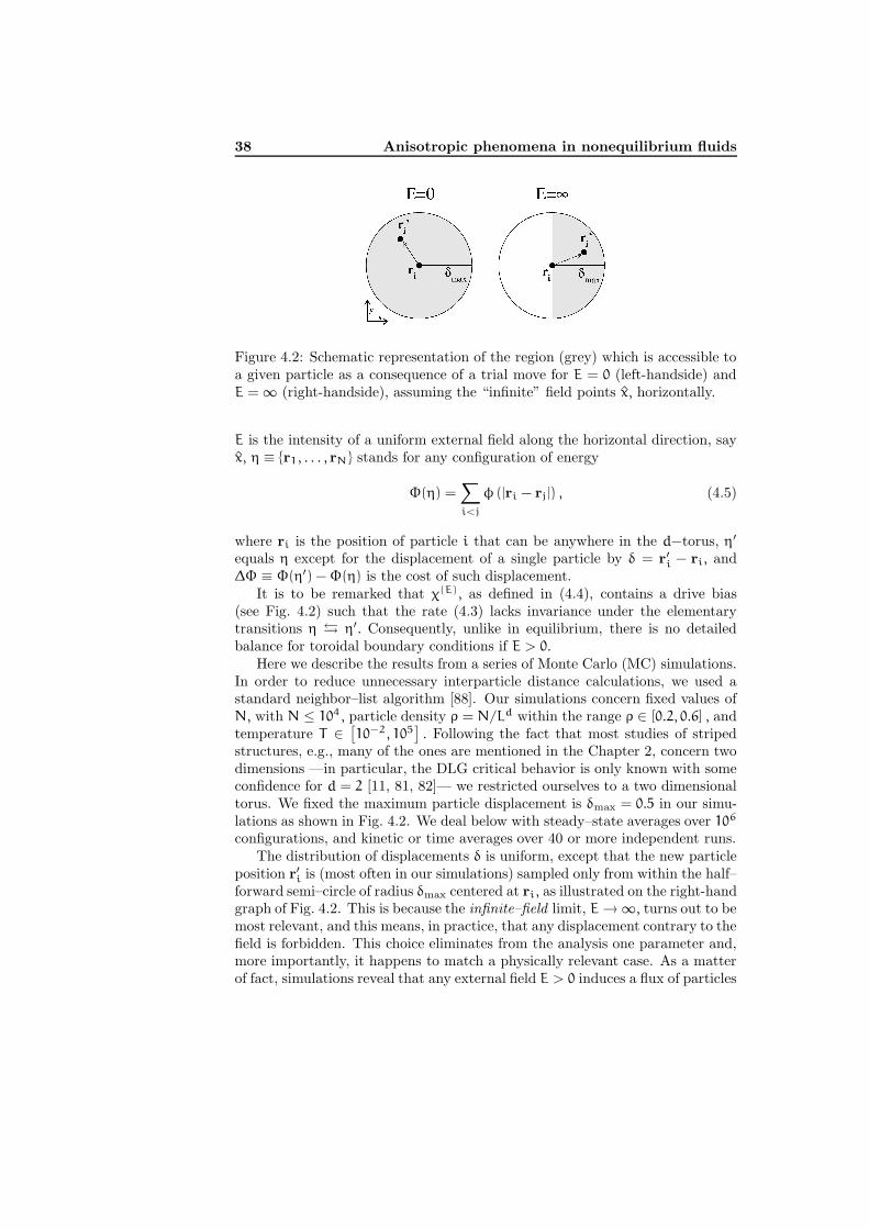
38 Anisotropic phenomena in nonequilibrium fluids
Figure 4.2: Schematic representation of the region (grey) which is accessible toa given particle as a consequence of a trial move for E = 0 (left-handside) andE = ∞ (right-handside), assuming the “infinite” field points x, horizontally.
E is the intensity of a uniform external field along the horizontal direction, sayx, η ≡ r1, . . . , rN stands for any configuration of energy
Φ(η) =∑
i<j
φ (|ri − rj|) , (4.5)
where ri is the position of particle i that can be anywhere in the d−torus, η′
equals η except for the displacement of a single particle by δ = r′i − ri, and∆Φ ≡ Φ(η′) − Φ(η) is the cost of such displacement.
It is to be remarked that χ(E), as defined in (4.4), contains a drive bias(see Fig. 4.2) such that the rate (4.3) lacks invariance under the elementarytransitions η η′. Consequently, unlike in equilibrium, there is no detailedbalance for toroidal boundary conditions if E > 0.
Here we describe the results from a series of Monte Carlo (MC) simulations.In order to reduce unnecessary interparticle distance calculations, we used astandard neighbor–list algorithm [88]. Our simulations concern fixed values ofN, with N ≤ 104, particle density ρ = N/Ld within the range ρ ∈ [0.2, 0.6] , andtemperature T ∈
[
10−2, 105]
. Following the fact that most studies of stripedstructures, e.g., many of the ones are mentioned in the Chapter 2, concern twodimensions —in particular, the DLG critical behavior is only known with someconfidence for d = 2 [11, 81, 82]— we restricted ourselves to a two dimensionaltorus. We fixed the maximum particle displacement is δmax = 0.5 in our simu-lations as shown in Fig. 4.2. We deal below with steady–state averages over 106
configurations, and kinetic or time averages over 40 or more independent runs.The distribution of displacements δ is uniform, except that the new particle
position r′i is (most often in our simulations) sampled only from within the half–forward semi–circle of radius δmax centered at ri, as illustrated on the right-handgraph of Fig. 4.2. This is because the infinite–field limit, E → ∞, turns out to bemost relevant, and this means, in practice, that any displacement contrary to thefield is forbidden. This choice eliminates from the analysis one parameter and,more importantly, it happens to match a physically relevant case. As a matterof fact, simulations reveal that any external field E > 0 induces a flux of particles
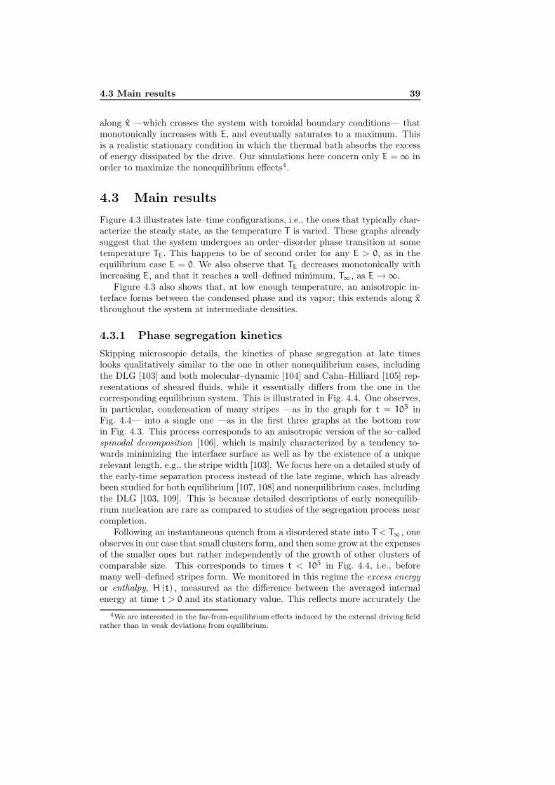
4.3 Main results 39
along x —which crosses the system with toroidal boundary conditions— thatmonotonically increases with E, and eventually saturates to a maximum. Thisis a realistic stationary condition in which the thermal bath absorbs the excessof energy dissipated by the drive. Our simulations here concern only E = ∞ inorder to maximize the nonequilibrium effects4.
4.3 Main results
Figure 4.3 illustrates late–time configurations, i.e., the ones that typically char-acterize the steady state, as the temperature T is varied. These graphs alreadysuggest that the system undergoes an order–disorder phase transition at sometemperature TE. This happens to be of second order for any E > 0, as in theequilibrium case E = 0. We also observe that TE decreases monotonically withincreasing E, and that it reaches a well–defined minimum, T∞, as E → ∞.
Figure 4.3 also shows that, at low enough temperature, an anisotropic in-terface forms between the condensed phase and its vapor; this extends along x
throughout the system at intermediate densities.
4.3.1 Phase segregation kinetics
Skipping microscopic details, the kinetics of phase segregation at late timeslooks qualitatively similar to the one in other nonequilibrium cases, includingthe DLG [103] and both molecular–dynamic [104] and Cahn–Hilliard [105] rep-resentations of sheared fluids, while it essentially differs from the one in thecorresponding equilibrium system. This is illustrated in Fig. 4.4. One observes,in particular, condensation of many stripes —as in the graph for t = 105 inFig. 4.4— into a single one —as in the first three graphs at the bottom rowin Fig. 4.3. This process corresponds to an anisotropic version of the so–calledspinodal decomposition [106], which is mainly characterized by a tendency to-wards minimizing the interface surface as well as by the existence of a uniquerelevant length, e.g., the stripe width [103]. We focus here on a detailed study ofthe early-time separation process instead of the late regime, which has alreadybeen studied for both equilibrium [107, 108] and nonequilibrium cases, includingthe DLG [103, 109]. This is because detailed descriptions of early nonequilib-rium nucleation are rare as compared to studies of the segregation process nearcompletion.
Following an instantaneous quench from a disordered state into T < T∞, oneobserves in our case that small clusters form, and then some grow at the expensesof the smaller ones but rather independently of the growth of other clusters ofcomparable size. This corresponds to times t < 105 in Fig. 4.4, i.e., beforemany well–defined stripes form. We monitored in this regime the excess energyor enthalpy, H (t) , measured as the difference between the averaged internalenergy at time t > 0 and its stationary value. This reflects more accurately the
4We are interested in the far-from-equilibrium effects induced by the external driving fieldrather than in weak deviations from equilibrium.
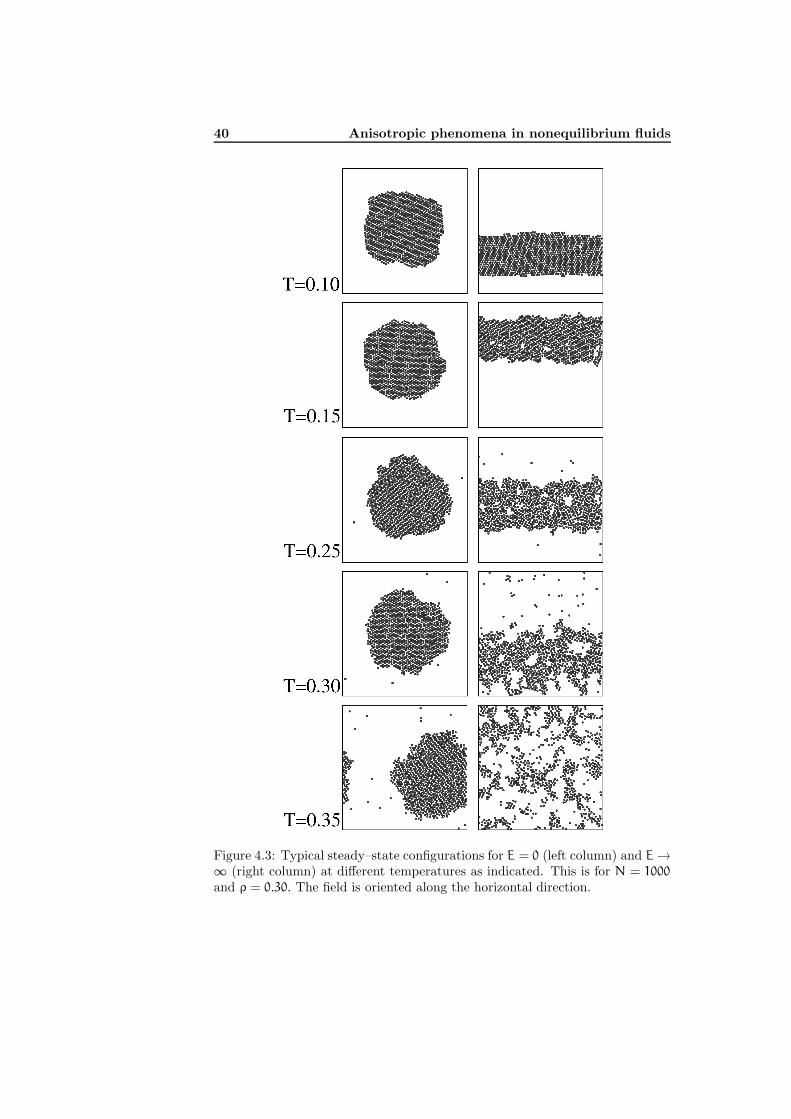
40 Anisotropic phenomena in nonequilibrium fluids
Figure 4.3: Typical steady–state configurations for E = 0 (left column) and E →∞ (right column) at different temperatures as indicated. This is for N = 1000
and ρ = 0.30. The field is oriented along the horizontal direction.

4.3 Main results 41
Figure 4.4: Typical configurations for E = 0 (top row) and E → ∞ (bottom row)as time proceeds during relaxation from a disordered state (as for T → ∞) att = 0. The time here is proportional to the MC steps (MCS) as indicated. Thisis for N = 7500, ρ = 0.35, and T = 0.275, below the corresponding transitiontemperature.

42 Anisotropic phenomena in nonequilibrium fluids
103
104
105
106
t0.1
0.2
0.3
0.4
h
101
102
103
1
t-0.6
t-0.5
t-0.4
t-0.3
t-0.165
(a)
(b)
(c)
Figure 4.5: Time evolution of the enthalpy per particle for N = 7500, ρ = 0.35
and, from top to bottom, T = 0.200, 0.225, 0.250, and 0.275. Straight lines area guide to the eye; the slope of each line is indicated. The inset shows the detailat early times. (For clarity of presentation, the main graph includes a rescalingof the time corresponding to the data for T = 0.250, 0.225 and 0.200 by factors2, 3 and 3, respectively.)
growth of the condensed droplets than its size or radius, which are difficult tobe estimated during the early stages [110, 111]. In addition to its theoreticalimportance, the excess of energy may be relevant for experimentalists. This isbecause H (t) may be determined in microcalorimetric experiments [112].
The time development of the enthalpy density h (t) = H (t) /N is depictedin Fig. 4.5. This reveals some well–defined regimes at early times.
The first regime, (a) in the inset of Fig. 4.5, follows a power law t−θ with θ ≈1/6 —which corresponds to the line shown in the graph— independently of thetemperature investigated. This is the behavior predicted by the Smoluchowskicoagulation or effective cluster diffusion [99]. The same behavior was observed incomputer simulations for E = 0 and also reported to hold in actual experimentson binary mixtures [110, 112]. Surprisingly, this suggests the early dominanceof a rather stochastic mechanism, in which the small clusters rapidly nucleate,which is practically independent of the field, i.e., it is not affected in practice bythe drive. It is also noticeable that, in contrast with simulations on lattice gasesin which this regime is rather noisy, a slope t−1/6 appears clearly in Fig. 4.5.The indication of some temperature dependence in equilibrium [111], which isnot evident here, might correspond to the distinction between deep and shallowquenches made in Ref. [110] that we have not investigated out of equilibrium.
At later times, there is a second regime, (b) in Fig. 4.5, in which theanisotropic clusters merge into filaments and, finally, stripes. We observe in thisregime that θ varies between 0.3 and 0.6 with increasing T . Ostwald ripening[113], consisting of monomers diffusion, predicts θ = 1/3 for fluids at thermal

4.3 Main results 43
Figure 4.6: Details of the structure in the low−T, solid phase as obtained byzooming into configurations such as the ones in Fig. 4.3. This is for T = 0.05,
0.12, and 0.25, from left to right, respectively.
equilibrium. The situation here in our nonequilibrium is more complicate: it islikely that regime (b) describes a crossover from a situation which is dominatedby monomers at low enough temperature to the emergence of other mechanisms[108, 114] which might be competing as T is increased.
Finally, one observes a regime, (c) in Fig. 4.5, which corresponds to thebeginning of spinodal decomposition.
4.3.2 Structure of the steady state
Concerning the local structure in the stationary regime, for any E > 0, theanisotropic condensate changes from a solidlike hexagonal packing of particlesat low temperature (e.g., T = 0.10 in Fig. 4.3), to a polycrystalline or perhapsglass–like structure with domains which show a varied morphology at, e.g.,T = 0.12. The latter phase further transforms, with increasing temperature,into a fluid–like structure at, e.g., T = 0.30 and, finally, into a disordered,gaseous state.
More specifically, the typical situation we observe at low temperature isillustrated in Fig. 4.6. At sufficiently low temperature, T = 0.05 in the example,the whole condensed phase orders according to a perfect hexagon with one ofits main directions along the field direction x. This is observed in approximately90% of the configurations that we generated at T = 0.05, while all the hexagonaxes are slanted with respect to x in the other 10% cases. As the system isheated up, the stripe looks still solid at T = 0.12 but, as illustrated by thesecond graph in Fig. 4.6, one observes in this case several coexisting hexagonaldomains with different orientations. The separation between domains is byline defects and/or vacancies. Interesting enough, as it will be shown later on,both the system energy and the particle current are practically independent oftemperature up to, say T = 0.12. The hexagonal ordering finally disappears inthe third graph of Fig. 4.6, which is for T = 0.25; this case corresponds to afluid phase according to the criterion below.

44 Anisotropic phenomena in nonequilibrium fluids
0.25 0.3 0.35T
0
0.5
1
1.5
2
2.5
3
D -π/2 -π/4 0 π/4 π/2θ
0.5
1
1.5
2
AD
0 1 2 3 43r
0
1
2
3
4
5
RD
Figure 4.7: Data from simulations for N = 7000 and ρ = 0.35. The main graphshows the degree of anisotropy, as defined in the main text, versus temperature.The vertical dotted line denotes the transition temperature. The lower (upper)inset shows the radial (azimuthal) distribution at T = 0.20, full line, and T =
0.30, dashed line.
A close look to the structure is provided by the radial distribution (RD),
g (r) = ρ−2
⟨
∑
i<j
δ (ri − rj)
⟩
, (4.6)
i.e., the probability of finding a pair of particles a distance r apart, relative tothe case of a random spatial distribution at same density. This is shown inthe lower inset of Fig. 4.7. At fixed T, the driven fluid is less structured thanits equilibrium counterpart, suggesting that the field favors disorder. This isalready evident in Fig. 4.3, and it also follows from the fact that the criticaltemperature decreases with increasing E.
Further information on the essential anisotropy of the problem is beared bythe azimuthal distribution (AD), which accounts for the longe range ordering.This is defined
α(θ) = N−2
⟨
∑
i<j
δ (θ − θij)
⟩
, (4.7)
where θij ∈ [0, 2π) is the angle between the line connecting particles i and j
and the field direction x. Except at equilibrium, where this is uniform, the ADis π/2−periodic with maxima at kπ and minima at kπ/2, where k is an integer.This means that the field favors long-range longitudinal ordering instead oforder along other directions. This is consistent with the observations in whichthe orientations of the hexagons in the solidlike phase are parallel to the fielddirection. The AD is depicted in the upper inset of Fig. 4.7.
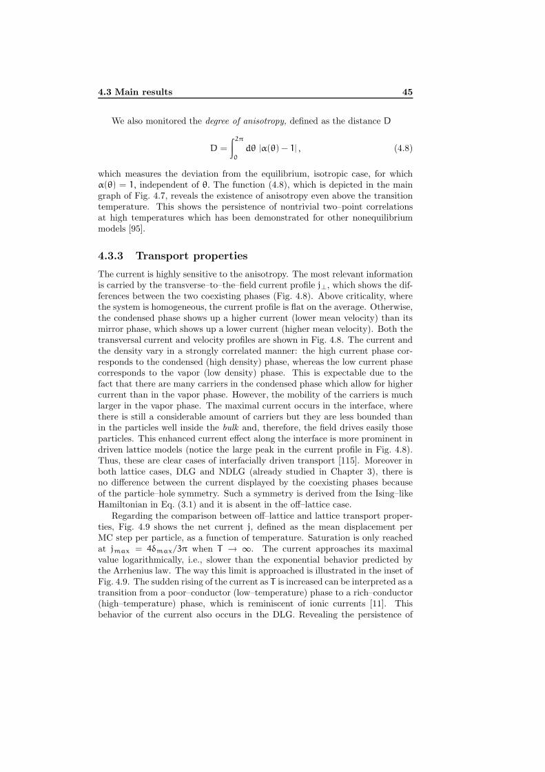
4.3 Main results 45
We also monitored the degree of anisotropy, defined as the distance D
D =
∫2π
0
dθ |α(θ) − 1| , (4.8)
which measures the deviation from the equilibrium, isotropic case, for whichα(θ) = 1, independent of θ. The function (4.8), which is depicted in the maingraph of Fig. 4.7, reveals the existence of anisotropy even above the transitiontemperature. This shows the persistence of nontrivial two–point correlationsat high temperatures which has been demonstrated for other nonequilibriummodels [95].
4.3.3 Transport properties
The current is highly sensitive to the anisotropy. The most relevant informationis carried by the transverse–to–the–field current profile j⊥, which shows the dif-ferences between the two coexisting phases (Fig. 4.8). Above criticality, wherethe system is homogeneous, the current profile is flat on the average. Otherwise,the condensed phase shows up a higher current (lower mean velocity) than itsmirror phase, which shows up a lower current (higher mean velocity). Both thetransversal current and velocity profiles are shown in Fig. 4.8. The current andthe density vary in a strongly correlated manner: the high current phase cor-responds to the condensed (high density) phase, whereas the low current phasecorresponds to the vapor (low density) phase. This is expectable due to thefact that there are many carriers in the condensed phase which allow for highercurrent than in the vapor phase. However, the mobility of the carriers is muchlarger in the vapor phase. The maximal current occurs in the interface, wherethere is still a considerable amount of carriers but they are less bounded thanin the particles well inside the bulk and, therefore, the field drives easily thoseparticles. This enhanced current effect along the interface is more prominent indriven lattice models (notice the large peak in the current profile in Fig. 4.8).Thus, these are clear cases of interfacially driven transport [115]. Moreover inboth lattice cases, DLG and NDLG (already studied in Chapter 3), there isno difference between the current displayed by the coexisting phases becauseof the particle–hole symmetry. Such a symmetry is derived from the Ising–likeHamiltonian in Eq. (3.1) and it is absent in the off–lattice case.
Regarding the comparison between off–lattice and lattice transport proper-ties, Fig. 4.9 shows the net current j, defined as the mean displacement perMC step per particle, as a function of temperature. Saturation is only reachedat jmax = 4δmax/3π when T → ∞. The current approaches its maximalvalue logarithmically, i.e., slower than the exponential behavior predicted bythe Arrhenius law. The way this limit is approached is illustrated in the inset ofFig. 4.9. The sudden rising of the current as T is increased can be interpreted as atransition from a poor–conductor (low–temperature) phase to a rich–conductor(high–temperature) phase, which is reminiscent of ionic currents [11]. Thisbehavior of the current also occurs in the DLG. Revealing the persistence of
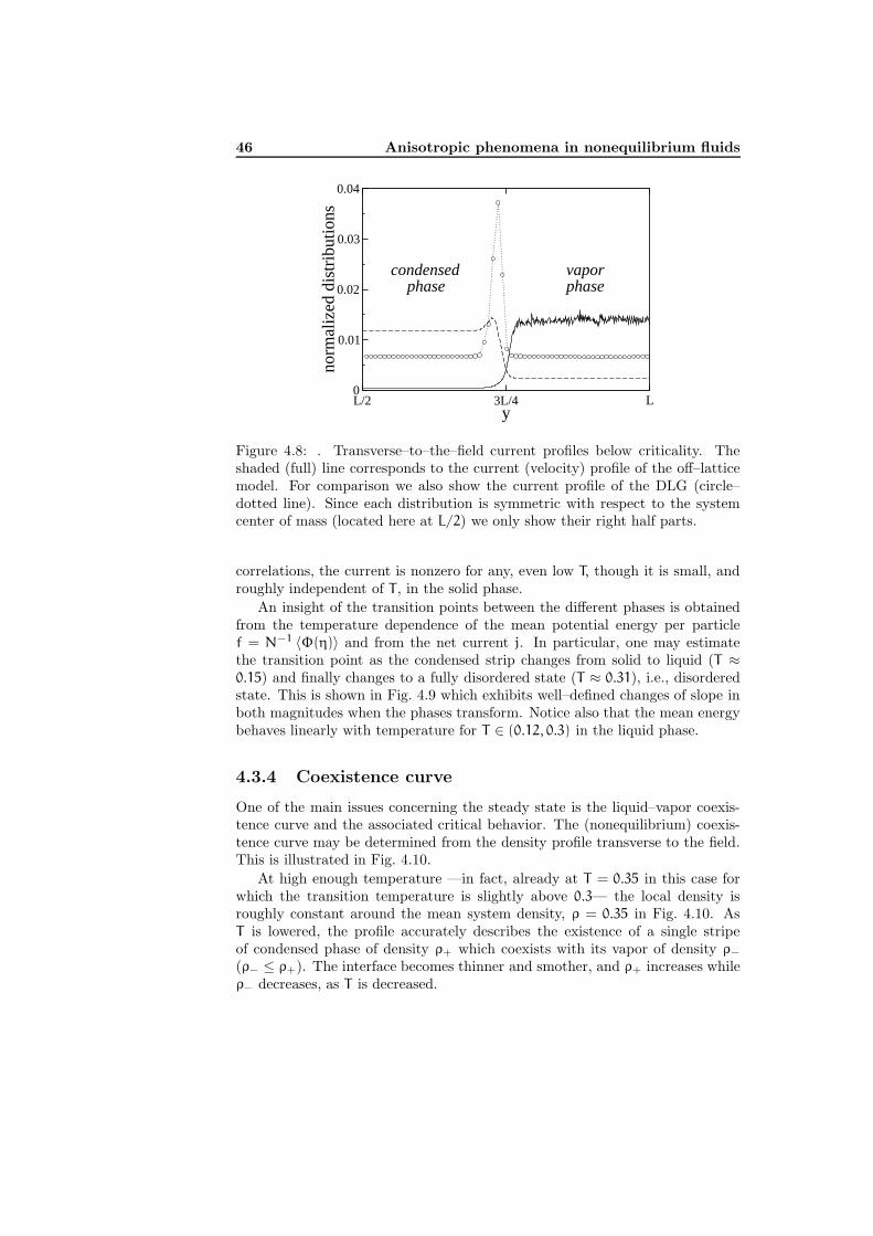
46 Anisotropic phenomena in nonequilibrium fluids
L/2 3L/4 Ly
0
0.01
0.02
0.03
0.04
norm
aliz
ed d
istr
ibut
ions
condensed phase
vaporphase
Figure 4.8: . Transverse–to–the–field current profiles below criticality. Theshaded (full) line corresponds to the current (velocity) profile of the off–latticemodel. For comparison we also show the current profile of the DLG (circle–dotted line). Since each distribution is symmetric with respect to the systemcenter of mass (located here at L/2) we only show their right half parts.
correlations, the current is nonzero for any, even low T, though it is small, androughly independent of T , in the solid phase.
An insight of the transition points between the different phases is obtainedfrom the temperature dependence of the mean potential energy per particlef = N−1 〈Φ(η)〉 and from the net current j. In particular, one may estimatethe transition point as the condensed strip changes from solid to liquid (T ≈0.15) and finally changes to a fully disordered state (T ≈ 0.31), i.e., disorderedstate. This is shown in Fig. 4.9 which exhibits well–defined changes of slope inboth magnitudes when the phases transform. Notice also that the mean energybehaves linearly with temperature for T ∈ (0.12, 0.3) in the liquid phase.
4.3.4 Coexistence curve
One of the main issues concerning the steady state is the liquid–vapor coexis-tence curve and the associated critical behavior. The (nonequilibrium) coexis-tence curve may be determined from the density profile transverse to the field.This is illustrated in Fig. 4.10.
At high enough temperature —in fact, already at T = 0.35 in this case forwhich the transition temperature is slightly above 0.3— the local density isroughly constant around the mean system density, ρ = 0.35 in Fig. 4.10. AsT is lowered, the profile accurately describes the existence of a single stripeof condensed phase of density ρ+ which coexists with its vapor of density ρ−
(ρ− ≤ ρ+). The interface becomes thinner and smother, and ρ+ increases whileρ− decreases, as T is decreased.

4.3 Main results 47
0
0.1
0.2
0.3
j/jmax
0 0.1 0.2 0.3 0.4 0.5T
-3
-2.5
-2
-1.5
-1
f100
102
104
T0
0.2
0.4
0.6
0.8
1
j/jmax
Figure 4.9: Temperature dependence of the mean energy (squares; the scale is onthe right axis) and normalized net current (circles; scale at the left) for N = 5000
and ρ = 0.30 under “infinite” field. The inset shows the T−dependence of thecurrent over a wider range.
0 L/2 LL/4 3L/4y
0
0.2
0.4
0.6
0.8
ρ ⊥
T=0.200
T=0.300
T=0.250
T=0.350
ρ+
ρ− ρ−
Figure 4.10: Density profiles transverse to the field for N = 7000, ρ = 0.35, anddifferent temperature, as indicated. The coexisting densities, ρ±, are indicated.

48 Anisotropic phenomena in nonequilibrium fluids
Table 4.1: Critical parametersρ∞ T∞ β
0.321(5) 0.314(1) 0.10(8)
As in equilibrium, one may use ρ+ − ρ− as an order parameter. The resultof plotting ρ+ and ρ− at each temperature results in the non-symmetric liquid-vapor coexistence curve shown in Fig. 4.11. The same result follows from thecurrent, which in fact varies strongly correlated with the local density. Noticethat the accuracy of our estimate of ρ± is favored by the existence of a linearinterface, which enable us to get closer to the critical point than in equilibrium.Lacking a thermodynamic theory for “phase transitions” in nonequilibrium liq-uids, other approaches have to be considered in order to estimate the criticalparameters.
Consider to the rectilinear diameter law
1
2(ρ+ + ρ−) = ρ∞ + b0(T∞ − T), (4.9)
which is a empirical fit [4] extensively used for fluids in equilibrium. Here ρ∞
and T∞ denotes the critical density and the critical temperature, respectively.This, in principle, has no justification out of equilibrium. However, we foundthat our MC data nicely fit the diameters equation. We use this fact togetherwith a universal scaling law5
ρ+ − ρ− = a0(T∞ − T)β, (4.10)
to accurately estimate the critical parameters. The simulation data in Fig. 4.11then yields the values in Table 4.1, which are confirmed by the familiar log–logplots. Compared to the equilibrium critical temperature reported by Smit andFrenkel [89], one has that T0/T∞ ≈ 1.46, i.e., the change is opposite to the onefor the DLG [11]. This confirms the observation above that the field acts in thenonequilibrium LJ system favoring disorder.
The fact that the order–parameter critical exponent is relatively small mayalready be guessed by noticing the extremely flat coexistence curve in Fig. 4.11.This is similar to the corresponding curve for the equilibrium two–dimensionalLJ fluids [89, 117, 118], and it is fully consistent with the equilibrium Onsagervalue, β = 1/8. We therefore believe that our model belongs to the Ising uni-versality class. In any case, although the error bar is large, one may discardwith confidence both the DLG value β ≈ 1/3 as well as the mean field valueβ = 1/2 —both cases would produce a hump visible to the naked eye in a plotsuch as the one in Fig. 4.11. One may argue that this result is counterintuitive,as our model apparently has the short–range interactions and symmetries thatare believed to characterize the DLG. Further understanding for this differencewill perhaps come from the statistical field theory.
5The first term of a Wegner-type expansion [116].
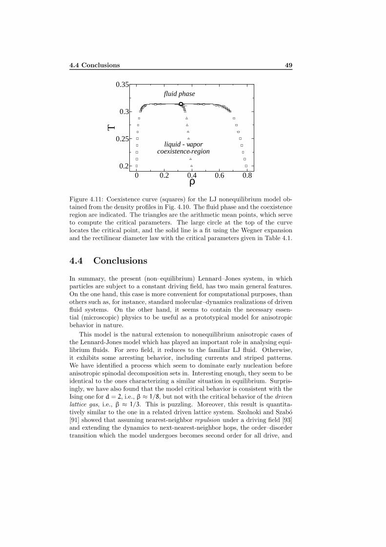
4.4 Conclusions 49
0 0.2 0.4 0.6 0.8ρ0.2
0.25
0.3
0.35
T
fluid phase
liquid - vapor coexistence region
Figure 4.11: Coexistence curve (squares) for the LJ nonequilibrium model ob-tained from the density profiles in Fig. 4.10. The fluid phase and the coexistenceregion are indicated. The triangles are the arithmetic mean points, which serveto compute the critical parameters. The large circle at the top of the curvelocates the critical point, and the solid line is a fit using the Wegner expansionand the rectilinear diameter law with the critical parameters given in Table 4.1.
4.4 Conclusions
In summary, the present (non–equilibrium) Lennard–Jones system, in whichparticles are subject to a constant driving field, has two main general features.On the one hand, this case is more convenient for computational purposes, thanothers such as, for instance, standard molecular–dynamics realizations of drivenfluid systems. On the other hand, it seems to contain the necessary essen-tial (microscopic) physics to be useful as a prototypical model for anisotropicbehavior in nature.
This model is the natural extension to nonequilibrium anisotropic cases ofthe Lennard-Jones model which has played an important role in analysing equi-librium fluids. For zero field, it reduces to the familiar LJ fluid. Otherwise,it exhibits some arresting behavior, including currents and striped patterns.We have identified a process which seem to dominate early nucleation beforeanisotropic spinodal decomposition sets in. Interesting enough, they seem to beidentical to the ones characterizing a similar situation in equilibrium. Surpris-ingly, we have also found that the model critical behavior is consistent with theIsing one for d = 2, i.e., β ≈ 1/8, but not with the critical behavior of the drivenlattice gas, i.e., β ≈ 1/3. This is puzzling. Moreover, this result is quantita-tively similar to the one in a related driven lattice system. Szolnoki and Szabo[91] showed that assuming nearest-neighbor repulsion under a driving field [93]and extending the dynamics to next-nearest-neighbor hops, the order–disordertransition which the model undergoes becomes second order for all drive, and
50 Anisotropic phenomena in nonequilibrium fluids
belongs to the Ising universality class. Furthermore, it is straightforward to seethat if one allows particles’ spatial coordinates to vary continuously then themodel reduces to a hard-disks gas under a driving field, and the second orderphase transition vanishes. The transition becomes similar to the melting tran-sition for systems in equilibrium, which is described by the KTHNY scenario[119]. The fact that in both nonequilibrium diffusive models —which share sim-ilar dynamics— the critical behavior is consistent with Ising is rather surprising.For instance, using bare arguments of statistical field theory, symmetries seemto bring our system closer to the nonequilibrium lattice model (the DLG) thanto the corresponding equilibrium case (the LJ fluid).
Therefore, a principal conclusion is that —regarding the modeling of complexsystems— spatial discretization may change significantly not only morphologi-cal properties, but also critical properties. This is in contrast with the conceptof universality in equilibrium systems, where critical properties are indepen-dent of dynamic details. The main reason for this disagreement might be theparticle–hole symmetry violation in the driven Lennard–Jones fluid. However,to determine exactly this statement will require further study.
In any case, the additional freedom of the present, off–lattice system, whichin particular implies that the particle–hole symmetry which occurs in latticemodels is violated —which induces the coexistence-curve asymmetry in Fig. 4.11in accordance with actual systems— are likely to matter more than suggested bysome naive intuition. Indeed, the question of what are the most relevant ingre-dients and symmetries which determine unambiguously the universal propertiesin driven diffusive fluids is still open. Nevertheless, the above important dif-ference between the lattice and the off–lattice cases results most interesting asan unquestionable nonequilibrium effect; as it is well known, such microscopicdetail is irrelevant to universality concerning equilibrium critical phenomena.
Future investigations should address the development of a field theoreticaldescription which shed light on the critical behavior of these models. Off–latticemodels pose a new challenge for any available Langevin-type approach in whichto test their viability. In principle, the anisotropic diffusive system approachdescribed in the previous Chapter seems to be more appropriate because of itallows for considering the microscopic dynamical details. In fact, it is expectedthat a careful analysis in the derivation process from the master equation to thefinal Langevin equation should revail to identify the mechanisms that lead toIsing behavior.
Further study of the present nonequilibrium LJ system and its possible vari-ations is suggested. A principal issue to be investigated is the apparent factthat the full nonequilibrium situations of interest can be described by somerather straightforward extension of equilibrium theory. We here deal with someindications of this concerning early nucleation and properties of the coexistencecurve. No doubt it would be interesting to compare more systematically thebehavior of models against the varied phenomenology which was already re-ported for anisotropic fluids. This should also help a better understanding ofnonequilibrium critical phenomena.

4.4 Conclusions 51
Finally, one of our main aims at proposing this model has been motivatefurther research, both experimental and theoretical: we try to motivate newexperiments on anisotropic decomposition besides theoretical work. In fact,our observations on the early-time separation process and structural propertiesare easily accessible by micro calorimetric and spectroscopy experiments, forinstance.
52 Anisotropic phenomena in nonequilibrium fluids

Part II
Driven Granular Gases


Chapter 5
Introduction
The second part of this thesis focuses on rapid granular flows, also referred asgranular gases [120, 121, 122, 123, 124]. They are granular systems fluidizedby the application of an external driving, e.g., by mechanical vibration [39, 44],shear [125], electrostatically [126], or others means [41, 127]. In these systems,collisions between particles are considered nearly instantaneous compared withthe mean free time. In fact, it is assumed (by definition) that the flow is gov-erned by binary collisions —as in molecular gases—, whereas three–body (ormore) collisions are neglected. Instead of moving in many–particle blocks, eachparticle moves freely and independently of even its nearest neighbors. Fur-thermore, granular gases exhibit many states and instabilities, e.g., convection[48, 49, 128], that characterize molecular gases. In spite of these similarities withclassical molecular fluids, there are significant differences between both whichmake granular gases strikingly different. The origin of differences lies, as notedin the general introduction (Chapter 1), in the inelastic character of collisionsbetween grains, and in the irrelevance of the thermal energy kBT .
One important coarse-grained (continuum) approach to modeling granulargases is hydrodynamics. Granular hydrodynamics has a great predictive powerand looks ideally suitable for a description of large–scale —long-wavelengthand long-time— patterns observed in rapid granular flows as, for instance, aplethora of clustering phenomena [43, 44, 129, 130], vortices [37, 131, 132], os-cillons [39, 133], and shocks [134]. This approach consists on a set of partialdifferential equations for the velocity v(r, t), temperature T(r, t) (average fluc-tuation kinetic energy), pressure p(r, t), and density (or number density n(r, t))ρ(r, t) fields. Hydrodynamic equations are analogous to the Navier Stokes equa-tions for molecular fluids, but include a sink term in the energy equation whichaccounts for dissipation in collisions. For two-dimensional granular fluids, these

56 Introduction
read
∂n
∂t+ ∇ (nv) = 0 mass conservation,
n
(
∂v
∂t+ (v · ∇)v
)
= ∇ · p + ng momentum conservation,
n
(
∂T
∂t+ (v · ∇) T
)
= −∇ · w + p : ∇v − I energy conservation.
(5.1)
Here, p is the stress tensor, w is the heat flux, I is the rate of energy loss bycollisions per unit area per unit time, and g is a external force acting on theparticles. Under some assumptions, more fundamental kinetic theory validatesthese equations and supplies constitutive relations1 [135, 136, 137]. However,the exact criteria for the validity of (granular) kinetic theory and Navier–Stokeshydrodynamics [135, 138, 139] is still lacking. This is because first–principlederivations of universally applicable continuum theory of granular gas is nota simple task, even in the dilute limit. Unfortunately, the drastic simplifica-tion, provided by the binary collisions assumption, is far from sufficient for aderivation of hydrodynamics, and additional hypothesis are needed. Assuminga hard-disks system, and that the random motion of even neighboring particlesare uncorrelated (molecular chaos assumption or stosszahlansatz ) allows forderivations from the Boltzmann or Chapman-Enskog kinetic equation, properlygeneralized to account for the inelasticity of the particle collisions. An importantadditional assumption, made in the process of the derivation of hydrodynamicsfrom the Chapman–Enskog equation, is scale separation [124]. Hydrodynamicsdemands (for inhomogeneous and/or unsteady) flows that the mean free pathof the particles is much less than any characteristic length scale, and the meanfree time between two consecutive collisions be much less than any characteris-tic time scale, aimed to be described hydrodynamically. All of these hypothesisare justified for moderate densities and for not too large inelasticity. Theseshould be verified, in every specific system, after the hydrodynamic problem issolved and the characteristic length and time scales determined. In such case,systematic derivations of the constitutive relations —the equation of state andtransport coefficients— of granular hydrodynamics from the Boltzmann or En-skog equation [140, 141, 142] use an expansion in the Knudsen number and, insome versions of theory, in inelasticity [140].
A finite inelasticity immediately brings complications [124]. Correlationsbetween particles, developing already at a moderate inelasticity, may invali-date the molecular chaos hypothesis [143]. The correlations become strongeras the inelasticity of the collisions increases. The normal stress difference anddeviations of the particle velocity distribution from the Maxwell distributionalso become important for inelastic collisions. As a result, the Navier-Stokesgranular hydrodynamics should not be expected to be quantitatively accuratebeyond the limit of small inelasticity. In any case, despite the severe limitationsintrinsic to it, the nearly elastic case is conceptually important, just because
1These are the explicit expressions of p, w, and I in terms of the basic fields n, T , and v.
57
hydrodynamics is supposed to give here a quantitatively accurate leading ordertheory. This is the regime (nearly elastic collisions) considered in the followingChapters 6 and 7.
A further set of difficulties for hydrodynamics arise at large densities. Inmono-disperse systems strong correlations appear, already for elastic hard spheres,at the disorder-order transition. As multiple thermodynamic phases may coex-ist there [144], a general continuum theory of hard sphere fluids, which hasyet to be developed, must include, in addition to the hydrodynamic fields, anorder-parameter field. Furthermore, even on a specified branch of the thermo-dynamic phase diagram, we do not have first–principle constitutive relations.Last but not least, kinetic theory of, for instance, a finite–density gas of elastichard spheres in two dimensions is plagued by non–existence of transport coeffi-cients because of the long-time tail in the velocity pair autocorrelation function[145, 146].
Another potentially important limitation of the validity of granular hydro-dynamics (or, rather, of any continuum approach to rapid granular flows) isdue to the noise caused by the discrete nature of particles. Noise is strongerhere than in classical molecular fluids simply because the number of particlesis much smaller. In addition, noise can be amplified at thresholds of hydro-dynamic instabilities as found, for example, in Rayleigh–Benard convection ofclassical fluids [147] or in granular gases [148]. A new challenge for theory is aquantitative account of this noise. A promising approach at small or moderatedensities is “Fluctuating Granular Hydrodynamics”: a Langevin–type theorythat takes into account the discrete particle noise by adding a delta–correlated(gaussian) noise terms in the momentum and energy equations, in the spiritof the Fluctuating Hydrodynamics by Landau and Lifshitz [149, 150]. At highdensities, however, such a theory is again beyond reach.
An alternative approach to granular flows, besides experiments, are simula-tions. Computer simulations have a valuable role in providing essentially exactresults for certain problems which would otherwise be intractable. In addition,simulations help us to obtain the intuition we need in order to understand thecomplex behavior exhibited by granular material. Here (Chapters 6 and 7), wetest the predictions from the hydrodynamic equations by comparing with Molec-ular Dynamics simulations [51, 88, 151]. Molecular Dynamics is a technique forcomputing the steady state and transport properties of a many–body system.This is in many respects very similar to real experiments. The general idea issimple: integrate numerically the microscopic equations of motion (Newton’sequations2) simultaneously for all particles (1 ≤ i ≤ N)
mi
d2ri
dt2= Fi(r1, · · · , rN,v1, · · · ,vN) (5.2)
This type of Molecular Dynamics is called force–based. However, there are sys-tems in which this scheme is very inefficient (although, of course, still applicable)
2Typically, because of the macroscopic size of grains, quantum effects can be discardedwith confidence.
58 Introduction
[51]. In systems where most of the time each of particles propagates along aballistic trajectory, the typical duration of a collision is much shorter than themean time between successive collisions of a particle, i.e., binary collisions canbe assumed. This is, in fact, what occurs in rapid granular flows. In such acase, if the post–collisional velocities are obtained from the pre–collisional ve-locities a event–driven Molecular Dynamics simulation can be set up3. As aresult, event–driven algorithms are much more efficient, in the sense of simu-lation speed, than force–based algorithms (integrating directly Eq. 5.2). Wewill employ event-driven molecular dynamic simulations to test the validity ofhydrodynamic prediction in the following chapters.
A standard prototypical model for driven granular gases, employed in manytheories and simulations, as well as in experiments, is that of a monodispersecollection of uniform frictionless hard spheres (hard disks in two–dimensions)whose collisions are characterized by constant normal restitution coefficient µ⊥4.Usually, this model is employed to study dense or diluted flows, with or withoutgravity, and with or without a interstitial fluid. Here the tangential degrees offreedom are neglected, i.e., µ‖ = 1, and only the normal restitution coefficientµ⊥ appears. However, it is worth mentioning that these two assumptions areill-suited (see a nice discussion in [51]). This simplification is owed exclusivelyto the huge theoretical complication which comes along with the incorporationof the correct (velocity dependent) tangential restitution coefficient. More com-plex models may involve nonspherical particles, in general, irregularly shapedparticles, and are also polydisperse. In addition, except for astrophysical stud-ies [122] or experiments performed in vacuum [39] the grains are embedded inan ambient fluid. Nonetheless, the effect of a interstitial fluid, as air or wa-ter, can be sometimes neglected in determining many properties of the system[120]. This is particularly true when grain–grain interactions are stronger thanfluid or grain–fluid interactions. But as the level of detail increases so does thecomputational effort. In spite of its shortcomings as a practical tool, the hard–spheres prototype enables the elucidation of many essential features which arethe responsible for the observed macroscopic behavior.
Regarding the mechanism which drives the particles, in Chapters 6 and 7 weconsider rapidly vibrating boundaries. We will assume that the characteristicfrequency of vibration of the wall is much larger than the collision rate of thegrains. This guarantees the absence of correlations between successive collisionsof particles with the vibrating wall. In addition, it will be assumed that theamplitude of the vibration is much smaller than the mean free path of the par-ticles, so collective motions in the system are avoided. Therefore, the vibratedwall can be represented as a hydrodynamic heat flux, i.e., as a “thermal” wall.From a computational point of view, the thermal wall is implemented as follows:
3There are previous works in which event–driven algorithms has been even applied to densegranular systems [130].
4The restitution coefficient typically depends weakly on the velocity, but using a constantsimplifies the theoretical derivations greatly [51].
59
whenever a particle collides with the wall, it forgets its velocity and chooses anew one from a Maxwell distribution according to a certain, previously pre-scribed temperature T . It is important to notice that in order to avoid that thegas approaches the incorrect final temperature, the random normal velocitieshave to be chosen according to the probability distribution
N(vn) =m
Tvnexp
[
−mv2
n
2T
]
, (5.3)
and the tangential velocities have to be determined from
N(vt) =
√
m
2πTexp
[
−mv2
t
2T
]
. (5.4)
See e.g. Ref. [51], pages 173-177, for detail.
The first simulation of a system of particles colliding ineslatically and drivenby a side themal wall was considered, in one dimension, by Du, Li, and Kadanoff[152]. For typical initial conditions, the system in Ref. [152] evolves to a statewhere the particles are separated into two groups. Almost all particles form alow–temperature cluster in a small region, while a few remaining particles movewith high velocities. Clearly, this steady state cannot be described by granularhydrodynamics. The results in Ref. [152] brought into question the validity ofgranular hydrodynamics in general. Nevertheless, some results [153, 154] haveshowed that this “anomaly” seems to vanish in higher dimensions (our studiesdeveloped in Chapters 6 and 7 concern two-dimensional systems). Therefore,the validity of hydrodynamics merits further studies.

60 Introduction
Chapter 6
Phase separation of a
driven granular gas in
annular geometry
In this chapter we address phase separation of a monodisperse gas of inelas-tically colliding hard disks confined in a two-dimensional annulus, the innercircle of which represents a “thermal wall”. When described by granular hy-drodynamic equations, the basic steady state of this system is an azimuthallysymmetric state of increased particle density at the exterior circle of the annu-lus. When the inelastic energy loss is sufficiently large, hydrodynamics predictsspontaneous symmetry breaking of the annular state, analogous to the van derWaals-like phase separation phenomenon previously found in a driven granulargas in rectangular geometry. At a fixed aspect ratio of the annulus, the phaseseparation involves a “spinodal interval” of particle area fractions, where the gashas negative compressibility in the azimuthal direction. The heat conduction inthe azimuthal direction tends to suppress the instability, as corroborated by amarginal stability analysis of the basic steady state with respect to small per-turbations. To test and complement our theoretical predictions we performedevent-driven molecular dynamics simulations of this system. We clearly identifythe transition to phase separated states in the simulations, despite large fluctua-tions present, by measuring the probability distribution of the amplitude of thefundamental Fourier mode of the azimuthal spectrum of the particle density.We find that the instability region, predicted from hydrodynamics, is alwayslocated within the phase separation region observed in the simulations. Thisimplies the presence of a binodal (coexistence) region, where the annular stateis metastable.
62 Phase separation of a driven granular gas in annular geometry
6.1 Introduction
This chapter deal with a simple model of rapid granular flows, also referredto as granular gases: large assemblies of inelastically colliding hard spheres[120, 121, 122, 123, 124, 155]. In the simplest version of this model the onlydissipative effect taken into account is a reduction in the relative normal velocityof the two colliding particles, modeled by the coefficient of normal restitution,see below.
As we explained in the previous chapter, under some assumptions a hydro-dynamic description of granular gases becomes possible. In short, the molec-ular chaos assumption allows for a description in terms of the Boltzmann orEnskog equations, properly generalized to account for the inelasticity of par-ticle collisions, followed by a systematic derivation of hydrodynamic equations[140, 141, 142], and for inhomogeneous flows hydrodynamics demands also scaleseparation. The implications of these conditions can be usually seen only aposteriori, after the hydrodynamic problem in question is solved, and the hy-drodynamic length/time scales are determined.
We will restrict ourselves in this chapter (and also in Chapter 7) to nearlyelastic collisions and moderate gas densities where, based on previous stud-ies, hydrodynamics is expected to be an accurate leading order theory. Thoughquite restrictive, these assumptions allow for a detailed quantitative study (and,quite often, prediction) of a variety of pattern formation phenomena in granulargases. One of these phenomena is the phase separation instability [128, 148,156, 157, 158, 159, 160] that was first predicted from hydrodynamics and thenobserved in molecular dynamic simulations. This instability arises already in avery simple, indeed prototypical setting: a monodisperse granular gas at zerogravity confined in a rectangular box, one of the walls of which is a “thermal”wall. The basic state of this system is the stripe state. In the hydrodynamiclanguage it represents a laterally uniform stripe of increased particle density atthe wall opposite to the driving wall. The stripe state was observed in experi-ment [129], and this and similar settings have served for testing the validity ofquantitative modeling [152, 153, 154]. It turns out that (i) within a “spinodal”interval of area fractions and (ii) if the system is sufficiently wide in the lateraldirection, the stripe state is unstable with respect to small density perturbationsin the lateral direction [128, 158, 159]. Within a broader “binodal” (or coexis-tence) interval the stripe state is stable to small perturbations, but unstable tosufficiently large ones [156, 160]. In both cases the stripe gives way, usually viaa coarsening process, to coexistence of dense and dilute regions of the granu-late (granular “droplets” and “bubbles”) along the wall opposite to the drivingwall [156, 157, 160]. This far-from-equilibrium phase separation phenomenon isstrikingly similar to a gas-liquid transition as described by the classical van derWaals model, except for large fluctuations observed in a broad region of aspectratios around the instability threshold [148]. The large fluctuations have notyet received a theoretical explanation.
This chapter addresses a phase separation process in a different geometry.We will deal here with an assembly of hard disks at zero gravity, colliding inelas-
6.2 Particles in an annulus and granular hydrostatics 63
tically inside a two-dimensional annulus. The interior wall of the annulus drivesthe granulate into a non-equilibrium steady state with a (hydrodynamically)zero mean flow. Particle collisions with the exterior wall are assumed elastic.The basic steady state of this system, as predicted by hydrodynamics, is theannular state: an azimuthally symmetric state of increased particle density atthe exterior wall. The phase separation instability manifests itself here in theappearance of dense clusters with broken azimuthal symmetry along the exteriorwall. Our main objectives are to characterize the instability and compute thephase diagram by using granular hydrodynamics (or, more precisely, granularhydrostatics, see below) and event driven molecular dynamics simulations. Byfocusing on the annular geometry, we hope to motivate experimental studiesof the granular phase separation which may be advantageous in this geometry.The annular setting avoids lateral side walls (with an unnecessary/unaccountedfor energy loss of the particles). Furthermore, driving can be implemented hereby a rapid rotation of the (slightly eccentric and possibly rough) interior circle1.
We organized the chapter as follows. Section 6.2 deals with a hydrodynamicdescription of the annular state of the gas, which is completely described bythree dimensionless parameters: the grain area fraction, the inelastic heat lossparameter, and the aspect ratio. As we will be dealing only with states with azero mean flow, we will call the respective equations hydrostatic.
A marginal stability analysis predicts a spontaneous symmetry breaking ofthe annular state. We compute the marginal stability curves and compare themto the borders of the spinodal (negative compressibility) interval of the system.In Section 6.3 we report event-driven molecular dynamics simulations of thissystem and compare the simulation results with the hydrostatic theory. InSection 6.4 we summarize the main results.
6.2 Particles in an annulus and granular hydro-
statics
6.2.1 The density equation
Let N hard disks of diameter d and mass m = 1 move, at zero gravity, inside anannulus of aspect ratio Ω = Rext/Rint, where Rext is the exterior radius and Rint
is the interior one. The disks undergo inelastic collisions with a constant coef-ficient of normal restitution µ. For simplicity, we neglect the rotational degreeof freedom of the particles. In each inter-particle collision the kinetic energyis continuously transferred into heat, while the momentum is conserved. The(driving) interior wall is modeled by a thermal wall kept at temperature T0,whereas particle collisions with the exterior wall are considered elastic. The en-ergy transferred from the thermal wall to the granulate dissipates in the particleinelastic collisions, and we assume that the system reaches a (non-equilibrium)
1It is worth notice that the posed setting resembles morphology and dynamical processesin planetary rings [161], where clustering, spontaneous symmetry breaking, and oscillatoryinstabilities, between many others, also may occur.
64 Phase separation of a driven granular gas in annular geometry
steady state with a zero mean flow. We restrict ourselves to the nearly elas-tic limit by assuming a restitution coefficient close to, but less than, unity:1 − µ 1. This allows us to safely use granular hydrodynamics [124]. For azero mean flow steady state the continuity equation is obeyed trivially, whilethe momentum and energy equations yield two hydrostatic relations:
∇ ·w(r) + I = 0 , p = const , (6.1)
where w is the local heat flux, I is the energy loss term due to inelastic collisions,and P = P(n, T) is the gas pressure that depends on the number density n(r)
and granular temperature T(r). Despite the ineslatic collisions, if the macro-scopic field gradients are not very large, it seems natural to postulate linearrelation between fluxes and “thermodynamic” forces. Then, we adopt the clas-sical Fourier relation for the heat flux w(r) = −κ∇T(r) (where κ is the thermalconductivity), omitting a density gradient term γ∇n(r). In the dilute limit thisterm was derived in Ref. [141]. It can be neglected in the nearly elastic limitwhich is assumed throughout the second part of this thesis.
The momentum and energy balance equations read
∇ · [κ∇T(r)] = I , p = const , (6.2)
To get a closed formulation, we need constitutive relations for p(n, T), κ(n, T)
and I(n, T). We will employ the widely used semi-empiric transport coefficientsderived by Jenkins and Richman [135] from the Enskog kinetic equation, gen-eralized to account for inelastic collision losses, for moderate densities:
κ =2dnT1/2G
π1/2
[
1 +9π
16
(
1 +2
3G
)2]
,
I =8(1 − µ)nT3/2G
d√
π,
(6.3)
and the equation of state first proposed by Carnahan and Starling [162]
p = nT(1 + 2G) , (6.4)
where G = ν(1 − 7ν16
)/(1 − ν)2 and ν = n(
πd2/4)
is the solid fraction. Let usrescale the radial coordinate by Rint and introduce the rescaled inverse density
Z(r, θ) = nc/n(r, θ), where nc = 2/(√
3d2)
is the hexagonal close packing
density. The rescaled radial coordinate r now changes between 1 and Ω ≡Rext/Rint, the aspect ratio of the annulus. As in the previous work [128], Eqs.(6.2), (6.4) and (6.3) can be transformed into a single equation for the inversedensity Z(r):
∇ · [F(Z)∇Z] = ΛQ(Z) , (6.5)

6.2 Particles in an annulus and granular hydrostatics 65
where
F(Z) = F1(Z)F2(Z),
Q(Z) =6
π
Z1/2G(1 + 2G)3/2
,
F1(Z) =G(Z)
[
1 + 9π16
(
1 + 23G
)2]
Z1/2(1 + 2G)5/2,
F2(Z) = 1 + 2G +π√3
Z(
Z + π
16√
3
)
(
Z − π
2√
3
)3,
G(Z) =π
2√
3
(
Z − 7π
32√
3
)
(
Z − π
2√
3
)2.
(6.6)
The dimensionless parameter Λ ≡ (2π/3)(1 − µ) (Rint/d)2 is the hydrodynamic
inelastic loss parameter. The boundary conditions for Eq. (6.5) are
∂Z(1, θ)/∂θ = 0 and ∇nZ(Ω, θ) = 0 , (6.7)
The first of these follows from the constancy of the temperature at the (thermal)interior wall which, in view of the constancy of the pressure in a steady state,becomes constancy of the density. The second condition demands a zero normalcomponent of the heat flux at the elastic wall. Notice that neither the pressurenor the temperature at the thermal wall enter in Eqs. (6.5)-(6.7) [159, 128]. Thisis a consequence of the fact that the hard-core interactions between particlesdoes not introduce a characteristic energy scale. The temperature only sets thetemperature scale in the system and affects the pressure, which is constant inthe steady state problem. Finally, working with a fixed number of particles, wedemand the normalization condition
∫2π
0
∫Ω
1
Z−1(r, θ)rdrdθ = πf(Ω2 − 1) , (6.8)
where
f =N
πncR2int(Ω
2 − 1)
is the area fraction of the grains in the annulus. Equations (6.5)-(6.8) deter-mine all possible steady state density profiles, governed by three dimensionlessparameters: f, Λ, and Ω.
6.2.2 Annular state
The simplest solution of the density equation (6.5) is azimuthally symmetric(θ-independent): Z = z(r). Henceforth we refer to this basic state of the system

66 Phase separation of a driven granular gas in annular geometry
Figure 6.1: The normalized density profiles obtained from the molecular dy-namics simulations (the dots) and hydrostatics (the line) for Ω = 2, Λ = 81.09,and f = 0.356 (equivalently, zΩ = 2.351). The simulations were carried out withN = 1250 particles, µ = 0.92, and Rint = 22.0. Also shown is a typical snapshotof the system at the steady state as observed in the simulation.
as the annular state. It is determined by the following equations:
[rF(z)z′]′= rΛQ(z), z′(Ω) = 0, and∫Ω
1
z−1rdr = (Ω2 − 1)f/2 ,(6.9)
where the primes denote r-derivatives. In order to solve the second order equa-tion (6.9) numerically, one can prescribe the inverse density at the elastic wallzΩ ≡ z(Ω). Combined with the no-flux condition at r = Ω, this condition de-fine a Cauchy problem for z(r) [157, 128]. Solving the Cauchy problem, one cancompute the respective value of f from the normalization condition in Eq. (6.9).At fixed Λ and Ω, there is a one-to-one relation between zΩ and f. There-fore, an alternative parameterization of the annular state is given by the scalednumbers zΩ, Λ, and Ω. The same is true for the marginal stability analysisperformed in the next subsection.
Figure 6.1 depicts an example of annular state that we found numerically.One can see that the gas density increases with the radial coordinate2, as ex-pected from the temperature decrease via inelastic losses (the velocities of theparticles decrease), combined with the constancy of the (hydrodynamic) pres-sure throughout the system. The hydrodynamic density profile agrees well withthe one found in our simulations, see below.
2See Refs. [42, 43, 157, 163] for clustering instability.

6.2 Particles in an annulus and granular hydrostatics 67
2 3 4 5 6 7 8
f Λ1/2 × (Ω2−1)/2
0.02
0.04
0.06
0.08
0.1
k Λ
−1/2
0 2 4 6 8
Λ1/2 × 10−2
0
20
40
60
80
k max
unstable
stable
Figure 6.2: The main graph: the marginal stability curves k = k(f) (wherek is an integer) for Ω = 1.5 and Λ = 104 (circles), Λ = 5 × 10⁴ (squares),and Λ = 105 (triangles). For a given Λ the annular state is stable above therespective curve and unstable below it, as indicated for Λ = 104. As Λ increasesthe marginal stability interval shrinks. The lines connecting dots serve to guidethe eye. The inset: the dependence of kmax on Λ1/2. The straight line showsthat, at large Λ, kmax ∝ Λ1/2.
6.2.3 Phase separation
Mathematically, phase separation manifests itself in the existence of additionalsolutions to Eqs. (6.5)-(6.8) in some region of the parameter space f, Λ, and Ω.These additional solutions are not azimuthally symmetric3. Solving Eqs. (6.5)-(6.8) for fully two-dimensional solutions is not easy [159]. One class of suchsolutions, however, bifurcate continuously from the annular state, so they canbe found by linearizing Eq. (6.5), as in rectangular geometry [159, 128]. Inthe framework of a time-dependent hydrodynamic formulation, this analysiscorresponds to a marginal stability analysis which involves a small perturbationto the annular state. For a single azimuthal mode ∼ sin(kθ) (where k is integer)we can write Z(r, θ) = z(r) + ε Ξ(r) sin(kθ), where Ξ(r) is a smooth function,and ε 1 a small parameter. Substituting this into Eq. (6.5) and linearizingthe resulting equation yields a k-dependent second order differential equationfor the function Γ(r) ≡ F [Z(r)] Ξ(r):
Γ ′′k +
1
rΓ ′k −
(
k2
r2+
ΛQ′(Z)
F(Z)
)
Γk = 0 . (6.10)
This equation is complemented by the boundary conditions
Γ(1) = 0 and Γ ′(Ω) = 0 . (6.11)
3As we shall show in Section 6.3, such instability also is observed in simulations.
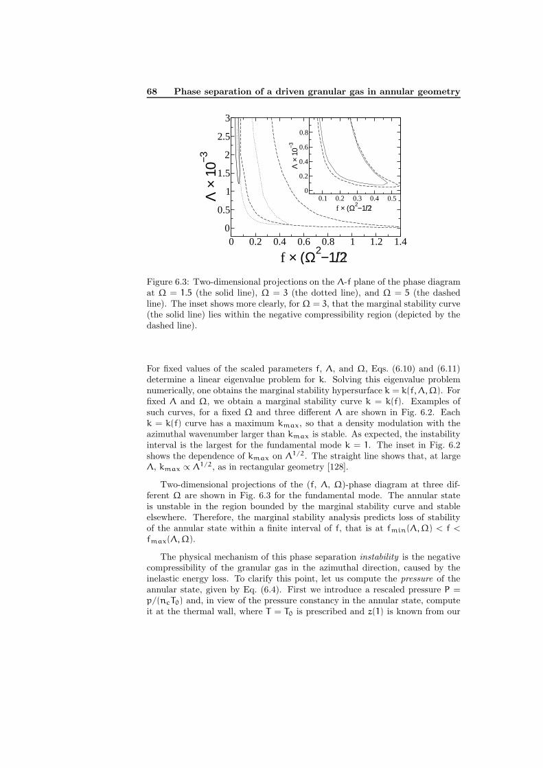
68 Phase separation of a driven granular gas in annular geometry
0 0.2 0.4 0.6 0.8 1 1.2 1.4
f × (Ω2−1)/2
0
0.5
1
1.5
2
2.5
3
Λ ×
10−3
0.1 0.2 0.3 0.4 0.5
f × (Ω2−1)/2
0
0.2
0.4
0.6
0.8
Λ ×
10−3
Figure 6.3: Two-dimensional projections on the Λ-f plane of the phase diagramat Ω = 1.5 (the solid line), Ω = 3 (the dotted line), and Ω = 5 (the dashedline). The inset shows more clearly, for Ω = 3, that the marginal stability curve(the solid line) lies within the negative compressibility region (depicted by thedashed line).
For fixed values of the scaled parameters f, Λ, and Ω, Eqs. (6.10) and (6.11)determine a linear eigenvalue problem for k. Solving this eigenvalue problemnumerically, one obtains the marginal stability hypersurface k = k(f, Λ, Ω). Forfixed Λ and Ω, we obtain a marginal stability curve k = k(f). Examples ofsuch curves, for a fixed Ω and three different Λ are shown in Fig. 6.2. Eachk = k(f) curve has a maximum kmax, so that a density modulation with theazimuthal wavenumber larger than kmax is stable. As expected, the instabilityinterval is the largest for the fundamental mode k = 1. The inset in Fig. 6.2shows the dependence of kmax on Λ1/2. The straight line shows that, at largeΛ, kmax ∝ Λ1/2, as in rectangular geometry [128].
Two-dimensional projections of the (f, Λ, Ω)-phase diagram at three dif-ferent Ω are shown in Fig. 6.3 for the fundamental mode. The annular stateis unstable in the region bounded by the marginal stability curve and stableelsewhere. Therefore, the marginal stability analysis predicts loss of stabilityof the annular state within a finite interval of f, that is at fmin(Λ, Ω) < f <
fmax(Λ, Ω).
The physical mechanism of this phase separation instability is the negativecompressibility of the granular gas in the azimuthal direction, caused by theinelastic energy loss. To clarify this point, let us compute the pressure of theannular state, given by Eq. (6.4). First we introduce a rescaled pressure P =
p/(ncT0) and, in view of the pressure constancy in the annular state, computeit at the thermal wall, where T = T0 is prescribed and z(1) is known from our
6.2 Particles in an annulus and granular hydrostatics 69
numerical solution for the annular state. We obtain
P(f, Λ, Ω) =1 + 2G(z(1))
z(1).
The spinodal (negative compressibility) region is determined by the necessarycondition for the instability : (∂P/∂f)Λ,Ω < 0, whereas the borders of the spin-odal region are defined by (∂P/∂f)Λ,Ω = 0. That is, computing the deriva-tive we arrive at ∂P/∂f = (∂P/∂z(1))(∂z(1)/∂z(Ω))(∂z(Ω)/∂f). One can easilycheck that the first and third multipliers on the righthand side of this relationare always negative, thus the sign of (∂P/∂f)Λ,Ω is determined by the sign of(∂z(1)/∂z(Ω))Λ,Ω.
Typical P(f) curves for a fixed Ω and several different Λ are shown in Fig. 6.4.One can see that, at sufficiently large Λ, the rescaled pressure P goes down withan increase of f at an interval f1 < f < f2. That is, the effective compressibilityof the gas with respect to a redistribution of the material in the azimuthaldirection is negative on this interval of area fractions. By joining the spinodalpoints f1 and (separately) f2 at different Λ, we can draw the spinodal linefor a fixed Ω. As Λ goes down, the spinodal interval shrinks and eventuallybecomes a point at a critical point (Pc, fc), or (Λc, fc) (where all the criticalvalues are Ω-dependent). For Λ < Λc P(f) monotonically increases and thereis no instability.
What is the relation between the spinodal interval (f1, f2) and the marginalstability interval (fmin, fmax)? These intervals would coincide were the az-imuthal wavelength of the perturbation infinite (or, equivalently, k → 0), sothat the azimuthal heat conduction would vanish. Of course, this is not possi-ble in annular geometry, where k ≥ 1. As a result, the negative compressibilityinterval must include in itself the marginal stability interval (fmin, fmax). Thisis what our calculations indeed show, see the inset of Fig. 6.3. That is, a neg-ative compressibility is necessary, but not sufficient, for instability, similarly towhat was found in rectangular geometry [128].
Importantly, the instability region of the parameter space is by no meansnot the whole region the region where phase separation is expected to occur.Indeed, in analogy to what happens in rectangular geometry [156, 160], phaseseparation is also expected in a binodal (or coexistence) region of the area frac-tions, where the annular state is stable to small perturbations, but unstable tosufficiently large ones. The whole region of phase separation should be largerthan the instability region, and it should of course include the instability re-gion. Though we did not attempt to determine the binodal region of the systemfrom the hydrostatic equations (this task has not been accomplished yet evenfor rectangular geometry, except in the close vicinity of the critical point [160]),we determined the binodal region from our molecular dynamics simulations re-ported in the next section.
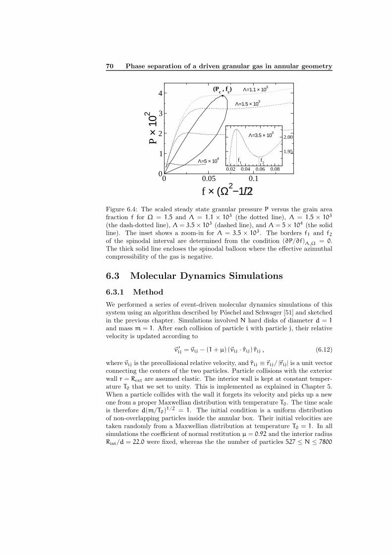
70 Phase separation of a driven granular gas in annular geometry
0 0.05 0.1
f × (Ω2−1)/2
0
1
2
3
4
P ×
102
0.02 0.04 0.06 0.08
1.95
2.00
Λ=1.1 × 10³
Λ=1.5 × 10³
Λ=3.5 × 10³
Λ=5 × 10⁴
(Pc , fc)
f1
f2
Figure 6.4: The scaled steady state granular pressure P versus the grain areafraction f for Ω = 1.5 and Λ = 1.1 × 10³ (the dotted line), Λ = 1.5 × 10³
(the dash-dotted line), Λ = 3.5 × 10³ (dashed line), and Λ = 5 × 10⁴ (the solidline). The inset shows a zoom-in for Λ = 3.5 × 10³. The borders f1 and f2
of the spinodal interval are determined from the condition (∂P/∂f)Λ,Ω = 0.The thick solid line encloses the spinodal balloon where the effective azimuthalcompressibility of the gas is negative.
6.3 Molecular Dynamics Simulations
6.3.1 Method
We performed a series of event-driven molecular dynamics simulations of thissystem using an algorithm described by Poschel and Schwager [51] and sketchedin the previous chapter. Simulations involved N hard disks of diameter d = 1
and mass m = 1. After each collision of particle i with particle j, their relativevelocity is updated according to
~v ′ij = ~vij − (1 + µ) (~vij · rij) rij , (6.12)
where ~vij is the precollisional relative velocity, and rij ≡ ~rij/ |~rij| is a unit vectorconnecting the centers of the two particles. Particle collisions with the exteriorwall r = Rext are assumed elastic. The interior wall is kept at constant temper-ature T0 that we set to unity. This is implemented as explained in Chapter 5.When a particle collides with the wall it forgets its velocity and picks up a newone from a proper Maxwellian distribution with temperature T0. The time scaleis therefore d(m/T0)1/2 = 1. The initial condition is a uniform distributionof non-overlapping particles inside the annular box. Their initial velocities aretaken randomly from a Maxwellian distribution at temperature T0 = 1. In allsimulations the coefficient of normal restitution µ = 0.92 and the interior radiusRint/d = 22.0 were fixed, whereas the the number of particles 527 ≤ N ≤ 7800
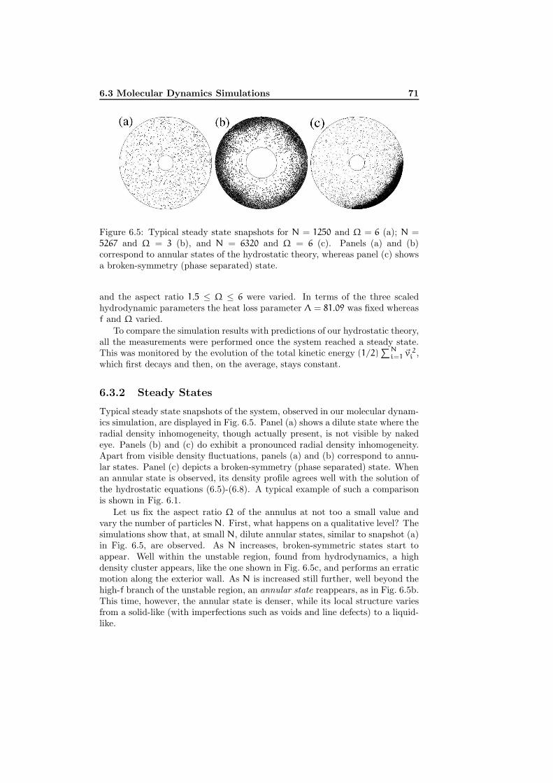
6.3 Molecular Dynamics Simulations 71
Figure 6.5: Typical steady state snapshots for N = 1250 and Ω = 6 (a); N =
5267 and Ω = 3 (b), and N = 6320 and Ω = 6 (c). Panels (a) and (b)correspond to annular states of the hydrostatic theory, whereas panel (c) showsa broken-symmetry (phase separated) state.
and the aspect ratio 1.5 ≤ Ω ≤ 6 were varied. In terms of the three scaledhydrodynamic parameters the heat loss parameter Λ = 81.09 was fixed whereasf and Ω varied.
To compare the simulation results with predictions of our hydrostatic theory,all the measurements were performed once the system reached a steady state.This was monitored by the evolution of the total kinetic energy (1/2)
∑Ni=1
~v 2i ,
which first decays and then, on the average, stays constant.
6.3.2 Steady States
Typical steady state snapshots of the system, observed in our molecular dynam-ics simulation, are displayed in Fig. 6.5. Panel (a) shows a dilute state where theradial density inhomogeneity, though actually present, is not visible by nakedeye. Panels (b) and (c) do exhibit a pronounced radial density inhomogeneity.Apart from visible density fluctuations, panels (a) and (b) correspond to annu-lar states. Panel (c) depicts a broken-symmetry (phase separated) state. Whenan annular state is observed, its density profile agrees well with the solution ofthe hydrostatic equations (6.5)-(6.8). A typical example of such a comparisonis shown in Fig. 6.1.
Let us fix the aspect ratio Ω of the annulus at not too a small value andvary the number of particles N. First, what happens on a qualitative level? Thesimulations show that, at small N, dilute annular states, similar to snapshot (a)in Fig. 6.5, are observed. As N increases, broken-symmetric states start toappear. Well within the unstable region, found from hydrodynamics, a highdensity cluster appears, like the one shown in Fig. 6.5c, and performs an erraticmotion along the exterior wall. As N is increased still further, well beyond thehigh-f branch of the unstable region, an annular state reappears, as in Fig. 6.5b.This time, however, the annular state is denser, while its local structure variesfrom a solid-like (with imperfections such as voids and line defects) to a liquid-like.
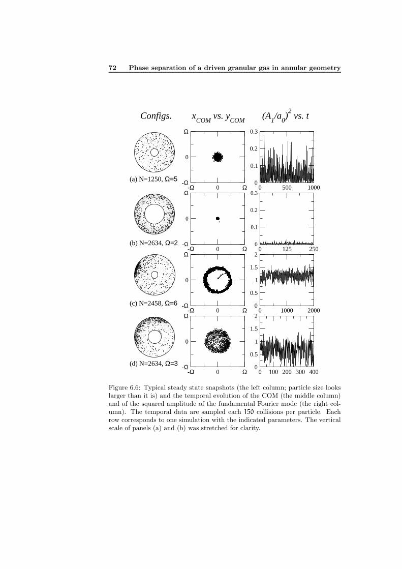
72 Phase separation of a driven granular gas in annular geometry
-Ω Ω0-Ω
Ω
0
0 500 10000
0.1
0.2
0.3
-Ω 0 Ω-Ω
0
Ω
0 100 200 300 4000
0.5
1
1.5
2-Ω 0 Ω
-Ω
Ω
0
0 1000 20000
0.5
1
1.5
2-Ω 0 Ω
-Ω
0
Ω
0 125 2500
0.1
0.2
0.3
(a) N=1250, Ω=5
(b) N=2634, Ω=2
(c) N=2458, Ω=6
(d) N=2634, Ω=3
Configs. xCOM
vs. yCOM
(A1/a
0)2 vs. t
Figure 6.6: Typical steady state snapshots (the left column; particle size lookslarger than it is) and the temporal evolution of the COM (the middle column)and of the squared amplitude of the fundamental Fourier mode (the right col-umn). The temporal data are sampled each 150 collisions per particle. Eachrow corresponds to one simulation with the indicated parameters. The verticalscale of panels (a) and (b) was stretched for clarity.
6.3 Molecular Dynamics Simulations 73
To characterize the spatio-temporal behavior of the granulate at a steadystate, we followed the position of the center of mass (COM) of the granulate.Several examples of the COM trajectories are displayed in Fig. 6.6. Here cases(a) and (b) correspond, in the hydrodynamic language, to annular states. Thereare, however, significant fluctuations of the COM around the center of the an-nulus. These fluctuations are of course not accounted for by hydrodynamictheory. In case (b), where the dense cluster develops, the fluctuations are muchweaker that in case (a). More interesting are cases (c) and (d). They corre-spond to broken-symmetry states: well within the phase separation region ofthe parameter space (case c) and close to the phase separation border (cased). The COM trajectory in case (c) shows that the granular “droplet” per-forms random motion in the azimuthal direction, staying close to the exteriorwall. This is in contrast with case (d), where fluctuations are strong both in theazimuthal and in the radial directions. Following the actual snapshots of thesimulation, one observes here a very complicated motion of the “droplet”, aswell as its dissolution into more “droplets”, mergers of the droplets etc. There-fore, as in the case of granular phase separation in rectangular geometry [148],the granular phase separation in annular geometry is accompanied by consider-able spatio-temporal fluctuations. In this situation a clear distinction betweena phase-separated state and an annular state, and a comparison between thesimulations and hydrodynamic theory, demand proper diagnostics. We foundthat such diagnostics are provided by the azimuthal spectrum of the particledensity and its probability distribution.
6.3.3 Azimuthal Density Spectrum
Let us consider the (time-dependent) rescaled density field ν(r, θ, t) = n(r, θ, t)/nc
(where r is rescaled to the interior wall radius as before), and introduce the in-tegrated field ν(θ, t):
ν(θ, t) =
∫Ω
1
ν(r, θ, t) r dr . (6.13)
In a system of N particles, ν(θ, t) is normalized so that
∫2π
0
ν(θ, t) dθ =N
nc R2int
. (6.14)
Because of the periodicity in θ the function ν(θ, t) can be expanded in a Fourierseries:
ν(θ, t) = a0 +
∞∑
k=1
[ak(t) cos(kθ) + bk(t) sin(kθ)] , (6.15)
where a0 is independent of time because of the normalization condition (6.14).We will work with the quantities
A2k(t) ≡ a2
k(t) + b2k(t) , k ≥ 1 . (6.16)
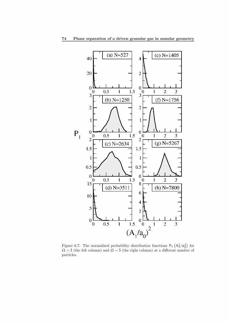
74 Phase separation of a driven granular gas in annular geometry
Figure 6.7: The normalized probability distribution functions P1
(
A21/a2
0
)
forΩ = 3 (the left column) and Ω = 5 (the right column) at a different number ofparticles.

6.3 Molecular Dynamics Simulations 75
Table 6.1: The averaged squared relative amplitudes 〈A2k(t)〉/a2
0 for the firstthree modes k = 1, 2 and 3. (a) N = 2634, Ω = 3, (b) N = 5267, Ω = 4, (c)N = 1000, Ω = 2.25, and (d) N = 1250, Ω = 3.
k (a) (b) (c) (d)
1 0.66 ± 0.05 0.39 ± 0.04 0.30 ± 0.08 0.77 ± 0.05
2 0.04 ± 0.02 0.05 ± 0.02 0.07 ± 0.01 0.28 ± 0.09
3 0.03 ± 0.02 0.03 ± 0.03 0.02 ± 0.02 0.11 ± 0.08
For the (deterministic) annular state one has Ak = 0 for all k ≥ 1, while for asymmetry-broken state Ak > 0. The relative quantities A2
k(t)/a20 can serve as
measures of the azimuthal symmetry breaking. As is shown in Table 6.1, A21(t)
is usually much larger (on the average) that the rest of A2k(t). Therefore, the
quantity A21(t)/a2
0 is sufficient for our purposes.
Once the system relaxed to a steady state, we followed the temporal evolutionof the quantity A2
1/a20. Typical results are shown in the right column of Fig. 6.6.
One observes that, for annular states, this quantity is usually small, as is thecases (a) and (b) in Fig. 6.6. For broken-symmetry states A2
1 is larger, and itincreases as one moves deeper into the phase separation region. (Notice thatthe averaged value of A2
1/a20 in (c) is larger than in (d), which means that (c) is
deeper in the phase separation region.) Another characteristics of A21(t)/a2
0 isthe magnitude of fluctuations. One can notice that, in the vicinity of the phaseseparation border the fluctuations are stronger (as in case (d) in Fig. 6.6).
All these properties are encoded in the probability distribution P1 of thevalues of (A1/a0)
2: the ultimate tool of our diagnostics. Figure 6.7 showstwo series of measurements of this quantity at different N: for Ω = 3 andΩ = 5. By following the position of the maximum of P1 we were able to tosharply discriminate between the annular states and phase separated states andtherefore to locate the phase separation border. When the maximum of P1
occurs at the zero value of (A1/a0)2 (as in cases (a) and (d) and, respectively,
(e) and (h) in Fig. 6.7), an annular state is observed. On the contrary, when
the maximum of P1 occurs at a non-zero value of (A1/a0)2
(as in cases (b)and (c) and, respectively, (f) and (g) in Fig. 6.7), a phase separated state isobserved. In each case, the width of the probability distribution (measured,for example, at the half-maximum) yields a direct measure of the magnitudeof fluctuations. Near the phase separation border, strong fluctuations (that is,broader distributions) are observed, as in case (c) of Fig. 6.7.
Using the position of the maximum of P1 as a criterion for phase separation,we show, in Fig. 6.8, the Ω − f diagram obtained from the molecular dynamicssimulations. The same figure also depicts the hydrostatic prediction of theinstability region. One can see that the instability region is located within thephase separation region, as expected.
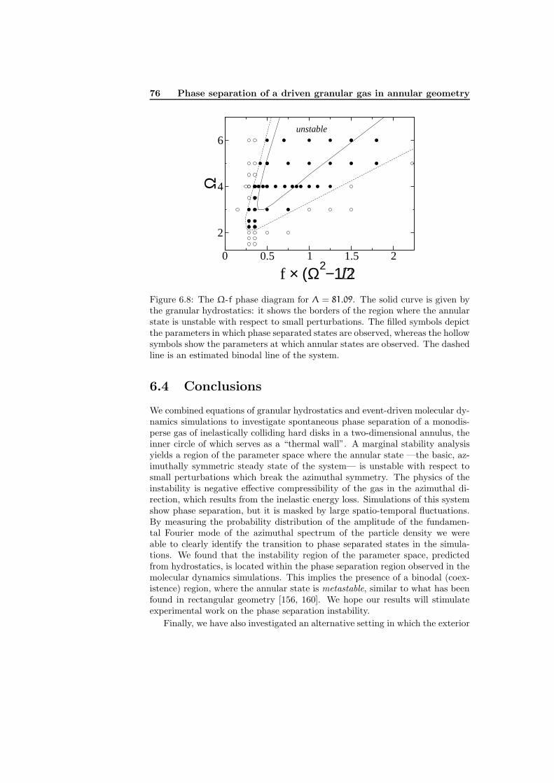
76 Phase separation of a driven granular gas in annular geometry
0 0.5 1 1.5 2
f × (Ω2−1)/2
2
4
6
Ω
unstable
Figure 6.8: The Ω-f phase diagram for Λ = 81.09. The solid curve is given bythe granular hydrostatics: it shows the borders of the region where the annularstate is unstable with respect to small perturbations. The filled symbols depictthe parameters in which phase separated states are observed, whereas the hollowsymbols show the parameters at which annular states are observed. The dashedline is an estimated binodal line of the system.
6.4 Conclusions
We combined equations of granular hydrostatics and event-driven molecular dy-namics simulations to investigate spontaneous phase separation of a monodis-perse gas of inelastically colliding hard disks in a two-dimensional annulus, theinner circle of which serves as a “thermal wall”. A marginal stability analysisyields a region of the parameter space where the annular state —the basic, az-imuthally symmetric steady state of the system— is unstable with respect tosmall perturbations which break the azimuthal symmetry. The physics of theinstability is negative effective compressibility of the gas in the azimuthal di-rection, which results from the inelastic energy loss. Simulations of this systemshow phase separation, but it is masked by large spatio-temporal fluctuations.By measuring the probability distribution of the amplitude of the fundamen-tal Fourier mode of the azimuthal spectrum of the particle density we wereable to clearly identify the transition to phase separated states in the simula-tions. We found that the instability region of the parameter space, predictedfrom hydrostatics, is located within the phase separation region observed in themolecular dynamics simulations. This implies the presence of a binodal (coex-istence) region, where the annular state is metastable, similar to what has beenfound in rectangular geometry [156, 160]. We hope our results will stimulateexperimental work on the phase separation instability.
Finally, we have also investigated an alternative setting in which the exterior
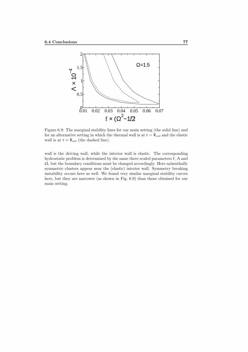
6.4 Conclusions 77
0.01 0.02 0.03 0.04 0.05 0.06 0.07
f × (Ω2−1)/2
0
0.5
1
1.5
2
Λ ×
10−4
Ω=1.5
Figure 6.9: The marginal stability lines for our main setting (the solid line) andfor an alternative setting in which the thermal wall is at r = Rext and the elasticwall is at r = Rint (the dashed line).
wall is the driving wall, while the interior wall is elastic. The correspondinghydrostatic problem is determined by the same three scaled parameters f, Λ andΩ, but the boundary conditions must be changed accordingly. Here azimuthallysymmetric clusters appear near the (elastic) interior wall. Symmetry breakinginstability occurs here as well. We found very similar marginal stability curveshere, but they are narrower (as shown in Fig. 6.9) than those obtained for ourmain setting.

78 Phase separation of a driven granular gas in annular geometry
Chapter 7
Close–packed granular
clusters
Dense granular clusters often behave like macro-particles. We address this inter-esting phenomenon in a model system of inelastically colliding hard disks insidea circular box, driven by a thermal wall at zero gravity. Molecular dynam-ics simulations show a close-packed cluster of an almost circular shape, weaklyfluctuating in space and isolated from the driving wall by a low-density gas.The density profile of the system agrees well with the azimuthally symmetricsolution of granular hydrostatic equations employing constitutive relations byGrossman et al. We find that fluctuations of the center of mass of the system areGaussian. This suggests an effective Langevin description in terms of a macro-particle, confined by a harmonic potential and driven by a delta-correlated noise.Surprisingly, the fluctuations persist when increasing the number of particles inthe system.
7.1 Introduction
This chapter addresses granular hydrodynamics and fluctuations in a simpletwo–dimensional granular system under conditions when existing hydrodynamicdescriptions [140, 141, 142] break down because of large density, not large in-elasticity. In view of the difficulties mentioned in Chapters 5 and 6, attempts ofa first–principle description of hydrodynamics and fluctuations should give wayhere to more practical, empiric or semi–empiric, approaches. One such approachto a hydrodynamic (or, rather, hydrostatic) description was suggested by Gross-man et al. [154]. In the present chapter, we put it into a test in an extremecase when macro–particles (granular clusters with the maximum density closeto the hexagonal close packing) form. The model system we are dealing withwas first introduced by Esipov and Poschel [153]. It is an assembly of N 1
identical disks of mass m, diameter d and coefficient of normal restitution µ,placed inside a circular box of radius R at zero gravity (typical steady state
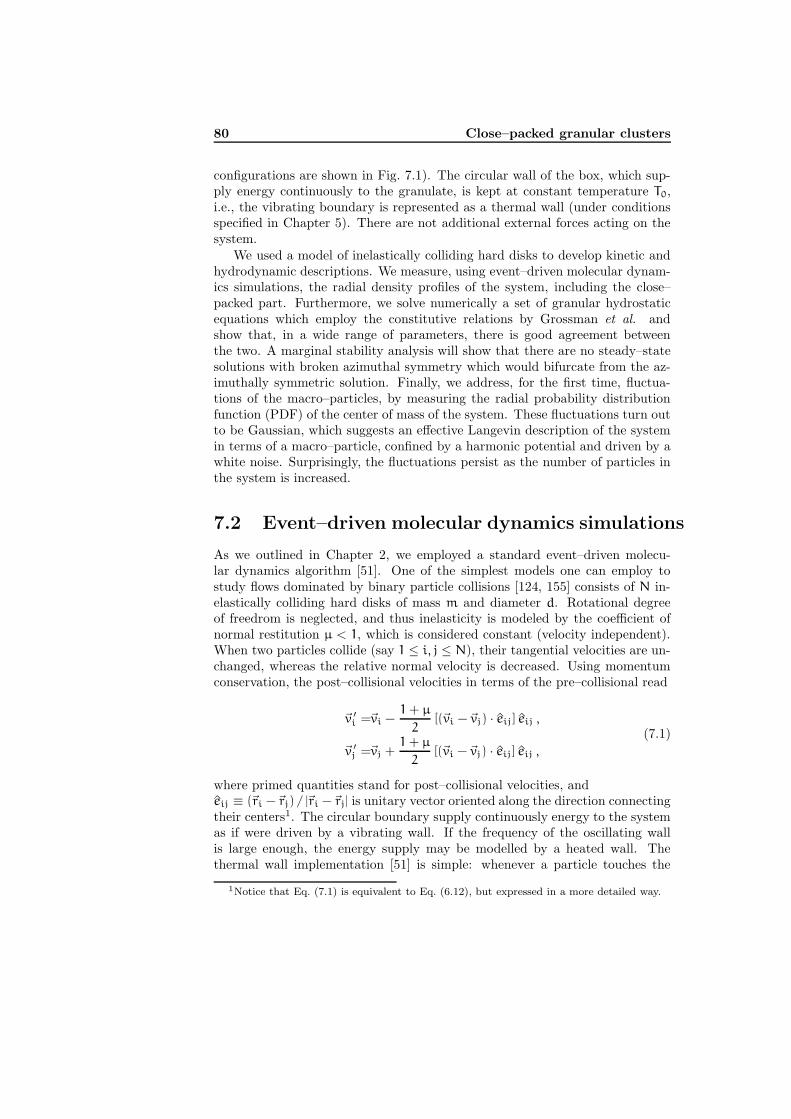
80 Close–packed granular clusters
configurations are shown in Fig. 7.1). The circular wall of the box, which sup-ply energy continuously to the granulate, is kept at constant temperature T0,i.e., the vibrating boundary is represented as a thermal wall (under conditionsspecified in Chapter 5). There are not additional external forces acting on thesystem.
We used a model of inelastically colliding hard disks to develop kinetic andhydrodynamic descriptions. We measure, using event–driven molecular dynam-ics simulations, the radial density profiles of the system, including the close–packed part. Furthermore, we solve numerically a set of granular hydrostaticequations which employ the constitutive relations by Grossman et al. andshow that, in a wide range of parameters, there is good agreement betweenthe two. A marginal stability analysis will show that there are no steady–statesolutions with broken azimuthal symmetry which would bifurcate from the az-imuthally symmetric solution. Finally, we address, for the first time, fluctua-tions of the macro–particles, by measuring the radial probability distributionfunction (PDF) of the center of mass of the system. These fluctuations turn outto be Gaussian, which suggests an effective Langevin description of the systemin terms of a macro–particle, confined by a harmonic potential and driven by awhite noise. Surprisingly, the fluctuations persist as the number of particles inthe system is increased.
7.2 Event–driven molecular dynamics simulations
As we outlined in Chapter 2, we employed a standard event–driven molecu-lar dynamics algorithm [51]. One of the simplest models one can employ tostudy flows dominated by binary particle collisions [124, 155] consists of N in-elastically colliding hard disks of mass m and diameter d. Rotational degreeof freedrom is neglected, and thus inelasticity is modeled by the coefficient ofnormal restitution µ < 1, which is considered constant (velocity independent).When two particles collide (say 1 ≤ i, j ≤ N), their tangential velocities are un-changed, whereas the relative normal velocity is decreased. Using momentumconservation, the post–collisional velocities in terms of the pre–collisional read
~v ′i =~vi −
1 + µ
2[(~vi −~vj) · eij] eij ,
~v ′j =~vj +
1 + µ
2[(~vi −~vj) · eij] eij ,
(7.1)
where primed quantities stand for post–collisional velocities, andeij ≡ (~ri −~rj) / |~ri −~rj| is unitary vector oriented along the direction connectingtheir centers1. The circular boundary supply continuously energy to the systemas if were driven by a vibrating wall. If the frequency of the oscillating wallis large enough, the energy supply may be modelled by a heated wall. Thethermal wall implementation [51] is simple: whenever a particle touches the
1Notice that Eq. (7.1) is equivalent to Eq. (6.12), but expressed in a more detailed way.
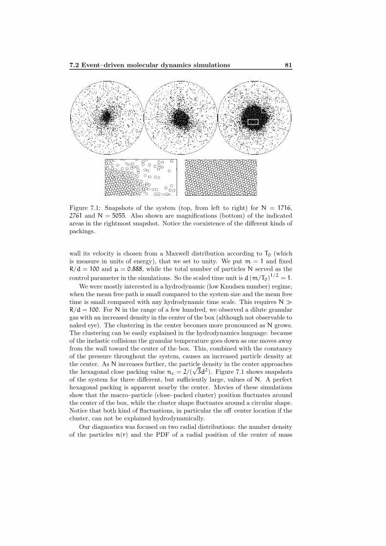
7.2 Event–driven molecular dynamics simulations 81
Figure 7.1: Snapshots of the system (top, from left to right) for N = 1716,2761 and N = 5055. Also shown are magnifications (bottom) of the indicatedareas in the rightmost snapshot. Notice the coexistence of the different kinds ofpackings.
wall its velocity is chosen from a Maxwell distribution according to T0 (whichis measure in units of energy), that we set to unity. We put m = 1 and fixedR/d = 100 and µ = 0.888, while the total number of particles N served as the
control parameter in the simulations. So the scaled time unit is d (m/T0)1/2
= 1.
We were mostly interested in a hydrodynamic (low Knudsen number) regime,when the mean free path is small compared to the system size and the mean freetime is small compared with any hydrodynamic time scale. This requires N R/d = 100. For N in the range of a few hundred, we observed a dilute granulargas with an increased density in the center of the box (although not observable tonaked eye). The clustering in the center becomes more pronounced as N grows.The clustering can be easily explained in the hydrodynamics language: becauseof the inelastic collisions the granular temperature goes down as one moves awayfrom the wall toward the center of the box. This, combined with the constancyof the pressure throughout the system, causes an increased particle density atthe center. As N increases further, the particle density in the center approachesthe hexagonal close packing value nc = 2/(
√3d2). Figure 7.1 shows snapshots
of the system for three different, but sufficiently large, values of N. A perfecthexagonal packing is apparent nearby the center. Movies of these simulationsshow that the macro–particle (close–packed cluster) position fluctuates aroundthe center of the box, while the cluster shape fluctuates around a circular shape.Notice that both kind of fluctuations, in particular the off–center location if thecluster, can not be explained hydrodynamically.
Our diagnostics was focused on two radial distributions: the number densityof the particles n(r) and the PDF of a radial position of the center of mass

82 Close–packed granular clusters
of the system P(rm), defined below. To measure n(r) (likewise in Chapter 6),we recorded all particle coordinates in intervals of 100, 000 particle collisions.For each snapshot we introduced bins in the form of concentric circular ringsof width 0.5, centered in the center of mass of the system. For each particlewe determined the fraction of its area falling in each of the rings, summed thecontributions of all particles to each bin, and divided the result by the bin area.The resulting radial profile was averaged over many snapshots (typically 1000).Similar method is employed to measure P(rm). As we are interested in steady–state distributions, we disregarded initial transients. This was monitored by thetime–dependence of the average kinetic energy of the particles (the first decayedand then approached an almost constant value) and the time–dependence of thecenter of mass itself.
7.3 Hydrostatic theory
As the fluctuations are relatively weak, it is natural to start with a purelyhydrodynamic description. For a zero mean flow this is a hydrostatic theory,as it operates only with (time–independent) granular density n(r), temperatureT(r) and pressure p(r). The energy input at the thermal wall is balanced bydissipation due to inter–particle collisions, and one can employ the momentumand energy balance equations:
p = const ,
∇ · (κ∇T) = I .(7.2)
Here κ is the thermal conductivity and I is the rate of energy loss by collisions.Note that the heat flux, entering the thermal balance in Eq. (7.2), does notinclude an inelastic term, proportional to the density gradient [140, 141, 142].In the nearly elastic limit 1 − µ 1, that we are interested in, this term canbe neglected. The boundary condition at the thermal wall is T(r = R, θ) = T0,where r and θ are polar coordinates with the origin at the center of the box.
To proceed from here and compute numerical factors, we need constitutiverelations: an equation of state p = p (n, T) and relations for κ and I in termsof n and T . As we attempt to describe close–packed clusters, the first–principlestandard techniques, based on the Boltzmann or Enskog equations, are inap-plicable. Grossman et al. [154] suggested a set of semi–empiric relations intwo dimensions, that are valid for all densities, all the way to hexagonal closepacking. Their approach ignores possible coexistence beyond the disorder–ordertransition and assumes that the whole system is on the thermodynamic branchextending to the hexagonal close packing. The delicate issue of phase coexis-tence (liquid–like phase, close–packed phase with multiple domains) occur hereis close analogy to the system of elastic hard spheres [122, 144, 164]. Gross-man et al. employed free volume arguments in the vicinity of the close packing,and suggested an interpolation between the hexagonal–packing limit and thewell–known low–density relations. The resulting global equation of state and
7.3 Hydrostatic theory 83
constitutive relations [154] read
p = n Tnc + n
nc − n,
κ =σ n (αl + d)2T1/2
l,
I = (σ/γl) (1 − µ2) n T3/2 .
(7.3)
Here l is the mean free path, which is given by an interpolation formula [154]
l =1√8nd
nc − n
nc − an, (7.4)
and a = 1 − (3/8)1/2 . These relations include three dimensionless numericalfactors of order unity: α, γ and σ, where the latter drops out from the steady–state problem. They can be calculated exactly from the velocity distributionfunction. However, this distribution is poorly understood [124]. Grossman etal. determined the optimum values α = 1.15 and γ = 2.26, verified by adetailed comparison with molecular dynamics simulations of a system of inelastichard disks in a rectangular box without gravity, driven by a thermal wall, andnumerical solutions of the hydrostatic equations (7.2) in rectangular geometry.We adopted the same values of α2 and γ in our calculations for the circulargeometry.
Most interesting state among the one–dimensional states is the azimuthallysymmetric state (θ–independent), which is indeed one of the possible solutionsof Eq. (7.2). In this case, assuming azimuthal symmetry, we rewrite Eq. (7.2)as
p(n, T) = const ,
1
r
d
dr
[
r κ(n, T)dT
dr
]
= I(n, T) .(7.5)
Equations (7.5) can be reduced to a single equation for the scaled inverse densityz(r) ≡ nc/n(r). In the rescaled coordinate, r/R → r, the circle radius becomes1, and Eqs. (7.5) reduces to
1
r
d
dr
[
rF(z)dz
dr
]
= ΛQ(z) , (7.6)
where
F(z) =(z2 + 2z − 1)
[
αz(z − 1) +√
32/3(z − a)]2
(z − a)(z − 1)1/2z3/2(z + 1)5/2
Q(z) =(z − a)(z − 1)1/2
(z + 1)3/2z1/2,
(7.7)
2The value of α differs in systems with gravity (α ≈ 0.6) [130].

84 Close–packed granular clusters
0
0.5
1
0 0.5 1r/R
0
0.5
1
n/n c
0 0.5 1
N=1716 N=2077
N=2761 N=5055
Figure 7.2: Scaled density n/nc versus scaled radius r/R as observed in simu-lations (circles) and predicted by the hydrostatic theory with the constitutiverelations by Grossman et al. [154] (solid lines) and with the Enskog-type rela-tions [135] (dashed lines) for four different values of the total number of particlesN. For the rest of parameters please see the text. The dotted lines indicaten/nc = 1.
7.3 Hydrostatic theory 85
and Λ = (32/3γ) (R/d)2 (1 − µ2) is the hydrodynamic inelasticity parameter,first introduced in Ref. [159] in the context of rectangular geometry 3. The fixedtotal number of particles yields a normalization condition, which read
∫1
0
z−1(r) r dr = f/2 , (7.8)
where f = (√
3/2π)N(d/R)2 is the average grain area fraction. Equations (7.6)and (7.8), together with the obvious boundary condition dz/dr|r=0 = 0 (thisis a consequence of the fact that the temperature gradient vanish at the centerof the system), form a complete set. The hydrostatic problem is completelydetermined by two scaled parameters Λ and f. This can be solved numericallyas explained in Chapter 6 for the annular geometry. That is, in order to solveEq. (7.6), instead of consider the area fraction f one can prescribe the inversedensity at the center of the system z0. This condition, combined with the no–flux condition at r = 0 define a Cauchy problem for z−1(r) [128]. Solving theCauchy problem one can compute the respective value for f from Eq. (7.8). Atfixed Λ, z0 is a strictly monotonically decreasing function of f. Therefore, analternative parameterization of the azimuthally symmetric state is given by thescaled numbers Λ and z0. The same considerations keep for the marginal sta-bility analysis (see below).
In our event–driven simulations we varied the number of particles N. Accord-ingly, the scaled parameter f is varied, while Λ = 9980 was constant. Figure 7.2shows a comparison of the hydrostatic radial density profiles with the radialdensity profiles obtained in simulations, for four different values of N. The sim-ulations profiles were averaged over 1000 uncorrelated configurations. It can beseen from Fig. 7.2 that for N = 1716 the theory overestimates the density inthe center of the box. This is expected as, for relatively small N, the maximumdensity is considerably less than the close–packing density, and the accuracyof the constitutive relations by Grossman et al. is not as good. For larger N
the agreement rapidly improves. As Fig. 7.3 shows, the agreement between thehydrostatic theory and the simulations persists for the maximum radial den-sities at different number of particles N. The agreement is excellent for thedensities approaching the close packing density, whereas for small N, there issmall deviations. In absolute scale, however, the agreement is very good. Wealso computed the density profiles using another set of semi-empiric constitutiverelations4, those obtained in the spirit of Enskog theory [135]. These read,
κ =2dnT1/2G
π1/2
[
1 +9π
16
(
1 +2
3G
)2]
,
I =8(1 − µ)nT3/2G
d√
π,
(7.9)
3Notice that, no matter how small (but finite) the inelasticity is, the parameter Λ goes toinfinity in the thermodynamic limit R → ∞.
4These were already employed in Chapter 6.

86 Close–packed granular clusters
2000 4000 6000N
0
0.2
0.4
0.6
0.8
1
n max
/nc
MD simulationsHydrostatics
Figure 7.3: Maximum scaled density nmax/nc as a function of N as predictedby the hydrostatic theory and observed in simulations.
and the equation of state first proposed by Carnahan and Starling [162]
P = nT(1 + 2G) , (7.10)
where G = ν(1 − 7ν16
)/(1 − ν)2 and ν = n(
πd2/4)
is the solid fraction. Onecan clearly see from Fig. 7.2 that the Enskog-type constitutive relations predictunphysically high densities in the cluster.
We employ the same hydrostatic formulation to perform a systematic linearstability analysis of the reference state (azimuthally symmetric solution). Inthe framework of time–dependent hydrodynamics, this corresponds to marginalstability analysis of the azimuthally symmetric solution with respect to smallperturbations along the azimuthal coordinate θ. Substituting
z(r, θ) = z(r) + ε φk(r) sin(k θ) , (7.11)
where k ≥ 1 is an integer, into Eq. (7.2) and linearizing around the azimuthallysymmetric state z(r) with respect to the small correction ε 1, we arrive to alinear eigenvalue problem for k = k(f) which read
ζ′′k +1
rζ′k −
[
k2
r2+
ΛQ′(z)
F(z)
]
ζk = 0 , (7.12)
where ζk(r) = φk(r)F(z). This equation is complemented by the boundaryconditions
ζk(0) = 0 ζk(1) = 0 . (7.13)
For a fixed value of Λ, we obtain numerically the marginal stability curvek = k(f) and the corresponding eigenfunctions ζk by analyzing (as explained in
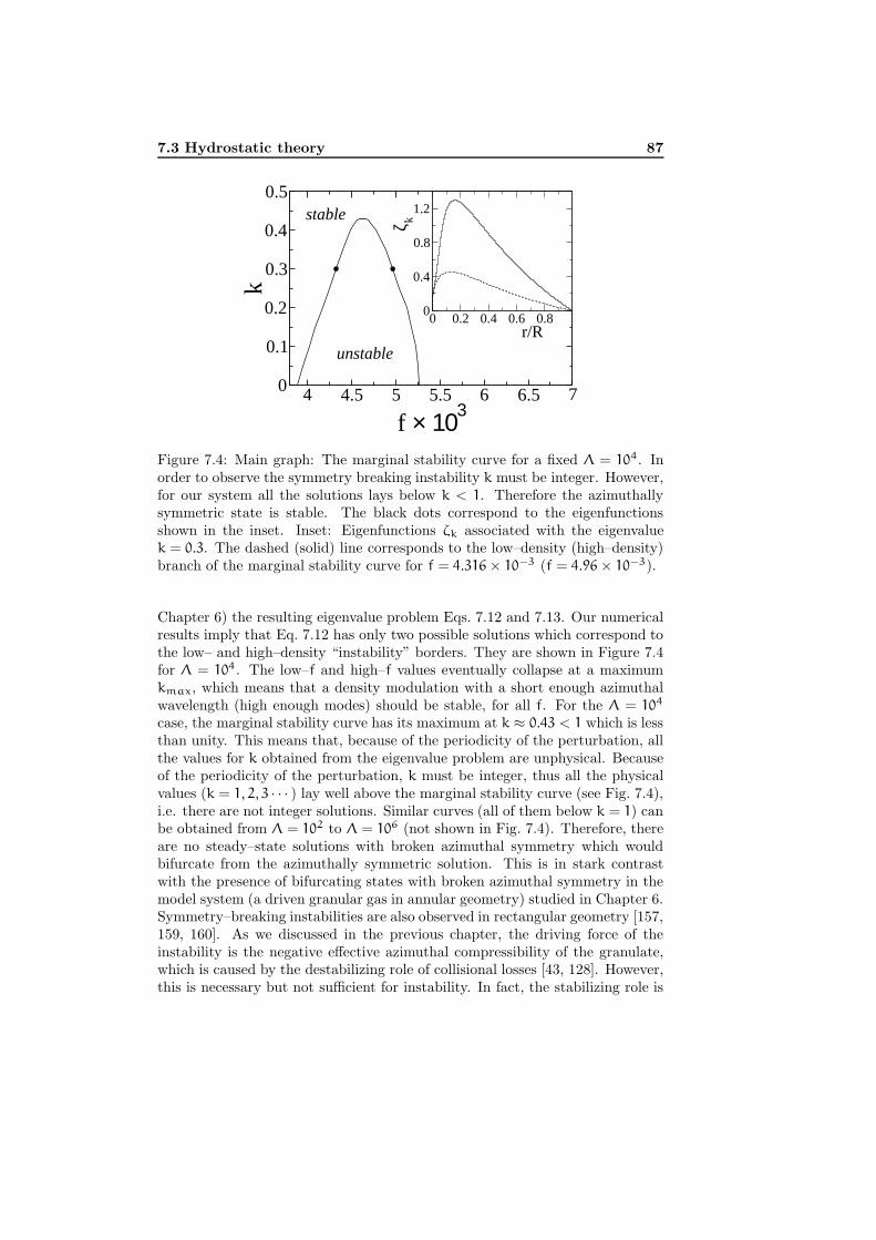
7.3 Hydrostatic theory 87
4 5 6 76.55.54.5
f × 1030
0.1
0.2
0.3
0.4
0.5
k
0 0.2 0.4 0.6 0.8r/R
0
0.4
0.8
1.2
ζ kstable
unstable
Figure 7.4: Main graph: The marginal stability curve for a fixed Λ = 104. Inorder to observe the symmetry breaking instability k must be integer. However,for our system all the solutions lays below k < 1. Therefore the azimuthallysymmetric state is stable. The black dots correspond to the eigenfunctionsshown in the inset. Inset: Eigenfunctions ζk associated with the eigenvaluek = 0.3. The dashed (solid) line corresponds to the low–density (high–density)branch of the marginal stability curve for f = 4.316 × 10⁻³ (f = 4.96 × 10⁻³).
Chapter 6) the resulting eigenvalue problem Eqs. 7.12 and 7.13. Our numericalresults imply that Eq. 7.12 has only two possible solutions which correspond tothe low– and high–density “instability” borders. They are shown in Figure 7.4for Λ = 104. The low–f and high–f values eventually collapse at a maximumkmax, which means that a density modulation with a short enough azimuthalwavelength (high enough modes) should be stable, for all f. For the Λ = 104
case, the marginal stability curve has its maximum at k ≈ 0.43 < 1 which is lessthan unity. This means that, because of the periodicity of the perturbation, allthe values for k obtained from the eigenvalue problem are unphysical. Becauseof the periodicity of the perturbation, k must be integer, thus all the physicalvalues (k = 1, 2, 3 · · · ) lay well above the marginal stability curve (see Fig. 7.4),i.e. there are not integer solutions. Similar curves (all of them below k = 1) canbe obtained from Λ = 102 to Λ = 106 (not shown in Fig. 7.4). Therefore, thereare no steady–state solutions with broken azimuthal symmetry which wouldbifurcate from the azimuthally symmetric solution. This is in stark contrastwith the presence of bifurcating states with broken azimuthal symmetry in themodel system (a driven granular gas in annular geometry) studied in Chapter 6.Symmetry–breaking instabilities are also observed in rectangular geometry [157,159, 160]. As we discussed in the previous chapter, the driving force of theinstability is the negative effective azimuthal compressibility of the granulate,which is caused by the destabilizing role of collisional losses [43, 128]. However,this is necessary but not sufficient for instability. In fact, the stabilizing role is
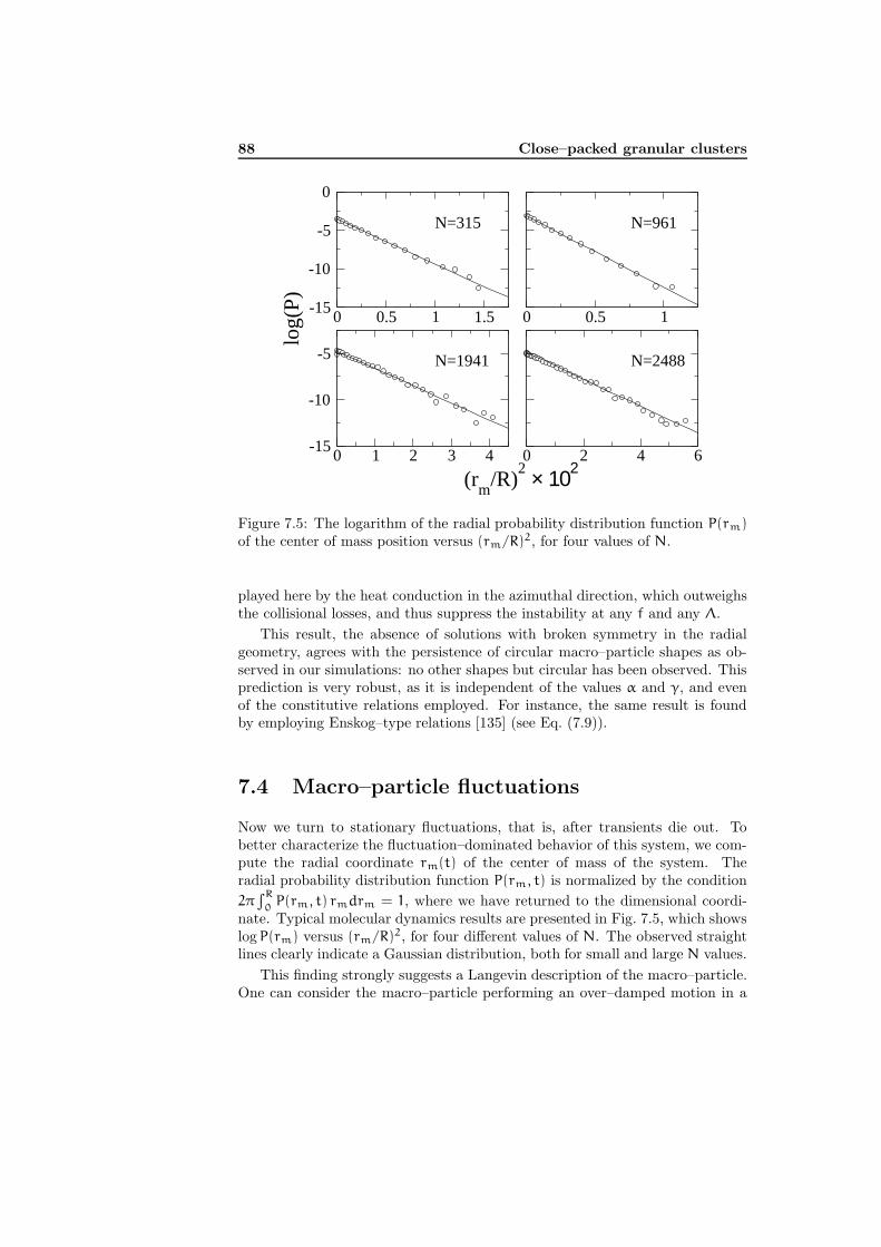
88 Close–packed granular clusters
0 0.5 1 1.5-15
-10
-5
0
0 0.5 1
0 1 2 3 4
(rm
/R)2 × 102
-15
-10
-5
log(
P)
0 2 4 6
N=315 N=961
N=1941 N=2488
Figure 7.5: The logarithm of the radial probability distribution function P(rm)
of the center of mass position versus (rm/R)2, for four values of N.
played here by the heat conduction in the azimuthal direction, which outweighsthe collisional losses, and thus suppress the instability at any f and any Λ.
This result, the absence of solutions with broken symmetry in the radialgeometry, agrees with the persistence of circular macro–particle shapes as ob-served in our simulations: no other shapes but circular has been observed. Thisprediction is very robust, as it is independent of the values α and γ, and evenof the constitutive relations employed. For instance, the same result is foundby employing Enskog–type relations [135] (see Eq. (7.9)).
7.4 Macro–particle fluctuations
Now we turn to stationary fluctuations, that is, after transients die out. Tobetter characterize the fluctuation–dominated behavior of this system, we com-pute the radial coordinate rm(t) of the center of mass of the system. Theradial probability distribution function P(rm, t) is normalized by the condition
2π∫R
0P(rm, t) rmdrm = 1, where we have returned to the dimensional coordi-
nate. Typical molecular dynamics results are presented in Fig. 7.5, which showslog P(rm) versus (rm/R)2, for four different values of N. The observed straightlines clearly indicate a Gaussian distribution, both for small and large N values.
This finding strongly suggests a Langevin description of the macro–particle.One can consider the macro–particle performing an over–damped motion in a
7.5 Conclusions 89
(central–symmetric) confining harmonic potential5 U(rm) = kr2m/2 and driven
by a (delta–correlated) discrete–particle noise η(t). The Langevin equation forthis problem reads
hrm + krm = η(t) , (7.14)
where h is the damping rate, 〈η(t)η(t′)〉 = 2hΓ δ(t − t′), and Γ is an effectivemagnitude of the discrete–particle noise. In the simplest approach the close–packed cluster and the discrete–particle noise can be characterized, for each N,respectively, by a point–like mass M and mobility χ, and by T0, the temperatureof the circular wall. A stochastic equivalent description is provided in termsof the Fokker-Planck equation for P(rm, t) [1, 2]. In the limit Γ → 0, the(deterministic) steady-state solution of Eq. (7.14) is rm = rm = 0: the macro–particle at rest, located at the center of the box. At Γ > 0, the steady statedistribution function is given by the steady state solution of the Fokker-Planckequation [1, 2] which is P(rm) = (π σ2)−1 exp(−r2
m/σ2), where σ2 = Γ/k, andthe normalization constant is computed for σ R. The variance σ2 is the ratioof Γ (a characteristic of the discrete noise) and k (a macroscopic quantity). Animportant insight can be achieved from the N–dependence of σ, obtained bymolecular dynamics (see Section 7.2). In analogy with equilibrium systems, onemight expect the relative magnitude of fluctuations to decrease with increasingN. Surprisingly, this is not what we observed, see Fig. 7.6. One can see thatσ(N) approaches a plateau, that is fluctuations persist at large N. The small–N
behavior (the first three data points: N = 150, 315 and 480) in Fig. 7.6 agreeswith the dependence σ/R = O(N−1/2), expected for an ideal gas in equilibrium.Not surprisingly, for these relatively small N the clustering effect is small. On theother hand, at very large N, when the whole system approaches close packing(in our event–driven simulations, this corresponds to N = 36275), σ/R mustgo to zero. We could not probe this regime, however, as simulations becameprohibitively long already at N ∼ 15000. An apparently related phenomenonhas been recently reported for rectangular geometry, in the context of a van derWaals–like phase separation in a granular gas driven by a thermal wall [148].
7.5 Conclusions
We employed a simple model system [153] to investigate the structure and fluc-tuations of dense clusters emerging in granular gases. The density profiles,obtained in event–driven molecular dynamics simulations, are well describedby hydrostatic equations which employ the constitutive relations suggested byGrossman et al. [154]. This agrees with similar results in rectangular geometry,with and without gravity [130, 154, 159]. We also extended their validity forlower restitution coefficient, and for the circular geometry. The agreement isparticularly good for the large density region (close packing). The azimuthallysymmetric state is predicted to be stable, fact which is apparent with our sim-ulations. The observed Gaussian fluctuations of the center of mass, which are
5The systematic restoring force which confines the macro–particle has a potential U(rm).Not far from the center, U(rm) can be approximated by a harmonic potential.
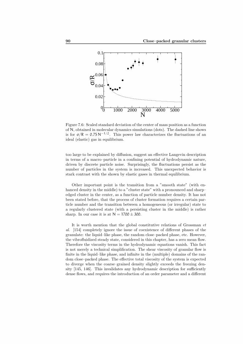
90 Close–packed granular clusters
0 1000 2000 3000 4000 5000N
0.02
0.04
0.06
0.08
0.1
0
σ/R
Figure 7.6: Scaled standard deviation of the center of mass position as a functionof N, obtained in molecular dynamics simulations (dots). The dashed line showsis for σ/R = 0.75 N−1/2 . This power law characterizes the fluctuations of anideal (elastic) gas in equilibrium.
too large to be explained by diffusion, suggest an effective Langevin descriptionin terms of a macro–particle in a confining potential of hydrodynamic nature,driven by discrete particle noise. Surprisingly, the fluctuations persist as thenumber of particles in the system is increased. This unexpected behavior isstark contrast with the shown by elastic gases in thermal equilibrium.
Other important point is the transition from a ”smooth state” (with en-hanced density in the middle) to a ”cluster state” with a pronounced and sharp–edged cluster in the center, as a function of particle number density. It has notbeen stated before, that the process of cluster formation requires a certain par-ticle number and the transition between a homogeneous (or irregular) state toa regularly clustered state (with a persisting cluster in the middle) is rathersharp. In our case it is at N = 1700 ± 300.
It is worth mention that the global constitutive relations of Grossman etal. [154] completely ignore the issue of coexistence of different phases of thegranulate: the liquid–like phase, the random close–packed phase, etc. However,the vibrofluidized steady state, considered in this chapter, has a zero mean flow.Therefore the viscosity terms in the hydrodynamic equations vanish. This factis not merely a technical simplification. The shear viscosity of granular flow isfinite in the liquid–like phase, and infinite in the (multiple) domains of the ran-dom close–packed phase. The effective total viscosity of the system is expectedto diverge when the coarse–grained density slightly exceeds the freezing den-sity [145, 146]. This invalidates any hydrodynamic description for sufficientlydense flows, and requires the introduction of an order parameter and a different
7.5 Conclusions 91
type of the stress–strain relation into the theory (cf. Ref. [153]). Luckily, thesecomplications do not appear for a zero–mean–flow state. Indeed, the equationof state, heat conductivity, and the inelastic heat loss rate do no exhibit anysingularity around the freezing point, and all the way to the hexagonal closepacking. Therefore, the hydrostatic description remains reasonably accurate farbeyond the freezing point.
Future work should focus on dense clusters (more precisely, on their “core”regions) and characterize the positional and orientational ordering at differentN. This can be achieved by measuring two correlation function: the positionalcorrelation function and the orientational correlation function. The motivationis the following. There are classical papers of Kosterlitz and Thouless, Youngand Nelson, and Halperin, from the 70-ies —these yielded the KTHNY theory ofmelting, reviewed by Strandburg in Ref. [119]—, which suggested that meltingin assemblies of elastic hard disks occurs (as the density decreases) via twocontinuous phase transition: the first one from the perfect hexagonally packedphase to the so called hexatic6 phase, and the second one from the hexatic phaseto a liquid–like phase. A main question about our inelastic system which remainto be answered is, as the density in the central region increases, whether is thereany signature of additional instabilities.
6This phase can exist between solid and liquid phases. The system in the hexatic phasehas no long-range translational order but has quasi-long-range orientational order.

92 Close–packed granular clusters

Part III
Appendices

Appendix A
Equilibrium properties of
the Lattice Gas
The driven lattice gas studied in Chapter 3 reduces to the (equilibrium) latticegas [165] for zero field. This is a model for density fluctuations and liquid-gasphase transformations. As its nonequilibrium counterpart, this is defined in asquare lattice with N = L‖L⊥ sites1. Thus, each lattice site i can exist in twostates, occupied by a particle or empty, labelled by an occupation variable ni = 1
or ni = 0, respectively. The lattice gas can be mapped to the Ising model withferromagnetic couplings 2. The Ising model is perhaps the simplest system thatundergoes a nontrivial phase transition in two or more dimensions. The modelwas initially proposed to describe ferromagnetism —the presence of spontaneousmagnetization in metals such as Fe and Ni below a critical temperature Tc—.The relation between the lattice gas and the Ising model is set by simple changeof variables, namely, si = (2ni − 1)/2, where si are spin variables capable oftwo orientations, “up” and “down”. The spin up si = 1/2 and the spin downsi = −1/2 states correspond to occupied (ni = 1) and unoccupied (ni = 0)cells, respectively. Each spin i interacts with one another via an exchangeinteraction Jij > 0. Assuming ferromagnetic coupling and isotropic interactions(Jij ≡ J > 0), the Ising Hamiltonian is
H = −J∑
〈ij〉sisj − B
N∑
i=0
si , (A.1)
where 〈ij〉 denotes neighbor interactions and B is the external magnetic field,which plays the role of the chemical potential of the lattice gas. In fact, thecanonical partition function for the ferromagnetic model is the grandcanonicalpartition function [3] for the lattice gas model. Therefore the lattice model is
1We consider here only two-dimensional lattices.2Historically, the Ising model [52] was introduced before the lattice model [165]. Likewise,
the lattice gas as and the binary alloy model [32] are equivalent.

96 Equilibrium properties of the Lattice Gas
0 0.5 1 1.5 2 2.5 3T/T
Ons
0
0.2
0.4
0.6
0.8
1
| M |
0.1 1(T
c-T)/T
Ons
1
Figure A.1: Phase transition in the Ising model with NN (circles) and NNNcouplings (squares). Left panel: Spontaneous magnetization M as a functionof the temperature. The magnetization vanishes abruptly at Tc/TOns = 1 forNN couplings, and at Tc/TOns = 2.32 for the NNN case. Otherwise is zero forT > Tc in both cases. Right panel: As expected in equilibrium systems [34] theorder parameter critical exponent do not depend on the dynamics details. Thesolid lines represent slopes of βIsing = 1/8.
isomorphic with the Ising model. Thermodynamically the descriptions of theising model and the lattice gas are equivalent, but there are simplifying featuresfor the Ising magnet. Henceforth we shall refer to them without distinction.
Lars Onsager [31, 32] gave in 1944 the (exact) partition function for thetwo-dimensional model, in the absence of external magnetic field. The On-sager solution showed the existence of a second order phase transition at Tc =
2/ln(
1 +√
2)
Jk−1B , referred to as the Onsager temperature TOns. The spon-
taneous magnetization
|M| =
∣
∣
∣
∣
∣
1
N
N∑
i=1
si
∣
∣
∣
∣
∣
(A.2)
is the order parameter for this transition. Above the critical temperature the(average) spontaneous magnetization is zero, whereas below criticality M isnon-zero, thus one finds the system in a ferromagnetic state. Due to the up-down symmetry of the Ising system, the spontaneous magnetization is doublydegenerate, with an “up” phase and a “down” phase. In the terminology of thelattice gas, there should be a dense (liquid) phase coexisting with a dilute (gas)phase below the critical temperature. Otherwise, typical configurations are dis-ordered. The left panel in Fig. A.1 shows the second order phase transition fornearest-neighbor (NN) couplings and next-nearest-neighbor (NNN) couplings,as schematized in Fig. 3.4 in Chapter 3. For NN couplings, the first sum inEq. (A.1) runs over the four NN sites, and for the NNN case it runs over theeight NNN sites. As is shown in Fig. A.1, the phase transition occurs exactlyat TOns for NN couplings. The immediate effect of considering additional neigh-

97
Figure A.2: Surface plots of the two–point correlation (upper row) and thestructure factor (lower row). These are for the Ising magnet, or equivalentlythe lattice gas, on a L‖ × L⊥ = 128 × 128 lattice with NN (left column) andNNN interactions (right column). To avoid complications due to inhomogeneousordered phases, we choose temperatures above criticality. Temperatures areT/TOns = 1.09 for the NN and T/TOns = 2.61 for the NNN case. Notice thechange of color code with each plot.
bors, as in the NNN case, is the rising of the critical temperature. For NNNcouplings, the critical temperature raises to Tc = 2.32 TOns [94]. In the neigh-borhood of the critical temperature the spontaneous magnetization behaves likeM ≈ (1 − T/Tc)
βIsing as T → Tc −. Here, βIsing is the order parameter criticalexponent. The right panel of Fig. A.1 shows the behavior of M near Tc for NNand NNN couplings. In both cases, βIsing = 1/8. This result is consistent with(equilibrium) renormalization group ideas [34], which set up that the criticalexponents are universal. It means that there are only a few parameters, suchas dimensionality and underlying symmetries which are relevant near the criti-cal point, therefore critical exponents do not depend on the particular system,either magnetic or fluid.
In zero magnetic field the pair-correlation function is of particular interestsince it in a sense measures the “degree of order” of the lattice. It is defined ingeneral from the partition function as C = 〈sisj〉, where 〈· · · 〉 (see also Eq. (3.6)in Chapter 3) denotes the proper ensemble average. Two-point correlationsare shown in Fig. A.2. Correlations in the equilibrium Ising model are shortranged, except at the critical point where the free energy shows a nonanalyticpoint, controlled by a correlation length ξ. Specifically, they decay exponen-tially (in Fig. A.2 or more clearly in Fig. A.3) when r, a typical inter-particleseparation, becomes large compared to ξ. Translated into the momentum space,

98 Equilibrium properties of the Lattice Gas
0 5 10 15 20x, y
0
0.2
0.4
0.6
0.8
1
C||, C
⊥0 2.5 5 7.5 10
nx,y
0
20
40
60
S ||, S⊥
Figure A.3: Main graph: Parallel C‖ and transverse C⊥ projections of the two–point correlation function. Symbols (parallel) and + (transverse) are for NNinteractions, whereas (parallel) and × (transverse) correspond to the NNNcase. Inset: Parallel S‖ and transverse S⊥ projections of the structure factor.Here, nx,y = 128 κx,y/2π are integers. Symbols are as in the main graph.System size and temperatures are as in Fig. A.2.
the pair correlation function lead to the structure factor S(κx, κy) (see Eq. (3.7)in Chapter 3), i.e., structure factor is the Fourier transform of the two-pointcorrelation function. Structure factors are shown in Figs. A.2 and A.3. Expo-nential decay in correlations, takes the form of “analyticity at the origin” in themomentum space. Notice also that this analyticity in the origin do not dependon whether one takes isotropic or anisotropic couplings. As indicated above, wehave assumed isotropic couplings between spins, and therefore both C and S areisotropic (more clearly in Fig. A.3). In Chapter 3 we show that the driven latticegas behaves quite differently, displaying generic power law decay in two-pointcorrelations, not only at the critical point, and discontinuity singularity at theorigin in the structure factor.
Appendix B
Interfacial stability of
Driven Lattice Gases under
saturating field
In Chapter 3 we pointed out one of the most striking, even counterintuitive,features of the Driven Lattice Gas (DLG) with nearest-neighbor (NN) inter-actions: Monte Carlo (MC) simulations with Metropolis rates show that thecritical temperature TE monotonically increases with the external driving fieldfrom the Onsager value T0 = TOns = 2.269 Jk−1
B to T∞ ' 1.4 TOns. As we con-cluded, this is associated with the fact that a driven particle is geometricallyrestrained in the DLG. In fact, allowing hops and interactions to the next-nearest-neighbors (NNN) one observes just the opposite behavior: the criticaltemperature decreases as the field increases. Moreover, there is no phase tran-sition for a large enough field, i.e., TE → 0 as E → ∞. Or in other words, inthe DLG with NNN interactions a strong field prevents transition to an orderedlow-temperature phase. This is better illustrated in Fig. 3.2 in Chapter 3. Qual-itatively, this difference of behavior in the infinite field limit between the twomodels may be understood in terms of stability of the liquid-gas interface. Thatis, in contrast with the NN case, a (well-ordered) interface cannot be stableunder a strong field in the NNN case. This suggest a balance between thermaleffects, which favor the stability (the order) of the interface [101], and drivingeffects, which would drive particles out of the interface favoring disorder.
In order to study this balance, the disparate behavior between both dy-namics, and characterize the two competing tendencies —i.e, the field vs. tem-perature balance— we propose a generalized driven lattice gas model. This isan intermediate model between the two cases above mentioned (the NN andthe NNN case) which captures the behavior in the large field limit observed ineach system. It is defined on a two-dimensional lattice L‖ × L⊥ with periodic
100 Interfacial stability of Driven Lattice Gases for E → ∞
boundary conditions in which particles interact via the usual Ising Hamiltonian,
H = −4∑
〈j,k〉σjσk . (B.1)
Each site i ∈ Z2 is either occupied by a particle or empty, which we denoteby a lattice occupation number σi taking two values: σi = 1 (occupied) orσi = 0 (empty). The sum in the Hamiltonian runs over all the NNN sites. Asin the standard DLG, dynamics is induced by the competion between a heatbath at temperature T and an external driving field E, which break the detailedbalance condition. The field is assumed pointing along one of the principal latticedirections, say horizontal. Time evolution is then by microscopic dynamicsaccording to the Metropolis transition probability per unit time w (this waspreviously defined in Eq. (3.2) in Chapter 3):
w(σ → σ′) = min
1, e(∆H+~E·~x)/kBT
. (B.2)
Here ∆H is the energy difference of a particle-hole exchange and ~E · ~x denotesthe dot product between the field and the displacement of the exchange. σ ≡σi ; i ∈ two-dimensional lattice stands for a configuration.
Given a particle, its neighboring sites along the principal lattice directionshas different probability to be reached than the sites along the diagonals (seeFig. B.1). The former are always accessible (probability 1), whereas the latterhave probability 0 ≤ α ≤ 1, parameter which is set at the beginning of thesimulation (as well as T and E). The algorithm proceed as follows1:
1. We randomly select a NNN pair i, j of sites with different occupancies,σi 6= σj.
2. As Fig. B.1 illustrates, if the selected pair is along one of the principallattice directions the exchange attempt is allowed (Go to next item). Inother case, draw a random number r1, and if r1 ≤ α then the attempt isallowed (Go to next item), otherwise rejected (Go to item 1).
3. Perform a standard MC trial move controlled by the Metropolis ratefunction w(z) = min 1, e−z, i.e., controlled by the standard biased rateEq. (B.2). To be specific, first compute z; if z ≤ 0 the attempt (particle-hole exchange) is finally accepted; if, however, x > 0, we draw a randomnumber r2 and perform the exchange only if r2 ≤ e−x.
4. Go to item 1.
Notice that when α → 0 only NN particle-hole exchanges are allowed, otherwisethere is a non-zero probability for diagonal hops. The limit case of α = 1 corre-sponds with the NNN dynamics, i.e., with the NDLG model already introduced
1The algorithm as we use it is more complicated to obtain better (and faster) results. Wedo not present this algorithm due to its complexity. Instead, we show a simpler algorithmwhich would work like this.

101
α α
αα
11
1
1
Figure B.1: Schematic diagram of the accessible sites a particle (at the center,marked with a dot) has for the αDLG. Attempts (particle-hole exchanges) alongthe principal lattice directions are always allowed (marked with probability 1).Diagonal attempts are allowed with probability α. The limit of α → 0(1)
corresponds with NN (NNN) couplings. Once α is set at the beginning, theallowed exchanges are controlled by the Metropolis rate function Eq. (B.2).
in Chapter 3. Therefore, this model (henceforth referred to as the αDLG) cancapture both the DLG and NDLG phenomenology by varying the parameter α
(the effective connectivity). One may also think on α as a temperature whichcontrols the diagonal degrees of freedom. For E = 0 this model reduces to theequilibrium lattice gas2 (see Appendix A).
We carried out extensive MC simulations on the αDLG by assuming half-filled lattices and periodic boundary conditions (toroidal conditions). Hence,nontrivial nonequilibrium steady state is set in asymptotically. As in the stan-dard DLG, MC simulations reveal that this model undergoes a temperature-induced second-order phase transition. This transition is analogous to the stud-ied in Chapters 3 and 4. However, in this appendix we are rather interestedin the stability of the interface under saturating fields. Specifically, we studythe mechanisms which lead to an ordered or disordered low-temperature statesin the large field limit, i.e., to a stable or unstable interface. To this end, werestrict ourselves to the E → ∞ limit and to T → 0. The latter limit is themost favorable case for ordering, which will enable us to identify the point inwhere the field effects outweight the thermal effects. In addition, this limit isconvenient for theoretical and computational purposes since T is no longer aparameter.
For α = 0, we observe fully frozen striped configurations, which extendsalong the field direction. Here, a one-strip liquid-like (rich-particle) phase per-colates along the field direction (the density of the vapor phase is zero). Whenincreasing α, i.e. increasing the weight of the diagonal dynamics, some particlesare driven out the interface. Nevertheless, if α is not too large, the thermaleffects still dominate. In such a case, a liquid–like (high-density) phase which isstriped then coexists with its gas (low density phase). With a further increase
2Although, of course, the equilibrium critical temperature depends on α, but not the criticalproperties. The αDLG belongs to the Ising universality class for all α.
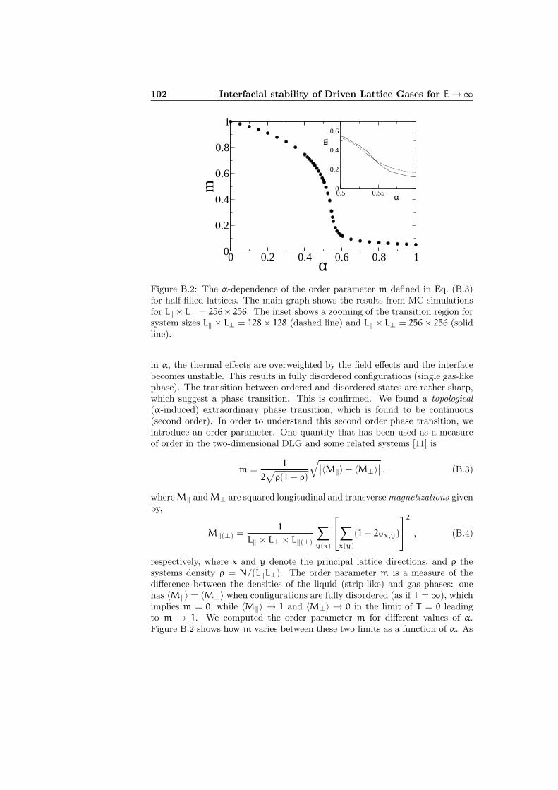
102 Interfacial stability of Driven Lattice Gases for E → ∞
0 0.2 0.4 0.6 0.8 1α0
0.2
0.4
0.6
0.8
1
m 0.5 0.55 α0
0.2
0.4
0.6
m
Figure B.2: The α-dependence of the order parameter m defined in Eq. (B.3)for half-filled lattices. The main graph shows the results from MC simulationsfor L‖ × L⊥ = 256× 256. The inset shows a zooming of the transition region forsystem sizes L‖ × L⊥ = 128 × 128 (dashed line) and L‖ × L⊥ = 256 × 256 (solidline).
in α, the thermal effects are overweighted by the field effects and the interfacebecomes unstable. This results in fully disordered configurations (single gas-likephase). The transition between ordered and disordered states are rather sharp,which suggest a phase transition. This is confirmed. We found a topological(α-induced) extraordinary phase transition, which is found to be continuous(second order). In order to understand this second order phase transition, weintroduce an order parameter. One quantity that has been used as a measureof order in the two-dimensional DLG and some related systems [11] is
m =1
2√
ρ(1 − ρ)
√
∣
∣〈M‖〉 − 〈M⊥〉∣
∣ , (B.3)
where M‖ and M⊥ are squared longitudinal and transverse magnetizations givenby,
M‖(⊥) =1
L‖ × L⊥ × L‖(⊥)
∑
y(x)
∑
x(y)
(1 − 2σx,y)
2
, (B.4)
respectively, where x and y denote the principal lattice directions, and ρ thesystems density ρ = N/(L‖L⊥). The order parameter m is a measure of thedifference between the densities of the liquid (strip-like) and gas phases: onehas 〈M‖〉 = 〈M⊥〉 when configurations are fully disordered (as if T = ∞), whichimplies m = 0, while 〈M‖〉 → 1 and 〈M⊥〉 → 0 in the limit of T = 0 leadingto m → 1. We computed the order parameter m for different values of α.Figure B.2 shows how m varies between these two limits as a function of α. As
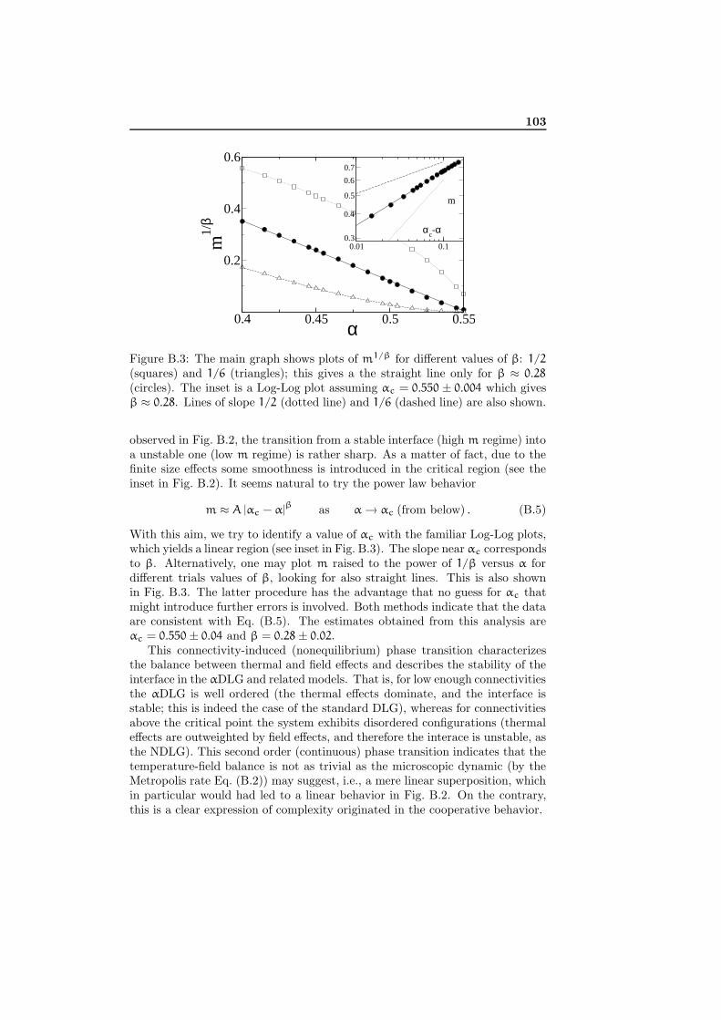
103
0.5 0.550.450.4 α
0.2
0.4
0.6
m1/
β
0.01 0.1
αc-α
0.3
0.4
0.5
0.6
0.7
m
Figure B.3: The main graph shows plots of m1/β for different values of β: 1/2
(squares) and 1/6 (triangles); this gives a the straight line only for β ≈ 0.28
(circles). The inset is a Log-Log plot assuming αc = 0.550 ± 0.004 which givesβ ≈ 0.28. Lines of slope 1/2 (dotted line) and 1/6 (dashed line) are also shown.
observed in Fig. B.2, the transition from a stable interface (high m regime) intoa unstable one (low m regime) is rather sharp. As a matter of fact, due to thefinite size effects some smoothness is introduced in the critical region (see theinset in Fig. B.2). It seems natural to try the power law behavior
m ≈ A |αc − α|β
as α → αc (from below) . (B.5)
With this aim, we try to identify a value of αc with the familiar Log-Log plots,which yields a linear region (see inset in Fig. B.3). The slope near αc correspondsto β. Alternatively, one may plot m raised to the power of 1/β versus α fordifferent trials values of β, looking for also straight lines. This is also shownin Fig. B.3. The latter procedure has the advantage that no guess for αc thatmight introduce further errors is involved. Both methods indicate that the dataare consistent with Eq. (B.5). The estimates obtained from this analysis areαc = 0.550 ± 0.04 and β = 0.28 ± 0.02.
This connectivity-induced (nonequilibrium) phase transition characterizesthe balance between thermal and field effects and describes the stability of theinterface in the αDLG and related models. That is, for low enough connectivitiesthe αDLG is well ordered (the thermal effects dominate, and the interface isstable; this is indeed the case of the standard DLG), whereas for connectivitiesabove the critical point the system exhibits disordered configurations (thermaleffects are outweighted by field effects, and therefore the interace is unstable, asthe NDLG). This second order (continuous) phase transition indicates that thetemperature-field balance is not as trivial as the microscopic dynamic (by theMetropolis rate Eq. (B.2)) may suggest, i.e., a mere linear superposition, whichin particular would had led to a linear behavior in Fig. B.2. On the contrary,this is a clear expression of complexity originated in the cooperative behavior.
104 Interfacial stability of Driven Lattice Gases for E → ∞

Appendix C
Detailed derivation of a
mesoscopic equation for the
Driven Lattice Gas with
next-nearest-neighbor
Interactions
In this appendix we detail the derivation the (mesoscopic) Langevin-type equa-tion for the Driven Lattice Gas with next-nearest-neighbor interactions (NDLG)introduced in Chapter 3. We employ and extend the method introduced inRef. [80] for the Driven Lattice Gas with nearest-neighbor couplings (DLG).
The original microscopic model consists of a two-dimensional lattice, whosesites have occupation variables σi = 1 or 0, for site i. These variables evolvefollowing a particle-hole exchange dynamics. Let us define at each point r ∈Z2 a density variable, φr ∈ R, which is the averaged value of the occupationvariables σi in a region of volume v around r. The system evolves from a givenconfiguration γ to another γ′ by choosing at random a particle at point r andexchanging it with next nearest neighbor in the µ direction at time t, namely
φ′r = φr + v−1 (δr − δr+µ) . (C.1)
When v is large enough, φr is assumed to be a continuous function of r, sayφ(r, t). This represent the coarse grained excess particle density field. So thatwe have at time t,
γ′ =φ(r) + v−1 ∇µδ(r′ − r), where φ ∈ γ
. (C.2)
We can also generalized this dynamics to consider exchanges of magnitude γ/v
106 Mesoscopic equation for the DLG with extended dynamics
with probability amplitude, the latter being an even function of η [166], e.g.,
f(η) = (δ(η + 1) + δ(η − 1)) /2 . (C.3)
Or in other words, Eq. (C.3) represents the probability distribution function ofa η, amount of mass attempted to be displaced. The configurations η evolvesaccording to a stochastic hopping dynamics which conserves the number ofparticles, or equivalently the density. That is, configurations have a statisticalweight P(γ, t), which evolves accordingly to the following continuous masterequation [1, 2]:
∂tP(γ, t) =∑
µ
∫
dηf(η)
∫
dr [Ω(γ → γ′)P(γ, t) − Ω(γ′ → γ)P(γ′, t)] , (C.4)
where Ω(γ → γ′) stands for the transition probability per unit time (transitionrate) from γ to γ′. As usual, the transition rates are given in terms of entropicand energetic contributions as
Ω(γ → γ′) = D(∆S(η)) · D(∆H(η) + Hε) . (C.5)
Here D is a function satisfying the detailed balance constraint, i.e., D(−x) =
exD(x), which ensures that in the zero field limit (ε = 0) the stationary dis-tribution is the equilibrium one, Pst ∝ e−H. ∆H and ∆S are the increment ofenergy H(γ′) − H(γ) and entropy S(γ′) − S(γ), respectively. At a mesoscopiclevel, the equivalent to the microscopic Hamiltonian (Eq. (3.1) in Chapter 3)is the standard φ4 (Ginzburg–Landau) Hamiltonian. The structure of the freeenergy consist of two contributions [33]: entropic and energetic which are givenby, respectively
S(γ) = v
∫
dr(a
2φ2 +
g
4!φ4
)
H(γ) = v
∫
dr
(
1
2(∇φ)
2+
τ
2
)
, (C.6)
where a and g are entropic coefficients whereas the parameter τ comes fromthe energetic functional. Notice that, in Eq. (C.5) the increment of energyfrom the drive Hε enters the dynamics though D(∆H(η) + Hε), where Hε =
η µ · ε (1 − φ2) + O(v−1). This means that the transition rates depend on theenergy and entropy difference between configurations plus a term Hε whosedominant part in v−1 is the natural choice to mirror the effects of the driveas far as it accounts for the local increment of energy due to the driving field.Notice also that the detailed dependence of the coarse–grained field ε on themicroscopic field introduced in Eq. (3.2) remain still as an open issue [11]. Wealso assumed the driving field acting along one of the principal lattice directions,say horizontal.
107
The next step is to get a Fokker-Planck equation by expanding the masterequation Eq. (C.4) in v−1 up to v2 order (Kramers–Moyal expansion [1]). Tothis end, we expand a functional F around γ which read,
F(γ′) = F(γ) +
∞∑
k=1
−ηkv−k
k!
(
∇µ
δ
δφ
)k
F(γ) , (C.7)
where F is a functional representing either S, H, or P. The operator δδφ
means
the functional derivative of F(φ) with respect to φ. To be specific, we alsochoose Hε as
Hε(γ′ → γ′) = ηλ(ε)µ +
∞∑
k=1
(−1)kηk+1v−k
(k + 1)!
(
∇µ
δ
δφ
)k
λ(ε)µ , (C.8)
with λ(ε)µ = µ·ε
(
1 − φ(r)2)
. These expansions yield the following Fokker-Planckequation [80].
∂tPt =∑
µ
∫
dr
(
∇µ
δ
δφ
)
×[
v−1p(λSµ, λH
µ + λεµ)Pt +
1
2v2q(λS
µ, λHµ + λε
µ)
(
∇µ
δ
δφ
)
Pt
]
, (C.9)
where
Pt ≡ P(γ, t),
λXµ ≡ −
(
∇µ
δ
δφ
)
X,
p(z1, z2) ≡∫
dη η f(η) D(ηz1) D(ηz2),
q(z1, z2) ≡∫
dη η2 f(η) D(ηz1) D(ηz2). (C.10)
After using standard techniques in the theory of stochastic processes [1] wederive from the Fokker–Planck equation its stochastically equivalent Langevinequation using the Ito prescription, which reads
∂tφ(r, t) =∑
µ
∇µ
[
p(λSµ, λH
µ + λεµ) + q(λS
µ, λHµ + λε
µ)1/2 ξµ(r, t)]
. (C.11)
The time has been rescaled by v−1 and ξµ(r, t) is a delta-correlated Gaussianwhite noise, i.e., 〈ξµ(r, t)〉t = 0 and 〈ξµ(r, t) ξµ′(r′, t′)〉 = δµµ′δ(t− t′)δ(r− r′).
We focus on the critical region where large fluctuations on all length scalesdominate. Further simplification in Eq. (C.11) is possible in this regime bydropping the irrelevant terms in the renormalization group sense. Following the
108 Mesoscopic equation for the DLG with extended dynamics
standard field theoretic methods let us introduce an external momentum scaleτ and make the following anisotropic scale transformations
t → τ−zt ,
r⊥ → τ−1r⊥ ,
r‖ → τ−sr‖ ,
φ → τδφ .
(C.12)
Next, we expand the Langevin equation in powers of τ around τ = 0, keap-ing only the leading terms. For next-nearest-neighbor interactions, the sum
∑µ
involves a sum for each possible direction, namely∑
‖∑
⊥∑
∑ which are re-
spectively the parallel, transverse, and the two diagonals directions. After somecumbersome algebra, one can split the terms depending on both diagonal (and ) into the two parallel and transversal to the driving field ε components.The time scale, the transverse noise, and the transverse spatial interaction areforced to remain invariant under transformation. With this, one gets z = 4 andδ = (s+d−3)/2. Different scenarios are now possible depending on the value ofs. Demanding that the most relevant terms in the parallel and transverse to thefield scale in the same way, as in the standard analysis of the critical behaviorof the NDLG (see subsection 3.3.2), would lead to s = 2. According to this,the Langevin equation for finite (coarse–grained) driving field contains a largebunch of ε-dependent terms. Similarly to what occurs in Ref. [80], just takinga large enough value of the driving field most of those terms vanish. By doingthis, one is led to the following Langevin equation
∂tφ(r, t) = −∇4⊥φ + (τ +
3
2a)∇2
⊥φ +g
4∇2
⊥φ3 + a∇2‖φ + ξ(r, t) (C.13)
The resulting Langevin equation is analogous to the one for nearest-neighbor in-teractions (see Eq. (3.10) in Chapter 3), although Eq. (C.13) contains additionalentropic, not energetic, contributions due to the presence of larger number ofbonds than in the NN case.
Appendix D
Hydrodynamic description
for a three-dimensional
granular gas: Clustering
and symmetry breaking
A straightforward extension to three dimensions of the circular system studiedin Chapter 7 is a cylinder in which the curved wall is maintained at a constanttemperature and the other two are elastic (see Fig. D.1). Particles of diameter d
move inside the cylinder underging inelastic collisions with a constant restitutioncoefficient µ. In this appendix we study the clustering and symmetry-breakinginstabilities employing granular hydrodynamics in such a geometry. To thisend, we generalize the Grossman et al. [154] constitutive relations to three-dimensional situations.
Constitutive Relations. Before go further, we derive heuristic constitutiverelations for inelastic gases in three dimensions employing free volume argumentsin the vicinity of the close packing, and suggest an interpolation between theclose-packing limit and the usual dilute-limit relations. We follow here thestrategy taken by Grossman et al. [154] in two dimensions.
Let us consider our three-dimensional system, in which there is a temper-ature gradient in the radial direction because of the thermalized wall (set attemperature T0). As a result, there will be an energy flux along this direction.Consequently —assuming both azimuthal and longitudinal symmetry, i.e, thestate do not depend neither θ nor x—, the energy balance equation, which isderived from the hydrostatic version of Eqs. (5.1), reduces to
1
r
d
dr
(
rκdT
dr
)
= I , (D.1)
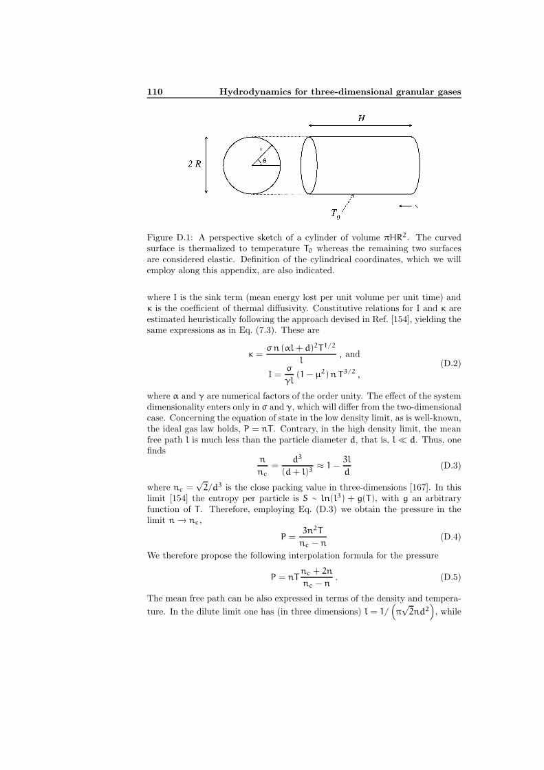
110 Hydrodynamics for three-dimensional granular gases
Figure D.1: A perspective sketch of a cylinder of volume πHR2. The curvedsurface is thermalized to temperature T0 whereas the remaining two surfacesare considered elastic. Definition of the cylindrical coordinates, which we willemploy along this appendix, are also indicated.
where I is the sink term (mean energy lost per unit volume per unit time) andκ is the coefficient of thermal diffusivity. Constitutive relations for I and κ areestimated heuristically following the approach devised in Ref. [154], yielding thesame expressions as in Eq. (7.3). These are
κ =σ n (αl + d)2T1/2
l, and
I =σ
γl(1 − µ2) n T3/2 ,
(D.2)
where α and γ are numerical factors of the order unity. The effect of the systemdimensionality enters only in σ and γ, which will differ from the two-dimensionalcase. Concerning the equation of state in the low density limit, as is well-known,the ideal gas law holds, P = nT . Contrary, in the high density limit, the meanfree path l is much less than the particle diameter d, that is, l d. Thus, onefinds
n
nc
=d3
(d + l)3≈ 1 −
3l
d(D.3)
where nc =√
2/d3 is the close packing value in three-dimensions [167]. In thislimit [154] the entropy per particle is S ∼ ln(l3) + g(T), with g an arbitraryfunction of T . Therefore, employing Eq. (D.3) we obtain the pressure in thelimit n → nc,
P =3n2T
nc − n(D.4)
We therefore propose the following interpolation formula for the pressure
P = nTnc + 2n
nc − n. (D.5)
The mean free path can be also expressed in terms of the density and tempera-
ture. In the dilute limit one has (in three dimensions) l = 1/(
π√
2nd2)
, while
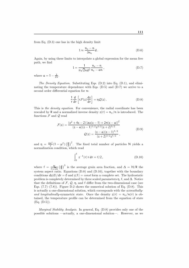
111
from Eq. (D.3) one has in the high density limit
l ≈ nc − n
3nc
d . (D.6)
Again, by using these limits to interpolate a global expression for the mean freepath, we find
l =1
π√
2nd2
nc − n
nc − an, (D.7)
where a = 1 − 32π
.
The Density Equation. Substituting Eqs. (D.2) into Eq. (D.1), and elimi-nating the temperature dependence with Eqs. (D.5) and (D.7) we arrive to asecond order differential equation for n:
1
r
d
dr
[
rF(z)dz
dr
]
= ηQ(z) . (D.8)
This is the density equation. For convenience, the radial coordinate has beenrescaled by R and a normalized inverse density z(r) = nc/n is introduced. Thefunctions F and Q read
F(z) =(z2 + 4z − 2) [αz(z − 1) + 2π(z − a)]
2
(z − a)(z − 1)1/2z3/2(z + 2)5/2
Q(z) =(z − a)(z − 1)1/2
(z + 2)3/2z1/2,
(D.9)
and η = 4π2
γ(1 − µ2)
(
Rd
)2. The fixed total number of particles N yields a
normalization condition, which read
∫1
0
z−1(r) r dr = f/2 , (D.10)
where f = N
π√
2∆
(
dR
)3is the average grain area fraction, and ∆ = H/R the
system aspect ratio. Equations (D.8) and (D.10), together with the boundaryconditions dz(0)/dr = 0 and z(1) = const form a complete set. The hydrostaticproblem is completely determined by three scaled parameters η, f, and ∆. Noticethat the definitions of F , Q, η, and f differ from the two-dimensional case (seeEqs. (7.7)–(7.8)). Figure D.2 shows the numerical solution of Eq. (D.8). Thisis actually a one-dimensional solution, which corresponds with the azimuthally-and longitudinally-symmetric state. Once the density z(r) = nc/n(r) is ob-tained, the temperature profile can be determined from the equation of state(Eq. (D.5)).
Marginal Stability Analysis. In general, Eq. (D.8) provides only one of thepossible solutions —actually, a one-dimensional solution—. However, as we
112 Hydrodynamics for three-dimensional granular gases
0 0.2 0.4 0.6 0.8 10
0.2
0.4
0.6
0.8
1
T/T
0
n/n c
Figure D.2: Scaled temperature (dashed line) and density (solid line) profilespredicted by the hydrostatic theory for η = 104 and f = 0.036.
will demonstrate, this system exhibits symmetry-breaking instability1. That is,there are truly two-dimensional solutions in which the longitudinal symmetryalong x is broken. These solutions can be found by linearizing Eq. (D.8) aroundthe one-dimensional solution given by Eqs. (D.8)–(D.10) —a similar analysiswas performed in Chapters 6 and 7—. In general, one can rewrite the energybalance equation in terms of the three coordinates r, θ, and x:
∇ · (F(r)∇z) = ηQ(z) , (D.11)
with F and Q given by Eq. (D.9). Substituting z(r, θ, x) ∼ z(r) + εω(r, θ, x),assuming ω = Ξ(r)Π(θ)Φ(x), and linearizing Eq. (D.11) with respect to thesmall correction ε, one obtains:
Φ(x) = A sin(mx) + B cos(mx) , x ∈ [0, ∆]
Π(θ) = C sin(kθ) + D cos(kθ) , θ ∈ [0, 2π)
Γ ′′ +1
rΓ ′ −
(
m2 +k2
r+
ηQ′
F
)
Γ = 0 , r ∈ [0, 1] ,
(D.12)
where A,B C, and D are constants, and m and k are, respectively, the longitudi-nal and azimuthal wave number determined by the boundary conditions. Here,Γ(r) ≡ Ξ(r)F , Q′ denotes the z derivative of Q, and functions F and Q areevaluated at z = z(r). For fixed values of η and f, Eq. (D.12) and the boundaryconditions
Φ′(0) = Φ′(∆) = 0 (D.13)
represent a linear eigenvalue problem for k and m. We focus here only inthe longitudinal wave number m, so that m = jπ/∆, where j ∈ 0, N be-cause of the boundary conditions Eq. (D.13). That is, we solve numericallythe eigenvalue problem for k = 0. If there are nontrivial solutions for the low-est mode k = 0 then there will be solutions for higher modes. Moreover, in
1This is in contrast with its two-dimensional counterpart, previously studied in Chapter 7.

113
3 3.5 4 4.5 5
f × 1030
1
2
3
4
m
0 0.2 0.4 0.6 0.8r
0
0.5
1
1.5
2
Γ m
stable
unstable
Figure D.3: Main graph: Marginal stability curve m = m(f) for η = 105.The symmetry-breaking instability develops in the parameter region above thiscurve. Inset: Eigenfunction Γm(r) corresponding to the eigenvalue m = 0.585
for η = 105 and f = 2.16 · 10−3.
Chapter 7 we proved the stability of the azimuthally-symmetric state —againstlinear perturbations—, hence one expects that the azimuthal wave number k
does not play a relevant role here. The symmetry breaking instability alongthe longitudinal (not azimuthal) direction is confirmed. Figure D.3 shows themarginal stability curve m = m(f) found numerically. For a fixed value of η theazimuthally- and longitudinally-symmetric state is unstable (stable) for any m
below (above) the marginal stability curve. Interestingly, the symmetric stateremains stable for any m beyond a finite interval of f ∈ (fmin, fmax). Or inother words, for each aspect ratio ∆ > ∆crit = πj/m, where j = 0, 1, 2, . . ., thesymmetric state loses stability with respect the longitudinal mode j [159].
Therefore, granular hydrodynamics, employing our heuristic constitutive re-lations —an extension of the Grossman et al. approach to three-dimensionalcases—, may be a good candidate to describe the clustering and symmetry-breaking instabilities which may occur in inelastic hard-sphere systems.
114 Hydrodynamics for three-dimensional granular gases

Part IV
Conclusions

Conclusions and future
work
Unfortunately, despite of the much research efforts, a rigorous statistical-mechan-ical description of nonequilibrium instabilities remains still elusive. The workpresented here goes deep into the nonequilibrium realm, aiming for a new efforttowards better understanding basic features of nonequilibrium phase transitions.Indeed, the study of driven diffusive fluids and driven granular gases, besidesits technological importance, is of general interest because it will contribute tothe rationalization of nonequilibrium phenomena. The emphasis in our investi-gations is on the study —in most cases at different levels of description, namely,macroscopic, mesoscopic, and microscopic— of the instabilities which occur inthose systems. This task were carried out with both state-of-the-art and noveltheoretical and computational techniques in statistical physics.
This thesis was structured in four parts. The first part, which comprisesChapters 2, 3, and 4, was devoted to the early–time kinetic and steady stateproperties of driven diffusive fluids ; the Part II (Chapters 5, 6, and 7) dealtwith both the atomistic and macroscopic description of two-dimensional driveninelastic gases; finally, Appendices A, B, C, and D were enclosed in Part III.In what follows (Part IV), we summarize the main results and the original con-tributions contained in this work. We also give an outlook for principal issuesto be investigated in future work.
Chapter 1. In the first chapter we reviewed the general features, phenomenol-ogy, and open issues of the class of systems which we are dealing with in the textfrom a mechanical-statistical point of view. Likewise we remarked the subjectof this thesis as well as the main motivation behind it.
Chapter 2. In this chapter we presented the model —i.e., the driven latticegas (DLG)— which was the prototype for driven diffusive fluids, and sum-marized some of its already known, unusual properties and controversies. Therelevant background for Chapters 3 and 4 is also provided. This comprises state-of-the-art simulation schemes (lattice and off-lattice Metropolis Monte Carlo)as well as field–theoretical approaches (statistical field theories).

118 Conclusions and future work
Chapter 3. We have described Monte Carlo simulations and field theoret-ical calculations that aim at illustrating how slight modifications of dynamicsat the microscopic level may influence, even quantitatively, both the resultingnonequilibrium steady state and the kinetic properties. With this aim, we tookas a reference the DLG. We introduced related lattice and off-lattice microscopicmodels in which particles, as in the DLG, interact via a local anisotropic rule.The rule induces preferential hopping along one direction, so that a net currentsets in if allowed by boundary conditions. In particular, we have discussed onthe similarities and differences between the DLG and its continuous counterpart,namely, a Lennard–Jones analogue in which the particles’ coordinates vary con-tinuously. A comparison between the two models allowed us to discuss someexceptional, hardly realistic features of the original discrete system —which hasbeen considered a prototype for nonequilibrium anisotropic phase transitions(although we claim here is not justified). We outline the main conclusions asfollows:
• We found that the continuous, off-lattice model closely resembles the DLGin that both depict a particle current, a highly anisotropic liquid-vaporinterface which extends along the field direction, and the correspondingsecond order phase transition.
• However, they differ in some essential features. Contrary to the DLG,its off-lattice counterpart shows a transition temperature which decreaseswith the field strength. Moreover, unlike for the DLG, there is no phasetransition for a large enough field. Concerning the early process of kineticordering, early–time anisotropies in the off–lattice case point along thefield, contrary to the ones observed in the discrete DLG.
• These observations suggest that the DLG behavior is highly conditioned bythe lattice geometry, which acts more efficiently in the DLG as an orderingagent than the field itself. Therefore, the striking, counterintuitive featureof the DLG that a strong field raises the critical temperature above theequilibrium one is a geometrical effect —induced by the lattice topology—rather than dynamic.
• In particular, it ensues that, due to its uniqueness, the DLG does not havea simple off-lattice analog.
• In order to deepen in this situation, we studied the DLG with an infi-nite drive extending hops and interaction to next–nearest–neighbors (thismodel was named NDLG). We confirmed that the NDLG behaves closerto the off-lattice case: the critical temperature decreases with the fieldand early–time anisotropies point along the field.
• However, we found that allowing jumping along intermediate directionsleaves invariant both spatial correlations and criticality. The former was
119
monitorized by the two-point correlation function and the equal-time struc-ture factor, whereas the latter was determined by standard finite sizescaling, and corroborated by the anisotropic driven system (ADS) (meso-scopic) approach.
• Therefore, allowing jumping along intermediate directions modifies essen-tially the phase diagram —which is not determined by bare symmetryarguments— but not features (such as generic power–laws in spatial cor-relations) that seem intrinsic of the nonequilibrium nature of the phe-nomenon.
These conclusions are properly complemented by the results obtained in theChapter 4 on criticality in a related off-lattice model. Moreover, we believe thatthe fact that particles are constrained to travel along discrete lattice directionsmay condition not only the DLG’s properties, but also the properties of manyother lattice models. Further research, which is going on at present, confirmsthis on the off-lattice versions of the Time Asymmetric Exclusion Process [16, 57](TASEP), and of the DLG with nearest neighbor repulsion [91, 93]. Further is-sues are the characterization of the stability of the interface under strong fields(see Appendix B), and the study of the early–time kinetic of phase separationin the NDLG from the field–theoretical point of view, by using the successfulADS approach.
Chapter 4. Since the DLG was shown in Chapter 3 to be unrealistic insome essential sense, we introduced here a novel, realistic off–lattice drivenfluid, which is a candidate to portray some of the anisotropic behavior in na-ture. This is a nonequilibrium Lennard-Jones fluid with an external constantdriving field, settled on a thermal bath. We studied short–time kinetic andsteady–state properties of its non–equilibrium phases, namely, solid (mono- andpolycrystalline), liquid and gas anisotropic phases. Specifically, we describedthe early–time segregation process as monitored by the excess energy, whichmeasures the droplets surface; structural properties of the steady state, namely,the radial and azimuthal distribution functions, and the degree of anisotropy;transport properties; and also an accurate estimate of the liquid–vapor coexis-tence curve and the associated critical indeces. The principal conclusions are:
• This model seems to contain the necessary essential physics to be usefulas a prototypical model for anisotropic behavior in nature.
• This case is more convenient for computational purposes, than others suchas, for instance, standard molecular–dynamics realizations of driven fluidsystems.
• This is the natural extension to nonequilibrium anisotropic cases of the fa-miliar Lennard-Jones fluid, which has played an important role in analysingequilibrium fluids. Indeed, our model reduces to the (equilibrium) Lennard-Jones fluid for zero field. Otherwise, it exhibits a net current, and stripedstructures below a critical point.
120 Conclusions and future work
• Concerning kinetics properties, in spite of the anisotropy of the late–time“spinodal decomposition” process, earlier nucleation seems to proceed bySmoluchowski coagulation and Ostwald ripening, which are known to ac-count for nucleation in equilibrium, isotropic lattice systems and actualfluids.
• Unexpectedly, we have also found that the model critical behavior is con-sistent with the Ising, equilibrium one but not with the one for the DLG.The main reason for this and other disagreements discussed in this chap-ter might be the particle–hole symmetry violation in the driven Lennard–Jones fluid.
• In addition, regarding the modeling of complex systems, one may infer thatspatial discretization may change significantly not only morphological andearly–time kinetics properties, but also critical properties. This is in starkcontrast with the concept of universality in equilibrium systems, wherecritical properties are independent of dynamic details.
• Finally, we believe this model will motivate new experiments on anisotropicspinodal decomposition besides theoretical work. In fact, our observa-tions on the early-time separation process and structural properties areeasily accessible by micro calorimetric and spectroscopy experiments, forinstance.
Many other issues remain. Further research, which are going on at this mo-ment, involve detailed studies of its interfacial properties, the role of the finitesize effects, and sheared versions of this driven Lennard–Jones fluid. Otherquestions which we would like to raise for future work is how do the particle-hole symmetry and the shape of the interaction potential influence the criticalproperties. A detailed analysis of the late–time segregation process, which hasalready been studied for both equilibrium [107, 108] and non–equilibrium cases,including the DLG [103, 109], will be the subject of future investigations. Alsointeresting is the detailed study of the structure and morphological features ofthe (monocrystalline) solid and glass–like (polycrystalline solid) phases. Thefact that our off-lattice model and a related driven-diffusive model [91] exhibita critical behavior consistent with Ising is rather remarkable, and merits furtherinvestigations.
Chapter 5. In this chapter we have provided the framework relevant to Chap-ters 6 and 7. We discussed on some unresolved puzzles and recent developmentsin granular fluids, in particular, on the applicability of granular hydrodynamicsto granular flows. We also presented the basic ingredients of the studied modelsand the computer simulation methods (event-driven molecular dynamics).
Chapter 6. We have described hydrodynamic derivations as well as event-driven molecular dynamics simulations in a monodisperse granular gas confinedin an annulus, the inner circle of which represents a “thermal wall”. The quasi-elastic limit was considered, and the granular hydrodynamics with Enskog-type
121
transport coefficients [135] was employed. We performed a comprehensive studyof the clustering, symmetry breaking and phase separation instabilities, whichenable us to stablish a detailed phase diagram. To test and complement ourtheoretical predictions we performed event-driven molecular dynamics simula-tions of this system. This led us to discuss on the physics of the instabilitieswhich occur in this model. Here we itemize the main conclusions:
• The zero-flow regime was completely determined by three scaled param-eters: the grain area fraction, the inelastic heat loss parameter, and theaspect ratio of the annulus.
• In our event-driven molecular dynamics simulations, azimuthally symmet-ric steady states were observed far from the driving wall. In spite of thesmall number of particles employed, these annular states were accuratelydescribed by the numerical solutions of our granular hydrostatic equations.
• A marginal stability analysis yielded a region of the (three-dimensional)parameter space where the annular state —the basic, azimuthally sym-metric steady state of the system— is unstable with respect to smallperturbations which break the azimuthal symmetry. We computed themarginal stability curves and compared them to the borders of the spin-odal (negative compressibility) interval of the system.
• We found that, the physical mechanism of the phase separation insta-bility is the negative compressibility of the granular gas in the azimuthaldirection, caused by the inelastic energy loss. Mathematically, phase sepa-ration manifests itself in the existence of additional solutions to the densityequation in some region of the parameter space.
• Our event-driven simulations of this system also showed phase separation,but it is masked by large spatio-temporal fluctuations. By measuring theprobability distribution of the amplitude of the fundamental Fourier modeof the azimuthal spectrum of the particle density we were able to clearlyidentify the transition to phase separated states in the simulations.
• We found that the instability region of the parameter space, predictedfrom hydrostatics, is located within the phase separation region observedin our simulations. This implies the presence of a binodal (coexistence)region, where the annular state is metastable.
• Clustering, symmetry breaking, and phase separation instabilities shouldbe observable in actual experiments. In fact, the model we proposed isexperimentally accessible, and, therefore, if brought to the attention ofthe appropriate community, might stimulate experimental work on theseinstabilities.
Of course, it would be interesting to test the predictions of our theory/simulationsin experiment. By focusing on the annular geometry, we hope to motivate ex-perimental studies of these granular instabilities which may be advantageous

122 Conclusions and future work
in this geometry. The annular setting avoids lateral side walls (with an un-necessary/unaccounted for energy loss of the particles). A possible experimentcan employ metallic spheres rolling on a slightly concave smooth surface anddriven by a rapidly vibrating (slightly eccentric and possibly rough) interiorcircle. While particle rotation and rolling friction may become important, weexpect that the main predictions of the theory will persist. It would be also in-teresting to determine the nature (sub- or supercritical?) of the solutions whichbifurcate from the azimuthally symmetric state. Further studies may exploitthe similarities between the phenomenology observed in our model system andthe one in planetary rings, in which clustering, spontaneous symmetry breaking,oscillations, and many other instabilities occur.
Chapter 7. In this chapter we addressed granular hydrodynamics and fluc-tuations in a simple two–dimensional granular system under conditions whenfirst-principle hydrodynamic descriptions break down because of large density,not large inelasticity. We put it into a test —using event-driven moleculardynamics simulations— in an extreme case when granular clusters with themaximum density close to the hexagonal close packing form (we defined themas macro–particles). The model system we considered here, comprises inelasti-cally colliding hard disks enclosed by circular boundaries, driven by a thermalwall at zero gravity. The main conclusions are summarized as follows:
• Molecular dynamics simulations showed a sharp–edged close–packed clus-ter (macroparticle) of an almost circular shape, weakly fluctuating in spaceand isolated from the thermal wall by a low-density gas. This is due tocollisional cooling. The macroparticle formation requires a certain numberof particles, and, as the particle density is increased, the transition froma (quasi-) homogeneous state to a macroparticle is rather sharp.
• We were able to solve numerically a set of granular hydrostatic equationswhich employ the constitutive relations by Grossman et al. [154]. Wefound that the density profiles, in a wide range of parameters, agrees al-most perfectly —including the close-packed part— with the azimuthallysymmetric solution of granular hydrostatic equations. We also showedthat, for the same setting, first-principle Enskog-type relations [135] per-form poorly.
• This agrees with previous results in rectangular geometry, with and with-out gravity, and extends the validity of the Grossman et al. relations fora slightly lower restitution coefficient, and for the circular geometry.
• A marginal stability analysis have shown —independently of the consti-tutive relations employed— that there are no steady–state solutions withbroken azimuthal symmetry which would bifurcate from the azimuthallysymmetric solution. This agrees with the persistence of circular shapesfor the macroparticle as observed in our simulations.
123
• We addressed, for the first time, fluctuations of the macroparticles, bymeasuring the radial probability distribution function of the center of massof the system. These fluctuations turn out to be Gaussian.
• The observed Gaussian fluctuations of the center of mass suggest an ef-fective Langevin description in terms of a macroparticle in a confiningpotential of hydrodynamic nature, driven by discrete particle noise —i.e.,the cluster performs a Brownian motion inside the system. The associatedLangevin equation is provided.
• In stark contrast with equilibrium systems, in which the relative magni-tude of fluctuations decreases with increasing the number of particles2, wefound that the fluctuations persist as the number of particle in the systemis increased.
There are still many open issues. A question that should be addressed is whetherare there additional instabilities in this model system. For instance, an im-portant insight, in analogy with the KTHNY theory [119] of two-dimensionalmelting (for fluids at thermal equilibrium), might be given by the positional andorientational ordering of the macroparticles at different number densities. Thiscan be achieved by measuring their respective correlation functions. In addition,both a general solution of the time-dependent hydrodynamic equations and anon-linear stability analysis will contribute to the quest. Other future issue mayinvolve the detailed study of instabilities in related three-dimensional systems.An outline can be found in Appendix D. It should be also worthy to study howpolydisperse granulates behave in this system.
In spite of appendices are commonly pushed into the background, we thinkthat our Appendices B and D merit their own conclusions.
Appendix B. In this appendix we introduced a driven-diffusive lattice model(the αDLG) which aim at understanding the balance between thermal and fieldeffects which take place in such a models, as the DLG and related models(specifically the models studied in Chapter 3). This balance can be understoodin terms of stability of the interface between the condensed and vapor phases—which are elongated along the field direction—. Thermal effects favor thestability (the order) of the interface, whereas the driving effects would driveparticles out of the interface favoring disorder. We studied this dynamic balancein the extreme case of saturating field, zero temperature limit. The main resultsare:
• Our model undergoes a second-order phase transition employing as orderparameter the measure of the ordering on the lattice as a function of theeffective connectivity. That is, for low enough connectivities the systemis well ordered (the thermal effects dominate, and the interface is stable),
2For an ideal gas in equilibrium: σ ∼ O(N−1/2), where σ is the relative magnitude offluctuations and N is the number of particles.

124 Conclusions and future work
whereas for connectivities above the critical point αc the system exhibitsdisordered configurations (thermal effects are outweighted by field effects,and therefore the interace is unstable).
• We computed the critical indexes associated with the transition.
• This second order (continuous) phase transition indicates that the tempera-ture-field balance is not as trivial as the microscopic dynamic may suggest,i.e., a mere linear superposition [54]. On the contrary, this is a clear ex-pression of complexity originated in the cooperative behavior.
Appendix D. The last appendix addressed clustering and symmetry-breakinginstabilities in a monodisperse gas of inelastic hard spheres confined in a cylin-der, the curved wall of which represents a “thermal wall”. We employed a setof granular hydrodynamic equations with heuristic constitutive relations, whichwe derived from free-volumen arguments. This model is a simple extension forthree-dimensional cases of the circular system studied in Chapter 7.
• Following the Grossman et al. [154] strategy, we proposed phenomeno-logical expressions for the equation of state and the transport coefficientsfor three-dimensional cases. We employed free-volume arguments in thevicinity of the close packing, and suggested an interpolation between thehexagonal-packing limit and the well-known low density relations.
• The stationary solutions of the granular hydrodynamic equations predictsymmetric clustered states far from the thermal wall. Some of the solu-tions bifurcate from the (steady-state) symmetric solution, i.e., hydrody-namic also predicts the existence of broken-symmetry states. The pres-ence of symmetry breaking instability in this system is in contrast withour findings in its two-dimensional counterpart (see Chapter 7) in whichno symmetry breaking instability was found.
• Granular hydrodynamics, employing our heuristic constitutive relationsmay be a good candidate to describe the clustering and symmetry-breakinginstabilities which may occur in inelastic hard-sphere systems.
Published work
• Manuel Dıez-Minguito, Pedro L. Garrido, and Joaquın Marro, Lennard-Jones and lattice models of driven fluids, Phys. Rev. E 72, 026103 (2005).
• Joaquın Marro, Pedro L. Garrido, and Manuel Dıez-Minguito, Nonequili-brium anisotropic phases, nucleation and critical behavior in a drivenLennard-Jones fluid, Phys. Rev. B 73, 184115 (2006).
• Manuel Dıez-Minguito, Pedro L. Garrido, and Joaquın Marro, Lattice ver-sus Lennard-Jones models with a net particle flow in Traffic and GranularFlows ’05, in press (Springer, Berlin, 2006).
• Baruch Meerson, Manuel Dıez-Minguito, Thomas Schwager, and ThorstenPoschel, Close-packed granular clusters: hydrostatics and persistent Gaus-sian fluctuations, submitted to Europhys. Lett. (2006)
• Manuel Dıez-Minguito, J. Marro, and P. L. Garrido, On the similari-ties and differences between lattice and off-lattice models of driven fluidsin Workshop on Complex Systems: New Trends and Expectations, to bepublished in Euro. Phys. J.-Special Topics (2006).
• Manuel Dıez-Minguito and Baruch Meerson, Phase separation of a drivengranular gas in annular geometry, submitted to Phys. Rev. E (2006).
ABSTRACTS
• Manuel Dıez-Minguito, Pedro L. Garrido, Joaquın Marro, and Franciscode los Santos, Driven two-dimensional Lennard-Jones fluid in ModelingCooperative Behavior in the Social Sciences, P. L. Garrido, J. Marro, M.A. Munoz (eds.), AIP Conference Proceedings 779, 199 (2005).
• Manuel Dıez-Minguito, Pedro L. Garrido, Joaquın Marro, and Franciscode los Santos, Simple computational Lennard-Jones fluid driven out-of-equilibrium, in XIII Congreso de Fısica Estadıstica FISES’05, AbstractBook (2005).
• Manuel Dıez-Minguito and Baruch Meerson, Phase separation of a drivengranular gas in annular geometry, in XIV Congreso de Fısica EstadısticaFISES’06, Abstract Book (2006).
126 Published work
IN PREPARATION
• Manuel Dıez-Minguito, A. Achahbar, Pedro L. Garrido, and Joaquın Marro,Langevin-type description for the driven lattice gas with next-nearest-neighbordynamics (2006).
• Manuel Dıez-Minguito and Thorsten Poeschel, On the validity of globalequations of state for driven granular gases (2006).
• Manuel Dıez-Minguito, Pedro L. Garrido, and Joaquın Marro, Interfacialproperties in a nonequilibrium microfluidic system (2006).
The author acknowledge financial support from the Spanish Ministry forScience (MEC) and FEDER (project FIS2005-00791).
Bibliography
[1] N. G. van Kampen, Stochastic Processes in Chemistry and Physics, (NorthHolland, Amsterdam, The Netherlands, 1981).
[2] C. W. Gardiner, Handbook of Stochastic Methods for Physics, Chemistryand the Natural Sciences, (Springer, Berlin, Germany, 2004).
[3] R. Balescu, Equilibrium and Nonequilibrium Statistical Mechanics, (JohnWiley & Sons, New York, U.S.A., 1975); K. Huang, Statistical Mechanics,(John Wiley & Sons, New York, U.S.A., 1987).
[4] J. Biel, Formalismo y Metodos de la Termodinamica, (Editiorial Reverte,Barcelona, Spain, 1998).
[5] O. Lioubashevski, Y. Hamiel, A. Agnon, Z. Reches and J. Fineberg, Os-cillons and propagating solitary waves in a vertically vibrated colloidalsuspension, Phys. Rev. Lett. 83, 3190 (1999).
[6] N. Goldenfeld and L. P. Kadanoff, Simple lessons from complexity, Science284, 87 (1999).
[7] M. C. Cross and P. C. Hohenberg, Pattern formation outside of equilib-rium, Rev. Mod. Phys. 65, 851 (1993).
[8] J. P. Gollub and J. S. Langer, Pattern formation in nonequilibriumphysics, Rev. Mod. Phys. 71, S396 (1999).
[9] A.-L. Barabasi and H. E. Stanley, Fractals Concepts in Surface Growth,(Cambridge University Press, Cambridge, U.K., 1995).
[10] P. Bak, How Nature Works: The Science of Self-Organised Criticality,(Copernicus, New York, U.S.A., 1996).
[11] J. Marro and R. Dickman, Nonequilibrium Phase Transitions in LatticeModels, (Cambridge University Press, Cambridge, U.K., 1999).
[12] H. Haken, Cooperative phenomena in systems far from thermal equilibriumand in nonphysical systems, Rev. Mod. Phys. 47, 67 (1975).

128 BIBLIOGRAPHY
[13] Far from Equilibrium Phase Transitions, Sitges Conference 1988, editedby L. Garrido, (Springer Verlag, Berlin, Germany, 1989).
[14] S. R. de Groot and P. Mazur, Non-Equilibrium Thermodynamics, (DoverPublications, Inc., New York, U.S.A., 1984).
[15] B. Schmittmann and R. K. P. Zia, in Statistical Mechanics of DrivenDiffusive Systems in Phase Transitions and Critical Phenomena, Vol. 17,edited by C. Domb and J. L. Lebowitz (Academic, London, U.K., 1996).
[16] T. M. Liggett, Interacting Particle Systems, (Springer Verlag, Heidelberg,Germany, 1985).
[17] V. Privman, Nonequilibrium Statistical Mechanics in One Dimension,(Cambridge University Press, Cambridge, U.K., 1996).
[18] B. Chopard and M. Droz, Cellular Automata Modeling of Physical Sys-tems, (Cambridge University Press, Cambridge, U.K., 1998).
[19] H. Hinrichsen, Non-equilibrium critical phenomena and phase transitionsinto absorbing states, Adv. Phys. 49, 815 (2000).
[20] G. Odor, Universality classes in nonequilibrium lattice systems, Rev. Mod.Phys. 76, 663 (2004).
[21] C. P. Ferreira and J. F. Fontanari, Nonequilibrium phase transitions in amodel for the origin of life, Phys. Rev. E 65, 021902 (2002).
[22] A. Treves and Y. Roudi, in Methods and Models in Neurophysics, LesHouches School 2003, (Elsevier, 2005).
[23] T. Vicsek, A. Czirok, E. Ben-Jacob, I. Cohen, and O. Shochet, Novel typeof phase transition in a system of self-driven particles, Phys. Rev. Lett. 75,1226 (1995); J. Toner and Y. Tu, Long-range order in a two-dimensionaldynamical XY model: How birds fly together, Phys. Rev. Lett. 75 4326(1995).
[24] I. Rodrıguez-Iturbe and A. Rinaldo, Fractal River Basins: Chance andSelf-Organization, (Cambridge University Press, New York, U.S.A., 1997).
[25] J. L. Cardy, Field theoretic formulation of an epidemic process with im-munisation, J. Phys. A: Math. Gen. 16, L709 (1983); J. L. Cardy andP. Grassberger, Epidemic models and percolation, J. Phys. A 18, L267(1985); H. K. Janssen, Z. Phys. B: Condens. Matter, Renormalized fieldtheory of dynamical percolation 58, 311 (1985).
[26] K. Nagel and M. Schreckenberg, A cellular automaton model for freewaytraffic, J. Phys. I (France) 2, 2221 (1992); D. Chowdhury, L. Santen, andA. Schadschneider, Statistical physics of vehicular traffic and some relatedsystems, Phys. Rep. 329, 199 (2000).

BIBLIOGRAPHY 129
[27] D. Helbing, Traffic and related self-driven many-particle systems, Rev.Mod. Phys. 73, 1067 (2001).
[28] H. Berry, Nonequilibrium phase transition in a self-activated biologicalnetwork, Phys. Rev. E 67, 031907 (2003).
[29] D. Chowdhury, K. Nishinari, and A. Schadschneider, Self-organized pat-terns and traffic flow in colonies of organisms: From bacteria and socialinsects to vertebrates, Phase Trans. 77, 601 (2004).
[30] B. B. Mandelbrot, Renormalization and fixed points in finance, since 1962,Physica A 263, 477 (1999); R. N. Mantegna and H. E. Stanley, Introduc-tion to Econophysics: Correlations and Complexity in Finance, (Cam-bridge University Press, Cambridge, U.K., 1999); J. P. Bouchaud and M.Potters, Theory of Financial Risks, (Cambridge University Press, Cam-bridge, U.K., 2000).
[31] L. Onsager, Crystal statistics. I. A two-dimensional model with an order-disorder transition, Phys. Rev. 65, 117 (1944).
[32] C. J. Thompson, Mathematical Statistical Mechanics, (The MacmillanCompany, New York, U.S.A., 1972).
[33] D. J. Amit, Field Theory, the Renormalization Group and Critical Phe-nomena, (World Scientific, Singapore, 1989).
[34] K. G. Wilson and J. Kogut, The renormalization group and the ε expan-sion, Phys. Rep. 12, 75 (1974).
[35] S.-K. Ma, Modern Theory of Critical Phenomena, (Benjamin, New York,U.S.A, 1976).
[36] J. J. Binney, N. J. Dowrick, A. J. Fisher and M. E. J. Newman, TheTheory of Critical Phenomena, (Clarendon Press, Oxford, U.K., 1992).
[37] H. R. Jaeger, S. Nagel, and R. P. Behringer, Granular solids, liquids, andgases, Rev. Mod. Phys. 68, 1259 (1996); ibid, The physics of granularmaterials, Physics Today 49(4), 32 (1996).
[38] F. Melo, P. B. Umbanhowar, H. L. Swinney, Transition to parametric wavepatterns in a vertically oscillated granular layer, Phys. Rev. Lett. 72, 172(1994).
[39] P. B. Umbanhowar, F. Melo, and H. L. Swinney, Localized excitations ina vertically vibrated granular layer, Nature 382, 793 (1996).
[40] G. H. Ristow, Pattern Formation in Granular Materials (Springer Tractsin Modern Physics) (Springer, Berlin, 2000).
[41] I. S. Aranson and L. S. Tsimring, Patterns and collective behavior ingranular media: Theoretical concepts, Rev. Mod. Phys. 78, 641 (2006).
130 BIBLIOGRAPHY
[42] S. MacNamara and W. R. Young, Dynamics of a freely evolving, two-dimensional granular medium, Phys. Rev. E 53, 5089 (1996); ibid, Kinet-ics of a one-dimensional granular medium in the quasielastic limit, Phys.Fluids A 5, 34 (1993).
[43] I. Goldhirsch and G. Zanetti, Clustering instability in dissipative gases,Phys. Rev. Lett. 70, 1619 (1993).
[44] J. S. Olafsen and J. S. Urbach, Clustering, order, and collapse in a drivengranular monolayer, Phys. Rev. Lett. 81, 4369 (1998).
[45] G. W. Baxter, R. P. Behringer, T. Faggert, and G. A. Johnson, Pat-tern formation in flowing sand, Phys. Rev. Lett. 62, 2825 (1989); X. M.Zheng and J. M. Hill, Molecular dynamics modelling of granular chuteflow: Density and velocity profiles, Powder Technol. 86, 219 (1996).
[46] A. Daerr and S. Douady, Two types of avalanche behaviour in granularmedia, Nature (London), 399, 241 (1999).
[47] T. Shinbrot and F. Muzzio, Noise to order, Nature (London) 410, 251(2001); N. Burtally, P. J. King, and M. R. Swift, Spontaneous air-drivenseparation in vertically vibrated fine granular mixtures, Science 295, 1877(2002).
[48] R. D. Wildman, J. M. Huntley, and D. J. Parker, Convection in highly flu-idized three-dimensional granular beds, Phys. Rev. Lett. 86, 3304 (2001).
[49] X. He, B. Meerson, and Doolen, Hydrodynamics of thermal granular con-vection Phys. Rev. E 65, 030301 (2002).
[50] D. Lohse, el al., Impact on soft sand: Void collapse and jet formation,Phys. Rev. Lett. 93, 198003 (2004); D. Lohse, R. Bergmann, R. M. Rauhe,D. van der Meer, Creating a dry variety of quicksand, Nature 432, 689(2004); see also some nice movies in http://pof.tnw.utwente.nl/ .
[51] T. Poschel and T. Schwager, Computational Granular Dynamics: Modelsand Algorithms, (Springer, Berlin, Germany, 2005).
[52] E. Ising, Beitrag zur Theorie des Ferromagnetismus, Z. Physik 31, 253(1925).
[53] S. Katz, J. L. Lebowitz, and H. Spohn, Phase transitions in stationarynonequilibrium states of model lattice systems, Phys. Rev. B 28, 1655(1983); ibid, Nonequilibrium steady states of stochastic lattice gas modelsof fast ionic conductors, J. Stat. Phys. 34, 497 (1984).
[54] N. Metropolis, A. W. Rosenbluth, M. M. Rosenbluth, A. H. Teller, andE. Teller, Equation of state calculations by fast computing machines, J.Chem. Phys. 21, 1087 (1953).
BIBLIOGRAPHY 131
[55] M. E. J. Newman and G. T. Barkema, Monte Carlo Methods in StatisticalPhysics, (Oxford University Press, Cambridge, U.K., 1995); D. P. Landauand K. Binder, A Guide to Monte Carlo Simulation in Statistical Physics,(Cambridge University Press, Cambridge, U.K., 2000).
[56] S. Geller, Solid Electrolytes, Topics in Applied Physics, Vol. 21 (Springer,Heidelberg, Germany, 1977); J. W. Perram, The Physics of SuperionicConductors and Electrode Materials, Vol. 15 (Plenum, New York, U.S.A.,1983).
[57] T. Antal and G. M. Schutz, Asymmetric exclusion proccess with next-nearest-neighbor interaction: Some comments on traffic flow and anonequilibrium reentrance transition, Phys. Rev. E 62, 83 (2000).
[58] D. Helbing, I. J. Farkas, and T. Vicsek, Freezing by heating in a drivenmesoscopic system, Phys. Rev. Lett. 84, 1240 (2000).
[59] M. Aertsens and J. Naudts, Field-induced percolation in a polarized latticegas, J. Stat. Phys. 62, 609 (1991).
[60] U. Alon and D. Mukamel, Gel electrophoresis and diffusion of ring-shapedDNA, Phys. Rev. E 55, 1783 (1997).
[61] D. Beysens and M. Gbadamassi, Shear-induced effects on critical concen-tration fluctuations, Phys. Rev. A 22, 2250 (1980).
[62] C. K. Chan, F. Perrot, and D. Beysens, Experimental study and modelsimulation of spinodal decomposition in a binary mixture under shear,Phys. Rev. A 43, 1826 (1991); T. Baumberger, F. Perrot, and D. Beysens,Shear flow effects on a critical binary mixture during phase separation,Physica A 174, 31 (1991).
[63] T. Hashimoto, K. Matsuzaka, E. Moses, and A. Onuki, String phase inphase-separating fluids under shear flow, Phys. Rev. Lett. 74, 126 (1995);A. Onuki, Phase transitions of fluids in shear flow, J. Phys.: Condens.Matter 9, 6119 (1997).
[64] R. G. Larson, The Structure and Rheology of Complex Fluids, (OxfordUniversity Press, New York, U.S.A., 1999).
[65] J. Dzubiella, G. P. Hoffmann, and H. Lowen, Lane formation in colloidalmixtures driven by an external field, Phys. Rev. E 65, 021402 (2002).
[66] P. M. Reis and T. Mullin, Granular segregation as a critical phenomenon,Phys. Rev. Lett. 89, 244301 (2002).
[67] P. Sanchez, M. R. Swift, and P. J. King, Stripe formation in granularmixtures due to the differential influence of drag, Phys. Rev. Lett. 93,184302 (2004).
132 BIBLIOGRAPHY
[68] C. K. Chan, Anistropic phase separation of a nonequilibrium liquid-liquidinterface, Phys. Rev. Lett. 72, 2915 (1994).
[69] H. Yizhaq, N. J. Balmforth, and A. Provenzale, Blown by wind: Nonlineardynamics of aeolian sand ripples, Physica D 195, 207 (2004).
[70] B. Andreotti, Ph. Claudin, and O. Pouliquen, Aeolian sand ripples: Ex-perimental study of fully developed states, Phys. Rev. Lett. 96, 028001(2006).
[71] J. Hoffman et al., A four unit cell periodic pattern of quasi-particle statessurrounding vortex cores in Bi2Sr2CaCu2O8+δ, Science 295, 466 (2002).
[72] J. Strempfer, I. Zegkinoglou, U. Rutt, M.v. Zimmermann, C. Bernhard,C. T. Lin, Th. Wolf, and B. Keimer, Oxygen superstructures throughoutthe phase diagram of (Y,Ca)Ba2Cu3O6+x, Phys. Rev. Lett. 93, 157007(2004).
[73] U. Zeitler, H. W. Schumacher, A. G. M. Jansen, R. J. Haug, Magne-toresistance anisotropy in Si/SiGe in tilted magnetic fields: Experimentalevidence for a stripe-phase formation, Phys. Rev. Lett. 86, 866 (2001).
[74] B. Spivak, Phase separation in the two-dimensional electron liquid inMOSFET’s, Phys. Rev. B 67, 125205 (2003).
[75] K. Kawasaki, in Phase Transitions and Critical Phenomena, Vol. 4, editedby C. Domb and M. S. Green, (Academic Press, London, U.K., 1972).
[76] H. van Beijeren and L. S. Schulman, Phase transitions in lattice-gas modelsfar from equilibrium, Phys. Rev. Lett. 53, 806 (1984).
[77] D. Frenkel and B. Smit, Understanding Molecular Simulation, (AcademicPress, London, U.K., 2002).
[78] P. J. Hoogerbrugge and J. M. V. A. Koelman, Simulating microscopichydrodynamics phenomena with dissipative particle dynamics, Europhys.Lett. 19, 155 (1992); ibid, Dynamic simulation of hard sphere suspensionsunder steady shear, Europhys. Lett. 21, 363 (1993).
[79] P. Espanol and P. B. Warren, Statistical mechanics of dissipative particledynamics, Europhys. Lett. 30, 191 (1995); P. Espanol, Hydrodynamicsfrom dissipative particle dynamics, Phys. Rev. E 52, 1734 (1995).
[80] F. de los Santos, P. L. Garrido, and M. A. Munoz, Entropic contributionsin Langevin equations for anisotropic driven systems, Physica A 296, 364(2001).
[81] A. Achahbar, P. L. Garrido, J. Marro, and M. A. Munoz, Is the particlecurrent a relevant feature in driven lattice gases?, Phys. Rev. Lett. 87,195702 (2001).
BIBLIOGRAPHY 133
[82] E. V. Albano and G. Saracco, Dynamic behavior of anisotropic nonequilib-rium driving lattice gases, Phys. Rev. Lett. 88, 145701 (2002); ibid, Replyto comment on “Dynamic behavior of anisotropic nonequilibrium drivinglattice gases”, Phys. Rev. Lett. 92, 029602 (2004).
[83] K. Leung and J. L. Cardy, Field theory of critical behavior in a drivendiffusive system, J. Stat. Phys. 44, 567 (1986).
[84] H. K. Janssen and B. Schmittmann, Field theory of long time behaviourin driven diffusive systems, Z. Phys. B 64, 503 (1986).
[85] R. K. P. Zia, L. B. Shaw, B. Schmittmann, and R. J. Astalos, arXiv:cond-mat/9906376 v1 24 Jun 1999.
[86] B. Schmittmann and R. K. P. Zia, Driven diffusive systems: An introduc-tion and recent developments, Phys. Rep. 301, 45 (1998).
[87] F. J. Alexander, C. A. Laberge, J. L. Lebowitz, and R. K. P. Zia, MonteCarlo studies of a driven lattice gas. I. Growth and asymmetry duringphase segregation, J. Stat. Phys. 82, 1133 (1996).
[88] M. P. Allen and D. J. Tidlesley, Computer Simulations of Liquids, (OxfordUniversity Press, Oxford, U.K., 1987).
[89] B. Smit and D. Frenkel, Vapor-liquid equilibria of the two-dimensionalLennard-Jones fluid(s), J. Chem. Phys. 94, 5663 (1991).
[90] J. L. Valles and J. Marro, Nonequilibrium phase transitions in stochasticlattice systems: Influence of the hopping rates, J. Stat. Phys. 43, 441(1986).
[91] A. Szolnoki and G. Szabo, Influence of extended dynamics on phase tran-sitions in a driven lattice gas, Phys. Rev. E 65, 047101 (2002).
[92] A. D. Rutenberg and C. Yeung, Triangular anisotropies in driven diffusivesystems: Reconciliation of up and down, Phys. Rev. E 60, 2710 (1999).
[93] R. Dickman, First- and second-order phase transitions in a driven latticegas with nearest-neighbor exclusion, Phys. Rev. E 64, 016124 (2001).
[94] D. C. Mattis, The Theory of Magnetism II: Themodynamics and StatisticalMechanics, (Springer, Berlin, Germany, 1995).
[95] P. L. Garrido, J. L. Lebowitz, C. Maes, and H. Spohn, Long-range corre-lations for conservative dynamics, Phys. Rev. A 42, 1954 (1990).
[96] K.-T. Leung, Finite-size scaling of driven diffusive systems: Theory andMonte Carlo studies, Phys. Rev. Lett. 66, 453 (1991).
[97] J. S. Wang, Anisotropic finite-size scaling analysis of a two-dimensionaldriven diffusive system, J. Stat. Phys. 82, 1409 (1996).

134 BIBLIOGRAPHY
[98] E. Praestgaard, H. Larsen, and R. K. P. Zia, Finite-size scaling in a two-temperature lattice gas: A Monte Carlo study of critical properties, Euro-phys. Lett. 25, 447 (1994).
[99] K. Binder and D. Stauffer, Theory for the slowing down of the relaxationand spinodal decomposition of binary mixtures, Phys. Rev. Lett. 33, 1006(1974).
[100] P. C. Hohenberg and B. I. Halperin, Theory of dynamic critical phenom-ena, Rev. Mod. Phys. 49, 435 (1977).
[101] P. D. Siders, Effects of field orientation on the driven lattice gas, J. Stat.Phys. 119, 861 (2005).
[102] S. A. Kivelson, How to detect fluctuating stripes in the high-temperaturesuperconductors, Rev. Mod. Phys. 75, 1201 (2003).
[103] P. I. Hurtado, J. Marro, P. L. Garrido, and E. V. Albano, Kinetics ofphase separation in the driven lattice gas: Self-similar pattern growthunder anisotropic nonequilibrium conditions, Phys. Rev. B 67, 014206(2003).
[104] R. Yamamoto and X. C. Zeng, Molecular dynamics study of a phase-separating fluid mixture under shear flow, Phys. Rev. E 59, 3223 (1999).
[105] L. Berthier, Phase separation in a homogeneous shear flow: Morphology,growth laws, and dynamic scaling, Phys. Rev. E 63, 051503 (2001).
[106] K. Binder and P. Fratzl, in Phase Transformations in Materials, editedby G. Kostorz, (Wiley-VCH Verlag, Weinheim, Germany, 2001).
[107] J. Marro, J. L. Lebowitz, and M. H. Kalos, Computer simulation of thetime evolution of a quenched model alloy in the nucleation region, Phys.Rev. Lett. 43, 282 (1979).
[108] A. J. Bray, Theory of phase-ordering kinetics, Adv. Phys. 43, 357 (1994).
[109] E. Levine, Y. Kafri, and D. Mukamel, Ordering dynamics of the drivenlattice-gas model, Phys. Rev. E 64, 026105 (2001).
[110] R. Toral and J. Marro, Scaling of the excess energy in thermodynamicallyunstable solutions, Phys. Rev. Lett. 54, 1424 (1985).
[111] S. Y. Huang, X. W. Zou, and Z. Z. Jin, Early dynamics of the potentialenergy evolution in two-dimensional gas-liquid phase separation, J. Phys.:Condens. Matter 13, 7343 (2001).
[112] J. Marro, R. Toral, and A. M. Zahra, Time evolution of the excess energyin supersaturated solid solutions: Microcalorimetric experiments, com-puter simulations and theory, J. Phys. C 18, 1377 (1985).
BIBLIOGRAPHY 135
[113] W. Ostwald, Z. Phys. Chem., Stoechiom. Verwandtschaftsl. 37, 385(1901); I. Lifshitz and V. Slyozov, J. Phys. Chem. Solids 19, 35 (1961);C. Wagner, Z. Elektrochem. 65, 58 (1961).
[114] T. Baumberger, F. Perrot, and D. Beysens, Kinetics of nucleation andgrowth in a near-critical binary liquid mixture at rest and under a shearflow, Phys. Rev. A 46, 7636 (1992).
[115] T. M. Squiresa and S. R. Quake, Microfluidics: Fluid physics at the nano-liter scale, Rev. Mod. Phys. 77, 977 (2005).
[116] F. Wegner, Corrections to scaling laws, Phys. Rev. B 5, 4529 (1972).
[117] R. R. Singh, K. S. Pitzer, J. J. de Pablo, and J. M. Pravsnitz, Monte Carlosimulation of phase equilibria for the two-dimensional Lennard-Jones fluidin the Gibbs ensemble, J. Chem. Phys. 92, 5463 (1990).
[118] A. Z. Panagiotopopoulos, Molecular simulation of phase coexistence:Finite-size effects and determination of critical parameters for two- andthree- dimensional Lennard-Jones fluids, Int. J. Thermophys. 15, 1057(1994).
[119] K. J. Strandburg, Two-dimensional melting, Rev. Mod. Phys. 60, 161(1988).
[120] C. S. Campbell, Rapid granular flows, Annu. Rev. Fluid Mech. 22, 57(1990).
[121] L. P. Kadanoff, Built upon sand: Theoretical ideas inspired by granularflows, Rev. Mod. Phys. 71, 435 (1999).
[122] Granular Gases, edited by T. Poschel and S. Luding, (Springer, Berlin,Germany, 2001).
[123] Granular Gas Dynamics, edited by T. Poschel and N. Brilliantov,(Springer, Berlin, Germany, 2001).
[124] I. Goldhirsch, Rapid granular flows, Annu. Rev. Fluid Mech. 35, 267,(2003).
[125] T. S. Komatsu, S. Inagaki, N. Nakagawa, and S. Nasuno, Creep motion ina granular pile exhibiting steady surface flow, Phys. Rev. Lett. 86, 1757(2001); D. M. Mueth et al., Signatures of granular microstructure in denseshear flows, Nature 406, 385 (2000).
[126] I. S. Aranson, et al., Electrostatically driven granular media: Phase tran-sitions and coarsening, Phys. Rev. Lett. 84, 3306 (2000); I. S. Aranson,B. Meerson, P. V. Sasorov, and V. M. Vinokur, Phase separation andcoarsening in electrostatically driven granular media, Phys. Rev. Lett 88,204301 (2002).
136 BIBLIOGRAPHY
[127] J. Li, I. S. Aranson, W.-K. Kwok, and L. S. Tsimring, Periodic and dis-ordered structures in a modulated gas-driven granular layer, Phys. Rev.Lett. 90, 134301 (2003).
[128] E. Khain and B. Meerson, Symmetry-breaking instability in a prototypicaldriven granular gas, Phys. Rev. E 66, 021306 (2002).
[129] A. Kudrolli, M. Wolpert, and J. P. Gollub, Cluster formation due to col-lisions in granular material, Phys. Rev. Lett. 78, 1383 (1997).
[130] B. Meerson, T. Poschel, and Y. Bromberg, Close–packed floating clusters:Granular hydrodynamics beyond the freezing point?, Phys. Rev. Lett. 91,024301 (2003).
[131] R. D. Wildman, J. M. Hutley, and D. J. Parker, Convection in highly flu-idized three-dimensional granular beds, Phys. Rev. Lett. 86, 3304 (2001).
[132] Y. Forterre and O. Pouliquen, Longitudinal vortices in granular flows,Phys. Rev. Lett. 86, 5886 (2001).
[133] L. S. Tsimring and I. S. Aranson, Localized and cellular patterns in avibrated granular layer, Phys. Rev. Lett. 79, 213 (1997).
[134] E. C. Rericha, C. Bizon, M. D. Shattuck, and H. L. Swinney, Shocksin supersonic sand, Phys. Rev. Lett. 88, 014302 (2001); J. Bougie, S.J. Moon, J. B. Swift, and H. L. Swinney, Shocks in vertically oscillatedgranular layers, Phys. Rev. E 66, 051301 (2002).
[135] J. T. Jenkins and M. W. Richman, Kinetic theory for plane flows of adense gas of identical, rough, inelastic, circular disks, Phys. Fluids 28,3485 (1985).
[136] M. Babic, On the stability of rapid granular flows, J. Fluid Mech. 254,127 (1993).
[137] J. J. Brey and D. Cubero, in Ref. [122].
[138] P. K. Haff, Grain flow as a fluid-mechanical phenomenon, J. Fluid Mech.134, 401 (1983).
[139] M.-L. Tan and I. Goldhirsch, Rapid granular flows as mesoscopic systems,Phys. Rev. Lett. 81, 3022 (1998).
[140] N. Sela and I. Goldhirsch, Hydrodynamic equations for rapid flows ofsmooth inelastic spheres, to Burnett order, J. Fluid Mech. 361, 41 (1998).
[141] J. J. Brey, J. W. Dufty, C. S. Kim, and A. Santos, Hydrodynamics forgranular flow at low density, Phys. Rev. E 58, 4638 (1998).
[142] J. F. Lutsko, Transport properties of dense dissipative hard-sphere fluidsfor arbitrary energy loss models, Phys. Rev. E 72, 021306 (2005).

BIBLIOGRAPHY 137
[143] C. Bizon, M. D. Shattuck, J. B. Swift, and H. L. Swinney, Transport co-efficients for granular media from molecular dynamics simulations, Phys.Rev. E 60, 4340 (1999); R. Soto, J. Piasecki, and M. Mareschal, Prec-ollisional velocity correlations in a hard-disk fluid with dissipative colli-sions, Phys. Rev. E 64, 031306 (2001); T. Poschel, N. Brilliantov, andT. Schwager, Violation of the molecular chaos in dissipative gases, Int. J.Mod. Phys. C 13, 1263 (2003).
[144] P. Chaikin, in Soft and Fragile Matter. Nonequilibrium Dynamics,Metastability and Flow, edited by M. E. Cates and M. R. Evans, (IOP,Bristol, U.K., 2000), p. 315.
[145] T. Wainright, B. J. Alder, and D. M. Gass, Decay of time correlations intwo dimensions, Phys. Rev. A 4, 233 (1971).
[146] R. Garcıa-Rojo, S. Luding, and J. Javier Brey, Transport coefficients fordense hard-disk systems, cond-mat/0511671 (2005).
[147] P. C. Hohneberg and J. B. Swift, Effects of additive noise at the onset ofRayleigh-Benard convection, Phys. Rev. A 46, 4773 (1992), and referencestherein; G. Quentin and I. Rehberg, Direct measurement of hydrodynamicfluctuations in a binary mixture, Phys. Rev. Lett. 74, 1578 (1995); M.Wu, G. Ahlers, and D. S. Cannel, Thermally induced fluctuations belowthe onset of Rayleigh-Benard convection, Phys. Rev. Lett. 75, 1743 (1995).
[148] B. Meerson, T. Poschel, P. V. Sasorov, and T. Schwager, Giant fluctua-tions at a granular phase separation threshold, Phys. Rev. E 69, 021302(2004).
[149] L. D. Landau and E. M. Lifshitz, Statistical Mechanics, (Pergamon Press,Oxford, U.K., 1980).
[150] J. J. Brey, A. Domınguez, M. I. Garcıa de Soria, and P. Maynar, Meso-scopic theory of critical fluctuations in isolated granular gases, Phys. Rev.Lett. 96, 158002 (2006).
[151] D. C. Rapaport, The Art of Molecular Dynamics Simulation, (CambridgeUniversity Press, Cambridge, U.K., 1995).
[152] Y. Du, H. Li, and L. P. Kadanoff, Breakdown of hydrodynamics in a one-dimensional system of inelastic particles, Phys. Rev. Lett. 74, 1268 (1995).
[153] S. E. Esipov and T. Poschel, The granular phase diagram, J. Stat. Phys.86, 1385 (1997).
[154] E. L. Grossman, T. Zhou, and E. Ben-Naim, Towards granular hydrody-namics in two dimensions, Phys. Rev. E 55, 4200 (1997).
[155] N. V. Brilliantov and T. Poschel, Kinetic Theory of Granular Gases, (Ox-ford University Press, Oxford, U.K., 2004).
138 BIBLIOGRAPHY
[156] M. Argentina, M. G. Clerc, and R. Soto, van der Waals-like transition influidized granular matter, Phys. Rev. Lett. 89, 044301 (2002).
[157] E. Livne, B. Meerson, and P. V. Sasorov, Symmetry breaking and coars-ening of clusters in a prototypical driven granular gas, Phys. Rev. E 66,050301(R) (2002).
[158] J. J. Brey, M. J. Ruiz-Montero, F. Moreno, and R. Garcıa-Rojo, Transver-sal inhomogeneities in dilute vibrofluidized granular fluids, Phys. Rev. E65, 061302 (2002).
[159] E. Livne, B. Meerson, and P. V. Sasorov, Symmetry-breaking instabilityand strongly peaked periodic clustering states in a driven granular gas,Phys. Rev. E 65, 021302 (2002).
[160] E. Khain, B. Meerson, and P. V. Sasorov, Phase diagram of van der Waals-like phase separation in a driven granular gas, Phys. Rev. E 70, 051310(2004).
[161] A. Brahic, Saturn’s rings seen by Cassini: Discoveries, questions andnew problems in Traffic and Granular Flows, (Springer, Berlin, Germany,2005), in press.
[162] N. F. Carnahan and K. E. Starling, Equation of state for nonattractingrigid spheres, J. Chem. Phys. 51, 635 (1969).
[163] M. A. Hopkins and M. Y. Louge, Inelastic microstructure in rapid granularflows of smooth disks, Phys. Fluids A 3, 47 (1991).
[164] S. Luding, Global equation of state of two-dimensional hard sphere sys-tems, Phys. Rev. E 63, 042201 (2001).
[165] C. N. Yang and T. D. Lee, Statistical theory of equations of state and phasetransitions, I. Theory of condensation, Phys. Rev. 87, 404 (1952); ibid,Statistical theory of equations of state and phase transitions, II. Latticegas and Ising model, 87, 410 (1952).
[166] P. L. Garrido and M. A. Munoz, Continuum description for nonequilib-rium competing dynamic models, Phys. Rev. Lett. 75, 1875 (1995).
[167] N. J. A. Sloane, The sphere packing problem, Doc. Math. J. DMV 1-1000(1998).
Resumen en Espanol
La naturaleza presenta una estructura jerarquica en niveles, con escalas tem-porales, espaciales y de energıa que se extienden desde el mundo microscopicoal macroscopico. Aunque pueda sorprendernos, a menudo es posible tratar-los de forma independiente, e.g., en el caso de gases moleculares. El nivelmacroscopico, que no es sino el mundo percibido directamente por nuestrossentidos, se describe hidrodinamicamente. Esto es, es descrito por funcionescontinuas (o continuas a trozos) de sus coordenadas espaciales r y del tiempo t
(campos hidrodinamicos). Por consiguiente, las grandes y exitosas disciplinas dela fısica macroscopica, tales como la mecanica de fluidos, elasticidad, acustica,electromagnetismo, son teorıas de campos. Estos campos estan determinadospor ecuaciones integro-diferenciales que involucran funciones, en principio de-sconocidas, de r y t. En cambio, el nivel microscopico describe colecciones deun gran numero de constituyentes, tıpicamente atomos, moleculas o entidadesmas complejas, los cuales interactuan los unos con los otros de acuerdo conciertas fuerzas electro-mecanicas. Aunque generalmente, la evolucion temporalde cada individuo esta dada por las leyes de la mecanica cuantica, en muchassituaciones la aproximacion clasica resulta ser excelente. La diferencia entreniveles macroscopico y microscopico es esencialmente relativa: el concepto clavees el numero de cuerpos, no su tamano3.
Si hay una clara separacion entre microscopico y macroscopico, aun es posi-ble introducir una nueva escala intermedia: el nivel de descripcion mesoscopico.Esta es una representacion gruesa4 que tiene por objeto dar cuenta de la fısicade los modelos microscopicos a escalas temporales y espaciales mas altas, y que,matematicamente, esta caracterizada por ecuaciones diferenciales en derivadasparciales estocasticas [1, 2]. Para ser exactos, la descripcion mesoscopica deun sistema dado, cuya dinamica es, en promedio, gobernada por las leyesde evolucion temporal macroscopica, es el resultado del recuento y acumu-lacion de fluctuaciones microscopicas. Este enfoque nos facilita el estudio delas propiedades de variacion lenta de los sistemas de muchos cuerpos y, porotra parte, conforma el fundamento teorico de los estudios mas modernos defenomenos crıticos. Es comun encontrar en la literatura trabajos que incluyen
3Por ejemplo, una galaxia es un objeto (macroscopico) compuesto por un gran numero deestrellas (microscopicas); del mismo modo, una comunidad de seres vivos es considerada comoun conjunto de individuos; un gas como conjunto de moleculas, etc.
4O “coarse–grain” (grano grueso) segun fuentes bibliograficas en lengua inglesa.
140 Resumen en Espanol
en este nivel intermedio descripciones de teorıa cinetica de los gases, e.g., laecuacion de Boltzmann. Por ello, este nivel es a veces conocido como cinetico5.
Estos tres niveles de descripcion6 son, en principio, enfoques equivalentes dela misma realidad fısica. No obstante, las leyes y simetrıas asociadas a cadanivel son tan diferentes entre sı que desde muy pronto surgio en la comunidadcientıfica la necesidad de entender como se relacionan, o, dicho de otro modo,como las propiedades hidrodinamicas emergen en terminos de la dinamica mi-croscopica de los constituyentes subyacentes. Ası se desarrollo la MecanicaEstadıstica, disciplina que proporciona esas relaciones. En efecto, la mecanicaestadıstica establece como su propio objetivo el determinar el comportamientomacroscopico de la materia originada en el comportamiento colectivo de enti-dades (microscopicas) individuales. Algunos de los fenomenos que observamos aalto nivel son consecuencia de simples efectos sinergeticos de las acciones de losconstituyentes, por ejemplo, la presion ejercida por un gas molecular en las pare-des del recipiente que lo contiene o miles de luciernagas centelleando al unısono,mientras que otros son ejemplos paradigmaticos de comportamiento colectivoemergente, e.g., el cambio de regimen laminar a flujo turbulento en fluidos o elmillon de atomos que forman el programa de la vida: el acido desoxirribuno-cleico o ADN. En estos ultimos casos, el comportamiento de los constituyentesllega a ser singular y muy diferente del que tendrıa en ausencia del resto, dandolugar a un comportamiento sin homologo directo en las propiedades o dinamicade los constituyentes.
El mayor logro de la mecanica estadıstica es la Teorıa de Colectividades [3].Esta establece formalmente el nexo de union entre las propiedades macroscopicasde sistemas en equilibrio y las leyes que gobiernan las interacciones a nivelmicroscopico entre partıculas individuales. Se dice que un sistema dado seencuentra en equilibrio cuando esta aislado, no presenta histeresis y se hayaen un estado estacionario en el que todas sus propiedades macroscopicas per-manecen fijas [4]. En tal caso, las propiedades macroscopicas son expresadas enterminos de variables termodinamicas. En efecto, la termodinamica es, en estesentido, una descripcion hidrodinamica que consiste en leyes y relaciones entremagnitudes termodinamicas, y cuya base teorica microscopica es la mecanicaestadıstica. Desde el punto de vista matematico, la teorıa de colectividadesse ha axiomatizado por completo. Esto nos proporciona, al menos en princi-pio, expresiones analıticas para estas relaciones termodinamicas, permitiendoobtener toda la informacion macroscopica relevante del sistema en cuestion7,
5Aunque ecuaciones diferenciales estocasticas y ecuaciones cineticas puedan ser clasificadasen un mismo nivel, involucran diferentes escalas (mesoscopicas) tanto espaciales como tempo-rales.
6Nos restringiremos a los niveles aquı descritos, aunque existen escalas hidrodinamicas aunmas altas, e.g., el ası llamado tren de vortices de Karman.
7Una vez especificado el Hamiltoniano microscopico del sistema (llamemosle H), la dis-tribucion “canonica” de probabilidad de estados estacionaria P esta dada en terminos delfactor de Boltzmann P = e−H/kBT /Z, donde Z es la funcion de particion, kB es la con-stante de Boltzmann y T la temperatura. A partir de los adecuados promedios sobre esta,los observables estacionarios pueden ser calculados. El resto de dificultades son “meramente”tecnicas.

141
Figure D.4: La complejidad en la naturaleza se manifiesta a todas las escalas.Algunos ejemplos llamativos son los siguientes. Arriba izquierda: geometrıasfractales en cuencas fluviales en El Yemen (fuente NASA). Arriba derecha: mod-elado eolico franjiforme en las Great Sand Dunes National Monument, EE.UU.(fotografiado por Bob Bauer). Abajo izquierda: tornado como un flujo geofısicoen rotacion. Abajo derecha: oscilones en suspensiones coloidales agitadas ver-ticalmente [5].
por ejemplo, la energıa libre, la ecuacion de estado, la radiancia espectral, etc.Por contra (¡y afortunadamente!), en la naturaleza los sistemas en equilibrio
son la excepcion (incluso una idealizacion) mas que la regla: fenomenos fueradel equilibrio son, con creces, mucho mas abundantes. Galaxias, seres humanos,reacciones quımicas, flujos geofısicos, portadores de carga en dispositivos semi-conductores, mercados financieros, trafico en autopistas, por citar unos pocos,son sistemas de muchos cuerpos en condiciones de no-equilibrio8. Los sistemasfuera del equilibrio se caracterizan por no estar cerrados, es decir, por intercam-biar energıa, partıculas y/o informacion con su entorno. En general, el estado deun sistema fuera del equilibrio no es determinado unicamente por ligaduras ex-ternas, sino que tambien depende de su historia (presentan histeresis). Esto dalugar a la enorme complejidad del mundo real, la cual surge a todos los nivelesde descripcion [6, 7, 8, 9, 10] y se manifiesta en formacion de patrones, fractales,sincronizacion, caos, criticalidad auto-organizada, etc. Toda esta sorprendentey complicada fenomenologıa es comunmente asociada a inestabilidades9 , las
8Fuera del equilibrio se encuentra tambien cualquier sistema que se encuentre relajandohacia un estado de equilibrio. No obstante, en la mayorıa de estas situaciones su dinamicapuede comprenderse adecuadamente a partir de conceptos de equilibrio.
9Las inestabilidades presentes en sistemas lejos del equilibrio presentan similitudes a nivel

142 Resumen en Espanol
cuales se describen como cambios de fase [7, 11, 12, 13], bifurcaciones, sinergia,etc. con el proposito de conectar lo microscopico con las estructuras coherentesobservadas a alto nivel.
Sin embargo, la mayorıa de los estudios de sistemas fuera del equilibrio real-izados hasta la fecha adoptan un punto de vista eminentemente fenomenologico(macroscopico). En general, poco se sabe del porque de tales estructuras ode como esta complejidad emerge desde interacciones colectivas a nivel mi-croscopico. Consecuentemente, no existe una teorıa apropiada y el desarrollode solidos fundamentos matematicos esta solo en sus primeros pasos comparadocon el del equilibrio, donde la teorıa de colectividades funciona con exito.
Una diferencia fundamental entre mecanica estadıstica del equilibrio y delno-equilibrio es que, mientras en la primera la distribucion de probabilidad deestados, de la cual se deriva toda la informacion macroscopica util, es conocida,fuera del equilibrio es, a priori, desconocida. Uno debe encontrar una dis-tribucion de estados, en este caso dependiente del tiempo, la cual verifica unaecuacion general de evolucion, a saber, la ecuacion maestra [1]. Los casos resol-ubles se limitan a unos pocos, y lo son solo de forma aproximada. Unicamentees posible ofrecer un enfoque unificado para sistemas que se encuentran nodemasiado lejos10 del equilibrio [14], donde el sistema puede ser tratado pertur-bativamente alrededor del estado del equilibrio empleando las tecnicas clasicasde las teorıas de respuesta lineal. En cualquier caso, nuestra atencion se cen-tra precisamente en sistemas lejos del equilibrio, donde tales enfoques dejan detener utilidad.
En este contexto, el objeto principal de esta tesis reside en el
estudio de inestabilidades —a diferentes niveles de descripcion—
en sistemas forzados, i.e., mantenidos lejos del equilibrio por un
agente externo. Nos centraremos en dos importantes clases de sis-
temas, a saber, fluidos difusivos con arrastre y gases granulares vibro-
fluidificados.
La primera familia (fluidos difusivos con arrastre) incluye11 sistemas que seencuentran acoplados a dos fuentes de energıa constante, de tal modo que seestablece un flujo estacionario de energıa a traves de aquellos. Esta definiciones ciertamente bastante amplia e incluye sistemas de muy diversa ındole. Aquınos restringiremos a sistemas que presentan una corriente de partıculas (cuyonumero es una magnitud conservada) a su traves, anisotropıas espaciales asoci-adas a la accion de un campo externo y en los cuales finalmente se alcanza unestado estacionario de no-equilibrio. Un ejemplo sencillo y prototıpico podrıa
morfologico con las observadas en el equilibrio, descritas estas de forma mecano-estadıstica.Por tanto, suelen referirse como cambios de fase del no-equilibrio, aunque los cambios de fasefuera del equilibrio, sin las restricciones de este, son mucho mas ricos desde un punto de vistafenomenologico.
10Como es de suponer, una definicion precisa de “no demasiado lejos” es muy difıcil de dary depende en gran medida del sistema estudiado y debe darse ad hoc.
11Aquı seguimos la definicion dada por Schmittmann & Zia en Ref. [15].
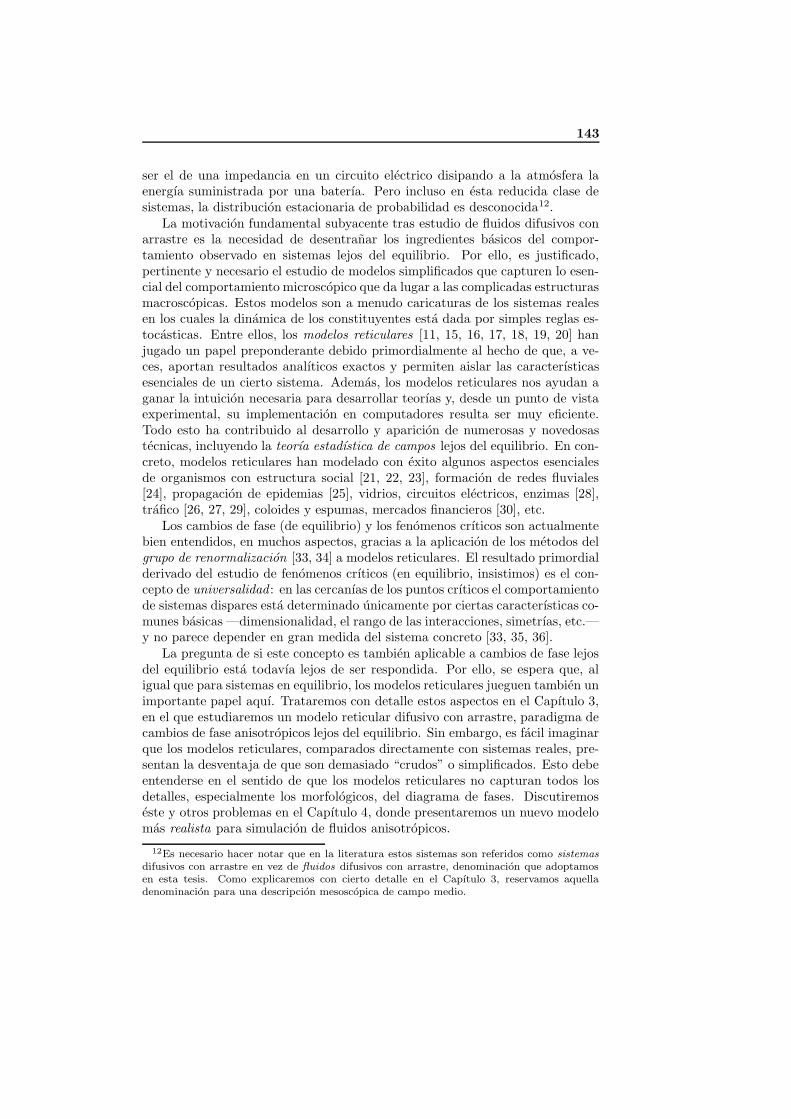
143
ser el de una impedancia en un circuito electrico disipando a la atmosfera laenergıa suministrada por una baterıa. Pero incluso en esta reducida clase desistemas, la distribucion estacionaria de probabilidad es desconocida12.
La motivacion fundamental subyacente tras estudio de fluidos difusivos conarrastre es la necesidad de desentranar los ingredientes basicos del compor-tamiento observado en sistemas lejos del equilibrio. Por ello, es justificado,pertinente y necesario el estudio de modelos simplificados que capturen lo esen-cial del comportamiento microscopico que da lugar a las complicadas estructurasmacroscopicas. Estos modelos son a menudo caricaturas de los sistemas realesen los cuales la dinamica de los constituyentes esta dada por simples reglas es-tocasticas. Entre ellos, los modelos reticulares [11, 15, 16, 17, 18, 19, 20] hanjugado un papel preponderante debido primordialmente al hecho de que, a ve-ces, aportan resultados analıticos exactos y permiten aislar las caracterısticasesenciales de un cierto sistema. Ademas, los modelos reticulares nos ayudan aganar la intuicion necesaria para desarrollar teorıas y, desde un punto de vistaexperimental, su implementacion en computadores resulta ser muy eficiente.Todo esto ha contribuido al desarrollo y aparicion de numerosas y novedosastecnicas, incluyendo la teorıa estadıstica de campos lejos del equilibrio. En con-creto, modelos reticulares han modelado con exito algunos aspectos esencialesde organismos con estructura social [21, 22, 23], formacion de redes fluviales[24], propagacion de epidemias [25], vidrios, circuitos electricos, enzimas [28],trafico [26, 27, 29], coloides y espumas, mercados financieros [30], etc.
Los cambios de fase (de equilibrio) y los fenomenos crıticos son actualmentebien entendidos, en muchos aspectos, gracias a la aplicacion de los metodos delgrupo de renormalizacion [33, 34] a modelos reticulares. El resultado primordialderivado del estudio de fenomenos crıticos (en equilibrio, insistimos) es el con-cepto de universalidad : en las cercanıas de los puntos crıticos el comportamientode sistemas dispares esta determinado unicamente por ciertas caracterısticas co-munes basicas —dimensionalidad, el rango de las interacciones, simetrıas, etc.—y no parece depender en gran medida del sistema concreto [33, 35, 36].
La pregunta de si este concepto es tambien aplicable a cambios de fase lejosdel equilibrio esta todavıa lejos de ser respondida. Por ello, se espera que, aligual que para sistemas en equilibrio, los modelos reticulares jueguen tambien unimportante papel aquı. Trataremos con detalle estos aspectos en el Capıtulo 3,en el que estudiaremos un modelo reticular difusivo con arrastre, paradigma decambios de fase anisotropicos lejos del equilibrio. Sin embargo, es facil imaginarque los modelos reticulares, comparados directamente con sistemas reales, pre-sentan la desventaja de que son demasiado “crudos” o simplificados. Esto debeentenderse en el sentido de que los modelos reticulares no capturan todos losdetalles, especialmente los morfologicos, del diagrama de fases. Discutiremoseste y otros problemas en el Capıtulo 4, donde presentaremos un nuevo modelomas realista para simulacion de fluidos anisotropicos.
12Es necesario hacer notar que en la literatura estos sistemas son referidos como sistemas
difusivos con arrastre en vez de fluidos difusivos con arrastre, denominacion que adoptamosen esta tesis. Como explicaremos con cierto detalle en el Capıtulo 3, reservamos aquelladenominacion para una descripcion mesoscopica de campo medio.

144 Resumen en Espanol
La segunda clase de sistemas considerados en esta tesis versa acerca de gasesgranulares agitados mecanicamente. Un medio granular [37] es un conglomeradode muchas partıculas de tamano macroscopico, y por lo tanto, susceptible de sermodelados clasicamente. Hay ejemplos por doquier y se presentan a muy difer-entes escalas: desde materiales polvoreados hasta nubes de polvo intergalactico.Dentro de ese intervalo podemos encontrar arena, hormigon, cereales, flujosvolcanicos, los anillos de Saturno y otros muchos ejemplos. Su importanciacientıfica y tecnologica es indudable, con numerosas aplicaciones farmaceuticas,en la construccion e ingenierıa civil, quımicas, agrarias y alimentarias, y, a mayorescala, en procesos geologicos y astrofısicos. Ademas, su estudio esta correla-cionado con otras clases de sistemas como coloides, espumas y vidrios. Ası puesla fenomenologıa mostrada por estos sistemas es amplısima, yendo desde unaspocas micras a miles de kilometros: formacion de patrones en granulados fluid-ificados [38, 39, 44], agregacion [42, 43], flujos y bloqueos en silos y tolvas [45],avalanchas y deslizamientos [46], mezcla y segregacion [47], conveccion [48, 49],erupciones [50, 51], por citar unos pocos. Por todo ello, su importancia estalejos de toda duda y la adecuada comprension de sus propiedades no es solo unanecesidad industrial urgente, sino que tambien supone un reto importante parala fısica.
Puesto que los granos individuales tienen dimensiones macroscopicas, lafriccion, deformacion, ruptura y las perdidas energeticas por colision producendisipacion de energıa, esto es, la energıa cinetica es transferida continuamente almedio en forma de calor. Asimismo, la escala de energıa tıpica para, por ejemplo,un grano de arroz de, digamos, longitud l ≈ 5mm y masa m es su energıa po-tencial mgl, donde g es la aceleracion gravitatoria. Es para tamanos de granomucho mas pequenos cuando otros tipos de interaccion ganan en importan-cia13. De ahı que en los medios granulares, y a diferencia de gases moleculares,la temperatura T no juega ningun papel, es decir, kBT mgl. Los efectosdinamicos pesan mas que cualquier tipo de consideraciones entropicas [37] y,consecuentemente, argumentos mecano-estadısticos o termodinamicos resultande poca utilidad. Ademas, dado que cualquier granulado esta formado por unnumero finito de constituyentes14, frecuentemente el efecto de las fluctuacionesen observables macroscopicos es enorme y, por tanto, su estadıstica es dominadapor los, ası llamados, eventos raros. Otros efectos tambien importantes estanrelacionados con el fluido intersticial, como aire o agua, aunque en muchas situa-ciones y, en buena aproximacion, puede ignorarse considerando unicamente lasinteracciones de grano con grano. En esta tesis (concretamente en la Parte II)nos restringiremos al estudio de sistemas granulares secos, donde la interaccionentre partıculas predomina sobre la interaccion con el posible fluido intersticial.
Sin embargo, y a pesar de la dinamica clasica que los caracteriza, los medios
13En granos con d ≈ 0.1 aparecen cargas electrostaticas superficiales, o para d ≈ 0.01 losefectos magneticos y de adhesion superficial comienzan a ser relevantes.
14A diferencia de gases moleculares, N NA donde N es el numero de partıculas y NA
el numero de Avogadro. No obstante, si N fuera lo suficientemente grande (a determinar ad
hoc) aun serıa posible emplear un tratamiento estadıstico.
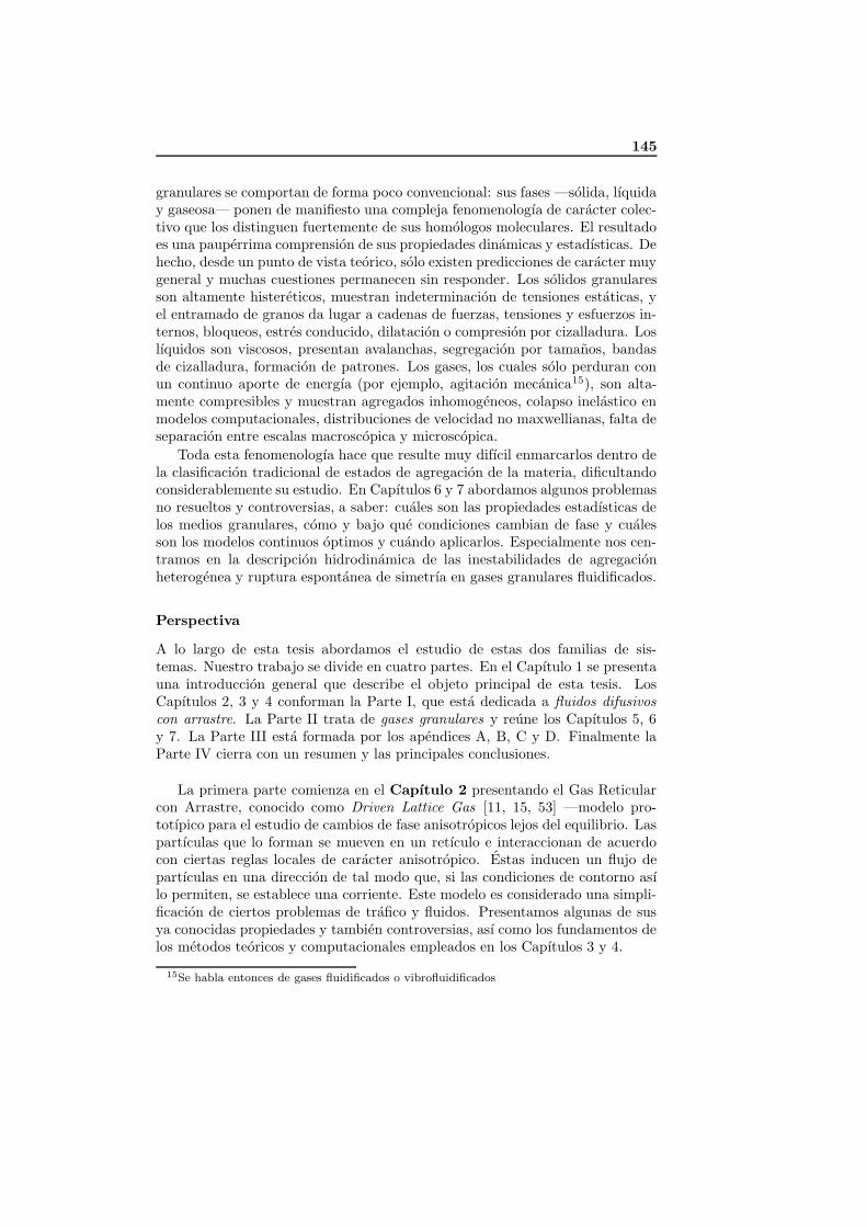
145
granulares se comportan de forma poco convencional: sus fases —solida, lıquiday gaseosa— ponen de manifiesto una compleja fenomenologıa de caracter colec-tivo que los distinguen fuertemente de sus homologos moleculares. El resultadoes una pauperrima comprension de sus propiedades dinamicas y estadısticas. Dehecho, desde un punto de vista teorico, solo existen predicciones de caracter muygeneral y muchas cuestiones permanecen sin responder. Los solidos granularesson altamente histereticos, muestran indeterminacion de tensiones estaticas, yel entramado de granos da lugar a cadenas de fuerzas, tensiones y esfuerzos in-ternos, bloqueos, estres conducido, dilatacion o compresion por cizalladura. Loslıquidos son viscosos, presentan avalanchas, segregacion por tamanos, bandasde cizalladura, formacion de patrones. Los gases, los cuales solo perduran conun continuo aporte de energıa (por ejemplo, agitacion mecanica15), son alta-mente compresibles y muestran agregados inhomogeneos, colapso inelastico enmodelos computacionales, distribuciones de velocidad no maxwellianas, falta deseparacion entre escalas macroscopica y microscopica.
Toda esta fenomenologıa hace que resulte muy difıcil enmarcarlos dentro dela clasificacion tradicional de estados de agregacion de la materia, dificultandoconsiderablemente su estudio. En Capıtulos 6 y 7 abordamos algunos problemasno resueltos y controversias, a saber: cuales son las propiedades estadısticas delos medios granulares, como y bajo que condiciones cambian de fase y cualesson los modelos continuos optimos y cuando aplicarlos. Especialmente nos cen-tramos en la descripcion hidrodinamica de las inestabilidades de agregacionheterogenea y ruptura espontanea de simetrıa en gases granulares fluidificados.
Perspectiva
A lo largo de esta tesis abordamos el estudio de estas dos familias de sis-temas. Nuestro trabajo se divide en cuatro partes. En el Capıtulo 1 se presentauna introduccion general que describe el objeto principal de esta tesis. LosCapıtulos 2, 3 y 4 conforman la Parte I, que esta dedicada a fluidos difusivoscon arrastre. La Parte II trata de gases granulares y reune los Capıtulos 5, 6y 7. La Parte III esta formada por los apendices A, B, C y D. Finalmente laParte IV cierra con un resumen y las principales conclusiones.
La primera parte comienza en el Capıtulo 2 presentando el Gas Reticularcon Arrastre, conocido como Driven Lattice Gas [11, 15, 53] —modelo pro-totıpico para el estudio de cambios de fase anisotropicos lejos del equilibrio. Laspartıculas que lo forman se mueven en un retıculo e interaccionan de acuerdocon ciertas reglas locales de caracter anisotropico. Estas inducen un flujo departıculas en una direccion de tal modo que, si las condiciones de contorno asılo permiten, se establece una corriente. Este modelo es considerado una simpli-ficacion de ciertos problemas de trafico y fluidos. Presentamos algunas de susya conocidas propiedades y tambien controversias, ası como los fundamentos delos metodos teoricos y computacionales empleados en los Capıtulos 3 y 4.
15Se habla entonces de gases fluidificados o vibrofluidificados

146 Resumen en Espanol
Una de las preguntas que cabe plantearse sobre cualquier modelo fısico es siel comportamiento que manifiesta es universal. En el Capıtulo 3 abordamosesta importante cuestion estudiando la segregacion anisotropica de fases en elmodelo prototıpico introducido en el Capıtulo 2. El enfasis de nuestro estudioesta puesto en la influencia de los detalles de la dinamica microscopica en elestado estacionario del no-equilibrio resultante, aunque tambien se presta ciertaatencion a aspectos cineticos. En especial trataremos, tanto desde un punto devista computacional como teorico, las similitudes y diferencias entre el drivenlattice gas y otros modelos reticulares y no reticulares relacionados con aquel.La comparativa nos permite discutir ciertas propiedades excepcionales y pocorealistas del modelo reticular original. Ademas, ponemos a prueba la validez dedos teorıas mesoscopicas actuales que pretenden dar cuenta del comportamientocrıtico de esta clase de sistemas.
En el Capıtulo 4 introducimos un novedoso modelo computacional defluido no reticular y de no-equilibrio disenado para el estudio de fenomenosanisotropicos. Su dinamica e interacciones son mas realistas que en, por ejem-plo, el driven lattice gas. Se trata de un modelo muy accesible desde el puntode vista computacional, que exhibe una corriente neta de partıculas y estruc-turas franjiformes a bajas temperaturas orientadas segun la direccion de uncampo externo, asemejandose a muchas situaciones reales. Describiremos tantolas propiedades cineticas a tiempos cortos (nucleacion) como las estacionariasdel modelo; en especial nos centraremos en su diagrama de fases: identificamosy caracterizamos sus fases solida (mono- y policristalina), lıquida y gaseosa, to-das ellas altamente anisotropicas. El calculo preciso de sus parametros crıticosnos lleva a discutir el papel de las simetrıas en el modelado de fluidos fuera delequilibrio con teorıas de campos y simulaciones. Ademas se esbozan algunascomparaciones con experimentos reales.
El Capıtulo 5 sirve de introduccion a la Parte II de esta memoria; parte quees dedicada a los gases granulares agitados mecanicamente o vibrofluidificados.Perfilamos el estado del arte con respecto a la investigacion en gases granulares.Concretamente discutiremos la aplicabilidad de las teorıas hidrodinamicas alestudio de flujos granulares. Tambien proporcionamos brevemente los ingredi-entes basicos de los modelos estudiados en los capıtulos siguientes y los metodosde simulacion.
En el Capıtulo 6 empleamos una descripcion hidrodinamica granular paraestudiar la fenomenologıa observada en un gas inelastico confinado en un recipi-ente anular sin gravedad. Nuestro principal proposito es caracterizar apropiada-mente sus estados estacionarios (de no-equilibrio) y establecer de forma precisaun diagrama de fases mediante la descripcion hidrodinamica y la computacional.Empleamos relaciones constitutivas de tipo Chapman-Enskog, derivadas estasde primeros principios. Prestamos especial atencion a las inestabilidades ob-servadas, a saber, separacion de fases, agregacion heterogenea de partıculas y
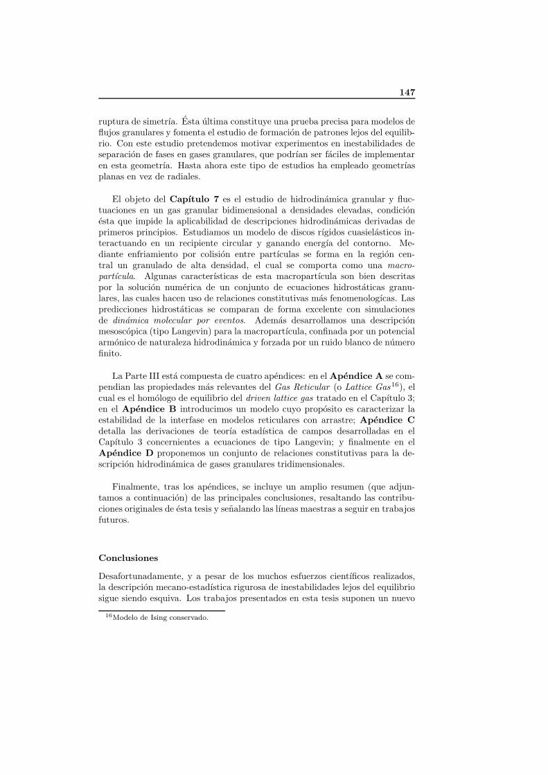
147
ruptura de simetrıa. Esta ultima constituye una prueba precisa para modelos deflujos granulares y fomenta el estudio de formacion de patrones lejos del equilib-rio. Con este estudio pretendemos motivar experimentos en inestabilidades deseparacion de fases en gases granulares, que podrıan ser faciles de implementaren esta geometrıa. Hasta ahora este tipo de estudios ha empleado geometrıasplanas en vez de radiales.
El objeto del Capıtulo 7 es el estudio de hidrodinamica granular y fluc-tuaciones en un gas granular bidimensional a densidades elevadas, condicionesta que impide la aplicabilidad de descripciones hidrodinamicas derivadas deprimeros principios. Estudiamos un modelo de discos rıgidos cuasielasticos in-teractuando en un recipiente circular y ganando energıa del contorno. Me-diante enfriamiento por colision entre partıculas se forma en la region cen-tral un granulado de alta densidad, el cual se comporta como una macro-partıcula. Algunas caracterısticas de esta macropartıcula son bien descritaspor la solucion numerica de un conjunto de ecuaciones hidrostaticas granu-lares, las cuales hacen uso de relaciones constitutivas mas fenomenologıcas. Laspredicciones hidrostaticas se comparan de forma excelente con simulacionesde dinamica molecular por eventos. Ademas desarrollamos una descripcionmesoscopica (tipo Langevin) para la macropartıcula, confinada por un potencialarmonico de naturaleza hidrodinamica y forzada por un ruido blanco de numerofinito.
La Parte III esta compuesta de cuatro apendices: en el Apendice A se com-pendian las propiedades mas relevantes del Gas Reticular (o Lattice Gas16), elcual es el homologo de equilibrio del driven lattice gas tratado en el Capıtulo 3;en el Apendice B introducimos un modelo cuyo proposito es caracterizar laestabilidad de la interfase en modelos reticulares con arrastre; Apendice C
detalla las derivaciones de teorıa estadıstica de campos desarrolladas en elCapıtulo 3 concernientes a ecuaciones de tipo Langevin; y finalmente en elApendice D proponemos un conjunto de relaciones constitutivas para la de-scripcion hidrodinamica de gases granulares tridimensionales.
Finalmente, tras los apendices, se incluye un amplio resumen (que adjun-tamos a continuacion) de las principales conclusiones, resaltando las contribu-ciones originales de esta tesis y senalando las lıneas maestras a seguir en trabajosfuturos.
Conclusiones
Desafortunadamente, y a pesar de los muchos esfuerzos cientıficos realizados,la descripcion mecano-estadıstica rigurosa de inestabilidades lejos del equilibriosigue siendo esquiva. Los trabajos presentados en esta tesis suponen un nuevo
16Modelo de Ising conservado.
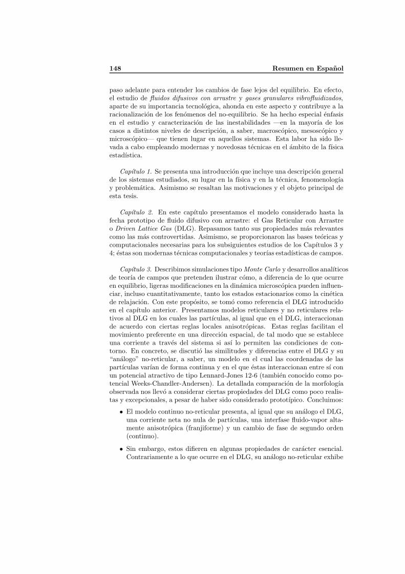
148 Resumen en Espanol
paso adelante para entender los cambios de fase lejos del equilibrio. En efecto,el estudio de fluidos difusivos con arrastre y gases granulares vibrofluidizados,aparte de su importancia tecnologica, ahonda en este aspecto y contribuye a laracionalizacion de los fenomenos del no-equilibrio. Se ha hecho especial enfasisen el estudio y caracterizacion de las inestabilidades —en la mayorıa de loscasos a distintos niveles de descripcion, a saber, macroscopico, mesoscopico ymicroscopico— que tienen lugar en aquellos sistemas. Esta labor ha sido lle-vada a cabo empleando modernas y novedosas tecnicas en el ambito de la fısicaestadıstica.
Capıtulo 1. Se presenta una introduccion que incluye una descripcion generalde los sistemas estudiados, su lugar en la fısica y en la tecnica, fenomenologıay problematica. Asimismo se resaltan las motivaciones y el objeto principal deesta tesis.
Capıtulo 2. En este capıtulo presentamos el modelo considerado hasta lafecha prototipo de fluido difusivo con arrastre: el Gas Reticular con Arrastreo Driven Lattice Gas (DLG). Repasamos tanto sus propiedades mas relevantescomo las mas controvertidas. Asimismo, se proporcionaron las bases teoricas ycomputacionales necesarias para los subsiguientes estudios de los Capıtulos 3 y4; estas son modernas tecnicas computacionales y teorıas estadısticas de campos.
Capıtulo 3. Describimos simulaciones tipo Monte Carlo y desarrollos analıticosde teorıa de campos que pretenden ilustrar como, a diferencia de lo que ocurreen equilibrio, ligeras modificaciones en la dinamica microscopica pueden influen-ciar, incluso cuantitativamente, tanto los estados estacionarios como la cineticade relajacion. Con este proposito, se tomo como referencia el DLG introducidoen el capıtulo anterior. Presentamos modelos reticulares y no reticulares rela-tivos al DLG en los cuales las partıculas, al igual que en el DLG, interaccionande acuerdo con ciertas reglas locales anisotropicas. Estas reglas facilitan elmovimiento preferente en una direccion espacial, de tal modo que se estableceuna corriente a traves del sistema si ası lo permiten las condiciones de con-torno. En concreto, se discutio las similitudes y diferencias entre el DLG y su“analogo” no-reticular, a saber, un modelo en el cual las coordenadas de laspartıculas varıan de forma continua y en el que estas interaccionan entre sı conun potencial atractivo de tipo Lennard-Jones 12-6 (tambien conocido como po-tencial Weeks-Chandler-Andersen). La detallada comparacion de la morfologıaobservada nos llevo a considerar ciertas propiedades del DLG como poco realis-tas y excepcionales, a pesar de haber sido considerado prototıpico. Concluimos:
• El modelo continuo no-reticular presenta, al igual que su analogo el DLG,una corriente neta no nula de partıculas, una interfase fluido-vapor alta-mente anisotropica (franjiforme) y un cambio de fase de segundo orden(continuo).
• Sin embargo, estos difieren en algunas propiedades de caracter esencial.Contrariamente a lo que ocurre en el DLG, su analogo no-reticular exhibe

149
una temperatura crıtica que decrece con la intensidad del campo externo.Es mas, a diferencia del DLG, no existe ningun cambio de fase en el lımitede campo externo saturante. En lo concerniente a los procesos cineticosde formacion de estructuras macroscopicas u ordenacion (nucleacion), seobservaron agregaciones de partıculas con forma triangular apuntando enel sentido del campo externo, justamente al contrario que en el modelodiscreto.
• Estas observaciones sugieren una falta de universalidad en el modelo retic-ular originario. Demostramos ası que el comportamiento del DLG estacondicionado en gran medida por la geometrıa del retıculo. Este es elagente que favorece la ordenacion, y no el campo en sı mismo. Por tanto, lacaracterıstica sorprendente y contraintuitiva de que en el DLG “el campoexterno” eleva la temperatura crıtica respecto a la del equilibrio no es sinoun efecto geometrico o topologico y no dinamico.
• De aquı se deriva, en concreto, que el DLG no tiene un homologo no-reticular (mas “realista”) inmediato.
• Para profundizar en esta situacion, se estudio el DLG bajo la accion deun campo externo saturante a la vez que se aumento el rango de las inter-acciones a nuevos vecinos. El modelo resultante, definido como NDLG17,se asemeja mas al del caso no-reticular: la temperatura crıtica decrececon el campo y las anisotropıas triangulares observadas en el proceso denucleacion a tiempos cortos se orientan en el sentido del campo.
• No obstante, mostramos que, aun ampliando el radio de interaccion entrepartıculas, tanto el decaimiento potencial de las correlaciones espacialescomo la criticalidad permanecen invariantes. Las primeras fueron moni-torizadas por la funcion de correlacion a dos cuerpos y por el factor deestructura, mientras que las propiedades crıticas se determinaron emple-ando tecnicas estandar de analisis de tamano finito y corroboradas por lateorıa mesoscopica de campos conocida como anisotropic driven system(ADS).
• Por consiguiente, al extender la dinamica en el DLG se modifica de formaesencial el diagrama de fases —el cual no puede ser determinado por crudosargumentos de simetrıas— pero no las propiedades intrınsecas relacionadascon la naturaleza de no-equilibrio del fenomeno —como el decaimiento delas correlaciones.
La conclusiones de este capıtulo estan complementadas apropiadamente por losresultados de criticalidad del modelo afın expuesto en el Capıtulo 4. Una posibley recomendable continuacion del trabajo desarrollado en este capıtulo es el estu-dio de la segregacion de fases en el modelo NDLG desde el punto de vista de lateorıa de campos empleando el enfoque de la teorıa ADS. Otros problemas son
17DLG con interaccion a vecinos siguientes o next-nearest-neighbors DLG.
150 Resumen en Espanol
el estudio detallado de la estabilidad de la interfase bajo campos intensos (veaseApendice B) y la extension de nuestros metodos a otros modelos reticularescomo, por ejemplo al Time Asymmetric Exclusion Process (TASEP) [16, 57].
Capıtulo 4. Puesto que, como fue demostrado en el capıtulo anterior, elDLG es poco realista en ciertos aspectos esenciales, presentamos aquı un modelonovedoso y mas realista de fluido con arrastre, ideal para el estudio de fenomenosanisotropicos. Se trata de un modelo no-reticular lejos del equilibrio en el quelas partıculas, que interactuan entre sı vıa un potencial tipo Lennard-Jones 12-6,son conducidas por la accion de un campo externo, cuya energıa se disipa en unbano termico. Estudiamos la cinetica de separacion de fases a tiempos cortosy sus diferentes fases estacionarias (altamente anisotropicas), a saber, solido(mono- y policristalino), lıquido y gas. En concreto, describimos los procesosde nucleacion, monitorizados por el exceso de energıa, el cual da cuenta de laenergıa interfacial; las propiedades estructurales de las diferentes fases en elestado estacionario, caracterizadas por las funciones de distribucion radial yazimutal y el grado de anisotropıa; y propiedades de transporte. Elaboramostambien una precisa estimacion de la curva de coexistencia lıquido–vapor y delos parametros crıticos asociados. Las principales conclusiones son:
• El modelo propuesto parece contener la fısica esencial y necesaria pararesultar util como un modelo prototıpico destinado a describir fenomenosanisotropicos observados en la naturaleza.
• Este modelo es mas conveniente para propositos simulacionales en flui-dos con arrastre que otros, como, por ejemplo, simulaciones estandar dedinamica molecular, que son mas costosas.
• El modelo es la extension natural a casos anisotropicos lejos del equilib-rio del conocido fluido de Lennard-Jones, que describe acertadamente elcomportamiento de gases reales como el Ar. En efecto, nuestro modelose reduce a este para campo cero. De otro modo, exhibe una corrienteneta de partıculas y estructuras macroscopicas franjeadas por debajo deun punto crıtico.
• En cuanto a las propiedades cineticas, y a pesar de la anisotropıa inher-ente del modelo en las etapas tardıas de la descomposicion espinodal, lanucleacion se produce por coagulacion tipo Smoluchowski y agregacion deOstwald, las cuales son conocidas por describir los procesos del nucleacionde fluidos reales en equilibrio.
• Inesperadamente, encontramos que el comportamiento crıtico del modeloes consistente con la clase de universalidad de Ising (equilibrio), pero nocon la del DLG. La principal razon de este aparente desacuerdo y de otrosdetallados en este capıtulo, podrıa ser la falta de simetrıa partıcula-huecoen el modelo Lennard-Jones con arrastre.
151
• De ahı inferimos que la discretizacion espacial puede cambiar de formasignificativa no solo las propiedades morfologicas y cineticas sino tambienlas propiedades crıticas. Esto contrasta fuertemente con el concepto deuniversalidad en sistemas en equilibrio, donde el comportamiento de estoscerca de los puntos crıticos es independiente de los detalles microscopicos.
• Finalmente, creemos que este modelo motivara nuevos experimentos de de-scomposicion espinodal anisotropica, ademas de nuevos trabajos teoricos.De hecho, nuestras observaciones, por ejemplo, en las propiedades es-tructurales y en las primeras etapas de la cinetica de segregacion defases, son facilmente accesibles por experimentos de espectroscopıa y mi-crocalorimetricos, respectivamente.
Muchas cuestiones quedan aun por desarrollar. Investigaciones adicionales, lascuales estan siendo elaboradas actualmente, involucran estudios detallados delas propiedades interfaciales y de los efectos de tamano finito. Otros problemasque serıa conveniente abordar en un futuro son dilucidar de forma precisa el pa-pel de la simetrıa hueco-partıcula y de la forma del potencial de interaccion enlas propiedades crıticas; analizar las etapas tardıas del proceso de segregacionde fases, ya estudiadas en otros sistemas en y fuera del equilibrio, [107, 108]y [103, 109], respectivamente; y estudiar, desde el punto de vista de la teorıade vidrios las caracterısticas morfologicas y estructurales de las fases solida yvidriatica (solido policristalino) que presenta nuestro modelo.
Capıtulo 5. En este capıtulo proporcionamos la base adecuada para nuestroestudio de gases granulares desarrollada en los Capıtulos 6 y 7. Discutimos algu-nas controversias, problemas abiertos y avances recientes en fluidos granulares,en particular, de la aplicabilidad de teorıas hidrodinamicas. Tambien presenta-mos los ingredientes basicos de los metodos computaciones implementados enlos siguientes capıtulos.
Capıtulo 6. Se presentaron calculos analıticos, ademas de simulaciones dedinamica molecular por eventos, para un granulado monodisperso confinado enun recipiente anular sin gravedad y forzado por una pared “termalizada”. Con-sideramos el lımite cuasielastico en una descripcion hidrodinamica que empleacoeficientes de transporte tipo Chapman-Enskog [135], derivables de primerosprincipios. Desarrollamos un estudio exhaustivo de las inestabilidades de agre-gacion heterogenea de partıculas, ruptura de simetrıa y separacion de fases queaparecen en el modelo, y que nos permiten determinar con exactitud su dia-grama de fases. Para comprobar y complementar las predicciones teoricas im-plementamos simulaciones de dinamica molecular por eventos para este sistema.Nuestro estudio nos lleva a desarrollar algunas consideraciones sobre la fısica delas inestabilidades que tienen lugar el modelo. De este capıtulo concluimos:
• El enfoque hidrostatico quedo completamente determinado por tres para-metros adimensionales: el de disipacion de energıa, la fraccion de areaocupada por los granos y la razon de aspecto del sistema.
152 Resumen en Espanol
• Nuestras simulaciones de dinamica molecular mostraron (mas claramentepara un numero suficientemente elevado de partıculas) la formacion deestados agregados con simetrıa azimutal alejados de la pared termicaque fuerza al granulado. A pesar del (relativamente) escueto numero departıculas empleado, estos estados anulares fueron descritos de forma pre-cisa y para densidades moderadas por la solucion numerica de las ecua-ciones hidrostaticas propuestas, las cuales emplean relaciones constitutivastipo Enskog.
• Mediante un analisis de estabilidad marginal se obtuvieron solucionesque bifurcan del estado mas basico (el estado anular). Dicho de otromodo, estas soluciones predicen la ruptura espontanea de simetrıa deaquellos estados con simetrıa azimutal (inestables respecto de pequenasperturbaciones), hecho que ocurre solamente en un determinado rangode parametros. Determinamos las curvas de estabilidad marginal y lascomparamos con las fronteras de la region espinodal (de compresibilidadnegativa) del sistema.
• Se concluye que el mecanismo fısico de la inestabilidad de separacion defases es la compresibilidad negativa del granulado en la direccion azimutal,causada por las perdidas de energıa en las colisiones. Matematicamente, laseparacion de fases se manifiesta en la existencia de soluciones adicionalesen cierta region del espacio de parametros a la ecuacion de densidad.
• Tambien las simulaciones mostraron la existencia de separacion de fases,predichas por la descripcion hidrodinamica, pero enmascaradas por grandesfluctuaciones espacio-temporales. Midiendo la distribucion de probabili-dad para la amplitud del modo de fundamental del desarrollo de Fourierdel espectro azimutal de la densidad de partıculas, identificamos con clar-idad el cambio de estados simetricos a estados con separacion de fases.
• Ademas encontramos que la region del espacio de parametros asociada a lainestabilidad, predicha por la descripcion hidrodinamica, se localiza dentrode la region de separacion de fases observada en nuestras simulaciones.Esto implica la presencia de una region binodal (de coexistencia de fases)donde el estado anular es metaestable.
• Esperamos que las inestabilidades de agregacion, ruptura de simetrıa yseparacion de fases sean facilmente observables en experimentos. De he-cho, el modelo aquı propuesto es experimentalmente accesible, de modoque podrıa motivar nuevos experimentos en estas inestabilidades si atra-jese la atencion de la comunidad pertinente.
Es claro que la comparacion de las predicciones de nuestra teorıa y simulacionescon experimentos serıa altamente interesante. Al proponer la geometrıa anularesperamos motivar estudios experimentales de estas inestabilidades que podrıanresultar ventajosos en esta geometrıa. Un dispositivo experimental anular no
153
presenta paredes laterales (como en una geometrıa rectangular) y por tanto evi-tarıa las innecesarias, e inevitables por otro lado, perdidas por colision con laspartıculas. Un posible experimento podrıa emplear esferas metalicas deslizandosobre una superficie cuasi-plana (ligeramente concava). La pared termica podrıaser implementada por una anillo ligeramente excentico (y quizas rugoso) rotandorapidamente. Igualmente interesante para estudios subsiguientes serıa determi-nar la naturaleza de las soluciones que se bifurcan (¿sub- o supercrıticamente?)del estado agregado con simetrıa azimutal. Otros estudios podrıan explotar lassimilitudes entre la fenomenologıa observada en nuestro modelo y la de los anil-los planetarios, en los cuales, tambien se observan inestabilidades de agregaciony de ruptura de simetrıa, entre otras.
Capıtulo 7. En este capıtulo tratamos con hidrodinamica granular y fluctua-ciones en un sencillo gas granular bidimensional donde, debido a densidades ele-vadas (y no a inelasticidad elevada), descripciones continuas basadas en primerosprincipios dejan de tener validez. Los enfoques hidrodinamicos fueron puestosa prueba en un caso extremo empleando simulaciones de dinamica molecularpor eventos: cuando se forman agregados granulares cuya densidad es proximaal valor de empaquetamiento maximo (denominados macropartıculas). El sis-tema modelo considerado esta formado por discos rıgidos inelasticos encerradosen un recipiente circular cuya pared esta termalizada forzando al granulado yllevandolo lejos del equilibrio. Las principales conclusiones se resumen en:
• Simulaciones de dinamica molecular mostraron, a causa del enfriamientopor colisiones, un agregado fuertemente empaquetado de partıculas, conuna interfase cuasicircular abrupta, con fluctuaciones espaciales y ais-lado de la pared termica por un gas muy diluido. La formacion de lamacropartıcula requiere un cierto numero de partıculas y la transicion, enfuncion de la densidad, desde un estado (cuasi) homogeneo a la macropartı-cula es abrupta pero continua.
• Se resolvio numericamente un conjunto de ecuaciones granulares hidrostati-cas que emplean como relaciones constitutivas las fenomenologicas deGrossman et al. [154]. Encontramos que, en un amplio rango de parametros,el ajuste —incluyendo la parte de maximo empaquetamiento— con lasolucion con simetrıa azimutal de las ecuaciones hidrostaticas es casi per-fecto. Tambien demostramos que, para el mismo sistema, el empleo derelaciones constitutivas tipo Enskog [135], derivables de primeros princip-ios, no describe adecuadamente —mediante comparacion directa con losresultados de simulacion— la region de mayor densidad del granulado.
• Estos resultados, que estan de acuerdo con resultados previos en ge-ometrıas planas con y sin gravedad, extienden la aplicabilidad de lasrelaciones constitutivas de Grossman et al. a coeficientes de restitucionligeramente menores y a geometrıas no planas.
• Un analisis de estabilidad marginal demostro —independientemente de lasrelaciones constitutivas empleadas— que no hay soluciones estacionarias
154 Resumen en Espanol
que bifurquen linealmente de la de simetrıa azimutal, esto es, no hayestados que manifiesten ruptura de simetrıa alguna. Esto esta de acuerdocon la persistencia de macropartıculas circulares y cuasicirculares que seobservan en nuestras simulaciones.
• Estudiamos, por primera vez, las fluctuaciones de las macropartıculas,midiendo la distribucion de probabilidad radial del centro de masas delsistema. Las fluctuaciones resultan ser gaussianas.
• Las fluctuaciones gaussianas observadas del centro de masas sugieren unadescripcion mesoscopica tipo Langevin en terminos de una macropartıculaconfinada un potencial atractivo de naturaleza hidrodinamica y forzadapor ruido de numero finito —queremos decir que el agregado efectua unmovimiento browniano dentro del sistema. Se determino la correspondi-ente ecuacion de Langevin.
• En contra de lo que ocurre en sistemas en equilibrio —y en muchos lejosdel equilibrio—, en los cuales la magnitud relativa de las fluctuacionesdecrece al incrementar el numero de partıculas18, encontramos que lasfluctuaciones persisten al incrementar el numero de partıculas.
Aun quedan algunos problemas en nuestro modelo circular. Una cuestion quedeberıa ser tratada es si existen inestabilidades adicionales en este sistema mod-elo. Algo de intuicion podrıa obtenerse, por ejemplo, mediante medidas de or-den posicional y orientacional del agregado, siguiendo la analogıa con la teorıaKTHNY [119] para fusion o licuefaccion en sistemas en equilibrio. Concreta-mente, estas podrıan llevarse a cabo monitorizando las respectivas funciones decorrelacion. Es posible que tanto una solucion general dependiente del tiempocomo un estudio de estabilidad no-lineal contribuyan a la busqueda. Otrosposibles trabajos futuros son el estudio de inestabilidades en modelos tridimen-sionales relacionados (en el Apendice D se incluye una primera aproximacion aeste tema) y de la fenomenologıa mostrada por gases granulares polidispersosen este tipo de sistemas.
A pesar de que comunmente los apendices se relegan a un segundo plano,creemos que nuestros Apendices B y D merecen sus propias conclusiones.
Apendice B. Recordamos que en este apendice presentamos un modelo difu-sivo y con arrastre cuyo proposito es comprender mejor el balance entre campoexterno y bano termico que ocurre en el DLG y en otros modelos relaciona-dos (concretamente, los modelos reticulares estudiados en el Capıtulo 3). Losprincipales resultados son:
• Estudiamos la estabilidad de la interfase (orientada segun la direccion delcampo) en el lımite de campos saturantes, encontrando un cambio de fase
18Para un gas ideal en equilibrio: σ ∼ O(N−1/2), donde σ es la magnitud relativa de lasfluctuaciones y N es el numero de partıculas.
155
de segundo orden geometrico o topologico en funcion de la conectividad delos sitios del retıculo. Para bajas conectividades existe orden, dominan losefectos termicos y la interfase es estable, mientras que al incrementar laconectividad (por encima de un valor crıtico) el orden desaparece, dominael campo externo y la interfase se vuelve inestable.
• Este cambio de fase geometrico confirma que el balance campo–temperaturano es tan sencillo como la dinamica microscopica sugiere, es decir, no esuna mera superposicion lineal de ambos. Este hecho es una manifestacionclara de una dinamica colectiva emergente.
• Ademas se determinaron los parametros crıticos del cambio de fase.
Apendice D. En este apendice desarrollamos una serie de estudios teoricospara mostrar la existencia de inestabilidades de agregacion y ruptura de simetrıaen flujos granulares tridimensionales. De hecho, se trata de una sencilla ex-tension a tres dimensiones de la geometrıa circular estudiada en el Capıtulo 7.Ası, el modelo es el de un gas de esferas rıgidas colisionando inelasticamente enel interior de un cilindro cuya pared curva esta termalizada. Para este estudio,se hizo necesario proponer un nuevo conjunto de relaciones constitutivas.
• Derivamos relaciones constitutivas para gases granulares tridimensionalesempleando argumentos de volumen libre en la vecindad de la densidad demaximo empaquetamiento, y sugerimos una interpolacion entre el lımitede maxima densidad y las relaciones usuales en el lımite diluıdo. Para ellonos basamos en la estrategia seguida por Grossman et al. [154] en dosdimensiones, que emplea tecnicas de volumen excluıdo para determinarlas relaciones constitutivas.
• Mediante los metodos desarrollados en los Capıtulos 6 y 7 pronosticamosy caracterizamos las inestabilidades de agregacion y ruptura de simetrıaen un recipiente cilındrico. La presencia de esta ultima supone una grandiferencia con lo observado en el Capıtulo 7, donde su homologo bidimen-sional no presentaba ruptura de simetrıa alguna.
Publicaciones
Los estudios descritos en esta tesis han dado lugar a las siguientes publicaciones:
• Manuel Dıez-Minguito, Pedro L. Garrido, and Joaquın Marro, Lennard-Jones and lattice models of driven fluids, Phys. Rev. E 72, 026103 (2005).
• Joaquın Marro, Pedro L. Garrido, and Manuel Dıez-Minguito, Nonequili-brium anisotropic phases, nucleation and critical behavior in a drivenLennard-Jones fluid, Phys. Rev. B 73, 184115 (2006).
• Manuel Dıez-Minguito, Pedro L. Garrido, and Joaquın Marro, Lattice ver-sus Lennard-Jones models with a net particle flow in Traffic and GranularFlows ’05, in press (Springer, Berlin, 2006).

156 Resumen en Espanol
• Baruch Meerson, Manuel Dıez-Minguito, Thomas Schwager, and ThorstenPoschel, Close-packed granular clusters: hydrostatics and persistent Gaus-sian fluctuations, submitted to Europhys. Lett. (2006)
• Manuel Dıez-Minguito and Baruch Meerson, Phase separation of a drivengranular gas in annular geometry, submitted to Phys. Rev. E (2006).
• Manuel Dıez-Minguito, Pedro L. Garrido, Joaquın Marro, and Franciscode los Santos, Driven two-dimensional Lennard-Jones fluid in ModelingCooperative Behavior in the Social Sciences, P. L. Garrido, J. Marro, M.A. Munoz (eds.), AIP Conference Proceedings 779, 199 (2005).
• Manuel Dıez-Minguito, Pedro L. Garrido, Joaquın Marro, and Franciscode los Santos, Simple computational Lennard-Jones fluid driven out-of-equilibrium, in XIII Congreso de Fısica Estadıstica’ FISES’05, AbstractBook (2005).
• Manuel Dıez-Minguito, J. Marro, and P. L. Garrido, On the similari-ties and differences between lattice and off-lattice models of driven fluidsin Workshop on Complex Systems: New Trends and Expectations, to bepublished in Euro. Phys. J.-Special Topics (2006).
• Manuel Dıez-Minguito and Baruch Meerson, Phase separation of a drivengranular gas in annular geometry, in XIV Congreso de Fısica EstadısticaFISES’06, Abstract Book (2006).
Los siguientes trabajos se encuentran en preparacion:
• Manuel Dıez-Minguito, A. Achahbar, Pedro L. Garrido, and Joaquın Marro,Langevin-type description for the driven lattice gas with next-nearest-neighbordynamics (2006).
• Manuel Dıez-Minguito and Thorsten Poeschel, On the validity of globalequations of state for driven granular gases (2006).
• Manuel Dıez-Minguito, Pedro L. Garrido, and Joaquın Marro, Interfacialproperties in a nonequilibrium microfluidic system (2006).
Este trabajo ha sido financiado parcialmente por el Ministerio de Educacion yCiencia (MEC) de Espana y fondos FEDER (proyecto FIS2005-00791).