BIT 25 (1985). 113-134 1 4

I) i I

APPROXIMATE COUNTING: A DETAILED ANALYSIS ,

PHILIPPE FLAJOLET INRIA, Domaine de Voluceau-Rocquencourt, B.P. 105, 78153 Le Chesnay CEDEX, France

Abstract. Approximate counting is an algorithm proposed by R. Morris which makes it possible to

keep approximate counts of large numbers in small counters. The algorithm is useful for gathering statistics of a large number of events as well as for applications related to data compression (Todd et al.). We provide here a complete analysis of approximate counting which establishes good convergence properties of the algorithm and allows to quantify precisely complexity-accuracy tradeoffs.

Introduction.

As shown by an easy information-theoretic argument, maintaining a counter whose values may range in the interval 1 to M essentially necessitates log,M bits. This lower bound is of course achieved by a 1 standard binary counter. R. Morris [8] has proposed a probabilistic algorithm that maintains an approximate count using only about log,log,M bits. This paper is devoted to a detailed analysis of characteristic parameters of that algorithm. We provide precise estimates on the probabilities of errors, from which the soundness of the method can be assessed _and complexity-accuracy trade-offs can be quantified.

The algorithm itself is useful for gathering statistics on a large number of events in a storage efficient way [SI. It was proposed for applications to data compression [9] when building an adaptive encoding scheme to represent ~~~~~- random” data (see e.g. [4] for adaptive Huffman codes and [7] for arithmetic coding); there, typically a large number of counters need to be maintained to gather statistics on the data to be compressed, but high accuracy of each counter is not a critical factor in the design of almost-optimal codes. Actually Todd et al. report the overall performance of a system using approximate counting which is only 4 few percent off a reference system using exact counts.

There are other cases like data base systems where probabilistic counting methods prove useful. We mention a related algorithm; called ‘‘Probabilistic Counting” that has been proposed in [3]. This algorithm makes it possible to determine the approximate value of the number of distinct elements in a file in a single pass using a few operations per element and only O(1) additional storage.

Received October 1982. Revised August 1984.

114 PHILIPPE FLAJOLET

The plan of the paper is as follows. We start with a simple version of the algorithm: approximate counting with base 2, which is very easy to implement on a binary computer. It appears (Theorems 1, 2) that this algorithm can maintain an approximate count up to M using about log,log,M bits, with an error that is typically of one binary order of magnitude.

The analytic techniques that we use in Sections 2, 3, 4, involve manipulation of generating functions related to a discrete time birth-txocess to which the algorithm is equivalent, certain properties of the Mellin integral transform, and finally some simple identities that properly belong to the theory of integer partitions. In Sections 5, 6,.we discuss the more general version of the algorithm with an arbitrary base. The analysis shows that, using suitable corrections, one can count up to M keeping only log, log,M + 6 bits with an accuracy. of order O(2 -

A preliminary report on this work has been presented at the International Seminar on Modelling and Performance Evaluation Methodology (“On Approximate Counting” : Proceedings, Volume 2, pp. 205-236, Paris, January 1983).

+

1. Approximate counting with a binary base. -

If the requirement of accuracy is dropped, a counter of value n can be replaced by another counter C containing hog,nJ which only requires storing about log, log, n bits. However since the fractional part of log, n is no longer preserved, there now arises the problem of deciding when to update the logarithmic counter in the course of successive incrementations. The idea of [8], [9] is to base this decision on probabilistic choices.

Approximate counting starts with counter C initialized to 1. After n increments, we expect C to contain a good approximation to hog, nJ ; we should thus increase C by 1 after another n increments approximately. Since the exact value of n has not been kept and only C is known, the algorithm has to base its decision on the content of C alone. Approximate counting then treats the incrementation by the following procedure.

L. -

procedure increment (C : integer) ;

Let DELTA (C) be ajandorn variable w hkh takes value 1 with probability 2-‘ and value 0 wrth probabi */ i tv 1 -2-‘; C := C+DELTA (C)

The interesting fact about this procedure is the following: if C, is the random variable representing the content of counter C after n applications of the increment procedure, then the expectation of 2 c n bears a simple relation to n (as we shall prove at the end of Section 2).

I

APPROXIMATE COUNTING : A DETAILED ANALYSIS 115

PROPOSITION 0 [SI : The expectation and variance of 2cn satisfy

‘% E(2Cm) = n + 2 ; a2(2Cn) = n(n+ 1)/2. - ..

Thus 2‘-2 represents an gnbiased estimator of n. In the sequel, we give a detailed analysis of the probability distribution of C, and characterize its mean and variance.

THEOREM 1. has average value

After n successive increments, the counter of approximate counting

1, C, = log, n + y / M - R + + + 0(10g2 n ) + O(n -0 .98

where ;1 = En I 1/(2” - 1) = 1.6067, ..., y = 0.577721,. . ., is the Euler constant, and w is a periodic function of mean value 0 and amplitude less than 10- ’.

The constant after log2n gives the asymptotic drft of C, compared to log,n, and its numerical value is - 0.27395, . . . ; furthermore, calculations developed hereafter show that the actual drift for finite n varies very little with n : for n = 10, 100, 20000, the values of cn-log2n are respectively +0.0453,

Another interesting feature of the algorithm is the relatively low dispersion of - 0.2383, -0.2737. *

i the results it produces. We can prove:

THEOREM 2. After n successive increments, the standard deviation of the contents of the counter satisfies

0; = 0: +n(10g2 n ) +o(I),

where 0, = 0.8736, ... is a constant and n is a periodic function of mean value 0 and amplitude less than The constant 0, has the explicit expression

I l c

1 +- - - - (2”-1)2 12 1 0 g 2 ~ , , ksinh(8k)’

n2 2” 2 - 0, -

6 b 2 2 n z 1 -

In particular,’ corresponding to n = 10, 100, 2oo00, we have 0, = 0.7776, 0.8618, 0.8734. Thus typically C , estimates log,n with an error less than 1.

Finally, the methods developed here also permit evaluation of the probabilities of error. The distribution of values of approximate counting after n increments appears to be fairly narrowly centered around the average (better than merely predicted from the variance analysis using the Chebyshev inequalities), and for

I16 PHILIPPE FLAJOLET

instance in the case of n = 1024 (so that log,n = 10) the following probabilities for the counter values, determined by Proposition 1 below, are:

. ,

counter value 7 8 9 10 11 12 13

probability 0.001 1 0.0602 0.3424 0.4218 0.1538 0.0195 O.OOO1

Thus in that case C, will differ from log,n by more than 1 unit in only 8 % of the cases. More generally, Proposition 3 provides a sort of limiting distribution result for the probabilities of counter values. r'

2. Basic probabilities.

The possible evolutions of the algorithm can be seen as an evergrowing tree: we start from the counter set to 1 ; from this two situations cag result: either the counter keeps its value 1 (this has probability i) or it is increased to 2 (with probability i); each of these possible stages has itself two possible outcomes. The corresponding tree of possibilities'is given in Figure 1, with edges labelled with the probabilities of corresponding transitions. From it, we see for instance that when n = 3, the probabilities of observing counter values 1, 2, 3, 4 are respectively 64, 64, 64, 64.

8 3 8 1 7 1

d

/ /

Fig. 1. The possible evolutions of approximate counting for n = 1,2,3.

APPROXIMATE COUNTING : A DETAILED ANALYSIS 117

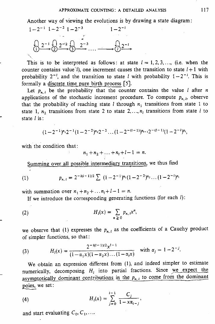
Another way of viewing the evolutions is by drawing a state diagram : 1 - 2 4 1 - 2 4 1 - 2 3 1 -2-1

.. n 2 - 1 n 2-' 2-3 n 2-1 @-@i@- .... ---..(&.-+ \ '.

This is to be interpreted as follows: at state 1 = 1,2,3, . . ., (i.e. when the counter contains value''I), one increment causes the transition to state 1 + 1 with probability 2-', and the transition to state I with probability 1 -2-'. This is formally a discrete time pure birth process [SI.

Let pn,I be the probability that the counter contains the value 1 after n applications of the stochastic increment procedure. To compute pn, ,, observe that the probability of reaching state 1 through n, transitions from state 1 to state 1, n2 transitions from state 2 to state 2, ..., n, transitions from state 1 to state 1 is:

with the condition that: n,+n,+ ...+ n , + l - l = n.

Summing over all possible intermediary transitions, we thus find

(1) P n . 1 - - 2-1(1-1)/2 (1-2-')"1(1-2-2)"2 ...( 1-2-94

with summation over n, + n2 + . . . n, + 1 - 1 = n. If we introduce the corresponding generating functions (for each l ) :

we observe that (1) expresses the pn , I as the coefficients of a Cauchy product of simpler functions, so that:

~ - 1 ( 1 - 1 ) / 2 - , - 1 L . - . A with aj = 1 -2-j.

( l - o ! l x ) ( l - a 2 x ) . . . ( l - a I x ) Hl(4 =

We obtain an expression different from (l), and indeed simpler to estimate numerically, decomposing H , into partial fractions. Since we exEect the ,asymptotically dominant contfibutions in the pn, , to come from the dominant e w e set:

(4)

and start evaluating Co, C1,. . ..

118 PHILIPPE FLAJOLET

We have

Cj = lim, -, a;;jHl(x)( 1 - a l - , ~ ) , SO that

co = 2-W-1)P (1 - 2 - yl- l ) ( 1 - al/al) - (1 - a,/Cc,)- l . . . (1 - a* - &*)- 1

which after simplification using (a1 - a j ) = 2-j( 1 - 2 - 9 gives : * 1 -1 Co = (1 -r) (1 - 1 /4)- . . . ( 1 - 2-(' - " ) - '.

Similarly, we find in general

- (- 1 ) Q - j ( j - 1 ) / 2 ~ , : 1 ~ - 1 (5) cj - l - l - j ,

where for all k : k

Q k = n ( 1 - 2 - i ) , and Qo = 1. i = l '

Now from (4), there immediately follows an expression for the coefficients p n , l of H l ( x ) :

I - 1

I

whence with (5 ) , (6):

PROPOSITION 1. The probability p n , I of having counter value 1 after n increments is I - 1 i 1 - 1 - j

This expression permits an easy numerical calculation of the probabilities involved -. - in approximate counting. We notice also that from their definition the quantities pn , satisfy the recurrence :

P n + 1 . I - - (1 -2 -1 )pn ,1+2- (1 -1 )p" ,1 - 1

from which by induction follows the already mentioned equality :

E(2C.) = n + 2 .

3. Continuing with approximations.

The expression of Proposition 1 is not as bad as it looks. First the product

(8) 03 ~

Q = n (1-2-i) i = 1

APPROXIMATE COUNTING : A DETAILED ANALYSIS I19

is convergent and simple comparisons with the geometric series show that

IQ-Qkl = o(2-")

with Qk defined in (6). In particular the Qk are always in the interval defined by Q = 0.288788, ... and 1, and the denominators in (7) are bounded.

Second, the very fast decrease of the coefficients 2-j(j-')I2 shows that numerically the significant contribution comes from small values of the index j, and asymptotically only values of j less than O(Jlog,n) need to be considered.

Last, the exponential approximation (1 -a)n !E e -an is usually justified in this class of problems (see e.g. [6, p. 1311).

We first prove that for I small enough compared to n, the probabilities pn, [ are small.

\

- ..

PROPOSITION 2. For 1 < log, n - 2 log, In n, the probabilities pn. I satisfy p, , I = O(ln n exp( - (In n)'))

uniformly in n and 1.

PROOF. Since we have (1-2-')" > (1-2/2')" > (1-4/2')" > ... and Qk > Q for all k , the pn, i can be bounded by

(9 1 . p,,! < Q-21(1 -2-9" = Q-'lexp(nln(1-2-')).

Now observing that for

we obtain from (9): ~ € 1 0 ; I[ :exp(nln(l - u ) ) = exp(-nu-nu2/2- ...) < e-"",

pn,I < Q-21exp(-n2-i) = O(lnnexp((-lnn)'))

which is thus exponentially small. Now when I is large enough, we can prove that the pn, l approach a

limiting distribution in the following sense :

PROPOSITION 3. Let be the function defined by

Then for 1 > log, n - 2 log, In n, we have pn, = +(nZ-')+ O(n-0*99) where the O(. ) term is unform in n and 1.

120 PHILIPPE FLAJOLET

PROOF. The proof proceeds by stages using the previously mentioned approxi- f ' y

mations. .

(i) Truncation of the sum: let r = r (n) = 2(10g2 n)ll2. We set 3

- r

PA,, = c ( - 1 Y 2 - j ( j - 1 112 Q,: 1 ~ - $ - j ( 1 - 2 - ( l -~ ' )y j = 0

(10)

Obviously

(ii) Simplification of the denominators : define

using the fact that IQ-Ql - l - j l = 0 ( 2 - ' + ' + j ) since the sum of ( r + 1) terms:

comprises

(iii) Using the exponential approximation: given the conditions on I and j , u = 2-('-'' is always small, so that:

'

1

since nu2 < 1 for n large enough. Thus setting:

(14)

we have

(iv) Complzting the sum: majorization of (1 l), we find :

is a partial sum of 4 ( n 2 - ' ) ; using again the

(16) Ip;,',-4(n2+)1 = o(n-2).

Thus putting together equations (10) to (16) proves Proposition 3.

Finally we need information on the tail of the distribution, corresponding to values of I larger than log,n.

APPROXIMATE COUNTING A DETAILED ANALYSIS 121

PROPOSITION 4. uniformly in n and 6.

For l = 210g2n+6 with 6 2 0, we have pn,' = O(2-%-Oeg9 1

PROOF (sketch). ~ The prodf mimics the previous one; let us choose this time

r = log,n+6 \

as the splitting value for the index in the sum giving p n , l . In part (i), we now have :

I I - 1 I

Parts (ii) and (iii) now lead to error bounds of the form O ( 2 - d n - 0 * g g ) since

Finally we can again complete the sum as in (iv) introducing error terms of

We have thus proved:

2-('-J> = O(n- ' ) .

the form (17).

(18) ; pn, = $ ( n 2 - i ) + O ( 2 - d n - 0 . 9 9 ) .

Since $ ( x ) is clearly differentiable at x = 0, y e have

Thus combining (18 ) and (19 ) completes the proof of the proposition. 4 In the sequel we shall Geed properties of the function $. Some of them appear

to be related to classical identities in the theory of partitions. Our starting point is the following identity [ 13 :

(with the usual convention for k = 0 that an empty product is equal to 1). Equation (20 ) is also valid analytically for all u, provided that It1 The coefficient of uktn in the left hand side member counts the number

of partitions of the integer n into distinct parts and, with a simple transformation on partitions, the right-hand side can be similarly interpreted (see also [ l ] for an algebraic proof'). Instantiating (20 ) with u = - 1 and t = 1/2, shows that

1 .

and thus +(O) = 0 as could be expected. We shall also need the following

122 PHILIPPE FLAJOLET

identities :

= - (1 -$)( 1 -a)( 1 -+) . . .,

a3 1

= 2[(1 --$)(I -a)(l-+). . .] 1 -2- n = l 2"-1'

which are easily obtained by successive differentiation of (20) with respect to u, 1 setting then u = - 1 and t = 7. -- .

4. Determination of asymptotic exGansions.

function F is defined for all x 2 0 by: The developments above suggest approximating cn with the value F ( n ) where

F ( x ) = l@(x2-l). J

121 (24)

For large x, F can be estimated using Mellin transform techniques. We first prove

LEMMA 1. The expected value cn satisfies: cn = F(n)+O(n-0*98) .

PROOF. Let us define the 3 intervals:

I , = [l,1og2n-21og,lnn[

I , = [log, n - 2 log, In n, 2 log, n[

1, = [2log,n, [ 9

and for j = 1,2,3:

c'j' = c ip", 1 : P' = l 4 ( 2 3 I ) . le I , l e i ,

By Proposition 2, we have:

APPROXIMATE COUNTING A DETAILED ANALYSIS 123

and by Proposition 4: - \ \

The three last equalities imply Lemma 1. a We are thus left with estimating the behaviour of F(x),as given by (24). To that

purpose, we use the Meffin integral transform which for a real function f is defined by (see [2]):

- (25) f * ( s ) = J l [ f ( x ) ; s] = l; f ( x ) X ” - ‘dx .

This transform is useful for studying harmonic sums like (24) : from the obvious functional property

(26) Jl[f(ax);s] = a--”f*(s), a > 0,

J

it follows formally that the Mellin transform of F is

F*(s) = ( I2’”4*(s). 1 2 1

The Mellin transform of 4 is itself computed using (26) repeatedly: from the definition of 4 (again formally) we expect

since, as is classicaIly known [lo] : J

k4) Thus formally, we have: -

(30) F*(s) = 2T(S)(2“- l ) - 2 t ( S ) ,

where

124 C. PHILIPPE FLAJOLET

Analytical1y:the . r integral in (29) is defined for Re(s) > 0. For s: - 1 < Re(s) < 0, we have -

- (e-x- l)xs-'dx = f(s). Using (21), we also have

8

.\

; ! - a , 4(x) = Q-' (-1Y'2-j(j-1)/2Q,~1iexp(-2j~-1), j 2 0

whence the integral defining the Mellin transform of d is defined for - 1 < Re(s) < 0. Actually (28) holds for any s,Re(s) > - 1, and 4* has a removeable singularity at s = 0. It is finally easy to see that (27) hdds provided the sum there is convergent, which requires Re(s) < 0. Thus equations (30), (31) are justified for s in the strip - 1 < Re@) < 0; there the integral of the f9rm (25) expressing F*(s) is absolutely convergent.

The singularities of F*(s) are related to the terms in the asymptotic expansion of F ( x ) when x -, co [2]. To see that, we use the inversion theorem for Mellin transforms which gives

F(x) = - F* (s)x - SdS, (32) ~ 2rn r+im d - i c o

where d can be taken arbitrarily inside the domain of absolute convergence of the integral giving F*(s). Here, we may take any d in the interval ] - 1, O[.

By Cauchy's residue theorem, assuming the contour of integration can be moved to the right with F*(s) meromorphic:

F* (s)x -"ds - 1 Res(F*(s)x -") S

(33 1

where the summation is extended to all poles of F*(s) in the strip d < Re(s) < E.

The first integral should be O ( X - ~ ) representing smaller and smaller terms (for large x) as E increases. A simple computation shows that if F*(s) has a D O I ~ oLorder k at s,, = ao+it,, then ----------"

Res (T(s)x-') - = Z - ~ O P ~ - (In x), s = s o ,

where Pk-l is a polynomial of degree k - 1. Since X - ~ O = x - O o e - i f o l n x

we thus see that successive poles of- F* starting from the left yield successive terms in the asymptotic expansion of F ( x ) for x + 00.

We shall therefore first identify singularities of F*(s) for Re(s) 2 0 and then return to a formal justification of (33).

125 APPROXIMATE COUNTING : A DETAILED ANALYSIS

(i) F*(s) has a double pole at s = 0 as the following expansions show:

\ r(s) = s -1r(s+*i) = s-'(1-ys+0(s2)) (see e.g. [IO]) .. (34)

(35) '2'(2'- = ~ - ~ ( I n 2 ) - ~ ( 1 +O(s2))

(36) \

((s) = ((0) + s('(O)+ (s2/2)<"(0) + O(s3).

We already know from (21) that ((0) = 0. Using (22), we can transform ( ' (0) :

Similarly with (23) :

Thus for ( around 0:

(37) ((s) = sIn2(1 +In2(1-9)+O(s2)) J

1 - sln x + O(s2(In x ) ~ ) , - s I n x = with ;1 = (2"- 1)-l. We also have x-' = nsl

so that the residue of F*(s)x-' at 0 can be evaluated exactly, and we find from (34) and (37):

(38) - 1 Res ( X - ~ F * ( S ) ) = -log2x-y/ln2+;1-i.

s = o

(ii) F*(s) also has a simple pole at xk = 2ikn/ln 2 for all k~ Z\O. Due to the periodicity of ((s) and 2', we can use some of the previous expansions; in particular around xk :

126

Thus :

A R ( M , E ) =R,+R,+R3+R4, where

R , = ( d + i t l t ~ [ - M ; M ] }

R , = (u+iMlu~[d;E]} - - b

i

R , = (E+ i t I t ~ [ - M ; M l )

PHILIPPE FLAJOLET

- ,

I M

\y

F.l‘c(

with R oriented clockwise. For any positive d and iM not equal to one of the zk, we have by Cauchy’s theorem applied to the contour R and the integrand F* (s)x - s :

E + i M

(2x i ) - ’ [ r+iM.+ 1 + r-iM + r-7 = -zRes(F*(s)x-”) d - i M d + i M E + i M E - i M

d

where the sum is extended to all poles s with

- M < Im(s) < +M, d < Re(s) < E.

If we let A4 tend to ihfinity - keeping E fixed - in such a way that M = (2k + l)x/ln 2 for some integer k , we observe that, along the contour, t (s) and 2’/(2“- 1), stay uniformly bounded. The very fast decrease of T ( s ) when Im(s) tends to infinity [ 101 verifies that the second and fourth integrals then tend to- 0.

The first term converges to F ( x ) by the inversion formula (32) . As to the thirll one, it is bounded in modulus by:

for all x > 0. On the right hand side, the sum is a partial sum of a Fourier series of log,x, which is also convergent.

We have therefore established that

APPROXIMATE COUNTING : A DETAILED ANALYSIS 127

for any positive E. Combining (40) with Lemma 1, and taking E = 1 establishes Theorem 1. In passing, we have proved:

COROLLARY.

\

The periodicJunction that expresses the fluctuations of' c,, is

Such periodicities areaot of infrequent occurrence in the analysis of algorithms : a function similar to o turns up in the analysis of radix exchange sort, as shown in [6, p. 1311 where an integration contour similar to ours is used.

Let us last briefly mention how to prove Theorem 2 relative to the variance. After n increments, the variance of the counter content is:

(42

To handle the sum, we first approximate it by G ( n ) where

(43

introducing only vinishing error terms. The Mellin transform of (43) is

which now has a triple pole at s = 0, and double poles at s = 2kni/ln2. Thus G(x) = O(log2x) as x -+ co. One can actually determine the terms in the asymptotic expansion of G

up to 0(1) error terms. The main terms in G ( n ) cancel with those of e," and we are left with the result of Theorem 2.

5. Extensions to an arbitrary base.

The previous analysis has shown precisely that the performances of approximate counting (with base 2) remain remarkably stable with the number of increments. However, for certain applications, the expected error of about one binary order of magnitude might be prohibitively large.

The performance of the algorithm might for instance be improved by keeping several counters and averaging their contents which can be done in a storage efficient manner (keeping only one counter and a set of differences). It turns out, however, that an effect similar to averaging is achieved more elegantly - and in a way simpler to implement - by using a different base: in the increment procedure of Section 1, only change the definition of DELTA(C), letting DELTA(C) be a random variable that takes the value 1 with probability

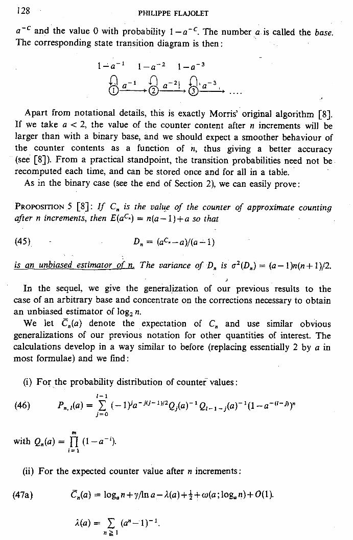
I28 PHILIPPE FLAJOLET

a-' and the value 0 with probability 1 -a". The number a is called the base. The corresponding state transition diagram is then :

Apart from notational details, this is exactly Morris' original algorithm [SI. If we take a < 2, the value of the counter content after n increments will be larger than with a binary base, and we should expect a smoother behaviour of the counter contents as a function of n, thus giving a better accuracy (see [SI). From a practical standpoint, the transition probabilities need not be recomputed each time, and can be stored once and for all in a table.

As in the binary case (see the end of Section 2), we can easily prove:

PROPOSITION .5 [SI: r f C, is the value of the counter of approximate counting after n increments, then E(acn) = n(a- l ) + a so that

is an unbiased estimator of n. The variance of D, is 02(D,) = (a - l ) n ( n + 1)/2.

In the sequel, we give the generalization of our previous results to the case of an arbitrary base and concentrate on the corrections necessary to obtain an unbiased estimator of log, n.

We let c,,(a) denote the expectation of C, and use similar obvious generalizations of our previous notation for other quantities of interest. The calculations develop in a way similar to before (replacing essentially 2 by a in most formulae) and we find:

J

'

(i) For the probability distribution of counter' values : I - 1

~ , , ~ ( a ) = C (- l Y a - j ( j - 1 ) / 2 Qj (a) - QI - - j(a)-l(l - a-('-J')" j = O

(46)

m with Q,(a) = n ( l - a - i ) .

i = l

(ii) For the expected counter value after n increments:

(47a) C,(a) = log, n + ?/in a- A(a)+++ o ( a ;log, I?)+ O(1).

L(a) = c (a"- l ) - l . n r l

I I

i

~

I

i

i

I

~

I

I

I

APPROXIMATE COUNTING : A DETAILED ANALYSIS 129

a E(Xn )

2 10.001 13 2112 10.00307 2114 10.00712 2118 10.01 5 16 21/16 10.03027

(iii) For the standard deviation of the counter values:

(47b) o:(a) = o:(a)+x(u;log,n) +o(l), where ',

W

7 n

0.872 0.607 0.425 0.298 0.2 17

1 1 1 + - - - , 8 = 2x2/ lna .

2 n2 a" a,(a) = - -

.\. 'In2' ng1 ( ~ " - 1 ) ~ 12 ]nuk$, ksinh(6k)

-

2 2112

2114 2118 21/16

There follows from theke equations that for the content of the counter (with base a), the normalized value

7.01581 0.864 7.03 139 0.596

7.12340 0.276 7.23907 0.174

7.06266 0.409

(48) X = (C-K(a)).log,a where K ( a ) = y/lna- (a"-l)- '+$ n z l

is apart from negligible periodic fluctuations, an asymptotically unbiased estimator of log,n. The values K ( a ) for a = 2, 2112.. .21/16 are:

K(2) = - 0.2729 ; K(2'12) = - 2.8030 ; K(2"") = -9.8598 K(2"*) = -27.9714; K(2"I6) = -72.1936.

Figure 2 displays the expectations of X, (the value of the normalized variable X of (48) after n increments) for n =. 128, 1024 and a few values of a, together with the corresponding standard deviations of X, defined by:

4

' (49) 7,2(') = E ( ( X , - E(x">>2) .

Fig. 2. Bias and, accuracy of the normalized X value for sample values of a and n.

Table 2 shows that X is a very good estimate of log2n even for small values n (n - lo3). For smaller n (n - lo2) there is a slight bias which increases when a gets closer to 1. If necessary, corrections for smaller values of n could be easily tabulated using (47a) and introduced in the algorithm.

The accuracy of. that version of the algorithm is thus essentially determined by the dispersion of results it produces. The values of T,, for finite n are remarkably close to the asymptotic limit T,(u) = a,(a)/lna as shown by a cornparisan of

130 PHILIPPE FLAJOLET

results in Figure 2 with the values:

Thus to determine the effect of smaller bases on the accuracy of the algorithm, we only need to determine the dependence of 7,(a) on a. To do.so, it proves convenient, as we shall see, to study the behaviour of 7&2) as a + 1; this will lead to-very good numerical estimates on z,(a) for general a. From (47), we have:

+o(ln2a), a + 1. - 1 .’,(a) = (log, a) , [a -1 n z l ( a n - 1 ) 2

7r2

The asymptotics of the function appearing in the expression above

for small x are easily determined, again by Me11 the transform of c(x) is: I

so that, when x + 0:

n transform techniques since

c(x) - 1 Res(c*(s)x-’; a), CJ = 2, 1,0, - 1, ... . 0

~ ( x ) = (n2/6)x - - 2 - ’ x-l +O(l) . - -.

Thus, using this result in the expression of ~ ~ ( u ) :

6. Final conclusions.

We have examined in Section 5 , two possible ways of using the idea of approximate counting with a general base.

(i) The first one, which corresponds to Morris’ original algorithm, estimates n by. means of the random variable D defined by formula (45) and produces an unbiased estimate of n.

(ii) The second one estimates Iog,n by means of the random variable X

c

M

APPROXIMATE COUNTING A DETAILED ANALYSIS 131

defined by formula (48) and (apart from negligible fluctuations) leads to an asymptotically unbiased estimate of log, n.

As measures of tde accuracy of these algorithms, it is reasonable to consider: (i) The quotient betweedthe standard deviation of the estimate D and n,

which provides a measure of the relative accuracy of the algorithm. By Proposition 5, this ratio is asymptotic to

\ ’\

(ii) The standard deviation of the estimate X of log, n which from equation (50) is closely approximated by the function

The meaning of these formulas is probably best understood if we set a = 2l/” so that one gets better accuracy when rn gets large. Using approximations for large m, we find

pl (2llrn) - (In 2/2rn)’I2 ; p2(21/’”) - (rn In 4)- 1/2

(both approximations are fairly tight and for instance the approximation of pl is at most 3 % off the exact value of r , (a) for all m >= 1).

As. for the storage requirement of the aldgorithm, it is E(1+ hog, C , ] ) ; a quantity upper bounded by (and actually close to) 1 +log, E(C,), which by our previous results is itself close to log, log, n +log, m. Thus setting now 6 = log, rn we can roughly summarize the situation as follows : .

FACT. Using approximate counting with base a = 22-a one can count up to n using storage of about log, log, n + 6 bits; the accuracy of the results is close to 0.59 2-’12 and 0.85 2-6/2 respectively for the linear estimate algorithm (version ( i ) based on the variate D ) and for the logarithmic estimate algorithm (version ( i i ) based on the variate X ) .

As an example, consider taking as base a = 21/16 = 1.0 44...; such a confi- guration leads to an expected error on the estimate of log,n close to 0.2125. ff an unbiased estimate of n is sought using (45) the relative error given by (45) is typically less than 15%. This value of a makes it for instance possible to count up to about 65000 (216 = 65536) using 8 bits since log,(log, 216/10g, 2”16) = 8, and thus results in this particular case in halving the storage requirement of standard binary counters.

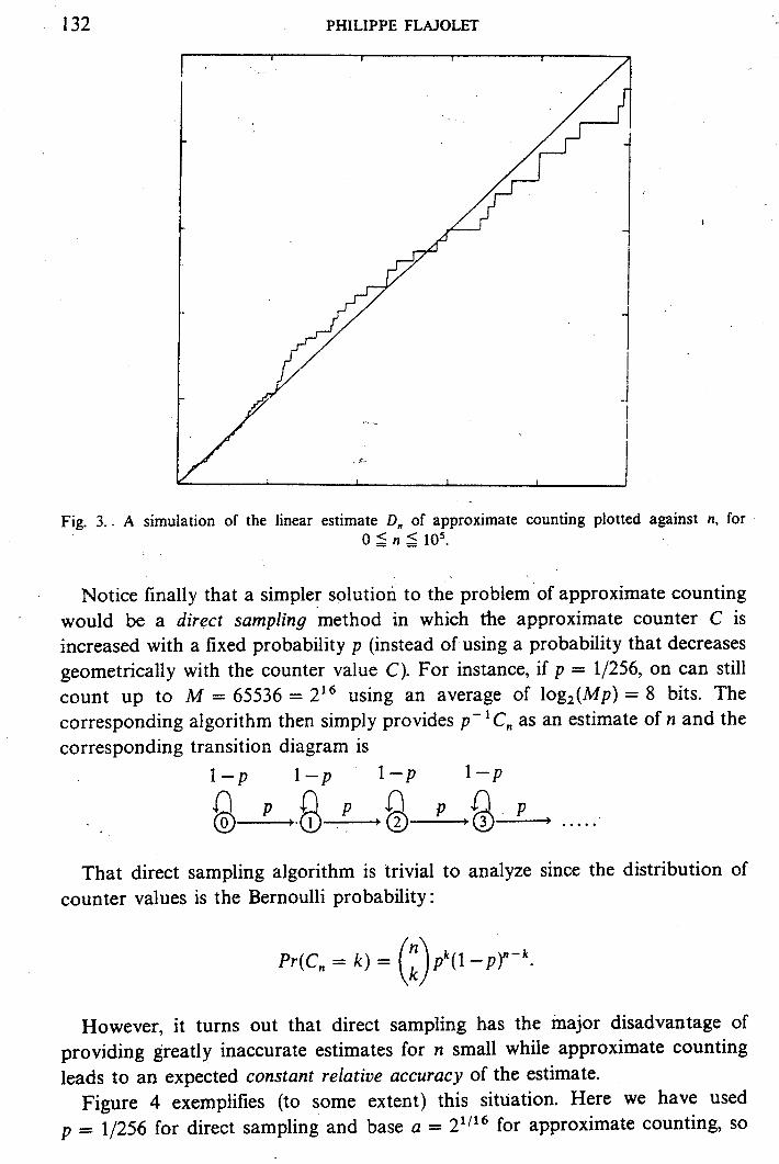
Figure 3 displays the result of a sample run of Approximate Counting with D, plotted against n for n = 0.. .lo5, using base a = 2’/16 and confirms the good behaviour of the algorithm.

132 PHILIPPE FLAJOLET

Fig. 3. - A simulation of the linear estimate D, of approximate counting plotted against n, for o 5 n 6 105.

. .

Notice finally that a simpler solution to the problem of approximate counting would be a direct sampling method in which the approximate counter C is increased with a fixed probability p (instead of using a probability that decreases geometrically with the counter value C). For instance, if p = 1/256, on can still count up to M = 65536 = 216 using an average of log,(Mp) = 8 bits. The corresponding algorithm then simply provides p - C, as an estimate of n and the corresponding transition diagram is

1 - P 1 - P 1-P 1 - P

That direct sampling algorithm is trivial to analyze since the distribution of counter values is the Bernoulli probability :

Pr(C, = k ) = (;)py* - - p r k .

However, it turns out that direct sampling has the major disadvantage of providing greatly inaccurate estimates for n small while approximate counting leads to an expected constant relative accuracy of the estimate.

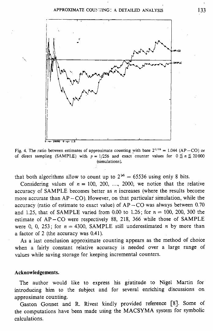
Figure 4 exemplifies (to some extent) this situation. Here we have used p = 1/256 for direct sampling and base a = 21/16 for approximate counting, so

.. ,

, \.

133 APPROXIMATE COUtCT'ING : A DETAILED ANALYSIS

I . I -I- ? .--

I

I I I -I- 2- 0 -y- 1.5

Fig. 4. The ratio between estimates of approximate counting with base 21'16 = 1.044 (AP-CO) or of direct sampling (SAMPLE) with p = 1/256 and exact counter values for 0 5 n 5 20000

(simulations).

that both algorithms allow to count up to 2"6 = 65536 using only 8 bits. Considering values of n = 100, 200, ..., 2000, we notice that the relative

accuracy of SAMPLE becomes better as n increases (where the results become more accurate than AP - CO). However, on that particular simulation, while the accuracy (ratio of estimate to exact value) of A P -CO was always between 0.70 and 1.25, that of SAMPLE varied from 0.00 to 1.26; for n = 100, 200, 300 the estimate of AP-CO were respectively 88, 218, 366 while those of SAMPLE were 0, 0, 253; for n = 4300, SAMPLE still underestimated n by more than a factor of 2 (the accuracy was 0.41).

As a last conclusion approximate counting appears as the method of choice when a fairly constant relative accuracy is needed over a large range of values while saving storage for keeping incremental counters.

Acknowledgements.

The author would like to express his gratitude to Nigel Martin for introducing him to the Subject and for several enriching discussions on approximate counting.

Gaston Gonnet and R. Rivest kindly provided reference [SI. Some of the computations have been made using the MACSYMA system for symbolic calculations.

134 PHILIPPE FLAJOLET

Recently K. Melhorn and K. Simon have shown the author some interesting connections of this work with the analysis of topological sorting under a random graph model; in particular they had obtained independently the first term in our expansion (47a).

BIBLIOGRAPHY

1. L. Comtet, t'Analyse Combinatoire, 2 vol., P.U.F., Paris (1970). 2. G. Doetsch, Handbuch der Laplace Transformation, Birkhauser Verlag, Base1 (1955). 3. P. Flajolet and N. Martin, Probabilistic counting, in Proc. 24th Annual Symp. on Foundations

4. R. G. Gallager, Variations on u theme by Huffmann, IEEE Trans. IT, 24 (1978) pp. 669-674. 5 . L. Kleinrock, Queuing Systems, Wiley Interscience, New York (1976). 6. D. E. Knuth, The Art of Computer Programming: Sorting and Searching, Addison-Wesley,

7. G. Langdon and J. Rissanen, Compression of black white images with binary arithmetic coding,

8. R. Morris, Counting large numbers of events in small registers, Comm. ACM, 21 (1978), pp.

9. S. Todd, N. Martin, G. Langdon and D,: Helman, Dynamic statistics collection for compression

10. E. T. Whittaker and G. N. Watson, A Course in Modern Analysis, (1907); 4th edition,

of Comp. Sc., Tucson, Arizona (1984), pp. 76-82.

Reading ( 1 973).

IEEE Trans. on Communications (1981).

840-842.

coding, Unpublished manuscript, 12 p. (1981).

Cam bridge Univ. Press, 1927.