Innovation Diffusion in Heterogeneous Populations:

Contagion, Social Influence, and Social Learning

By H. Peyton Young*

New ideas, products, and practices take time to diffuse, a fact that is often attributed to

some form of heterogeneity among potential adopters. This paper examines three broad

classes of diffusion models -- contagion, social influence, and social learning – and

shows how to incorporate heterogeneity into each at a high level of generality without

losing analytical tractability. Each type of model leaves a characteristic ‘footprint’ on

the shape of the adoption curve that provides a basis for discriminating empirically

between them. The approach is illustrated using the classic study of Ryan and Gross on

the diffusion of hybrid corn (JEL O33, D8, M3).

Keywords: diffusion, innovation, learning

*Department of Economics, University of Oxford, Manor Road, Oxford OX1 3UQ, U.K.

(email: peyton.young@economics.ox.ac.uk). I would like to thank Paul David, Steven

Durlauf, Joshua Epstein, Edoardo Gallo, James Heckman, Josef Hofbauer, Charles

Manski, David Myatt, Thomas Norman, Thomas Valente, Duncan Watts, Tiemen

Woutersen, and two anonymous referees for valuable comments on previous drafts.

Pierangelo de Pace and Jon Parker assisted with the data analysis. This research was

supported in part by The Brookings Institution and The Santa Fe Institute.

2

I. Models of innovation diffusion

A basic puzzle posed by innovation diffusion is why long lags occur between an

innovation’s first appearance and its general acceptance within a population. Among the

factors that have been suggested are delays in acting on information, a desire to conform,

learning from others, and changes in external factors such as prices. There is an

extensive literature on this phenomenon that spans economics, sociology, and marketing.1

Although the models are highly varied, a common theme is that delay results in part from

heterogeneity among potential adopters. People may realize different benefits and costs

from the innovation, or they may hear about it at different times, have different amounts

of information, different predispositions to conform, and so forth. Nevertheless, most of

the extant models incorporate heterogeneity in a very restricted fashion, say by

considering two homogeneous classes of agents, or by assuming that the heterogeneity is

described by a particular class of distributions.2

The purpose of this paper is three-fold. First, it will be shown that the benchmark models

in economics, marketing, and sociology proceed from fundamentally different

assumptions that lead to key differences in their dynamical structure. Second, each type

of model can be formulated at a high level of generality that allows for essentially any

distribution of heterogeneous characteristics without losing analytical tractability. Third,

each model leaves a distinctive ‘footprint’ in its pattern of acceleration that holds with

few or no restrictions on the distribution of characteristics. The reason is that they have

fundamentally different structures that details in the underlying distributions cannot

overcome.

1 For general overviews see Vijay Mahajan and Robert A. Peterson (1985), Mahajan, Eitan Muller, and Frank M. Bass (1990), Paul A.Geroski (2000), Paul Stoneman (2002), Everett M. Rogers (2003), and Thomas W. Valente (1995, 1996, 2005). 2 See in particular Abel Jeuland (1981), Richard Jensen (1982), Massoud Karshenas and Stoneman (1992), and Geroski (2000).

3

We shall consider three broad classes of models – contagion, social influence, and social

learning – that are drawn from the literature on marketing, sociology, and economics

respectively.3 The focus of attention will be on situations where the dynamics are driven

from within, that is, there are internal feedback effects from prior to future adopters.

Diffusion models that are driven mainly by external factors, such as price and quality

changes, obviously depend on the exogenous rates of change in these factors, so much

less can be said about them from an a priori standpoint.4

1. Contagion. People adopt when they come in contact with others who have already

adopted, that is, innovations spread much like epidemics.

2. Social influence. People adopt when enough other people in the group have adopted,

that is, innovations spread by a conformity motive.

3. Social learning. People adopt once they see enough empirical evidence to convince

them that the innovation is worth adopting, where the evidence is generated by the

outcomes among prior adopters. Individuals may adopt at different times due to

differences in their prior beliefs, amount of information gathered, and idiosyncratic costs.

Of the three categories of models, social learning is certainly the most plausible from an

economic standpoint, because it has firm decision-theoretic foundations: agents are

assumed to make rational use of information generated by prior adopters in order to reach

3 Some of these ideas have also been applied in anthropology; see in particular Robert Boyd and Peter J. Richerson (1985) and Joseph Henrich (2001). 4 These are sometimes called “moving equilibrium” models; see in particular David (1966, 1969, 1975, 2005), David and Trond E. Olsen (1984, 1986) and Stoneman (2002). There are also hybrid models in which the dynamics are driven by a combination of external and internal factors. The most common example is the Bass model, which will be considered in section 3.

4

a decision.5 By contrast, the contagion and social influence models are based on the

notion of exposure rather than on utility maximization. Why then should economists be

concerned with them? One reason is that they are the most prominent models in the

literature outside of economics, so it is worth understanding how they work in a general

setting. A second reason is that we would like to know whether adoption curves

generated by social learning differ from those generated purely by exposure, that is,

whether we can distinguish empirically between the two explanations.

We shall find that under certain conditions this is indeed the case. To make progress on

this question, however, we need to formulate the aggregate dynamics of each class of

model at a high level of generality without making restrictive assumptions about the

distribution of individual characteristics. This is particularly challenging in the case of

social learning models, where there are multiple sources of heterogeneity, including

different costs of adoption, different prior beliefs, and different amounts of information-

gathering. It turns out that all of these considerations can be folded together in a simple

dynamical equation that is easy to analyze.

One limitation of the analysis is the use of a “mean-field” approach in which the

population is assumed to be infinitely large and encounters between individuals are

purely random. If the population is finite and agents interact through a fixed social

network, the aggregate dynamics are substantially more complex and may depend on the

topology of the network. The extent to which our results can be generalized to this case is

an interesting question that will be left to future work.6

5 There is a large literature on social learning but the specific assumptions are highly varied . See among others Sushil Bikchandani, David Hirshleifer, and Ivo Welsh (1992), Abhijit Banerjee (1992), Alan Kirman (1993), Glenn Ellison and Drew Fudenberg (1993, 1995), Sandeep Kapur (1995), Venkatesh Bala and Sanjeev Goyal (1998), Lones Smith and Peter Sorensen (2000), Kalyan Chatterjee and Susan H. Xu (2004), Banerjee and Fudenberg (2004), and Charles F. Manski (2004). However, relatively little prior work has been done on the implications of social learning for the shape of the adoption curve. Notable exceptions are Henrich (2001), Jensen (1982), and Dunia Lopez-Pintado and Duncan J. Watts (2008). 6 For models of diffusion in social networks see Lawrence E. Blume (1993, 1995), Bala and Goyal (1998), H. Peyton Young (2003), Chatterjee and Xu (2004), Robin Cowan and Nicholas Jonard (2004), Matthew

5

The main results on shape and acceleration patterns can be summarized as follows.

1. A process that is driven purely by inertia must decelerate from start to finish, that is,

the adoption curve is strictly concave. Acceleration -- in particular S-shaped curves --

cannot be explained solely by delay no matter how the rates of inertia are distributed in

the population.7

2. A process that is driven purely by contagion typically accelerates initially and then

decelerates as it approaches saturation (the curve is S-shaped), but it cannot accelerate

beyond the fifty percent adoption level. When everyone is alike, the hazard rate (the rate

at which non-adopters become adopters) is linear and increasing in the current number of

adopters. From this it follows that the hazard rate must be non-increasing relative to the

number of adopters. Less obviously this result holds for any joint distribution of

‘infection’ rates from a combination of internal and external sources. This forms a

significant and testable implication of the contagion model, as we shall see in section 6.

3. A process that is driven purely by social influence can either decelerate or accelerate

initially, but in the latter case it typically accelerates at a super-exponential rate for some

period of time.

4. A process that is driven purely by learning from the experiences of others (social

learning with direct observation) usually begins slowly and may even decelerate initially.

If such a process does eventually accelerate, it typically does so at a super-exponential

rate for some period of time. Moreover, the overall rate at which adoption proceeds is a

monotone increasing function of the expected payoffs from adoption.

O. Jackson and Brian W. Rogers (2007), Jackson and Leeat Yariv (2007), Benjamin Golub and Jackson (2008), and Fernando Vega-Redondo (2007). 7This feature of inertia models distinguishes them from contagion models, as was pointed out in the classic study of medical innovation by James S. Coleman, Elihu Katz, and Herbert Menzel (1957, 1966). It is also a well-known feature of heterogeneous duration models (Tony Lancaster and Stephen Nickell, 1980; James J. Heckman and Burt Singer, 1982; Heckman, Richard Robb, and James R. Walker, 1990). We draw attention to it here because it shows in a particularly transparent way how restrictions on shape can hold irrespective of the distribution of individual characteristics (in this case the inertia rates).

6

These results provide a general framework for assessing the relative plausibility of

different mechanisms that could be driving a given diffusion process. It is not an

identification strategy, which is virtually impossible with aggregate-level data and

difficult enough with micro-level data. Rather, our results establish restrictions on the

shape of adoption curves that are associated with particular explanatory mechanisms.

The overall plausibility of a given explanation should be examined in conjunction with

other information about the specific nature of the process, e.g., whether it was driven

largely by internal communication among members of a population or by external

sources such as advertising campaigns, whether payoffs played a prominent role (as in

new production methods), or conformity was the main motive (as in new fashions). We

outline how this framework can be applied empirically using Bryce Ryan and Neal C.

Gross’s classic study of the diffusion of hybrid corn in the 1920s and 1930s (Ryan and

Gross, 1943). While the data in this study are rather limited, it illustrates how the

approach can be brought to bear on actual cases, and also highlights the kinds of data that

one would need to conduct a full-fledged empirical analysis.

II. Inertia

Before launching into a discussion of the three main models, it will be useful to consider

a much simpler reason why innovations take time to diffuse, namely, people sometimes

delay in acting on new information. This hypothesis leads to a particularly tractable

model that has been studied in other contexts, notably heterogeneous duration models

(see among others Lancaster and Nickell, 1980; Heckman and Singer, 1982; Heckman,

Robb, and Walker, 1990). We include it here because it forms a useful foil for the

models to come later; furthermore all of the other models include inertia as one of the

parameters, so this is by far the simplest case to analyze.

First, consider a model of delayed adoption in which there is no heterogeneity among the

agents. Let λ > 0 be the instantaneous rate at which any given non-adopter first adopts.

7

Let ( )p t be the proportion of adopters at time t , and let us set the clock so that (0) 0p = .

The function ( )p t is called the adoption curve. Assume for simplicity that once agents

have adopted the new technology, they do not switch back to the old technology within

the time frame of the analysis. Then the expected motion is described by the ordinary

differential equation ( ) (1 ( ))p t p tλ= − , which has the solution ( ) 1 tp t e λ−= − given the

initial condition (0) 0p = .

Notice that this curve is concave throughout; in particular, it is not S-shaped. It is a rather

remarkable fact that this remains true when any amount of heterogeneity is introduced.

To see this, suppose that ( )ν λ is the distribution of λ in the population. Then the

expected trajectory of the process is given by

(1) ( ) 1 tp t e dλ ν−= − ∫ .

Differentiating (1) twice over, we see that ( ) 0p t < irrespective of the distribution ( )ν λ .

The intuition is straightforward: agents with high values of λ tend to adopt earlier than

those with low values of λ . It follows that the average value of λ in the current

population of non-adopters is non-increasing, and the number of such individuals is

strictly decreasing. Thus the flow of new adopters is strictly decreasing.

This simple example illustrates the kinds of results that hold in more complex situations:

the structure of the model has implications for the shape of the curve that remain true

even when an arbitrary amount of heterogeneity is introduced.

III. Contagion

Contagion refers to a process in which people adopt a new product or practice when they

come in contact with others who have adopted it. An everyday example would be a new

fashion that spreads because people imitate those who have already adopted. The

8

resulting dynamics are similar to those of an epidemic; indeed, some of the models are

borrowed directly from the epidemiology literature. In the context of innovation

diffusion it is common to use a two-parameter model that allows for contagion from

within the group at one rate, and from sources outside the group at a different rate. This

is known as the Bass model of new product diffusion (Bass, 1969, 1980) or the mixed-

influence diffusion model (Mahajan and Peterson, 1985). In the context of a new fashion

in clothing, for example, these two rates would correspond to seeing other people on the

street who are wearing it, and seeing television ads that promote it.8

Let us begin by describing the homogeneous version of the model, later we shall

introduce heterogeneity. Let λ be the instantaneous rate at which a current non-adopter

‘hears about’ the innovation from a previous adopter within the group, and let γ be the

instantaneous rate at which he ‘hears about’ it from sources outside of the group. We

shall assume that λ and γ are nonnegative, and that not both are zero. In the absence of

heterogeneity, such a process is described by the ordinary differential equation

( ) ( ( ) )(1 ( ))p t p t p tλ γ= + − , and the solution is

(2) ( ) ( )( ) [1 ] /[1 ]t tp t e eλ γ λ γβγ βλ− + − += − + , 0λ > .

When contagion is generated purely from internal sources ( 0γ = ) this boils down to the

ordinary logistic function, which is of course S-shaped.9 When innovation is driven

solely by an external source ( 0γ > and 0λ = ), we obtain the pure inertia discussed

earlier. When both γ and λ are positive, we can choose β in expression (2) so that

(0) 0p = ; namely, with 1/β γ= we obtain

(3) ( ) ( )( ) [1 ] /[1 ( ) ]t tp t e eλ γ λ γλ γ− + − += − + / .

8 Some forms of internet advertising attempt to exploit internal feedback effects by informing members of a target group how many other members of their group have already adopted.

9

This model has spawned many variants, some of which assume a degree of heterogeneity,

such as two groups with different contagion parameters (Karshenas and Stoneman, 1992;

Geroski, 2000), while others employ distributions from a specific parametric family, such

as gamma distributions (Jeuland, 1981).

In fact, we can formulate a fully heterogeneous version that is analytically tractable and

places virtually no restrictions on the joint distribution of the parameters. Specifically,

let μ be the joint distribution of the contagion parameters λ and γ . Assume for

analytical convenience that μ has bounded support, which we may take to be 2[0,1]Ω = .

(Rescaling λ and γ by a common factor is equivalent to changing the time scale, so this

involves no real loss of generality.) The only substantive restriction that we shall place

on μ is that, averaged over the whole population, external influence is positive

( 0dγ γ μΩ

= >∫ ), for otherwise the process cannot get out of the initial state (0) 0p = .

Let ( )p tλ γ, be the proportion of all type- ( )λ γ, individuals who have adopted by time t .

Then the proportion of all individuals who have adopted by time t is

(4) ( ) ( )p t p t dλ γ μ,= ∫ .

(Hereafter integration over Ω is understood.) Each subpopulation of adopters ( )p tλ γ,

evolves according to the differential equation

(5) ( ) ( ( ) )(1 ( ))p t p t p tλ γ λ γλ γ, ,= + − .

9 The logistic model was common in the early work on innovation diffusion; see for example Zvi Griliches (1957) and Edwin Mansfield (1961).

10

This defines an infinite system of first-order differential equations coupled through the

common term ( )p t . We can reduce it to a single differential equation by the following

device: let ( ) ln(1 ( ))x t p tλ γ λ γ, ,= − and observe that (5) is equivalent to the

system ( ) ( ( ) )x t p tλ γ λ γ, = − + for all ( )λ γ, . From this and the initial condition

(0) 0xλ γ, = we obtain

(6) t

0 0( ) ( ( ) ) ( )

tx t p s ds p s ds tλ γ λ γ λ γ, = − + = − −∫ ∫ .

From the definition of ( )x tλ γ, it follows that

(7) ( )

( ) 1x t

p t e dλ γ μ,= − ∫ ,

that is, ( )p t satisfies the integral equation

(8) 0( )

( ) 1t

t p s dsp t e d

γ λμ

− − ∫= − ∫ .

In other words, the current number of nonadopters 1 ( )p t− decays according to a

weighted average of exponential functions, where the exponent depends on the elapsed

time t and the average adoption level up to t. Starting from the initial condition

(0) 0p = , one can solve for ( )p t by successive approximation.

In this model the hazard rate ( ) /(1 ( ))p t p t− may be increasing or decreasing depending

on the relative importance of the internal and external sources of contagion. It turns out,

however, that the hazard rate cannot increase relative to the current number of adopters,

that is, the ratio ( ) /[ ( )(1 ( ))]p t p t p t− must be nonincreasing. Furthermore, if contagion

from external sources is present, the ratio must be strictly decreasing. We shall call this

ratio the relative hazard rate.

11

When the parameters λ γ, are fixed, it is obvious that that the relative hazard rate is

nonincreasing, indeed this follows at once from the equation ( ) ( ( ) )(1 ( ))p t p t p tλ γ= + − .

The claim is not so obvious when the parameters are heterogeneously distributed,

including the possibility that λ and γ are negatively correlated: people who are heavily

influenced by outside sources (high γ ) might be less susceptible to information from

inside sources (low λ ), and so forth.

Proposition 1. Suppose that diffusion is driven by heterogeneous contagion with positive

external influence. Then the hazard rate decreases relative to the number of adopters,

which implies that the process cannot accelerate beyond 1/ 2p = .

The last statement follows immediately from the prior one, because if ( )p t were to

accelerate beyond ½, then at that point the numerator of ( ) /[ ( )(1 ( ))]p t p t p t− would be

increasing and the denominator would be decreasing, contradicting the assertion that the

hazard rate decreases relative to the number of adopters (this is proved in the Appendix).

We remark that there are perfectly reasonable S-shaped curves that do not satisfy the

monotonicity condition in proposition 1. Consider, for example, an adoption process

described by the differential equation ( ) ( )(1 ( ))ap t p t p t= − , which was first proposed as

a model of innovation diffusion by Christopher J. Easingwood, Mahajan, and Muller

(1981, 1983). When 1a > , 1( ) /[ ( )(1 ( )] ( )ap t p t p t p t−− = is strictly increasing, hence

Proposition 1 shows that such a process cannot arise from a contagion model with any

amount of heterogeneity. Nevertheless, it is possible to generate an S-shaped curve from

a contagion model -- in fact from a homogeneous contagion model – whose overall

appearance is very similar (see Figure 1).

12

0

0.1

0.2

0.3

0.4

0.5

0.6

0.7

0.8

0.9

1

0 2 4 6 8 10 12 14 16 18 20 Figure 1. Two adoption curves: the solid line is generated by 1.1( ) (1 )p t p p= − and

(0) 0.01p = , the dashed line by a Bass model with .75λ = and .0025γ = . IV. Social influence

The sociological literature on innovation stresses the importance of social pressure on

individual decisions about whether to adopt. In the standard model individuals are

assumed to have different ‘thresholds’ that determine whether they will adopt as a

function of the number (or proportion) of others in the population who have already

adopted. The dynamics of these models were first studied by Thomas C. Schelling

(1971, 1978), Mark Granovetter (1978), and Granovetter and Roland Soong (1988); for

more recent work in this vein see Michael W. Macy (1991), Valente (1995, 1996, 2005),

Peter Sheridan Dodds and Watts (2004, 2005), Damon Centola (2006), and Lopez-

Pintado and Watts (2008).

For each agent i , suppose that there exists a minimum proportion 0ir ≥ such that i

adopts as soon as ir or more of the group has adopted. (If 1ir > the agent never adopts.)

This is called the social threshold of agent i . The precise meaning of these thresholds

varies from one context to another; broadly speaking we can think of them as degrees of

responsiveness to social influence. A concrete example would be the transmission of

rumors: some people would need to hear the rumor from many people to pass it on while

others might only need to hear it once. Another is fashion: some people need to see only

a few others wearing a new kind of clothing in order to try it, whereas others will wait

13

until the fashion is widespread before jumping on the bandwagon. A key feature of such a

model is that the adoption depends on the innovation’s current popularity rather than on

how good or desirable the innovation has proven to be.10 The latter is the basis of social

learning models, which we shall take up in the next section.

We wish to model the aggregate dynamics without assuming a specific parametric form

for the distribution of thresholds. To this end, let ( )F r be the cumulative distribution

function of thresholds in some given population. At time t the proportion of people

whose thresholds have been crossed is ( ( ))F p t . Of these, ( )p t have already adopted, so

the proportion whose thresholds have been crossed but have not yet adopted is

( ( )) ( )F p t p t− . Let 0λ > be the instantaneous rate at which these people convert. Then

the adoption process is described by the differential equation

(9) ( ) [ ( ( )) ( )], 0p t F p t p tλ λ= − > .

Assume that (0) 0F > and let b be the first fixed point of F , that is, the smallest number

in (0, 1] such that ( )F b b= , if any such exists; otherwise let 1b = . We then have

( )F p p> for all [0, )p b∈ . Since (9) is a separable ordinary differential equation, we

obtain the following explicit solution for the inverse function 1( )t p x−= :

(10) [0, ),x b∀ ∈ 1

0( ) (1/ ) /( ( ) )

xt p x dr F r rλ−= = −∫ .

Notice that the right-hand side is integrable because ( )F r is monotone nondecreasing

and ( )F r r− is bounded away from zero for all r in the interval [0, ]x whenever x b< .

(The constant of integration is zero because of the initial condition (0) 0p = .) As x b→ ,

the right-hand side of (10) goes to infinity, which implies that the adoption curve

10Popularity is a factor in some of the economics models of diffusion; see in particular Ellison and Fudenberg (1993, 1995).

14

approaches b asymptotically. In particular, the adoption process peters out as it

approaches the first fixed point of F .

This phenomenon is illustrated in figure 2. Here we assume that the thresholds are

normally distributed to the right of the origin, and there is a point mass at the origin

corresponding to the subset of innovators -- the people who are willing to adopt even

when no one else adopted. Notice that the adoption curve asymptotes to 0.50p = ,

which is the first fixed point of F . There is nothing special about the normal distribution

in this regard; similar results hold for any c.d.f. where it first crosses the 45o - line.

The adoption curve in figure 2 is concave, but this is by no means necessary or even

typical for this family of models. Figure 3 illustrates an entirely different adoption curve

that is generated by a truncated normal with smaller mean and variance. An interesting

feature of this curve is that it accelerates very sharply in the early stages; indeed it can be

shown that it grows at a faster-than-exponential rate up to 0.10p = .

We claim that whenever the process starts in the left tail of the distribution the curve must

have one of two shapes: either it decelerates initially, or it accelerates initially at a super-

exponential rate. To see why this is so, consider the basic dynamic equation in (9).

Assume that (0) 0F > and that F has a continuous density ( )f p defined for all

(0,1]p ∈ . (Note that the density is not defined at the origin because there is a point mass

there.) Differentiating (9) with respect to t and dividing through by ( )p t , which by

assumption is positive, we obtain

(11) ( ) / ( ) [ ( ( )) 1]p t p t f p tλ= − .

In other words, the relative acceleration rate traces out a positive linear transformation of

the underlying density. It follows that the process accelerates initially if and only if the

initial density is large enough, that is, ( ) 1f p > in a neighborhood of the origin. Suppose

15

0

0.2

0.4

0.6

0.8

1

1.2

-1.5 -1 -0.5 0 0.5 1 1.5 2 2.5

r

f(r)

a) truncated normal density of thresholds

0

0.2

0.4

0.6

0.8

1

1.2

0 0.5 1 1.5 2 2.5

r

F(r)

b) c.d.f. of thresholds and 45o - line

0

0.2

0.4

0.6

0.8

1

1.2

0 1 2 3 4 5

t

p(t)

c) social threshold adoption curve ( )p t Figure 2. Density, c.d.f., and social threshold adoption curve generated by N(.50, .25) and λ = 4.

16

0

0.5

1

1.5

2

2.5

3

3.5

4

4.5

-0.3 -0.2 -0.1 0 0.1 0.2 0.3 0.4 0.5 0.6 0.7

r

f(r)

a) truncated normal density of thresholds

b) c.d.f. of thresholds and 45o - line

0

0.2

0.4

0.6

0.8

1

1.2

0 0.25 0.5 0.75 1 1.25 1.5 1.75 2

t

p(t)

c) social threshold adoption curve ( )p t Figure 3. Density, c.d.f., and social threshold adoption curve generated by N(.10, .01) and λ = 4.

17

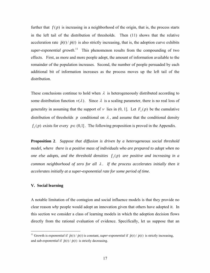
further that ( )f p is increasing in a neighborhood of the origin, that is, the process starts

in the left tail of the distribution of thresholds. Then (11) shows that the relative

acceleration rate ( ) / ( )p t p t is also strictly increasing, that is, the adoption curve exhibits

super-exponential growth.11 This phenomenon results from the compounding of two

effects. First, as more and more people adopt, the amount of information available to the

remainder of the population increases. Second, the number of people persuaded by each

additional bit of information increases as the process moves up the left tail of the

distribution.

These conclusions continue to hold when λ is heterogeneously distributed according to

some distribution function ν λ( ) . Since λ is a scaling parameter, there is no real loss of

generality in assuming that the support of ν lies in (0, 1]. Let ( )F pλ be the cumulative

distribution of thresholds p conditional on λ , and assume that the conditional density

( )f pλ exists for every (0,1]p ∈ . The following proposition is proved in the Appendix.

Proposition 2. Suppose that diffusion is driven by a heterogeneous social threshold

model, where there is a positive mass of individuals who are prepared to adopt when no

one else adopts, and the threshold densities ( )f pλ are positive and increasing in a

common neighborhood of zero for all λ . If the process accelerates initially then it

accelerates initially at a super-exponential rate for some period of time.

V. Social learning

A notable limitation of the contagion and social influence models is that they provide no

clear reason why people would adopt an innovation given that others have adopted it. In

this section we consider a class of learning models in which the adoption decision flows

directly from the rational evaluation of evidence. Specifically, let us suppose that an

11 Growth is exponential if ( ) / ( )p t p t is constant, super-exponential if ( ) / ( )p t p t is strictly increasing, and sub-exponential if ( ) / ( )p t p t is strictly decreasing.

18

agent adopts if he has reason to believe the innovation is better than what he is doing

now, where the evidence comes from directly observing the outcomes among prior

adopters. For example, when a new product becomes available -- e.g., a new type of

medication (antibiotics) or a new communication technology (cellphones) -- people will

want to see how it works for others over a period of time before trying it themselves.

These are variously known as social learning models or social learning models based on

direct observation.

There is a sizable theoretical literature on social learning, but it is difficult to summarize

due to the great diversity in behavioral and informational assumptions that different

authors use. Some assume that payoff outcomes among prior adopters are fully

observable, while others assume only that the act of adoption is observable (the latter are

usually called herding models). Some assume that agents can recognize others’ types,

while others assume that types cannot be identified. There are also significant differences

in the relevant characteristics that authors choose to focus on, including heterogeneity in

risk aversion, discount rates, and amount of information.12 There is considerable

empirical evidence, however, that learning from the experience of others does in fact

occur.13

Here we shall make a number of simplifying assumptions in order to get a handle on an

issue that has not received much previous attention in this literature, namely, what do the

short-run aggregate dynamics of a heterogeneous learning model look like, and do they

differ qualitatively from the dynamics generated by other classes of models?

To make some progress on this question let us make the following assumptions: i)

payoffs are observable; ii) payoffs generated by different individuals and/or at different

points in time are independent and equally informative; iii) agents are risk-neutral and

12 See among others Bikchandani, Hirshleifer, and Welsh (1992), Banerjee (1992), Kirman (1993), Ellison and Fudenberg (1993, 1995), Kapur (1995), Bala and Goyal (1998), Smith and Sorensen (2000), Chatterjee and Xu (2004), Banerjee and Fudenberg (2004), Manski (2004), Golub and Jackson (2008). 13 Andrew Foster and Mark Rosenzweig (1995), Kaivan Munshi (2004), Timothy G. Conley and Christopher R. Udry (2005).

19

myopic; iv) there is no idiosyncratic component to payoffs due to differences in agents’

types, but agents may have different costs (not necessarily observable); v) there are

differences in agents’ prior beliefs about how good the innovation is relative to the status

quo; vi) there are differences in the average number of people they observe and hence in

the amount of information they have; vii) the population is fully mixed. Many other

complicating factors could be introduced, such as discounting, one-time switching costs,

risk aversion, imperfect observability, restricted information acquisition (such as through

social networks), but these extensions would distract from the main point, which is to

identify the dynamic characteristics of a fairly general class of learning models without

attempting to formulate the most general such model.

We claim that, under the above assumptions, the dynamical system has a surprisingly

simple structure. One can reduce the various types of heterogeneity to a composite index

that measures the probability of a given agent adopting, conditional on the amount of

information that has been generated thus far in the population. The equation of motion

of such a process turns out to be analogous to the one obtained for the social influence

model, except that here the relevant state variable at time t turns out to be the integral of

the adoption curve up through t , 0

( )tp s ds∫ , rather than the level of adoption ( )p t .14 The

reason is that 0

( )tp s ds∫ measures the cumulative information generated by all prior

adopters from the time they first adopted, which is the relevant variable in the learning

context.

To illustrate how such a model works, let us walk through a particular example using a

standard normal-normal updating framework. This is chosen mainly for its

computational transparency; similar results hold under alternative assumptions.15

Assume that the payoff from the innovation is a normally distributed random variable X

14 Recall that the integral of the adoption curve also featured in the heterogeneous contagion model (see equation (8)). 15 Jensen (1982) and Lopez-Pintado and Watts (2008) study the case where the outcome variable is binomial (payoffs are “high” or “low”). They assume that agents pay attention only to current outcomes, not the cumulative amount of information generated from earlier periods.

20

with mean 0μ > and variance 2σ , which is i.i.d. among agents and time periods. We

shall interpret μ as the mean payoff gain per period from using the innovation as

compared to the status quo technology. Each agent is assumed to have an idiosyncratic

variable cost ic of using the innovation, so he adopts if and only if he believes that the

mean payoff per period is at least ic (thus he may switch back if after receiving more

information he believes that the mean payoff is less than ic ).

If everyone knew the true value of μ from the outset, then everyone would adopt for

whom ic μ< . This is the efficient outcome. Ex ante, however, people do not know the

true value of μ ; furthermore, they may start with substantially different beliefs (based on

their prior private information) about what the true value is. As more information comes

in, they update their beliefs. If this information is sufficiently favorable, more people

will adopt, which creates a still-larger base of information, which causes even more

people to adopt, and so on. This is the essential logic driving the learning dynamics.

To continue with our example, suppose that each agent i has a prior belief about the

unknown mean μ and unknown precision 21/ρ σ= such that: i) the marginal of ρ is

gamma-distributed, and ii) for each value of ρ the conditional distribution of μ is

normal with mean 0iμ and precision iρτ . (This is a standard normal-normal updating

model; see Morris De Groot (1970).) Low values of iτ reflect flexibility in beliefs, that

is, relatively little evidence is needed to shift 'i s belief about the mean by a given

amount. Low values of 0iμ reflect pessimism about the payoffs from the innovation. In

particular, if i initially believes that the mean is less than his costs, 0i icμ < , he will not

want to adopt. As more information comes in, however, his posterior estimate of the

mean, itμ , may increase sufficiently that he changes his mind. The point at which this

happens depends, among other things, on how much information i collects and how

flexible his beliefs are.

21

At a given point in time t , agent i will have seen (or heard about) a random assortment

of prior outcomes depending on the chance encounters he had with other members of the

population. In a continuous-time setting the total “number” or measure of prior outcomes

up to time t is given by the integral under the adoption curve, namely, 0

( ) ( )t

r t p s ds= ∫ .

Assuming that i is equally likely to see any particular outcome, we can model 'i s flow

of information by a Poisson arrival process. In particular, let itN be a Poisson random

variable representing the number of 'i s observations up to time t , where [ ] ( )it iE N r tβ=

and the parameter iβ is a measure of the extent to which i “gets around.”16

Let itn denote the realization of itN , and let itx denote the mean payoff among these itn

observations. Given our assumptions, itx is normal with mean μ and standard deviation

/ itnσ . In the normal-normal updating framework, 'i s Bayesian posterior estimate of

the mean, itμ , can be expressed very simply as a convex combination of 0iμ and itx ,

namely,

(12) 0it it i iit

it i

n xn

τ μμτ

+=

+ .

In other words, the posterior estimate is just a weighted average of the prior and the

observed mean, where the weight on the mean is the number of independent observations

that produced it.

Given our assumption that i is myopic, she is prepared to adopt once itμ is at least equal

to her variable ic , which by (12) is equivalent to

(13) 0( ) ( )it i it i i ix c n cτ μ− ≥ − .

16 If agents were embedded in a fixed social network, the analogous parameter would be the number of other agents with whom a given agent is connected. In this case, however, the aggregate amount of information ( )r t will generally not be sufficient to describe the state of the system; the dynamics of the process will depend on the specific network topology. See Golub and Jackson (2008).

22

By assumption ( )( / )it it itx n zμ σ− = is (0,1)N , hence (13) can be re-written as

(14) 0( ) ( )iti it i i i

it

z c n cn

σ μ τ μ+ − ≥ − .

To make sense of this expression, let us focus on the subpopulation of agents for whom

adoption is worthwhile, 0 { : }iP i cμ= > , and substitute the expected value [ ] ( )it iE n r tβ=

into (14). After rearranging terms we obtain

(15) 0 ( ))( )( )( ) ( )

iti i i

i i i i

r t zcr tc c

στ μβ μ μ β

−≥ −

− −.

Define 'i s resistance level (or information threshold) to be the expected value of the

right-hand side of this inequality, namely,

(16) 0( )( )

i i ii

i i

crc

τ μβ μ

−=

− .

We shall say that an agent is of type i if she has the vector of characteristics

( 0, , ,i i i ic τ β μ ). From (15) and (16) we see that an agent of type i is increasingly likely to

adopt as ( )r t passes the threshold ir . Moreover, this threshold has a natural

interpretation: agents with high ir are those who are initially pessimistic that the

innovation will cover their costs ( 0i ic μ− is large), inflexible in their initial beliefs ( iτ is

large), marginally profitable ( icμ − is low), and relatively uninformed ( iβ is small).

The precise form of expressions (15) and (16) is not essential for our purpose however:

the key point is that each agent i has a response function ( )i rφ , which represents the

23

probability that i believes the innovation is worth adopting, given that the total amount of

information generated by the prior adopters equals r .17

Let us now abstract from this particular example and take the notion of a response

function as a primitive of the learning model. Suppose that each agent in the population

has a “type” i that is characterized by a response function : [0,1]i Rφ + → , where ( )i rφ is

the probability that 'i s information threshold has been crossed when the total amount of

information generated by the prior adopters is r . For ease of interpretation we shall

assume that the functions ( )i rφ are monotone nondecreasing, though this is not actually

necessary for some of the results to follow. Notice that a given individual will typically

know only a small fraction of the prior outcomes, that is, r is a state variable that

represents a common pool of information but it is not common knowledge.

Assume that there are countably many types in the population, and let ip be the

proportion of i -types.18 When the total information generated by prior adopters equals

r , the proportion of the population whose thresholds have been crossed is given by the

function

(18) ( ) ( )i ii

F r p rφ= ∑ .

17 In the present case, the response function has the following explicit representation. Given that ( )r t r= ,

itn is Poisson-distributed with mean i rβ . Given a realization 0itn k= > , the mean observed payoff, itx ,

is normal with mean μ and variance 2 / kσ . Let Φ denote the standard normal c.d.f. Then the probability that 'i s posterior estimate exceeds 'i s costs, i.e., the probability that (13) holds, is

(17) 0

1

( ) ( ) ( )( ) [( ]

!

i rk

i i i i i

k

i

r e c k cr

k k

ββ μ τ μ

σ σφ

−∞

=

− −= Φ −∑ .

18 Alternatively we could assume that the types are uncountable and distributed according to a density; this makes no material difference in the subsequent analysis.

24

( )F r is a monotone nondecreasing function which we can interpret as a notional

distribution function of agents’ information thresholds. We allow for the possibility that

some agents have an infinite threshold, hence lim ( )r F r→∞ may be less than one. 19

Recalling  that 0

( ) ( )t

r t p s ds= ∫ , it follows that the aggregate dynamics is described by

the differential equation

(19) 0

( ) [ ( ( ) ) ( )], 0t

p t F p s ds p tλ λ= − >∫ .  

 

Observe that (19) is analogous to the dynamical equation (9) defining a social threshold

model, except that in the present case the argument of F is the integral of the adoption

curve rather than the adoption curve itself. This arises because agents use all past

information generated by previous adopters rather than just the most recent information.

Note that this formulation hinges on our assumption that payoff information is equally

informative no matter when it was received. If this were not the case, for example if

payoffs received in earlier time periods were less valuable, the defining equation would

have to be modified accordingly.20

The cumulative feature of the social learning model has some important implications for

the shape of the adoption curve. Compared to the social influence model acceleration is

initially quite weak; in fact in a neighborhood of the origin the process strictly

19 The closest model to this one in the literature is due to Dodds and Watts (2004, 2005). They consider a cumulative-dose model of infection with heterogeneity in the thresholds at which agents become infected (including social as well as biological interpretations of infection), though their analysis of the dynamics emphasizes different features from the ones considered here. 20 If payoff information is discounted at some rate 0δ > , the dynamical equation takes the form

( )

0( ) [ ( ( ) ) ( )]

t t sp t F e p s ds p tδλ − −= −∫ . Note that when δ is large, this process is similar to the social

influence model.  Another modification is to allow for joint heterogeneity in λ and r; this extension is straightforward and is left to the reader.

25

decelerates irrespective of the distribution generating it. To see why this is so,

differentiate equation (19) to obtain the acceleration equation

(20) (1/ ) ( ) ( ) ( ( )) ( )p t p t f r t p tλ = − .

By assumption (0) 0p = and the solution ( )p t is continuous, so the first term is close to

zero when t is close to zero. However, the second term is bounded away from zero when

t is close to zero, because (19) implies that (0) (0) 0p Fλ= > . Hence

(21) 20

lim ( ) (0) ( (0)) (0) 0t

p t F f p pλ+→= − + < .

More generally, when we compare (20) with the acceleration equation for the social

influence model, namely, (1/ ) ( ) ( ) ( ( )) ( )p t p t f p t p tλ = − , we see that the former has

weaker initial acceleration than the latter because ( )p t is initially positive whereas ( )p t

is initially zero. The result may be an extended period of weak growth in the early phases

of social learning. The reason is that the initial block of optimists (0)F exerts a

decelerative drag on the process: they contribute at a decreasing rate as their numbers

diminish, while the information generated by the new adopters gathers steam slowly

because there are so few of them to begin with.21 Figure 4 illustrates this phenomenon

for the same density that generated the social thresholds adoption curve in Figure 3.

21Initial deceleration does not necessarily occur, however, if observations are bunched at particular points in time. An example would be an agricultural innovation (e.g., a new type of crop) that is tried once in each growing season, and whose outcomes farmers observe at the end of the season. This case will be discussed further in section 6.

26

0

0.2

0.4

0.6

0.8

1

1.2

0 0.25 0.5 0.75 1 1.25 1.5 1.75 2

t

p(t)

Figure 4. Adoption curve generated by social learning, a normal distribution of

information thresholds N(.10, .01), and λ = 4.

Next we shall investigate the behavior of the relative acceleration rate ( ) / ( )p t p t . To

avoid uninteresting technical complications let us assume that the density is well-behaved

near the origin, that is, 0

(0) lim ( ) 0r

f f r+→= > , and that f ′ is continuous and bounded.

Define

(22) ( ) (1/ ) ( ) / ( )t p t p tφ λ= .

From (20) we deduce that

(23) ( ) ( ( )) ( ) / ( ) 1t f r t p t p tφ = − .

Differentiating (23) we obtain

(24) 2 2( ) ( ( )) ( ) / ( ) ( ( )) ( ( )) ( ) ( ) / ( )t f r t p t p t f r t f r t p t p t p tφ ′= + − .              

As 0t +→ the first term in (24) goes to zero, because by assumption f ′ is bounded,

( ) 0p t → , and (0) 0p > . The third term also goes to zero. However,

( ( )) (0) 0f r t f→ > , so the second term is positive in the limit. It follows from continuity

27

that ( )tφ is strictly positive on some initial interval 0 t T≤ ≤ . In the region near the

origin where ( ) 0p t < , this says that the relative acceleration rate is becoming less

negative.

Now suppose that at some time 0t the process begins to accelerate. If at this point the

density is increasing, then 0( ( )) 0f r t′ > , and it follows from (24) and continuity that ( )tφ

is positive for some interval of time beginning at 0t . In other words, if the density is

increasing when the process begins to accelerate (assuming it ever does accelerate), then

the process undergoes a period of super-exponential growth.

Proposition 3. Suppose that diffusion is driven by social learning, where there is a

positive mass of individuals who adopt even when no one else adopts ( (0) 0F > ), and the

distribution of resistances has a density ( )f r that is bounded away from zero near the

origin and has a continuous bounded derivative. Then initially the process decelerates

whereas the relative acceleration rate strictly increases. If the process begins to

accelerate, and if the density is increasing at that point, then the process undergoes a

period of super-exponential growth.

Propositions 2 and 3 show that both the social influence model and the social learning

model can exhibit periods of super-exponential growth. This is consistent with

observations by various authors that adoption curves often exhibit a sudden take-off

phase after a slow start (Ryan and Gross, 1943; Henrich, 2001; Maarten C. M. Vendrik,

2003; Rogers, 2003). The above propositions are more specific in predicting super-

exponential growth, and they clarify why one would expect it theoretically. Theory also

suggests why the curves generated by social influence and social learning will differ in

other respects. One difference is that, in a social learning model, the speed of adoption at

a given point in time depends on adoption levels at earlier points in time, whereas in a

social influence model this is not the case. Given sufficiently detailed adoption data this

effect could be tested by regression analysis with lagged variables.

28

A second distinction between the models is the way in which the resistance thresholds are

constructed. In a social influence model the thresholds reflect differences in a single

scalar parameter (people’s tendency to conform), whereas in a social learning model they

reflect differences in a variety of factors, including prior beliefs, amount of information

gathered, and the payoff gain from the innovation. Some of these factors are

unobservable and would be difficult estimate even with micro-level adoption data.

However, the payoff gain -- the parameter μ in the social learning model -- can

sometimes be estimated from the data, as we shall see the next section.

The key point to observe is that higher average payoffs from adoption shift the individual

response functions upward: for a given “number” of prior outcomes r in the population,

the probability ( )i rφ that any given individual i adopts increases the higher the potential

payoff gain μ . Thus if we consider two distinct populations { }1, 2 such that one has a

higher mean payoff than the other, say 2 1μ μ> , then all else being equal the resistance

distributions satisfy 2 1( ) ( )F r F r≥ for all r . ( 1F first-order stochastically dominates 2F .)

Under these circumstances, adoption occurs more rapidly in population 2 than in

population 1, that is, the solutions satisfy 2 1( ) ( )p t p t≥ for all t .22 This is one way to

evaluate the plausibility of the social learning model without knowing much about the

distribution of the learning parameters.

22 Consider the dynamical equations ( ) [ ( ( )) ( )], 1, 2i i i ip t F p t p t iλ= − = . Let 1 2( ), ( )p t p t be the solutions,

which we assume to be continuous. Note that 2 1(0) (0)p p≥ , because by assumption 2 1(0) (0)F F≥ and

1 2(0) (0) 0p p= = . Suppose, by way of contradiction, that 2 1( ) ( )p t p t< at some time 0t > . By

continuity there is a time 0t > such that 2 1( ) ( )p s p s≥ for all s t≤ and 2 1( ) ( )p t p t< . Therefore

2 10 0( ) ( )

t t

p s ds p s ds≥∫ ∫ and 2 2 1 10 0( ( ) ) ( ( ) )

t t

F p s ds F p s ds≥∫ ∫ , from which it follows that 2 1( ) ( )p t p t≥ , a

contradiction.

29

VI. The diffusion of hybrid corn

Diffusion data that permit definitive tests of the preceding propositions are not easy to

come by. One reason is that an adoption curve must be charted at frequent time intervals

in order to conduct tests of statistical significance. Consider, for example, a product or

practice that took ten years to go from introduction to completion. If the adoption level is

measured annually, there will be only ten data points, only nine first differences, and only

eight second differences; furthermore the errors in successive differences will not be

independent. Of course, the situation would be different if we had monthly or weekly

data over a period of ten years, but there appear to be very few data sets of this sort in the

literature. Moreover, the data that do exist tend to be for new products where mass

advertising played a critical role. In these cases it is difficult to sort out the relative

importance of internal and external sources of information, though the mixed-influence

contagion model is certainly a step in that direction.

Fortunately, there exist some data that are sufficiently detailed to carry out a preliminary

analysis of the ideas discussed above. The example we choose here is Ryan and Gross’s

classic study of the diffusion of hybrid corn in two Iowa communities (Ryan and Gross,

1943). This work prompted a number of later studies on innovation diffusion, including

Zvi Griliches’s analysis of hybrid corn diffusion across the midwestern and southern

United States (Griliches, 1957). Although the latter is more comprehensive in its

geographical coverage, the study by Ryan and Gross has several advantages for our

purposes. First, it was carried out at the community level, whereas the adoption curves

in Griliches’s study were aggregated over several counties and involved scores of

dispersed communities. Second, Ryan and Gross provided the proportion of hybrid corn

adopters, whereas Griliches gave the proportion of acreage planted in hybrid corn, which

(among other things) biases the results toward large landowners. Third, the Ryan and

Gross data covered the critical start-up phase in the 1920s, which was absent in

Griliches’s analysis. Finally, Ryan and Gross’s study included important related

information, such as the year that farmers first learned about the new technology and the

sources from which they learned about it. These data provide additional contextual

30

details that, together with the shape of the curve itself, allow us to assess the relative

plausibility of different diffusion mechanisms.

The adoption curve is shown in Figure 5. Particularly noteworthy features are the long

choppy start, which lasted for some six years (1927-32), followed by a sharp acceleration

for about four years (1933-36), and then a rapid deceleration as nearly 100 percent

acceptance levels were reached in 1941.23

Ryan and Gross repeatedly emphasize that natural conservatism was one of the key

reasons why farmers delayed so long in adopting a technology that could have

substantially increased their profits. Indeed, their survey data reveal that, although at

least two-thirds of the farmers had heard about the advantages of hybrid corn as early as

1931, only about 8 percent had adopted by then. Thus pure inertia could well have been

the explanation for the long delay. Nevertheless, the shape of the curve suggests that this

was not the case. The reason is that, in a pure inertia model with heterogeneous levels of

inertia, the adoption curve must be concave throughout. This hypothesis can be rejected

with reasonable confidence, since there was deceleration in only one of the first ten time

periods, and sharp acceleration in most of them. Thus, although inertia may have been a

contributing factor, it was unlikely to have been the sole factor.

Another interesting aspect of Ryan and Gross’s survey is that farmers reported their

sources of information about the new technology, and identified the sources they believed

were most influential in their decision to adopt. Whereas seed salesmen were listed as the

most common original source of knowledge, neighbors were listed as the most influential

in deciding whether to implement it. This is broadly consistent with the three classes of

models under consideration, all of which posit that adoption results from an internal

feedback loop between earlier and later adopters.

23 These features have been noted by other authors, notably Henrich (2001), who explains them by a combination of learning from direct experience and biased cultural transmission.

31

0.0 0.4 1.4 3.0 4.6 6.9 7.3 9.6 15.8 24.0 38.0 62.0 79.0 93.0 98.5 99.7 1926 1927 1928 1929 1930 1931 1932 1933 1934 1935 1936 1937 1938 1939 1940 1941

Figure 5. Percent of adopters of hybrid corn in two Iowa communities, 1926-41 (from Ryan and Gross, 1943, fig. 4).

Let us consider the contagion model first. This posits that adoption decisions are driven

by a combination of internal and external influences, where external influence operates at

a constant rate and internal influence operates at a rate proportional to the current number

of adopters. We know that this model generally produces S-shaped curves, but we also

know that the curve has a particular property: the hazard rate must be nonincreasing

relative to the current number of adopters. (It can be verified that this property also holds

in the discrete-time version.)

To check this, let tp be the proportion of adopters at the end of period t , and let

1t t tp p+Δ = − be the rate of change at t . Then / (1 )t t t tH p p= Δ − should be

nonincreasing in t , and strictly decreasing if there is any outside influence. tH is the

piecewise linear curve shown in figure 6.

To test whether it is monotone nonincreasing, let us fit a cubic polynomial using OLS

(the smooth line in figure 6).

32

2 31 2 3

1

2

0.034 (0.0034) 10.110.013 (0.0019) - 7.15

0.0018 (0.00029) 6.

tH a b t b t b t

abb

ε= + + + +

== −=

       coefficient                       t ‐ statistic

3

230.000069 (0.000013) - 5.48b = −

Figure 6. Cubic polynomial (smooth line) fitted by OLS to the relative hazard rate / (1 )t t t tH p p= Δ − (jagged line).

The overall fit is very good (R2 = .86), and the quadratic and cubic coefficients differ in

sign at a highly significant level. We therefore have reason to believe that tH is not a

monotone function, which is corroborating evidence against the contagion hypothesis.

Of course this is not the same as saying that there is no contagion effect, merely that this

effect by itself is unlikely to have produced the Ryan and Gross data.

Next let us consider the social influence and social learning models. Ryan and Gross

argued that the balance of evidence from the survey suggested some form of learning by

farmers: “In some sense the early acceptors provided a community laboratory from which

neighbors could gain some vicarious experience with the new seed over a period of some

years” (ibid, p. 16). This is precisely the effect posited in the social learning model. Is

social learning consistent with the shape of the curve? The answer is affirmative. Indeed

the curve has two features that are quite typical of social learning models: there is a long

33

slow start-up followed by very rapid acceleration. We remind the reader why this is so: in

the early phases adoption is driven mainly by people who are already convinced that the

new technology is a good idea but who may delay due to inertia; once this effect is

overcome there is rapid acceleration caused by the accumulation of information provided

by prior adopters, combined with the rising number of people at the margin who are

persuaded by the new information.

Unfortunately, the curve does not have enough data points to carry out tests of

significance, but we can make a rough estimate of the relative acceleration rate in the

following way. First compute the average slope over successive three-year intervals in

order to smooth out the data. Then compute the relative acceleration rate as the ratio of

successive slopes minus unity.24 The results are shown in table 1 for three different ways

of grouping the data. In every case the relative acceleration rate rises sharply from the

second to the third period. (Recall that in an exponential growth model the relative

acceleration rate would be constant.) While this is not proof of super-exponential

acceleration, it is certainly consistent with it.

These features provide corroborating evidence for social learning, but they certainly do

not constitute identification. For example, we cannot rule out the possibility that in the

mid-1930s there was an exogenous shock (e.g., a price war among seed companies) that

caused the sudden uptick.25 Moreover, the sharp rise in acceleration is equally consistent

with the social influence model. In this case, however, there is evidence from another

source – namely Griliches’s study – that social influence was probably not the sole

explanation. The reason is that, in a social learning model the rate of adoption depends on

the potential gain from adoption, whereas in a social influence model this is not the case.

One of Griliches’s main findings was that in the midwestern states generally (including

24 If tΔ is the slope in period t , then 1 1( ) / / 1t t t t t+ +

Δ − Δ Δ Δ Δ= − is an estimate of the relative acceleration rate at t . 25 It is worth noting, however, that Griliches investigated whether price changes in hybrid seed could explain the rates of adoption in various parts of the Midwest (including Iowa), and he found no significant effect (Griliches, 1957, p.503).

34

Iowa), the rate of adoption in each region was positively correlated with the estimated

monetary gain from adoption, just as the social learning model predicts.

Interval iΔ 1 / 1i i+Δ Δ − 1927-29 1.0 --

1930-32 1.4 1.4

1933-35 5.6 4.0

1936-38 18.3 3.3

1928-30 1.4 --

1931-33 1.7 1.2

1934-36 9.5 5.6

1937-39 18.3 1.9

1929-31 1.8 --

1932-34 3.0 1.7

1935-37 15.4 5.1

1938-40 12.2 0.8

Table 1. Relative acceleration rate measured over three-year intervals. iΔ is the average

annual change (in percent) over the ith interval, and relative acceleration is 1 / 1i i+Δ Δ − .

Putting all of this information together, we can say that social learning is consistent with

the observed pattern of diffusion of hybrid corn, although we cannot say that it was the

sole explanatory factor. However, we can also say with some confidence that inertia and

contagion were probably not the sole explanatory factors (and given Griliches’s findings

neither was social influence).

While the Ryan and Gross study is quite limited in scope, it highlights some of the issues

that would need to be addressed in a more complete empirical analysis. First, one would

need a curve – or set of curves -- that are measured at frequent time intervals. The reason

is that one requires an accurate estimate of the acceleration pattern at precisely the point

35

where acceleration is most rapid, hence frequent observations in this part of the curve are

crucial for running tests of significance. Second, one needs data that cover the whole

lifecycle of the adoption process, including the very early phases when adoption is just

getting started. Many of the data sets in the literature are quite weak in this respect; the

reason, of course, is that researchers are not likely to focus their attention on an

innovation until it is already well underway.

Third, the framework developed here applies to situations where there is informational

feedback between members of a group who interact more or less at random. If

information flows through a fixed network, say between individuals who are near

neighbors (in a geographical or social sense), then a different analysis will be required.

(Ryan and Gross did not say whether farmers learned more or less uniformly from others

in the community, or mainly from their immediate neighbors.) Fourth, we have restricted

our attention to social learning models in which people can directly observe outcomes

generated by other adopters. In the case of hybrid corn this assumption seems reasonable;

indeed Ryan and Gross specifically say that farmers looked at their neighbors’ fields to

assess the viability of the new technology (Ryan and Gross, 1943, p.16). In situations

where direct observation is not possible, one would need an analog of the theory in which

inferences are made indirectly.

Finally, the Ryan and Gross study highlights the importance of having supporting data

about the agents’ sources of information and the reasons they delayed in acting on it.

These contextual details, combined with an analysis of the shape of the curve, have the

potential to discriminate between alternative diffusion mechanisms even when detailed

micro-level data are unavailable.

36

REFERENCES

Bala, Venkatesh, and Sanjeev Goyal. 1998. “Learning from neighbours.” Review of

Economic Studies, 65: 595-621.

Banerjee, Abhijit. 1992. “A Simple Model of Herd Behavior.” Quarterly Journal of

Economics, 107: 797-817.

Banerjee, Abhijit, and Drew Fudenberg. 2004. “Word-of-Mouth Learning.” Games and

Economic Behavior, 46: 1-22.

Bass, Frank M. 1969. “A New Product Growth Model for Consumer Durables.”

Management Science, 15: 215-227.

Bass, Frank M. 1980. “The Relationship between Diffusion Rates, Experience Curves

and Demand Elasticities for Consumer Durables and Technological Innovations.”

Journal of Business, 53: 551-567.

Bikhchandani, Sushil, David Hirshleifer, and Ivo Welch. 1992. “A Theory of Fads,

Fashion, Custom, and Cultural Change as Informational Cascades.” Journal of Political

Economy, 100: 992-1026.

Blume, Lawrence E. 1993. “The Statistical Mechanics of Strategic Interaction.” Games

and Economic Behavior, 4: 387-424.

Blume, Lawrence E. 1995. “The Statistical Mechanics of Best-Response Strategy

Revision.” Games and Economic Behavior, 11: 111-145.

Boyd, Robert, and Peter J. Richerson. 1985. Culture and the Evolutionary Process.

Chicago: University of Chicago Press.

37

Centola, Damon. 2006. “Free Riding and the Weakness of Strong Incentives.” Cornell

University Department of Sociology Working Paper.

Chatterjee, Kalyan, and Susan H. Xu. 2004. “Technology Diffusion by Learning from

Neighbors.” Advances in Applied Probability, 36: 355-376.

Coddington, E.A., and N. Levinson. 1955. Theory of Ordinary Differential Equations.

New York: McGraw-Hill.

Coleman, James S., Elihu Katz, and Herbert Menzel. 1957. “The Diffusion of an

Innovation among Physicians.” Sociometry, 20: 253-270.

Coleman, James S., Elihu Katz, and Herbert Menzel. 1966. Medical Innovation: A

Diffusion Study. Indianapolis: Bobbs-Merrill.

Conley, Timothy G., and Christopher R. Udry. 2005. “Learning about a New

Technology: Pineapple in Ghana.” Proceedings of the Federal Reserve Bank of San

Francisco.

Cowan, Robin, and Nicolas Jonard. 2004. “Network Structure and the Diffusion of

Knowledge.” Journal of Economic Dynamics and Control, 28: 1557-1575.

David, Paul A. 1966. “The Mechanization of Reaping in the Ante-Bellum Midwest.” In

Industrialization in Two Systems: Essays in Honor of Alexander Gershenkron, ed. Henry

Rosovksy. New York: Wiley.

David, Paul A. 1969. “A Contribution to the Theory of Diffusion.” Research Center in

Economic Growth Memorandum No. 71, Stanford University.

David, Paul A. 1975. Technical Change, Innovation, and Economic Growth. Cambridge

UK: Cambridge University Press.

38

David, Paul A. 2005. “Zvi Griliches on Diffusion, Lags, and Productivity

Growth…Connecting the Dots.” Labor and Demography Working Paper 0502012.

David, Paul A., and Trond E. Olsen. 1984. “Anticipated Automation: A Rational

Expectations Model of Technological Diffusion,” Technological Innovation Project

Working Papers No. 2, Stanford University Center for Economic Policy Research.

David, Paul A. and Trond E. Olsen. 1986. “Equilibrium Dynamics of Diffusion When

Incremental Technological Innovations are Foreseen.” Ricerche Economiche, (Special

Issue on Innovation Diffusion), 40: 738-770.

De Groot, Morris. 1970. Optimal Statistical Decisions. New York: McGraw Hill.

Dodds, Peter Sheridan, and Duncan J. Watts. 2004. “Universal Behavior in a Generalized

Model of Contagion.” Physical Review Letters, 92 (21): 218701-1 to 218701-4.

Dodds, Peter Sheridan, and Duncan J. Watts. 2005. “A Generalized Model of Social and

Biological Contagion.” Journal of Theoretical Biology, 232: 587-604.

Easingwood, Christopher J., Vijay Mahajan, and Eitan Muller. 1981. “A Non-Symmetric

Responding Logistic Model for Technological Substitution.” Technological Forecasting

and Social Change, 20: 199-213.

Easingwood, Christopher J., Vijay Mahajan, and Eitan Muller. 1983. “A Nonuniform

Influence Innovation Diffusion Model of New Product Acceptance.” Marketing Science,

2: 273-296.

Ellison, Glenn, and Drew Fudenberg. 1993. “Rules of Thumb for Social Learning.”

Journal of Political Economy, 101: 612-643.

39

Ellison, Glenn, and Drew Fudenberg. 1995. “Word of Mouth Communication and Social

Learning.” Quarterly Journal of Economics, 110: 93-125.

Foster, Andrew and Mark Rosenzweig. 1995. “Learning by Doing and Learning from

Others: Human Capital and Technical Change in Agriculture.” Journal of Political

Economy, 103: 1176-1209.

Geroski, Paul A. 2000. “Models of Technology Diffusion.” Research Policy, 29: 603-

625.

Golub, Benjamin, and Matthew O. Jackson. 2008. “Naive Learning in Social Networks:

Convergence, Influence, and the Wisdom of Crowds.” Stanford University Department

of Economics Working Paper.

Granovetter, Mark. 1978. “Threshold Models of Collective Behavior.” American Journal

of Sociology, 83: 1420-1443.

Granovetter, Mark, and Roland Soong. 1988. “Threshold Models of Diversity: Chinese

Restaurants, Residential Segregation, and the Spiral of Silence.” Sociological

Methodology, 18: 69-104.

Griliches, Zvi. 1957. “Hybrid Corn: An Exploration of the Economics of Technological

Change.” Econometrica, 25: 501-522.

Heckman, James J., Richard Robb, and James R. Walker. 1990. “Testing the Mixture of

Exponentials Hypothesis and Estimating the Mixing Distribution by the Methods of

Moments. Journal of the American Statistical Association, 85: 582-589.

Heckman, James J., and Burt Singer. 1982. “The Identification Problem in Econometric

Models for Duration Data.” in Advances in Econometrics, ed. Werner Hildenbrand.

Cambridge UK: Cambridge University Press.

40

Henrich, Joseph 2001. “Cultural Transmission and the Diffusion of Innovations:

Adoption Dynamics Indicate that Biased Cultural Transmission is the Predominant Force

in Behavioral Change.” American Anthropologist 103: 992-1013.

Jackson, Matthew O., and Brian W. Rogers. 2007. “Relating Network Structures to

Diffusion Properties through Stochastic Dominance.” The B.E. Journal of Theoretical

Economics, 7(1): 1-13.

Jackson, Matthew O., and Leeat Yariv. 2007. “Diffusion of Behavior and Equilibrium

Properties in Network Games.” American Economic Review Papers and Proceedings, 97:

92-98.

Jensen, Richard. 1982. “Adoption and Diffusion of an Innovation of Uncertain

Profitability.” Journal of Economic Theory, 27: 182-193.

Jeuland, Abel P. 1981. “Incorporating Heterogeneity into Parsimonious Models of

Diffusion of Innovation.” University of Chicago Center for Research on Marketing

Working Paper No. 45.

Kapur, Sandeep. 1995. “Technological Diffusion with Social Learning.” Journal of

Industrial Economics, 43: 173-195.

Karshenas, Massoud, and Paul Stoneman. 1992. “A Flexible Model of Technological

Diffusion Incorporating Economic Factors with an Application to the Spread of Colour

Television Ownership in the UK.” Journal of Forecasting, 11: 577-601.

Kirman, Alan. 1993. “Ants, Rationality, and Recruitment.” Quarterly Journal of

Economics, 108: 137-156.

41

Lancaster, T., and Stephen Nickell. 1980. “The Analysis of Reemployment Probabilities

for the Unemployed.” Journal of the Royal Statistical Society, Series A, 144: 141-156.

Lopez-Pintado, Dunia, and Duncan J. Watts. 2008. “Social Influence, Binary Decisions,

and Collective Dynamics.” Rationality and Society, 20(4): 399-443.

Macy, Michael W.. 1991. “Chains of Cooperation: Threshold Effects in Collective

Action.” American Sociological Review, 56: 730-747.

Mahajan, Vijay, and Robert A. Peterson. 1985. Models for Innovation Diffusion. Beverly

Hills: Sage Publications.

Mahajan, Vijay, Eitan Muller, and Frank M. Bass. 1990. “New Product Diffusion

Models in Marketing: A Review and Directions for Further Research.” Journal of

Marketing, 54: 1-26.

Mansfield, Edwin. 1961. “Technical Change and the Rate of Innovation.” Econometrica,

29: 741-766.

Manski, Charles F. 2004. “Social Learning from Private Experiences: The Dynamics of

the Selection Problem.” Review of Economic Studies, 71: 443-458.

Munshi, Kaivan. 2004. “Social Learning in a Heterogeneous Population: Technology

Diffusion in the Indian Green Revolution.” Journal of Development Economics, 73: 185-

215.

Rogers, Everett M. 2003. Diffusion of Innovations, 5th edition. New York: Free Press.

Ryan, Bryce, and Neal C. Gross. 1943. “The Diffusion of Hybrid Corn in Two Iowa

Communities.” Rural Sociology, 8(1), 15-24.

42

Schelling, Thomas C. 1971. “Dynamic Models of Segregation.” Journal of Mathematical

Sociology, 1: 143-186.

Schelling, Thomas C. 1978. Micromotives and Macrobehavior. New York: Norton.

Smith, Lones, and Peter Sorensen. 2000. “Pathological Outcomes of Observational

Learning. “ Econometrica, 68: 371-398.

Stoneman, Paul. 2002. The Economics of Technological Diffusion. Oxford: Blackwell.

Valente, Thomas W. 1995. Network Models of the Diffusion of Innovations. Cresskill NJ:

Hampton Press.

Valente, Thomas W. 1996. “Social Network Thresholds in the Diffusion of Innovations.”

Social Networks 18: 69-89.

Valente, Thomas W. 2005. “Network Models and Methods for Studying the Diffusion of

Innovations.” In Models and Methods in Social Network Analysis, ed. Peter J. Carrington,

John Scott, and Stanley Wasserman. Cambridge UK: Cambridge University Press.

Vega-Redondo, Fernando. 2007. Complex Social Networks. Econometric Society

Monograph Series. Cambridge and New York: Cambridge University Press.

Vendrik, Maarten C. M. 2003. “Bandwagon Effects on Female Labour Force

Participation: An Application to the Netherlands.” In Heterogeneous Agents, Interactions

and Market Performance, ed. Robin Cowan and Nicholas Jonard. Lecture Notes in

Economics and Mathematical Systems, vol. 521. Berlin: Springer Verlag.

Young, H. Peyton. 2003. “The Diffusion of Innovations in Social Metworks.” In The

Economy as a Complex Evolving System, vol. III, ed. Lawrence E. Blume and Steven N.

Durlauf. Oxford: Oxford University Press.

43

Young, H. Peyton. 2005. “The Spread of Innovations through Social Learning.”

Brookings Institution Center for Social and Economic Dynamics, Working Paper No. 43.

APPENDIX

Proof of Proposition 1. Define the function ( )H t = ( ) / ( ) ( ) /[ ( )(1 ( ))]h t p t p t p t p t= − ;

this is well-defined for all 0t > because by assumption (0) 0p γ= > , hence ( ) 0p t >

when 0t > . We need to show that ( ) 0H t < .

For each parameter pair ( )λ γ, let ( ) (1 ( ))q t p tλ γ λ γ, ,= − denote the proportion of the

( )λ γ, -population that has not yet adopted by time t . The proportion of the total

population that has not adopted by t is therefore

(A1) ( ) ( )q t q t dλ γ μ,= ∫ .

For each ( )λ γ, we have

(A2) ( ) ( ( ) ) ( )p t p t q tλ γ λ γλ γ, ,= + .

Integration with respect to μ yields

(A3) ( ) [ ( ) ( ) ( )] ( )p t t p t t q tλ γ= + ,

where

(A4) 1( ) ( ) ( )t q t q t dλ γλ λ μ−,= ∫ and 1( ) ( ) ( )t q t q t dλ γγ γ μ−

,= ∫ .

44

Note that ( )tλ and ( )tγ are the expected values of λ and γ in the population of non-

adopters at time t . It follows that

(A5) ( ) ( ) /[ ( ) ( )] ( ) ( ) / ( )H t p t p t q t t t p tλ γ= = + .

Claim:

(A6) For every 0t > , ( ) ( ) ( ) 0t p t tλ γ+ ≤ .

Proof of claim. For every 0t > we have

(A7) 2

( ) [ ( ) ][ ( ) ]( )

( ) [ ( ) ]

q t d q t d q t dt

q t d q t dλ γ λ γ λ γ

λ γ λ γ

λ μ λ μ μλ

μ μ, , ,

, ,

= −∫ ∫ ∫∫ ∫

,

and

(A8) 2

( ) [ ( ) ][ ( ) ]( )

( ) [ ( ) ]

q t d q t d q t dt

q t d q t dλ γ λ γ λ γ

λ γ λ γ

γ μ γ μ μγ

μ μ, , ,

, ,

= −∫ ∫ ∫∫ ∫

.

To show that ( ) ( ) ( ) 0t p t tλ γ+ ≤ , multiply (A7) by ( )p t and add it to (A8); after

simplifying we obtain the equivalent condition

(A9) [ ( ( ) ) ( ) ][ ( ) ]p t q t d q t dλ γ λ γλ γ μ μ, ,+∫ ∫ [ ( ( ) ) ( ) ][ ( ) ]p t q t d q t dλ γ λ γλ γ μ μ, ,− +∫ ∫ 0≤ .

We need to show that (A9) holds for every 0t > . (Notice that t does not vary in this

expression; t is fixed and integration is taken with respect to λ and γ .) We know from

(A2) that ( ) ( ( ) ) ( )q t p t q tλ γ λ γλ γ, ,= − + for every λ γ, , and t . Substituting this into (A9)

we obtain

(A10) 2[ ( ( ) ) ( ) ][ ( ) ]p t q t d q t dλ γ λ γλ γ μ μ, ,+∫ ∫ 2[ ( ( ) ) ( ) ]p t q t dλ γλ γ μ,≥ +∫ .

45

Fix 0t > and define the random variables

(A11) ( ( ) ) ( )X p t q tλ γλ γ ,= + and ( )Y q tλ γ,= .

The realizations of X and Y are determined by random draws from μ . Thus (A10)

follows directly from Schwarz’s inequality: 2 2 2[ ] [ ] ( [ ])E X E Y E XY≥ . This establishes

the claim.

We can now apply this result to show that ( )H t is strictly decreasing in t for all 0t > .

Differentiating ( )H t we obtain

(A12) 2( ) ( ) ( ) / ( ) ( ) ( ) / ( )H t t t p t t p t p tλ γ γ= + − .

By the above claim, ( ) ( ) ( ) 0t p t tλ γ+ ≤ , so division by ( ) 0p t > yields

( ) ( ) / ( ) 0t t p tλ γ+ ≤ . Thus the sum of the first two terms on the right-hand side of

(A12) is nonpositive. But the last term is strictly negative, because ( ) 0tγ > for all 0t >

given the initial condition (0) 0γ γ= > . Hence ( ) 0H t < as was to be shown.

Proof of Proposition 2. The equations of motion are

(A13)                                                 ( ) [ ( ( )) ( )]p t F p t p tλ λ λλ= − ,                                     

where the initial conditions are (0) 0.pλ = By assumption (0) 0Fλ > , hence ( ) 0p tλ >

for all sufficiently small 0t > and

(A14) ( ) / ( ) [ ( ( )) 1]p t p t f p tλ λ λλ= − .

46

By hypothesis the functions ( ( ))f p tλ are strictly increasing on some common

neighborhood of the origin 0 ( )p t p< < . It follows that, for every λ and all t in a

suitable interval (0, ]T ,

(A15) 2( ) / ( ) ( ( ) / ( )) 0p t p t p t p tλ λ λ λ− > .

Hence we have

(A16) ( ) ( ) ( )p t p t p tλ λ λ> ,

(A17) ( ) ( ) ( ) ( )p t p t d p t d p tλ λ λν ν> =∫ ∫ .

By Schwarz’s inequality,

(A18) 1/ 2( ) ( ) ( ( ) ( ) ) ( ) ( )p t p t p t d p t d p t p t dλ λ λ λν ν ν= ≥∫ ∫ ∫ .

Combining this with (A17) we conclude that ( ) ( ) ( )p t p t p t> , which implies that

[ ( ) / ( )] 0d p t p tdt

> , that is, ( ) / ( )p t p t is strictly increasing on (0, ]T . This concludes the

proof of Proposition 2.