Innovation and Informed Trading: Evidence from Industry ETFsshort-sale constraints in the underlying stock increase violations of put-call parity, suggesting that the difficulty in

Electronic copy available at: https://ssrn.com/abstract=3126970

1

Innovation and Informed Trading: Evidence from Industry ETFs

Shiyang Huang, Maureen O’Hara, and Zhuo Zhong 1*

February 2018

We hypothesize that industry exchange traded funds (ETFs) encourage informed trading on

underlying firms through facilitating the hedge of industry-specific risks. We find that the

industry ETF membership increases hedge funds’ abnormal holdings before earnings

announcements and reduces the market reaction to the firm’s earnings surprise, especially the

positive surprise. In addition, we show that short interest on industry ETFs positively predicts

returns on these ETFs and the percentage of positive earnings announcements of underlying

firms. Our results suggest that financial innovations such as industry ETFs can be beneficial

for informational efficiency if they help investors to hedge risks.

* Shiyang Huang ([email protected]) is at University of Hong Kong; Maureen O’Hara

([email protected] ) is at the Johnson College of Business, Cornell University and UTS; Zhuo Zhong

([email protected]) is at University of Melbourne.

.

mailto:[email protected]

mailto:[email protected]

Electronic copy available at: https://ssrn.com/abstract=3126970

2


February 2018

We hypothesize that industry exchange traded funds (ETFs) encourage informed trading on

underlying firms through facilitating the hedge of industry-specific risks. We find that the

industry ETF membership increases hedge funds’ abnormal holdings before earnings

announcements and reduces the market reaction to the firm’s earnings surprise, especially the

positive surprise. In addition, we show that short interest on industry ETFs positively predicts

returns on these ETFs and the percentage of positive earnings announcements of underlying

firms. Our results suggest that financial innovations such as industry ETFs can be beneficial

for informational efficiency if they help investors to hedge risks.

3


Few financial innovations in recent times have had the impact of exchange traded funds

(ETFs). With assets approaching $3.5 trillion, ETFs are now larger than hedge funds.

Worldwide there are approximately 5000 exchange traded funds, making ETFs the preferred

investment approach for a wide range of investors. Indeed, it does not seem an exaggeration to

argue that the growth of passive investing via ETFs has posed a “disruptive innovation” for the

entire asset management industry.2 For many investors, the main innovation of ETFs is to

provide a more liquid, lower-cost alternative to mutual funds. For others, the innovation is

access to previously unavailable asset classes. In this paper, we argue that another, perhaps

under-appreciated, innovation is an expanded ability to hedge. We demonstrate that this aspect

of ETF innovation has a direct impact on the nature of informed trading and the efficiency of

the market.

We hypothesize that ETFs can reduce hedging costs for informed investors. We develop

this hypothesis based both on the theoretical literature on financial innovation and on industry

reports on ETFs. The literature shows that financial innovations such as introducing a new

security can improve risk-sharing (Allen and Gale (1994)). Moreover, Dow (1998) and Simsek

(2013) show that the new security could enhance investors’ arbitrage profits if it could be used

to hedge their arbitrage risk. This idea of hedging is also widely observed in practice, especially

in reports on how hedge funds use ETFs. For example, Bloomberg recently reported “Hedge

funds mainly use ETFs to take short positions. … As a group, hedge funds have $105 billion

in short ETF positions –– more than double their $43 billion in long positions. … The funds’

2 Ananth Madhavan makes the case for such disruptive innovation in his book Exchange Traded Funds and the

New Dynamics of Investments, (FMA Survey and Synthesis: 2016).

4

shorts don't necessarily indicate bearish sentiment, but rather are used to hedge out part of the

market in order to isolate a long position.” 3

To investigate this hedging role, we focus on the role played by industry ETFs. Industry

ETFs are appealing for two reasons. First, it is natural to use an industry ETF to hedge the

industry risk of a firm. Because a firm’s risk usually includes market risk, industry risk, and

firm-specific risk, an informed trader hoping to profit from firm-specific information will want

to hedge the market risk and the industry risk. While index futures or index ETFs are used to

hedge the market risk, the advent of industry ETFs provides a vehicle to hedge the industry

risk. Second, from a technical perspective, the cross-sectional variation of the industry ETF

membership and the time-series variation of the inception date of each industry ETF allow us

to identify and quantify the economic impact of the industry ETF. To our knowledge, ours is

the first paper to address these industry-hedging effects specifically.

We first establish two important facts. We show that the industry ETF is more likely to

experience large short interest than either the non-industry ETF or individual stocks.

Specifically, the industry ETF has a short interest ratio (short interest/shares outstanding) of

60% at the 95 percentile. In contrast, the non-industry ETF (individual stocks) has less than

20% (17%) at the same percentile.4 More interesting, we find that large short interest on the

industry ETF does not imply a bearish outlook. On the contrary, we find that large short interest

predicts more positive earnings surprises among the underlying stocks of the industry ETF.

These findings are consistent with the hypothesis that informed investors use the industry

ETF to hedge their long positions on firms with positive firm-specific information. These

informed investors implement in effect a “long-the-underlying/short-the-ETF” strategy. Our

hedging hypothesis generates two implications. First, the ability to hedge with the industry

3 See Bloomberg Intelligence, September 8th 2017. 4 Stock level short interest is reported in the Appendix (Table A.6).

5

ETF incentivizes informed investors to trade more aggressively on ETF’s underlying stocks,

as information rents become easier to capture. The market for underlying stocks becomes more

informationally efficient. Second, short interest on the industry ETF generates a temporary

price impact leading to a price reversal. The price reversal means short interest could positively

predict the return of the industry ETF.

We test the first implication using earnings announcement events. We conjecture that

earnings announcements are associated with lower market reactions if informed investors trade

beforehand and prices incorporate more information before announcements. Consistent with

this conjecture, we find that industry ETF membership significantly reduces the market

reaction to positive earnings surprises. We further demonstrate that industry ETF membership

leads to ex-ante more aggressive buying by hedge funds when the future earnings surprise is

positive. On the other hand, industry ETF membership does not generate any impact if the

future earnings surprise is negative.

Using a Fama-MacBeth approach, we test the second implication regarding the return

predictability of short interest on the industry ETF. We find that the change in the short interest

ratio (𝛥𝑆𝐼𝑅) positively predicts the future return for an industry ETF, whereas we find the

opposite pattern for short interest on the constituent firms of the industry ETF. That is, at the

member-firm level, 𝛥𝑆𝐼𝑅 negatively predicts the future return. The firm-level result is

consistent with past studies (see Rapach, Ringgenberg, and Zhou (2016)), but short interest on

the industry ETF itself behaves differently from short interest on member firms. Our result is

consistent with the hedging hypothesis that extreme short interest reflects the long/short

strategy from informed investors rather than bearish speculation on the industry.

Our paper contributes to the literature in several areas. The financial innovation literature

shows that an important motive for creating a new financial security is to allow investors to

hedge substantial risks, or more generally, to complete the financial market. Duffie and Rahi

6

(1995) provide a comprehensive survey on this topic. Completing the financial market enables

investors to better span their investment opportunities. Investors can isolate some risks with

the new financial security which could lead to more optimal portfolios (Chen (1995)). It could

also lead to more informed trading. Dow (1998) shows that informed investors with better

hedging trade more aggressively on information. Simsek (2013a, 2013b) argues that financial

innovation leads to more speculation among investors with different beliefs on different risk

factors, as hedging becomes easier. Recently, a small theoretical literature studies the impact

of the ETF per se. Cong and Xu (2016) show that introducing composite securities facilitates

trading common factors in assets’ liquidation values. Bhattacharya and O’Hara (2017) study

how inter-market information linkages in ETFs can exacerbate market instability and herding.

We provide direct empirical evidence showing that financial innovation, in particular, the

industry ETF, is associated with more aggressive informed trading from sophisticated investors

such as hedge funds.

Our paper also contributes to the growing empirical ETF literature. Past studies center

around the price impact of arbitrage activity between the ETF and its underlying. Ben-David,

Franzoni, and Moussawi (2014) find the ETF arbitrage activity increases non-fundamental

volatility on underlying stocks. Wermers and Xue (2015) and Madhavan and Sobczyk (2015)

also find ETFs are associated with higher volatility of underlying. While the literature seems

to agree on that the ETF increases volatility in the underlying, the impact on liquidity and

informational efficiency remains undetermined. Madhavan and Sobczyk (2015) find that ETFs

have heterogeneous effects on price efficiency of underlying assets and the effect depends on

the liquidity of ETFs. Glosten, Nallareddy, and Zou (2017) find ETF’s membership positively

affects informational efficiency at the stock level, especially, the incorporation of earnings

information. On the other hand, Israeli, Lee, and Sridharan (2017) find the ETF ownership is

associated with a larger bid-ask spread and less informative price. Our paper provides a new

7

perspective to study the ETFs’ impact on informational efficiency. We focus on industry ETFs

and show that, by facilitating informed traders’ hedging needs, industry ETFs encourage more

informed trading.

Last but not least, our paper adds to the literature on short selling. Although past empirical

findings largely imply short sellers have superior information in predicting future abnormal

returns (see Desai et al. (2002), Asquith, Pathak, and Ritter (2005), Boehmer, Jones, and Zhang

(2008), and Diether, Lee, and Werner (2009)), the literature also acknowledges some short

sellers are merely hedgers. Hedgers short a stock to hedge their positions in other assets, for

example, the delta hedge in put option trading. Ofek, Richardson, and Whitelaw (2004) show

short-sale constraints in the underlying stock increase violations of put-call parity, suggesting

that the difficulty in hedging an option position affects prices in both the stock and option

market. Battalio and Schultz (2011) and Grundy, Lim, and Verwijmeren (2012) study the 2008

short-sale ban and find that option bid-ask spreads increase for banned stocks. Their results

imply option markets are disrupted when hedging the underlying stock with short-sales

becomes difficult (or almost impossible). Our analysis of short interest on industry ETFs

provides additional evidence on the impact of hedging-based short-sales. Our results also show

an intriguing asymmetry as the hedging effect we identify only operates with positive news,

and not with negative news. We conjecture it is due to the higher short-sale costs of individual

stocks, making a “short-the-stock/ long-the-ETF” strategy uneconomic.

This paper is organized as follows. The next section sets out the data and sample statistics.

Section 2 then investigates the role of short interest in industry ETFs, examines its relation to

underlying firms’ earning surprise, and estimates its impact on the market reaction to earnings

surprises. We also provide evidence on the channel through which these effects operate by

showing how industry ETFs change hedge funds trading behavior. In Section 3 we show the

relation between the short interest ratio and returns in industry ETFs using a Fama-MacBeth

8

approach. Section 4 provides some additional robustness and placebo tests. Section 5

concludes.

1. Data description and sample statistics

Our study uses two sets of data. The first data set contains information on U.S. industry

ETFs. For each U.S. industry ETF, we track its short interest, holdings, price, and volume from

its inception to December 2016. The second data set contains the earnings announcements of

all publicly listed firms from January 1995 to December 2016. We complement the above

datasets with a variety of related data such as hedge fund holdings, mutual fund holdings, and

firm characteristics. In this section, we discuss the construction of our two main data sets in

detail.

1.1 The ETF level data

A. The equity ETF

To construct the list of industry ETFs on US equity, we first need the list of US equity

ETFs. We start with the fund universe of the CRSP Survivor-biased-free Mutual Fund

database. We identify a fund as an ETF if the “et_flag” of the fund is “F.” Also, we require

these funds to have the CRSP share-code of either “44” or “73.” To obtain the non-synthetic

US equity ETF, we drop funds whose name contains “bond,” “bear,” or “hedged.” After those

steps, we merge our list with a snapshot of all US equity ETFs from ETFDB in July 2017.5 For

each ETF, we track its holdings information from the inception date to December 2016.6 To

further ensure our list consists of only equity ETFs, we apply a filter which requires our sample

5 ETFDB is a website providing detail information on ETFs, see www.etfdb.com for details. 6 We use 13F data from Thompson Reuters for fund holdings, and complement it with the CRSP Survivor-biased-

free Mutual Fund database.

http://www.etfdb.com/

9

ETFs to have at least 80% investment in US common domestic stocks. Our final sample

consists of 449 US equity ETFs, which is close to past studies.7

B. The industry ETF

We extract industry ETFs from the abovementioned equity ETFs based on holdings

information. We match an ETF’s holdings with the Fama-French 12 industry classification,

and then identify the industry in which the ETF has the most investment. To qualify for an

industry ETF, we require the dominating industry investment exceed one-third of the ETF’s

portfolio size. This gives us 217 industry ETFs. We filter out ETFs whose name contains

“value,” “growth,” “Russell,” “dividend,” or “momentum” to ensure the ETF is primarily

aiming for a specific industry coverage. After this step, we are left with 150 ETFs. We further

require that the ETF consists of at least 30 stocks (in the Appendix we remove this requirement

and show that our results hold with a less restrictive industry ETF list). Finally, we obtain a list

of 116 industry ETFs covering 11 out of 12 industries in the Fama-French classification. Figure

1 shows the time series growth of the total net asset value and industry coverage of our industry

ETF sample.8

[Insert Figure 1 Here]

C. The price, volume, and short interest data for equity ETFs

We obtain the monthly price and volume for our ETF sample from CRSP. The monthly

short interest for both equity ETFs and their underlying firms are from COMPUSTAT. We

collect all those data from the inception date to December 2016. Panel A and B in Table 1

report the summary statistics of price, volume, and short interest for our ETF sample. We report

the industry and non-industry ETF, respectively.

7 Glosten, Nallareddy, and Zou (2017) identify 447 ETFs between 2004 and 2013; Israeli, Lee, and Sridharan

(2017) identify 443 ETFs between 2000 and 2014; Da and Shive (2015) identify 549 ETFs between 2006 and

2013; Li and Zhu (2017) identify 343 ETFs from 2002 to 2013. 8 The earliest ETF in our sample starts in January 1993 and the earliest industry ETF in our sample starts in

December 1998.

10

[Insert Table 1 Here]

1.2. The firm level data

A. Data on earnings announcements

We construct our data on earnings announcements based on analyst-target-price forecasts

from the Institutional Brokers’ Estimate System (I/B/E/S), quarterly financial statements from

COMPUSTAT, and financial market data from CRSP. Our sample period is from January 1995

to December 2016. We focus on quarterly earnings announcements that are available in both

COMPUSTAT and I/B/E/S.9 Following Livnat and Mendenhall (2006) and other papers in this

literature, we impose the following restrictions:

(1) Ordinary common shares listed on the NYSE, AMEX, or NASDAQ.

(2) The earnings announcement date is reported in both COMPUSTAT and I/B/E/S, and

the earnings report dates in COMPUSTAT and in I/B/E/S differ by no more than one

calendar day.

(3) The price-per-share at the end of the fiscal quarter is available from COMPUSTAT and

is greater than $1.

(4) The market value of equity at the fiscal quarter-end is available and is larger than $5

million.

(5) Daily stock returns are available in CRSP for the dates around the earnings

announcement. Moreover, we should be able to assign the stock to one of the six Fama-

French benchmark portfolio based on size and book-to-market ratio.

In the analysis of the market reaction to the earnings announcement, we define an earnings

surprise by the standardized unexpected earnings (SUE). The SUE of firm 𝑖 at quarter 𝑡 is

calculated as 𝑆𝑈𝐸𝑖,𝑡 =𝐸𝑃𝑆𝑖,𝑡−𝐸𝑃𝑆𝑖,𝑡−4

𝜎𝑖,𝑡, where 𝐸𝑃𝑆𝑡 is the earnings per share at quarter 𝑡, and

9 We use the link table provided by Prof. Byoung-Hyoun Hwang from Cornell University. This link table provides

a mapping from I/B/E/S ticker to CRSP permno and can be downloaded from his webpage:

http://www.bhwang.com/code.html.

http://www.bhwang.com/code.html

11

𝐸𝑃𝑆𝑡−4 is the earnings per share at the same quarter in the previous year. 𝜎𝑖,𝑡 is the standard

deviation of 𝐸𝑃𝑆𝑖,𝑡 − 𝐸𝑃𝑆𝑖,𝑡−4 in the last eight consecutive quarters.

B. The hedge fund and mutual fund list

We construct a list of hedge funds based on Form ADV (an SEC regulatory filing). After

2011, all U.S. hedge fund advisers with more than $150 million in asset under management are

required to file Form ADV. Following Brunnermeier and Nagel (2005), Griffin and Xu (2009),

and Jiang (2017), we take two steps to construct the hedge fund list. First, an asset management

adviser from Form ADV is identified as a hedge fund if 80% of its assets are in the hedge fund

business (as reported in Form ADV). Second, the list of hedge funds in the first step is manually

merged with Form 13 (CDA/Spectrum) through advisers’ names. 10 The CDA/Spectrum

database is also used to construct the list of US equity mutual funds. Following Lou (2012),

mutual funds in our sample have a minimum fund size of $1 million, and the total net assets,

TNA, reported by the CDA/Spectrum do not differ from CRSP’s TNA by more than a factor

of 2 (TNA from CDA/Spectrum should between one half and double of CRSP’s TNA). The

equity mutual funds in our sample have investment objective codes: aggressive growth, growth,

growth and income, balanced, unclassified, or missing.

C. Data on institutional holdings

We follow Ben-David, Franzoni, and Moussawi (2011) to construct institutional holdings

for each firm at each quarter based on the Thompson Reuters 13F data.11 Merging this with the

above list on hedge funds, we obtain hedge fund holdings on our sample firms at each quarter.

To estimate abnormal holdings, we take the difference between the current quarter holdings

and the moving average of the past four quarters holdings. Similarly, we obtain mutual fund

abnormal holdings on our sample firms at each quarter. In Panel C Table 1, we report summary

10 The detailed description can be referred to the online Appendix of Jiang (2017). 11 WRDS provides the detail code for constructing institutional holdings from the 13F data, see https://wrds-

web.wharton.upenn.edu/wrds/research/applications/ownership/Institutional%20Trades/.

https://wrds-web.wharton.upenn.edu/wrds/research/applications/ownership/Institutional%20Trades/

https://wrds-web.wharton.upenn.edu/wrds/research/applications/ownership/Institutional%20Trades/

12

statistics for our earnings announcements sample after winsorizing at the bottom and top 1%.

All our variables have a distribution similar to past studies.12

Our firm level data contains a period where no industry ETF is available. The earliest

inception date for our industry ETF is December 1998, whereas our earnings data starts from

January 1995. The period of non-existing industry ETF and time-series variation of the

inception date of each industry ETF increase our identification power to quantify the economic

impact of the industry ETF.

2. Industry ETFs, information, and hedging

Can industry ETFs facilitate informed trading and enhance the efficiency of the market?

In this section, we address this question by first examining the behavior of short interest on

industry ETFs with a focus on whether it reflects speculation or hedging. We then look at how

the industry ETF affects the market reaction to the earnings announcement. We further

investigate the channels of such effects by looking at the industry ETF’s impact on the portfolio

holdings of hedge funds and mutual funds.

2.1 Why do investors short industry ETFs?

We begin our analysis by investigating the properties of short interest in ETFs. Panels A

and B in Table 1 show that the short interest ratio of industry ETFs has a much longer right tail

than that of non-industry ETFs. The industry ETF has a short interest ratio of 60% at the 95th

percentile whereas the latter has less than 20% at the same percentile. Figure 2 shows the

histogram of the short interest ratio. For industry ETFs, we observe a significant concentration

of the short interest ratio at the 100% level. Such a pattern is not observed among non-industry

12 Our hedge fund abnormal holdings have a similar magnitude on the mean and standard deviation as Chen, Da,

and Huang (2016).

13

ETFs. The longer right tail of the short interest ratio indicates that industry ETFs experience

more extreme short positions.13

[Insert Figure 2 here]

One natural explanation for the pattern in the industry ETF is that investors are betting

against a specific industry, e.g., investors shorting the financial industry during the 2008

financial crisis. We call this the speculation hypothesis. An alternative hypothesis is regarding

the hedging motive.14 Informed investors short an industry ETF to hedge their long positions

on a particular underlying firm for which they have private information on the firm-specific

fundamental. This “long-the-underlying/short-the-ETF” strategy enables informed investors to

hedge their industry risk while obtaining rewards for certain individual stocks (in that industry).

These two hypotheses have distinct predictions regarding the future outlook for an industry

ETF. The speculation hypothesis predicts a bearish outlook of the industry ETF, whereas the

hedging hypothesis offers the opposite prediction: The large short position on an industry ETF

reflects many informed investors with optimistic firm-specific information hedging heavily to

isolate their positions from the industry risk.

To test these two hypotheses, we construct a quarterly measure that captures the earnings

performance of each ETF’s underlying. The measure is the ratio of firms reporting positive

earnings in an ETF, namely the positive earnings ratio. First, we define a firm to have positive

earnings if its SUE is in the top 25% of the entire sample. Second, at every quarter, we compute

the ratio of underlying firms in an ETF that have positive earnings. This positive earnings ratio

measures the economic outlook of an ETF’s underlying. Panel D of Table 1 reports the

summary statistics of our positive earnings ratios for industry and non-industry ETFs.

13 In constructing the short interest ratio, we replace all ratios above 100% with 100%. In other words, the

concentration of the short interest ratio at 100% represents a large cumulative mass of short interest exceeding

100%. 14 Note that we do not view these hypotheses as mutually exclusive. Some traders may use industry ETFs to

speculate, others to hedge. Our interest here is to determine any empirical linkages of these industry ETFs to

informed trading.

14

After the above construction, we use the following regression to test predictions on the

speculation and hedging hypotheses:

𝑃𝑜𝑠𝑆𝑈𝐸𝑖,𝑡 = 𝛼𝑖 + 𝛼𝑡 + 𝛽1𝑆𝐼𝑅𝑖,𝑡−1 + 𝑐𝑜𝑛𝑡𝑟𝑜𝑙𝑠 + 𝜖𝑖,𝑡 , (1)

𝑃𝑜𝑠𝑆𝑈𝐸𝑖,𝑡 = 𝛼𝑖 + 𝛼𝑡 + 𝛽1𝑆𝐼𝑅𝑖,𝑡−1 + 𝛽2𝐷𝑢𝑚𝑚𝑦𝐼𝑛𝑑𝑒𝑡𝑓𝑖 × 𝑆𝐼𝑅𝑖,𝑡−1 + 𝑐𝑜𝑛𝑡𝑟𝑜𝑙𝑠 + 𝜖𝑖,𝑡 , (2)

where 𝑃𝑜𝑠𝑆𝑈𝐸𝑖,𝑡 is the positive earnings ratio for ETF 𝑖 at quarter 𝑡, and 𝑆𝐼𝑅𝑖,𝑡−1 is the lagged

short interest ratio for 𝑖. 𝐷𝑢𝑚𝑚𝑦𝐼𝑛𝑑𝑒𝑡𝑓𝑖 is a dummy variable which equals 1 if ETF 𝑖 is an

industry ETF. We include the log total net asset value of ETF 𝑖 in the contemporaneous quarter

as a control variable. We also control for the year, quarter, and ETF fixed effect. Standard

errors are clustered by ETFs and quarters. We estimate equation (1) on industry and non-

industry ETFs, respectively, and estimate equation (2) on all ETFs. In equation (2), the dummy

variable 𝐷𝑢𝑚𝑚𝑦𝐼𝑛𝑑𝑒𝑡𝑓 interacting with the lagged short interest ratio captures the different

predicting power of the short interest ratio between industry and non-industry ETFs. We show

the regression result in Table 2.

[Insert Table 2 here]

For an industry ETF, we find that a large short interest ratio predicts more positive earnings

reported by its underlying firms. We find the opposite (or insignificant) result for a non-

industry ETF. Our regression results from equation (2) suggest that the predicting power of the

short interest ratio is significantly different between industry and non-industry ETFs. This

difference becomes even more pronounced if we exclude 2007 and 2008 crisis periods from

our sample (see Panel B of Table 2).15

15 We have also tested the predictability of the industry ETF’s short interest on the negative earnings ratio. The

negative earnings ratio is constructed similarly to the positive earnings ratio with the negative earnings defined as

the SUE in the bottom 25% of the sample. We do not find the industry ETF’s short interest has significant

predicting power on the negative earnings ratio.

15

These regression results on the positive earnings ratio are consistent with the hedging

hypothesis. Large short interest predicting more positive earnings is consistent with the

long/short strategy carried out by informed investors. These investors long the underlying

because of their positive private information. Notably, we only observe this positive

predictability among industry ETFs, and not among non-industry ETFs.

We do not rule out the speculation hypothesis. In fact, we find that when including the

financial crisis into our sample period, the predictability of past short interest is reduced by

over 30% (from 0.0436 to 0.0324). The reduction is possibly due to high short interest and poor

performance of the financial sector during the crisis. Hence, to focus on the hedging hypothesis

and its economic implications, we exclude 2007 and 2008 in the remaining analysis. Results

from the entire sample, showing that our results hold more generally over the whole sample

period, are available in the Appendix.

2.2 The market reaction to the earnings surprise

In the previous sub-section, we find evidence consistent with informed investors using

industry ETFs to hedge their long positions on the corresponding underlying. Such a strategy

seems feasible as Li and Zhu (2017) show that ETFs are relatively easy to short. Reducing the

costs of hedging facilitates informed investors trading which, in turn, should make the market

more informative. Therefore, we hypothesize that the industry ETF has a positive impact on

the informational efficiency of the market.

To test this hypothesis, we focus on earnings announcement events. We examine the

market reaction to the earnings surprise and study if industry ETF membership affects the

reaction. More specifically, we run the regression:

𝐶𝐴𝑅𝑖,𝑡 = 𝛼𝑖 + 𝛼𝑡 + 𝜃1𝑆𝑈𝐸𝑖,𝑡 + 𝜃2𝐷𝑢𝑚𝑚𝑦𝐼𝑛𝑑𝑒𝑡𝑓𝑜𝑤𝑛

+ 𝜃3𝐷𝑢𝑚𝑚𝑦𝐼𝑛𝑑𝑒𝑡𝑓𝑜𝑤𝑛 × 𝑆𝑈𝐸𝑖,𝑡 + 𝑐𝑜𝑛𝑡𝑟𝑜𝑙𝑠 + 𝜖𝑖,𝑡 .

(3)

16

𝐶𝐴𝑅𝑖,𝑡 is the -1 to +1 cumulative abnormal daily return around the earnings announcement date

based on the Fama-French three factor model.16 𝑆𝑈𝐸𝑖,𝑡 is the standardized earnings surprise.

𝐷𝑢𝑚𝑚𝑦𝐼𝑛𝑑𝑒𝑡𝑓𝑜𝑤𝑛 is a dummy variable, which equals to 1 if the firm is the constituent of an

industry ETF. The interaction term, 𝐷𝑢𝑚𝑚𝑦𝐼𝑛𝑑𝑒𝑡𝑓𝑜𝑤𝑛 × 𝑆𝑈𝐸𝑖,𝑡 , captures how industry ETF

membership affects the relationship between the market reaction (𝐶𝐴𝑅𝑖,𝑡 ) to the earnings

surprise (𝑆𝑈𝐸𝑖,𝑡 ). For control variables, we include the market capitalization, the book-to-

market ratio, the turnover, the momentum factor, the earnings persistence, and the number of

analysts (see Panel C Table 1 for summary statistics on the variables used in equation (3)). In

addition, we also control for the industry, month, and year fixed effect. All standard errors are

double clustered by firms and announcement dates.


We estimate equation (3) on the full sample of our earnings announcements from 1995 to

2016, excluding 2007 and 2008.17 We also divide the earnings announcements sample into

“Negative SUE” and “Positive SUE” groups. The “Negative SUE” group consists of the bottom

25% SUE of our sample, while the “Positive SUE” group consists of the top 25% SUE of our

sample. We report the regression results in Table 3.

Our regression results support the hypothesis that the industry ETF enhances

informational efficiency of its underlying. We find that the market reacts less to an earnings

surprise when a firm is the constituent of an industry ETF. The coefficient on

𝐷𝑢𝑚𝑚𝑦𝐼𝑛𝑑𝑒𝑡𝑓𝑜𝑤𝑛 × 𝑆𝑈𝐸𝑖,𝑡is significantly negative. Market appears to be less “surprised”

by the earnings announcement for a firm belonging to an industry ETF than a firm otherwise.

This implies that, for the constituent firms of an industry ETF, more information is incorporated

16 Our result remains the same when we use the Fama-French four factor (including the momentum factor) model. 17 All our results are similar when we include 2007 and 2008. Please see the Appendix for more details.

17

into the market before the earnings announcement. It could be due to more informed trading

on firms in industry ETFs before earnings announcements.

In our subsample analysis, we find the coefficient is only significantly negative when

there is a positive earnings surprise. As the positive earnings surprise indicates the positive

firm-specific information ex-ante, this finding further substantiates our hypothesis. We

hypothesize that the industry ETF encourages more informed trading through facilitating the

“long-the-underlying/short-the-ETF” strategy. As this strategy is applicable when there is

positive information on the underlying firm, the impact of the industry ETF emerges under

positive information rather than negative information.

2.3. Hedge funds abnormal holdings and the earnings surprise

We showed that the market reacts less to an earnings surprise when the firm is the member

of an industry ETF. With more informed investors trading in advance, this suggests that the

market becomes more informationally efficient. There could be, however, other hypotheses

explaining the decreasing reaction; for example, one could argue that it reflects the market’s

slow adjustment to the earnings news. To investigate more thoroughly if the industry ETF

encourages more informed trading, and hence, improves informational efficiency, we consider

the potential channels of our hedging argument. As noted earlier in industry reports, hedge

funds are active users on shorting ETFs and so seem likely candidates to implement this

hedging strategy. To explore this possibility, we study hedge funds’ portfolio holdings before

earnings announcements.

Using data on aggregate hedge fund holdings, we run the regression model:

𝐻𝑓𝐴ℎ𝑑𝑛𝑔𝑅𝑎𝑡𝑖𝑜𝑖,𝑡 ,

= 𝛼𝑖 + 𝛼𝑡 + 𝜃1𝐻𝑆𝑈𝐸𝑖,𝑡 + 𝜃2

𝐻𝐷𝑢𝑚𝑚𝑦𝐼𝑛𝑑𝑒𝑡𝑓𝑜𝑤𝑛

+ 𝜃3𝐻𝐷𝑢𝑚𝑚𝑦𝐼𝑛𝑑𝑒𝑡𝑓𝑜𝑤𝑛 × 𝑆𝑈𝐸𝑖,𝑡 + 𝑐𝑜𝑛𝑡𝑟𝑜𝑙𝑠 + 𝜖𝑖,𝑡 .

(4)

18

𝐻𝑓𝐴ℎ𝑑𝑛𝑔𝑅𝑎𝑡𝑖𝑜𝑖,𝑡 is the preceding abnormal holdings by hedge funds on firm 𝑖 at time 𝑡. The

abnormal holdings variable is estimated as the difference between the current quarter holdings

and the moving average of holdings in past four quarters, standardized by the total shares

outstanding. The summary statistics of 𝐻𝑓𝐴ℎ𝑑𝑛𝑔𝑅𝑎𝑡𝑖𝑜𝑖,𝑡 are reported in Panel C Table 1.

Other variables are the same as in equation (3).

In equation (4), we treat the current quarter earnings surprise, 𝑆𝑈𝐸𝑖,𝑡, as the realization of

firm-specific information. If hedge funds’ abnormal holdings (preceding the quarter) load

significantly on 𝑆𝑈𝐸𝑖,𝑡, it implies hedge funds are aggressively changing their holdings based

on firm-specific information. Our main interest is on the coefficient of 𝐷𝑢𝑚𝑚𝑦𝐼𝑛𝑑𝑒𝑡𝑓𝑜𝑤𝑛 ×

𝑆𝑈𝐸𝑖,𝑡 . This coefficient captures the impact of the industry ETF membership on the

relationship between hedge funds’ abnormal holdings and the earnings surprise.


Table 4 reports our regression result. In the full sample analysis, we do not find that

industry ETF membership affects the relationship between 𝐻𝑓𝐴ℎ𝑑𝑛𝑔𝑅𝑎𝑡𝑖𝑜𝑖,𝑡 and 𝑆𝑈𝐸𝑖,𝑡. But

in the subsample analysis, when firms report positive earnings surprises, we find that hedge

funds more aggressively increase holdings on firms with the industry ETF membership than

on that without the industry ETF membership. Conversely, we find that membership has no

significant impact when firms report negative earnings surprises.

The one-sided impact shows that the industry ETF influences hedge funds only when there

is positive information. This asymmetry could be due to the higher costs of shorting individual

stocks, making a “long the ETF/short the stock” strategy infeasible when there is negative

information. Our results here are consistent with our previous finding that the industry ETF

improves informational efficiency when the earnings surprise is positive (i.e., reducing the

market reaction to the positive earnings surprise). Combining our results on hedge funds

abnormal holdings, we can provide evidence on the channel of this improvement: specifically,

19

industry ETFs encourage hedge fund trading on firm-specific information. This leads to more

information being impounded into the market.

Could this effect be better explained by the trading behavior of other institutional

investors? A simple placebo test is to study abnormal holdings by mutual funds. Since mutual

funds are less likely to short, they are unlikely to apply the “long-the-underlying/short-the-

ETF” strategy. Thus, we hypothesis that the industry ETF shall not exert any impact on mutual

funds abnormal holdings regarding the earnings surprise.


We ran the same regression as in equation (4) replacing 𝐻𝑓𝐴ℎ𝑑𝑛𝑔𝑅𝑎𝑡𝑖𝑜𝑖,𝑡 with

𝑀𝑓𝐴ℎ𝑑𝑛𝑔𝑅𝑎𝑡𝑖𝑜𝑖,𝑡, the measure of mutual funds abnormal holdings. We construct this measure

similar to the hedge fund measure and report the summary statistics in Panel C Table 1. In

Table 5, we find that industry ETF membership reduces the relationship between

𝑀𝑓𝐴ℎ𝑑𝑛𝑔𝑅𝑎𝑡𝑖𝑜𝑖,𝑡 and 𝑆𝑈𝐸𝑖,𝑡 in the full sample analysis. Most notably, it does not have any

impact on the relationship when firms report positive earnings surprises. In contrast to the

insignificant impact on mutual fund abnormal holdings, our previous result shows that the

industry ETF increases the trading aggressiveness of hedge funds (Table 4). The sheer

difference highlights the channel whereby the industry ETF improves informational efficiency

–– it encourages informed trading through facilitating the long/short strategy for informed

investors.

3. Predictable returns and short interest in industry ETFs

In Section 2, we showed that industry ETFs are more likely to experience extreme short

interest than other ETFs, and we provide a hedging hypothesis (“long-the-underlying/short-

the-ETF”) to explain this phenomenon. We show that one implication of this hypothesis is that

industry ETFs enhance the informational efficiency of the market. Another implication of this

20

hedging hypothesis is that extreme short interest should create a temporary price impact in

industry ETFs. Extreme short interest creating selling pressure dampens the contemporaneous

price. As the market gradually digests the shock and realizes no industry-wide fundamental has

changed, the price recovers. The price recovery implies the short interest ratio of an industry

ETF, especially the change in that short interest ratio, should positively predict its future return.

In contrast, the speculation hypothesis, which also explains extreme short interest, offers the

different prediction. Based on the speculation hypothesis, extreme short interest reflecting the

bearish speculation on industry should negatively predict the return of the corresponding

industry ETF.

To test the relation between the short interest ratio and return in industry ETFs, we adopt

the Fama and MacBeth (1973) approach. Every month, we regress each industry ETF’s return

against the change of its short interest ratio to estimate the cross-sectional correlation (the

regression coefficient) between these two variables. We then calculate the time series average

of these regression coefficients and test for the significance based on the time series standard

error adjusted by Newey-West. We also include an augmented regression controlling for the

characteristics of the underlying firms of the industry ETF. We start our sample from 2005 due

to the scarcity of industry ETFs in earlier periods. In addition, we exclude 2007 and 2008 to

filter out the unusual period because of the financial crisis. The Fama-MacBeth result is

reported in Table 6.


We find that the change in the short interest ratio (𝛥𝑆𝐼𝑅) positively predicts the future

return for an industry ETF. To the contrary, we find the opposite for the underlying firms in

the industry ETF. That is, higher short interest in a constituent firm negatively predicts its future

return. This latter firm-level result is consistent with past studies (see Rapach, Ringgenberg,

and Zhou (2016)). The relation between short interest and returns behaves differently on

21

industry ETFs and their constituent firms. Our Fama-MacBeth regression result is consistent

with the hedging hypothesis. Extreme short interest reflects the long/short strategy from

informed investors creating a temporary price impact rather than the bearish speculation on the

industry.

We also construct a long-short portfolio to further test the predictability of short interest

on the industry ETF. We sort industry ETFs into deciles based on their 𝛥𝑆𝐼𝑅 every month.

After that, we long the ETF in the highest decile and short the ETF in the lowest decile. We

evaluate the return of this long-short portfolio based on the excess return, the CAPM alpha, the

Fama-French alpha, and the Fama-French-Carhart alpha. Standard errors are Newy-West

adjusted with one lag. We report our long-short portfolio results in Table 7.


Our long-short portfolio generates a monthly alpha around 30 basis points, and it is

significant at the 5% level. We apply the similar long-short portfolio on stocks, which are

members of industry ETFs. In contrast to our findings on industry ETFs, we find the monthly

alpha is around negative 30 to 40 basis points, and it is significant at the 1% level. Our long-

short portfolio provides consistent evidence with the Fama-MacBeth result, i.e., the high short

interest ratio on an industry ETF positively predicts the ETF’s future return. This result is

consistent with the implication of the hedging hypothesis. Extreme short interest reflects

informed investors’ hedging needs creating a temporary shock, which leads to the future price

recovery.

4. Extensions and generalizations

Our analysis thus far shows strong support for the use of industry ETFs as hedging vehicles

for informed traders. Our results also suggest an important role played by hedge funds in this

process. What is always important to consider, however, is whether other evidence can be

22

brought to bear to strengthen or refute our arguments. In this section, we consider two

extensions to our analysis. First, we examine more carefully whether hedge funds are acting as

informed traders or whether their use of industry ETFs reflects other features particular to the

unique structure of ETFs. Second, we clarify the linkage of our results to informed trading by

investigating how the return correlation between the ETF and the underlying stock affects our

“long-the-underlying/short-the-ETF” strategy.

4.1. Hedging risk or arbitrage of industry ETFs

One of the important features in the ETF structure is the creation and redemption process. This

daily settling-up ensures that the price of the ETF and the value of the constituent stocks stays

within tight bounds. If the ETF becomes overpriced, arbitrageurs (known as Authorized

Participants) will (short-)sell the ETF, and buy the underlying stocks. At the end of the day,

they then provide the bundle of stocks to the ETF provider for new ETF shares, thereby

covering their short position. If stocks are overpriced, the process works in reverse.18

When hedge funds do creation and redemptions, short interest on an industry ETF reflects

hedge funds arbitraging overvalued ETFs, rather than hedging the industry risk. Empirically,

this would lead to a simultaneous spike in short interest of the industry ETF and hedge funds’

abnormal holdings on the ETF’s constituents. However, there is an important distinction

between hedge funds ETF arbitraging and hedge funds hedging (our focus). In the former

strategy, short interest in the industry ETF is positively associated with hedge funds holding

changes among all the constituent stocks. Whereas, for the latter strategy, short interest is only

positively associated with hedge funds holding changes on a subset of constituent stocks –––

i.e. those firms with positive information.

18 Note that this process is inherently symmetric as arbitraging divergences requires going long in stocks if the

ETF is overpriced and short in stocks if the ETF is underpriced. As there is no reason to believe ETFs are

systematically mispriced in one direction, this symmetry seems unlikely to explain the asymmetric effects in the

market reaction to the earnings surprise we identify.

23

We design the following empirical test to explore the relationship between abnormal

holdings of hedge funds on ETF constituents and these constituents’ firm-specific information.

For each firm 𝑖 in industry ETF 𝑗, we regress 𝑖’s hedge fund abnormal holdings preceding its

earnings announcement at 𝑡 on the lagged short interest of ETF 𝑗 and the interaction term of

𝐷𝑢𝑚𝑚𝑦𝑃𝑜𝑠𝑆𝑈𝐸𝑖,𝑡 and the lagged short interest. 𝐷𝑢𝑚𝑚𝑦𝑃𝑜𝑠𝑆𝑈𝐸𝑖,𝑡 is a dummy variable with

1 when firm 𝑖 has positive earnings surprise. The interaction term aims to capture differential

impact of ETF-level short interest on constituent-level hedge fund abnormal holdings.

𝐻𝑓𝐴ℎ𝑑𝑛𝑔𝑅𝑎𝑡𝑖𝑜𝑖,𝑗,𝑡

= 𝛼𝑖 + 𝛼𝑡 + 𝛽1𝑆𝐼𝑅𝑗,𝑡−1 + 𝛽2𝐷𝑢𝑚𝑚𝑦𝑃𝑜𝑠𝑆𝑈𝐸𝑖,𝑡 × 𝑆𝐼𝑅𝑗,𝑡−1

+ 𝑐𝑜𝑛𝑡𝑟𝑜𝑙𝑠 + 𝜖𝑖,𝑡 .

(5)

It is worth pointing out that both 𝐻𝑓𝐴ℎ𝑑𝑛𝑔𝑅𝑎𝑡𝑖𝑜𝑖,𝑡 and 𝑆𝐼𝑅𝑗,𝑡−1 are measured in the quarter

leading to the earnings announcement at 𝑡. We include the market capitalization of firm 𝑖 as

our control variable. We also include the year, quarter, industry, and ETF fixed effect. All

standard errors are clustered by ETFs and quarters. We run the above regression model on the

full sample of our earnings announcements ranging from 1995 to 2016, except 2007 and 2008.


Table 8 reports our regression result. We find that short interest on industry ETFs is

positively associated with hedge funds abnormal holdings on constituents with positive firm-

specific information (positive earnings surprise). The coefficient of the interaction term is

significant (with t-statistics 2.02). On the other hand, although we find short interest on ETFs

is positively associated with hedge funds abnormal holdings on all constituents, the relationship

is not significant (with t-statistics 0.95). Our result suggests that ETF-level short interest

increases with hedge funds increasingly hold underlying firms, especially for firms with

positive firm-specific information. Hence, we show that within industry ETFs, hedge funds are

24

more likely to use the “long-the-underlying/short-the-ETF” strategy to profit from firm-

specific information, rather than from ETF arbitraging.

4.2. Correlations and industry ETF hedging

Our conjectured strategy of “long-the-underlying/short-the-ETF” is intended to facilitate

the trading of informed investors. Yet, this strategy should not work equally well across all

stocks in an ETF. This is because trading on stocks with extremely high or low industry risk

exposure will not benefit from establishing the hedge position. If a stock has high industry risk

exposure, then it co-moves with the industry return. Consequently, the return to the stock and

the ETF will be the same, and establishing a short position in the ETF is at cross purposes with

the goal of profiting from information. On the other hand, if a stock has low industry risk

exposure, then there is little reason to hedge with the industry ETF as the hedge will be

ineffective. Hence, our strategy should not be working among these stocks either.

To test for these effects, we first compute the industry risk exposure for our sample stocks

by regressing the stock-level daily return on the return of the stock-associated industry ETF.

We then average the adjusted 𝑅2 for each stock across all industry ETFs that include that stock.

This allows us to sort the average adjusted 𝑅2 for our sample stocks and pick the top and

bottom 15% based on their industry risk exposure. Using this sample of high and low exposure

stocks, we repeat our analysis on CAR and hedge funds abnormal holdings.19 If our conjecture

is correct that the ETF short position is used to hedge informed trading risk, then we should

not find significant effects in this sub-sample.


19 We repeat the analysis with different cut-offs such as the top and bottom 10%, 20%, or 25%. Our results are

largely consistent.

25

Panel A of Table 9 reports the analysis results. Consistent with our conjecture, we do not

find industry ETF membership significantly reduces the market reaction to the earnings

surprise for stocks with extremely high or low industry risk exposures. In addition, we fail to

find for those stocks that the industry ETF membership leads to more aggressive hedge funds

trading before the positive earnings surprise.

To complete the test for our conjecture, we also report the results for our sample stocks

with the medium industry risk exposure, i.e., stocks with adjusted 𝑅2 between the top and

bottom 15% of our sample. Panel B of Table 9 reports these results. Here, we find the industry

ETF membership significantly reduces the market reaction to the earnings surprise, especially

with the positive earnings surprise. We also find that hedge funds trade more aggressively for

stocks with the industry ETF membership before positive earnings surprises. Both results are

consistent with our earlier findings and underscore the important hedging role played by the

industry ETF in facilitating informed trading.

5. Conclusions

Can industry ETFs facilitate informed trading and enhance the informational efficiency of

the market? Our results show that they can by facilitating the hedging of industry risk for

informed investors. We demonstrate that because of this hedging role increased short interest

in industry ETFs is a bullish, not bearish, signal of future performance. Using earnings

announcements, we show that industry ETF short interest predicts more positive earnings

surprises among its underlying stocks. We also find that it reduces the market reaction to

positive earnings surprises and leads to ex-ante more trading by hedge funds. These effects are

consistent with industry ETFs increasing informed trading in individual stocks, thereby making

the market more informationally efficient. We also showed that the change in industry short

interest predicts the future return for the industry ETF, a result we ascribe to the hedging-based

26

use of the ETF inducing a temporary price impact that reverses when new industry information

does not materialize. Overall, industry ETFs appear to be a valuable innovation in the market.

One aspect of our results that we find particularly intriguing is the asymmetry of the

effects: these positive effects on the market arise only with positive news about firms and not

negative news. We believe this reflects another aspect of this financial innovation as industry

ETFs reduce the transactions cost of shorting, making the “long-the-underlying/short-the-

ETF” strategy feasible. No similar innovation exists to reduce the shorting costs of individual

stocks, but perhaps future financial innovation can address this problem.

27

References

Allen, Franklin, and Douglas Gale, 1994, Financial Innovation and Risk Sharing (MIT Press).

Battalio, Robert, and Paul Schultz, 2011, Regulatory uncertainty and market liquidity: The

2008 short sale ban's impact on equity option markets, Journal of Finance 66, 2013–2053.

Ben-David, Itzhak, Francesco Franzoni, and Rabih Moussawi, 2011, Hedge fund stock trading

in the financial crisis of 2007–2009, Review of Financial Studies 25, 1–54.

Ben-David, Itzhak, Francesco Franzoni, and Rabih Moussawi, 2014, Do ETFs increase

volatility? Working Paper.

Bhattacharya, Ayan, and Maureen O'Hara, 2017, Can ETFs increase market fragility? Effect

of information linkages in ETF markets, Working Paper.

Boehmer, Ekkehart, Charles M. Jones, and Xiaoyan Zhang, 2008, Which shorts are informed?

Journal of Finance 63, 491–527. Brunnermeier, Markus K., and Stefan Nagel, 2005, Hedge

funds and the technology bubble, Journal of Finance 59, 2013–2040.

Brunnermeier, Markus K., and Stefan Nagel, 2005, Hedge funds and the technology bubble,

Journal of Finance 59, 2013–2040.

Campbell, John Y., Martin Lettau, Burton G. Malkiel, and Yexiao Xu, 2001, Have individual

stocks become more volatile? An Exploration of idiosyncratic risk" Journal of Finance, 56, 1-

43.

Chen, Yong, Zhi Da, and Dayong Huang, 2016, Arbitrage trading: The long and the short of

it, Working Paper, 1–56.

Chen, Zhiwu, 1995, Financial innovation and arbitrage pricing in frictional economies, Journal

of Economic Theory 65, 117–135.

Da, Zhi, and Sophie Shive, 2015, When the bellwether dances to noise: Evidence from

exchange-traded funds, Working Paper.

Desai, Hemang, K. Ramesh, S. Ramu Thiagarajan, and Bala V. Balachandran, 2002, An

investigation of the informational role of short interest in the Nasdaq market, Journal of

Finance 57, 2263–2287.

Diether, Karl B., Kuan-Hui Lee, and Ingrid M. Werner, 2009, Short-sale strategies and return

predictability, Review of Financial Studies 22, 575–607.

Dow, James, 1998, Arbitrage, hedging, and financial innovation, Review of Financial Studies

11, 739–755.

Duffie, Darrell, and Rohit Rahi, 1995, Financial market innovation and security design: An

introduction, Journal of Economic Theory 65, 1–42.

Fama, Eugene F, and James D MacBeth, 1973, Risk, return, and equilibrium: Empirical tests,

Journal of Political Economy 81, 607–636.

28

Glosten, Lawrence, Suresh Nallareddy, and Yuan Zou, 2017, ETF activity and informational

efficiency of underlying securities, Working Paper.

Griffin, John M., and Jin Xu, 2009, How smart are the smart guys? A unique view from hedge

fund stock holdings, Review of Financial Studies 22, 2531–2570.

Grundy, Bruce D., Bryan Lim, and Patrick Verwijmeren, 2012, Do option markets undo

restrictions on short sales? Evidence from the 2008 short-sale ban, Journal of Financial

Economics 106, 331–348.

Israeli, Doron, Charles M. C. Lee, and Suhas A. Sridharan, 2017, Is there a dark side to

exchange traded funds? An information perspective, Review of Accounting Studies 22, 1048–

1083.

Jiang, Wenxi, 2017, Leveraged speculators and asset prices, Working Paper, 1–59.

Li, Frank Weikai, and Qifei Zhu, 2017, Short selling ETFs, Working Paper, 1–68.

Livnat, Joshua, and Richard R. Mendenhall, 2006, Comparing the post–earnings

announcement drift for surprises calculated from analyst and time series forecasts, Journal of

Accounting Research 44, 177–205.

Lou, Dong, 2012, A flow-based explanation for return predictability, Review of Financial

Studies 25, 3457–3489.

Madhavan, Ananth, and Aleksander Sobczyk, 2015, Price dynamics and liquidity of exchange-

traded funds, Working Paper.

Ofek, Eli, Matthew Richardson, and Robert F. Whitelaw, 2004, Limited arbitrage and short

sales restrictions: Evidence from the options markets, Journal of Financial Economics 74, 305–

342.

Rapach, David E., Matthew C. Ringgenberg, and Guofu Zhou, 2016, Short interest and

aggregate stock returns, Journal of Financial Economics 121, 46–65.

Simsek, Alp, 2013a, Financial innovation and portfolio risks, American Economic Review 103,

398–401.

Simsek, Alp, 2013b, Speculation and risk sharing with new financial assets, Quarterly Journal

of Economics 128, 1365–1396.

Wermers, Russ, and Jinming Xue, 2015, Intraday ETF trading and the volatility of the

underlying, Working Paper.

29

Table 1: Summary statistics for the sample

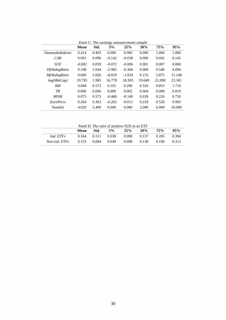
Panel A and B report the summary statistics on quarter short interest ratio (SIR), price, volume, and total net asset value

(TNA) for industry and non-industry ETFs, respectively. The quarter measure is constructed by taking the average of

monthly observations. Panel C reports the summary statistics for firms in our earnings announcement sample.

DummyIndetfown is the dummy variable which equals to 1 if the firm is a member of an industry ETF. CAR is the -1

to +1 cumulative abnormal daily return around the earnings announcement date based on the Fama-French three factor

model. SUE is the standardized earnings surprise computed from a rolling seasonal random walk model. HfAhdngRatio

and MfAhdngRatio are the abnormal holdings from hedge funds and mutual funds, respectively. Both holdings are

standardized by shares outstanding. log(MktCap) is the log transformed market capitalization. BM is the book-to-market

ratio where the book value is measured as the preceding fiscal year, and market value is measured as of the end of that

calendar year. TR is the turnover measured as the average of the daily ratios of volume over shares outstanding from -

40 to -11 of each announcement. MOM is the cumulative raw return over the six-month period ending one month

before the announcement month. EarnPerst is the earnings persistence as of the first-order auto-regressive coefficient

of quarterly earnings over the past four years. NumEst is the number of analysts. Panel D reports the summary statistics

on the ratio of positive SUE in an ETF over our sample period. The positive SUE is defined as the SUE exceeding the

75 percentile of all SUEs in the sample.

Panel A: Industry ETFs

Mean Std. 5% 25% 50% 75% 95%

SIR 0.118 0.211 0.001 0.007 0.026 0.117 0.607

Price 53.842 32.056 18.104 30.167 48.465 68.034 110.976

Volume (in shares) 422847.684 2111222.625 764.333 5382.917 19368.167 75731.833 1963009.083

TNA (in $ millions) 1051.615 2156.886 11.417 91.817 331.200 918.467 5295.167

Panel B: Non-industry ETFs Mean Std. 5% 25% 50% 75% 95%

SIR 0.041 0.118 0.000 0.003 0.008 0.021 0.191

Price 56.290 35.659 15.884 28.185 48.853 75.056 123.672

Volume (in shares) 313927.645 2855881.357 538.017 2304.917 7388.500 32629.167 380683.450

TNA (in $ millions) 2309.432 9704.713 9.467 50.733 179.333 923.600 10578.307

30

Panel C: The earnings announcement sample

Mean Std. 5% 25% 50% 75% 95%

DummyIndetfown 0.414 0.493 0.000 0.000 0.000 1.000 1.000

CAR 0.001 0.096 -0.142 -0.038 0.000 0.041 0.145

SUE -0.002 0.059 -0.072 -0.006 0.001 0.007 0.060

HfAhdngRatio 0.198 2.044 -2.985 -0.304 0.000 0.546 4.094

MfAhdngRatio 0.600 5.826 -8.819 -1.834 0.155 2.875 11.148

log(MktCap) 19.785 1.985 16.778 18.305 19.649 21.098 23.301

BM 0.668 0.573 0.102 0.296 0.526 0.853 1.718

TR 0.006 0.006 0.000 0.002 0.004 0.008 0.019

MOM 0.075 0.373 -0.468 -0.140 0.039 0.226 0.750

EarnPerst 0.264 0.363 -0.263 -0.011 0.218 0.528 0.903

NumEst 4.020 5.400 0.000 0.000 2.000 6.000 16.000

Panel D: The ratio of positive SUE in an ETF

Mean Std. 5% 25% 50% 75% 95%

Ind. ETFs 0.164 0.111 0.038 0.090 0.137 0.205 0.394

Non-ind. ETFs 0.153 0.084 0.049 0.098 0.138 0.190 0.313

31

Table 2: Regress the positive earnings ratio on the lagged short interest at the ETF level

Table 2 reports the result of regressing the positive earnings ratio (𝑃𝑜𝑠𝑆𝑈𝐸𝑖,𝑡) on the lagged short interest ratio

(𝑆𝐼𝑅𝑖,𝑡−1), i.e.,

𝑃𝑜𝑠𝑆𝑈𝐸𝑖,𝑡 = 𝛼𝑖 + 𝛼𝑡 + 𝛽1𝑆𝐼𝑅𝑖,𝑡−1 + 𝑐𝑜𝑛𝑡𝑟𝑜𝑙𝑠 + 𝜖𝑖,𝑡 , (A1)

𝑃𝑜𝑠𝑆𝑈𝐸𝑖,𝑡 = 𝛼𝑖 + 𝛼𝑡 + 𝛽1𝑆𝐼𝑅𝑖,𝑡−1 + 𝛽2𝐷𝑢𝑚𝑚𝑦𝐼𝑛𝑑𝑒𝑡𝑓 × 𝑆𝐼𝑅𝑖,𝑡−1 + 𝑐𝑜𝑛𝑡𝑟𝑜𝑙𝑠 + 𝜖𝑖,𝑡 . (A2)

We run the first regression model on industry and non-industry ETFs, respectively. And we use the second

regression model to estimate the difference in the predicting power of the short interest ratio to the positive

earnings ratio between industry and non-industry ETFs. The difference is captured by 𝛽2 (the coefficient on

𝐷𝑢𝑚𝑚𝑦𝐼𝑛𝑑𝑒𝑡𝑓 × 𝑆𝐼𝑅𝑖,𝑡−1). In our controls, we include log total net asset value, and the year, quarter, and ETF

fixed effect. All standard errors are clustered by ETFs and quarters. Panel A reports the result on full sample, and

Panel B reports the result on full sample excluding year 2007 and 2008. *** is significant at 1%, ** is significant

at 5%, and * is significant at 10%. t-statistic is reported in the parenthesis.

Panel A: Regression result on the full sample

Dependent variable: PosSUE_(i,t) Ind. ETFs Non-ind. ETFs All

SIR_(i,t-1) 0.0324* -0.0235* -0.0253*

(1.6687) (-1.6823) (-1.7972)

DummyIndetf x SIR_(i,t-1) - - 0.0581**

- - (2.481)

log(TNA) 0.0067** 0.0024** 0.0037***

(2.416) (2.2304) (3.0643)

Year F.E. Y Y Y

Quarter F.E. Y Y Y

ETF F.E. Y Y Y

Num.Obs. 4079 9413 13492

R-squared 0.4868 0.6592 0.5855

Panel B: Regression result on the full sample excluding 2007 and 2008

Dependent variable: PosSUE_(i,t) Ind. ETFs Non-ind. ETFs All

SIR_(i,t-1) 0.0436* -0.0124 -0.0174

(1.8814) (-1.0757) (-1.4781)

DummyIndetf x SIR_(i,t-1) - - 0.0625**

- - (2.3364)

log(TNA) 0.0099*** 0.0043*** 0.0058***

(2.7909) (3.2452) (3.8403)

Year F.E. Y Y Y

Quarter F.E. Y Y Y

ETF F.E. Y Y Y

Num.Obs. 3580 8244 11824

R-squared 0.5003 0.6817 0.6054

32

Table 3: The regression result on the market reaction to the earnings surprise

Table 3 reports the regression result on the following model,

𝐶𝐴𝑅𝑖,𝑡 = 𝛼𝑖 + 𝛼𝑡 + 𝜃1𝑆𝑈𝐸𝑖,𝑡 + 𝜃2𝐷𝑢𝑚𝑚𝑦𝐼𝑛𝑑𝑒𝑡𝑓𝑜𝑤𝑛 + 𝜃3𝐷𝑢𝑚𝑚𝑦𝐼𝑛𝑑𝑒𝑡𝑓𝑜𝑤𝑛 × 𝑆𝑈𝐸𝑖,𝑡


(A3)

𝐶𝐴𝑅𝑖,𝑡 is the -1 to +1 cumulative abnormal daily return around the earnings announcement date based on the

Fama-French three factor model. 𝑆𝑈𝐸𝑖,𝑡 is the standardized earnings surprise computed from a rolling seasonal

random walk model. 𝐷𝑢𝑚𝑚𝑦𝐼𝑛𝑑𝑒𝑡𝑓𝑜𝑤𝑛 is a dummy variable, which equals to 1 if the firm is a constituent of

an industry ETF. 𝐷𝑢𝑚𝑚𝑦𝐼𝑛𝑑𝑒𝑡𝑓𝑜𝑤𝑛 × 𝑆𝑈𝐸𝑖,𝑡 is the interaction term. In our control variables, we include the

market capitalization, the book-to-market ratio, the turnover, the momentum factor, the earnings persistence, and

the number of analysts. In addition, we also control for the industry, month, and year fixed effect. All standard

errors are clustered by firms and announcement dates. We run the above regression model on the full sample of

our earnings announcements ranging from 1995 to 2016, except 2007 and 2008. Furthermore, we split our

earnings announcements sample into the “Negative SUE” and “Positive SUE” group based on the earnings

surprise, 𝑆𝑈𝐸𝑖,𝑡. The “Negative SUE” group consists of the bottom 25% 𝑆𝑈𝐸𝑖,𝑡 in our sample, while the “Positive

SUE” group consists of the top 25% 𝑆𝑈𝐸𝑖,𝑡 in our sample. *** is significant at 1%, ** is significant at 5%, and *

is significant at 10%. t-statistic is reported in the parenthesis.

Dependent variable: CAR_(i,t) All Negative SUE Positive SUE

SUE_(i,t) 0.2002*** 0.0944*** 0.0043

(30.8998) (9.6612) (0.3632)

DummyIndetfown 0.007*** 0.0045*** 0.0153***

(9.6669) (3.0769) (9.765)

DummyIndetfown x SUE_(i,t) -0.0551*** -0.014 -0.0464**

(-5.0421) (-0.8049) (-2.4792)

log(MktCap) -0.0014*** 0.0011*** -0.0072***

(-7.3373) (2.9473) (-16.2583)

BM 0.0032*** 0.0036*** 0.0039***

(7.3859) (4.8421) (4.9137)

TR -0.566*** -0.5242*** -0.8457***

(-10.0016) (-5.4694) (-8.2553)

MOM -0.0012 -0.0071*** -0.0021

(-1.3935) (-4.9633) (-1.5745)

EarnPerst 0.0 -0.0016 0.0018

(0.0429) (-1.3259) (1.3534)

NumEst 0.0004*** 0.0007*** 0.0007***

(7.5835) (5.7893) (6.0641)

Industry F.E. Y Y Y

Month F.E. Y Y Y

Year F.E. Y Y Y

Num.Obs. 291599 72715 72922

R-squared 0.0163 0.0116 0.0155

33

Table 4: Hedge funds abnormal holdings and the earnings surprise






(A4)

𝐻𝑓𝐴ℎ𝑑𝑛𝑔𝑅𝑎𝑡𝑖𝑜𝑖,𝑡 is the abnormal holdings by hedge funds standardized by total shares outstanding. The

abnormal holdings are estimated as the difference between the current quarter holdings and the moving average

of holdings in past four quarters. 𝑆𝑈𝐸𝑖,𝑡 is the standardized earnings surprise computed from a rolling seasonal











Dependent variable: HfAhdngRatio_(i,t) All Negative SUE Positive SUE

SUE_(i,t) 0.1345 0.0428 0.2352

(1.5702) (0.3039) (1.3629)

DummyIndetfown -0.0363* 0.0164 -0.1041***

(-1.9484) (0.4293) (-2.8134)

DummyIndetfown x SUE_(i,t) 0.0735 -0.0181 0.931**

(0.3437) (-0.0554) (2.1608)

log(MktCap) -0.0122*** 0.0108 0.0226***

(-3.1918) (1.3304) (2.9731)

BM 0.0197* -0.0169 -0.007

(1.8528) (-0.9672) (-0.4304)

TR 32.3415*** 23.336*** 31.3782***

(23.6757) (9.7707) (13.2446)

MOM 0.034* 0.1052*** 0.0972***

(1.9494) (3.5782) (4.0837)

EarnPerst -0.0672*** 0.0074 -0.0444

(-4.7204) (0.2544) (-1.5082)

NumEst -0.007*** -0.0035 -0.0124***

(-5.2105) (-1.1806) (-4.0509)

Industry F.E. Y Y Y

Month F.E. Y Y Y

Year F.E. Y Y Y

Num.Obs. 291620 72722 72932

R-squared 0.035 0.0397 0.0342

34

Table 5: Mutual funds abnormal holdings and the earnings surprise


𝑀𝑓𝐴ℎ𝑑𝑛𝑔𝑅𝑎𝑡𝑖𝑜𝑖,𝑡 ,

= 𝛼𝑖 + 𝛼𝑡 + 𝜃1𝑀𝑆𝑈𝐸𝑖,𝑡 + 𝜃2

𝑀𝐷𝑢𝑚𝑚𝑦𝐼𝑛𝑑𝑒𝑡𝑓𝑜𝑤𝑛

+ 𝜃3𝑀𝐷𝑢𝑚𝑚𝑦𝐼𝑛𝑑𝑒𝑡𝑓𝑜𝑤𝑛 × 𝑆𝑈𝐸𝑖,𝑡 + 𝑐𝑜𝑛𝑡𝑟𝑜𝑙𝑠 + 𝜖𝑖,𝑡 .

(A5)

𝑀𝑓𝐴ℎ𝑑𝑛𝑔𝑅𝑎𝑡𝑖𝑜𝑖,𝑡 is the abnormal holdings by mutual funds standardized by total shares outstanding. The

abnormal holdings are estimated as the difference between the current quarter holdings and the moving average

of holdings in past four quarters. 𝑆𝑈𝐸𝑖,𝑡 is the standardized earnings surprise computed from a rolling seasonal











Dependent variable: MfAhdngRatio_(i,t) All Negative SUE Positive SUE

SUE_(i,t) 2.5139*** 4.0446*** -4.2241***

(10.6551) (10.0637) (-10.0624)

DummyIndetfown -0.9834*** -0.5686*** -1.1736***

(-14.9465) (-5.2105) (-11.6335)

DummyIndetfown x SUE_(i,t) -0.6845 0.6863 0.8297

(-1.1713) (0.7723) (0.815)

log(MktCap) 0.3333*** 0.3589*** 0.4869***

(19.7558) (13.521) (19.4775)

BM -0.5808*** -0.3701*** -0.381***

(-16.2149) (-7.523) (-8.6381)

TR 71.5907*** -15.8043** 82.3471***

(16.9328) (-2.442) (12.9173)

MOM 2.4397*** 2.38*** 1.5836***

(34.256) (25.9914) (20.9999)

EarnPerst 0.1002** -0.0479 0.1877**

(2.1033) (-0.5969) (2.2023)

NumEst -0.0776*** -0.0396*** -0.0844***

(-16.9889) (-4.6167) (-9.7255)

Industry F.E. Y Y Y

Month F.E. Y Y Y

Year F.E. Y Y Y

Num.Obs. 291620 72722 72932

R-squared 0.0896 0.0694 0.0898

35

Table 6: Fama-MacBeth regression of returns on short interest ratios

Table 6 reports the time-series averages of slope coefficients from Fama and MacBeth (1973) cross-sectional

regressions on returns, 𝑅𝑒𝑡𝑡+1, and changes in the short interest ratio, 𝛥𝑆𝐼𝑅𝑡 , for industry ETFs and their member

firms, respectively. t-statistic reported in the parenthesis is calculated using the average slope coefficient divided

by its time-series standard error adjusted by Newey-West with one lag. For each industry ETF, we average the

member firms’ characteristics and use the average as a control in our regression. We also repeat the Fama-

MacBeth regression on industry ETFs’ member firms and report in the last two columns. For the firm level

regression, the control variable corresponds to each firm’s own characteristics. The sample period of our analysis

is reported in the last row of the table. *** is significant at 1%, ** is significant at 5%, and * is significant at 10%.

Dependent variable: Ret_(t+1) Industry ETFs Member firms

ΔSIR_t 0.019** 0.024*** -0.064** -0.080***

(2.27) (2.65) (-2.32) (-2.83)

Ret from t-12 to t-1 - -0.007 - 0.000

(-0.59) (-0.15)

Ret in month t - 0.003 - -0.014**

(0.09) (-2.13)

BM - -0.001 - 0.002**

(-0.09) (2.12)

Operating profit - 0.001 - 0.000

(0.18) (0.67)

Market capitalization - 0.000 - 0.000

(-0.91) (-1.56)

Asset growth - 0.004 - -0.002

(0.25) (-1.45)

Investment growth - 0.005 - 0.000

(1.32) (-1.36)

Gross profitability - -0.002 - 0.004*

(-0.18) (1.70)

Net stock issuance - -0.009 - 0.000

(-0.39) (0.09)

Accruals - 0.000 - -0.002**

(0.00) (-2.08)

Net operating assets - -0.007 - -0.002

(-0.91) (-0.83)

Intercept 0.013*** 0.010*** 0.009** 0.007*

(3.55) (3.25) (2.46) (1.71)

Sample period 2005.01 - 2006.12,

2009.01 - 2016.11

1999.03 - 2016.11

36

Table 7: Long-short portfolio sorts on ΔSIR

Table 7 reports the average monthly excess returns, CAPM alpha, Fama and French 3-factor alpha, and Fama-

French-Carhart 4-factor alpha for each of the 10 decile portfolios and the High-Low portfolio based on 𝛥𝑆𝐼𝑅. At

the end of each month, all industry ETFs or member firms are sorted into deciles based on 𝛥𝑆𝐼𝑅 in that month.

Then, we track the equal-weighted portfolio returns over the next month. Panel A reports results for industry

ETFs. Holding periods in Panel A is from January 2005 to December 2016, excluding sample in year 2007 and

2008. Panel B reports results for member firms. Member firms with prices below $5 a share or are in the bottom

NYSE size decile are excluded from the sample. Holding period in Panel B is from April 1999 to December 2016.

Standard errors are Newey-West adjusted with one lag.

Panel A: Industry ETFs

Excess returns CAPM alpha 3-factor alpha 4-factor alpha

Decile coef. t-stat. coef. t-stat. coef. t-stat. coef. t-stat.

1 (low) 1.16 2.79 -0.27 -2.29 -0.23 -2.35 -0.20 -2.12

2 1.25 3.06 -0.15 -1.44 -0.12 -1.22 -0.09 -0.91

3 1.37 3.69 -0.17 -1.56 -0.14 -1.33 -0.13 -1.23

4 1.45 4.01 -0.01 -0.08 0.04 0.36 0.04 0.36

5 1.36 3.82 0.07 0.69 0.12 1.22 0.13 1.35

6 1.42 3.79 -0.11 -0.67 -0.04 -0.30 -0.05 -0.33

7 1.36 3.63 0.01 0.13 0.05 0.48 0.06 0.57

8 1.15 2.99 -0.06 -0.55 -0.03 -0.27 -0.01 -0.09

9 1.46 3.65 -0.14 -1.15 -0.10 -0.85 -0.10 -0.83

10 (high) 1.53 3.77 0.02 0.16 0.05 0.44 0.08 0.65

10-1 0.28 2.00 0.29 2.00 0.28 1.97 0.28 1.98

Panel B: Member firms

Excess returns CAPM alpha 3-factor alpha 4-factor alpha

Decile coef. t-stat. coef. t-stat. coef. t-stat. coef. t-stat.

1 (low) 0.81 1.93 0.32 1.55 0.01 0.09 0.05 0.32

2 0.94 2.47 0.49 2.67 0.22 1.67 0.25 1.92

3 0.90 2.53 0.49 2.74 0.24 1.80 0.26 1.93

4 0.98 2.85 0.58 3.32 0.33 2.72 0.34 2.77

5 0.90 2.60 0.52 3.03 0.28 2.29 0.29 2.39

6 1.02 3.04 0.64 3.65 0.37 3.18 0.38 3.24

7 0.94 2.63 0.54 3.06 0.27 2.38 0.29 2.53

8 0.87 2.35 0.44 2.45 0.21 1.52 0.23 1.65

9 0.62 1.59 0.18 0.93 -0.10 -0.71 -0.06 -0.45

10 (high) 0.48 1.08 -0.04 -0.19 -0.35 -2.20 -0.30 -1.95

10-1 -0.33 -3.13 -0.36 -3.37 -0.36 -3.31 -0.35 -3.10

37

Table 8: Hedge fund abnormal holdings and lagged short interest

Table 8 reports the regression result on hedge fund abnormal holdings of industry ETF members and short interest

of the industry ETF.

𝐻𝑓𝐴ℎ𝑑𝑛𝑔𝑅𝑎𝑡𝑖𝑜𝑖,𝑗,𝑡

= 𝛼𝑖 + 𝛼𝑡 + 𝛽1𝑆𝐼𝑅𝑗,𝑡−1 + 𝛽2𝐷𝑢𝑚𝑚𝑦𝑃𝑜𝑠𝑆𝑈𝐸𝑖,𝑡 × 𝑆𝐼𝑅𝑗,𝑡−1 + 𝑐𝑜𝑛𝑡𝑟𝑜𝑙𝑠

+ 𝜖𝑖,𝑡 .

(A6)

𝐻𝑓𝐴ℎ𝑑𝑛𝑔𝑅𝑎𝑡𝑖𝑜𝑖,𝑗,𝑡 is the abnormal holdings by hedge funds (standardized by total shares outstanding) on firm 𝑖

preceding the earnings announcement date 𝑡. Firm 𝑖 is a member of industry ETF 𝑗. 𝑆𝐼𝑅𝑗,𝑡−1 is the lagged short

interest of ETF 𝑗. 𝐷𝑢𝑚𝑚𝑦𝑃𝑜𝑠𝑆𝑈𝐸𝑖,𝑡 is a dummy variable, which equals to 1 if firm 𝑖 has a positive earnings

surprise at 𝑡. We include the market capitalization of firm 𝑖 as our control variable. We also include the year,

quarter, industry, and ETF fixed effect. All standard errors are clustered by ETFs and quarters. We run the above

regression model on the full sample of our earnings announcements ranging from 1995 to 2016, except 2007 and

2008.

Dependent variable: HfAhdngRatio_(i,j,t) Coef.

SIR_(j,t-1) 0.1048

(0.9544)

DummyPosSUE_(i,t) x SIR_(j,t-1) 0.282**

(2.0229)

log(MktCap) -0.0548***

(-8.6449)

Industry F.E. Y

Year F.E. Y

Quarter F.E. Y

ETF F.E. Y

Num.Obs. 343613

R-squared 0.0167

38

Table 9: The regression result on the market reaction to the earnings surprise

Table 9 reports the regression result with firms sorting on the industry risk exposure (the average adjusted 𝑅2

when regressing stock returns on industry ETF returns). Regression models are,



(A7)





(A8)


Fama-French three factor model. 𝐻𝑓𝐴ℎ𝑑𝑛𝑔𝑅𝑎𝑡𝑖𝑜𝑖,𝑡 is the abnormal holdings by hedge funds standardized by

total shares outstanding. 𝑆𝑈𝐸𝑖,𝑡 is the standardized earnings surprise computed from a rolling seasonal random

walk model. 𝐷𝑢𝑚𝑚𝑦𝐼𝑛𝑑𝑒𝑡𝑓𝑜𝑤𝑛 is a dummy variable, which equals to 1 if the firm is a constituent of an industry

ETF. 𝐷𝑢𝑚𝑚𝑦𝐼𝑛𝑑𝑒𝑡𝑓𝑜𝑤𝑛 × 𝑆𝑈𝐸𝑖,𝑡 is the interaction term. In our control variables, we include the market

capitalization, the book-to-market ratio, the turnover, the momentum factor, the earnings persistence, and the

number of analysts. In addition, we also control for the industry, month, and year fixed effect. All standard errors

are clustered by firms and announcement dates. We run the above regression model on the full sample of our

earnings announcements ranging from 1995 to 2016, except 2007 and 2008. Furthermore, we split our earnings

announcements sample into the “Negative SUE” and “Positive SUE” group based on the earnings surprise, 𝑆𝑈𝐸𝑖,𝑡.

The “Negative SUE” group consists of the bottom 25% 𝑆𝑈𝐸𝑖,𝑡 in our sample, while the “Positive SUE” group

consists of the top 25% 𝑆𝑈𝐸𝑖,𝑡 in our sample. *** is significant at 1%, ** is significant at 5%, and * is significant

at 10%. t-statistic is reported in the parenthesis.

Panel A: Regression result on the top and bottom 15% firms sorting on the industry risk exposure

CA

R_(i

,t)

All Negative

SUE

Positive

SUE

HfA

hd

ngR

ati

o_

(i,t

)

All Negative

SUE

Positive

SUE

SUE_(i,t) 0.1488*** 0.0695** 0.0082 0.5135 0.4047 0.8272

(6.7297) (2.1449) (0.2033) (1.2521) (0.6163) (1.0709)

DummyIndetfown 0.0039*** 0.0059* 0.0049 -0.0287 -0.0457 -0.1208

(2.7318) (1.8934) (1.3376) (-0.6538) (-0.5486) (-1.3887)

DummyIndetfown x SUE_(i,t) -0.002 0.0691* -0.0174 -0.4291 -0.0999 0.2364

(-0.0751) (1.6913) (-0.3805) (-0.7416) (-0.1218) (0.2184)

Control and F.E. Y Y Y Y Y Y

Num.Obs. 53111 13250 13269 53113 13251 13270

R-squared 0.0118 0.0169 0.0078 0.0461 0.064 0.0404

Panel B: Regression result on the remains firms

CA

R_(i

,t)

All Negative

SUE

Positive

SUE

HfA

hd

ngR

ati

o_

(i,t

)

All Negative

SUE

Positive

SUE

SUE_(i,t) 0.2042*** 0.0942*** 0.0015 0.0904 0.0262 0.2201

(30.2763) (9.2223) (0.1192) (1.0549) (0.1832) (1.2509)

DummyIndetfown 0.0081*** 0.0057*** 0.0182*** -0.0434** 0.0005 -0.0989**

(9.6302) (3.389) (9.9366) (-2.1076) (0.0121) (-2.3265)

DummyIndetfown x SUE_(i,t) -0.0591*** -0.0206 -0.0496** 0.1868 -0.0369 0.9283*

(-4.8172) (-1.0505) (-2.303) (0.7998) (-0.1) (1.8971)

Control and F.E. Y Y Y Y Y Y

Num.Obs. 238488 59463 59643 238507 59470 59652

R-squared 0.0173 0.0114 0.0165 0.0331 0.0352 0.0325

39

Figure 1: Total net asset value and industry coverage of industry ETFs

Figure 1 shows the time series pattern of total net asset value and industry coverage of industry ETFs from

1998.12.16 (the earliest inception date among our industry ETFs) to 2016.12.31 (the end of our sample period).

The blue line is the total net asset value with measurement on the ETF, and the red line is the industry coverage

with measurement on the right.

40

Figure 2: The histogram of the short interest ratio

Figure 2 shows the histogram of the short interest ratio of industry (top panel) and non-industry ETFs (bottom

panel), respectively. The short interest ratio is sampled quarterly using the average monthly ration in a quarter.

41

Appendix: Additional tests

A1 Including 2007 and 2008 into the analysis

In the main text of the analysis, we exclude the 2007 and 2008 crisis period. This is to

control for the abnormal market movement and regulatory interventions such as the short sale

ban which might bias the overall findings of our analysis. That said, for a robustness check, we

repeat our main analysis including the 2007 and 2008 crisis period in this section.

A1.1 The market reaction and hedge funds abnormal holdings

We include 2007 and 2008 in our sample in analyzing the impact of the industry ETF

membership on the earnings surprise (Table A.1) and the abnormal hedge fund holdings (Table

A.2). Results are largely consistent. The only exception is that the membership also

significantly reduces the market reaction to the negative earnings surprise (Negative SUE).

This appears to be a crisis specific effect, as the sample without 2007 and 2008 shows the

membership has an insignificant impact on the negative earnings surprise.

[Insert Table A.1 here]


A1.2 The return and the short interest

In Table A.3, we report the Fama-MacBeth result on short interest’s return predictability

including the 2007 and 2008. Moreover, we extend our return sample of the industry ETF back

to 2001. Due to data availability, we drop some controls used in the regression in the main text.

We find that the change in the short interest ratio (𝛥𝑆𝐼𝑅) of an industry ETF positively predicts

its future return. This is consistent with our results in the main text. We are unable to construct

the long-short portfolio with this extended sample, since there are less than 30 industry ETFs

in the early 2000s (see Figure A.1).

42


A2 Robustness check with a less strict industry ETF list

We obtain the list of industry ETFs using the following three steps:

(1). We require that the most considerable industry investment exceeds one-third of the

ETF’s portfolio size. This gives us 217 industry ETFs.

(2). We filter out ETFs whose name contains “value,” “growth,” “Russell,” “dividend,” or

“momentum” to ensure the ETF targets for the industry coverage. After this step, we

are left with 150 ETFs.

(3). We further require that the ETF consists of at least 30 stocks. This yields a final list of

116 industry ETFs.

We repeat our main analysis (on earnings surprise and hedge fund abnormal holdings) with

the industry ETF list generated from step 1 and 2 (not including 3). This gives us a less strict

industry ETF list and a larger sample size. We find results consistent with our previous

findings.



A3 Short interest at the stock level

We report short interest of our sample stocks in Table A.6. We split our sample based on

the industry ETF membership, and then report short interest for stocks in industry ETFs and

not in industry ETFs, respectively.


43

Table A.1: The regression result on the market reaction to the earnings surprise

(including 2007 and 2008)

Table A.1 reports the regression result on the following model,



(A9)








our earnings announcements ranging from 1995 to 2016. Furthermore, we split our earnings announcements

sample into the “Negative SUE” and “Positive SUE” group based on the earnings surprise, 𝑆𝑈𝐸𝑖,𝑡. The “Negative

SUE” group consists of the bottom 25% 𝑆𝑈𝐸𝑖,𝑡 in our sample, while the “Positive SUE” group consists of the top

25% 𝑆𝑈𝐸𝑖,𝑡 in our sample. *** is significant at 1%, ** is significant at 5%, and * is significant at 10%. t-statistic

is reported in the parenthesis.


SUE_(i,t) 0.2029*** 0.1004*** 0.0023

(31.8979) (10.3802) (0.1974)

DummyIndetfown 0.0075*** 0.0044*** 0.0159***

(10.6741) (3.0943) (10.5351)

DummyIndetfown x SUE_(i,t) -0.0598*** -0.034* -0.0476***

(-5.4437) (-1.9563) (-2.6286)

log(MktCap) -0.0013*** 0.0011*** -0.0071***

(-7.1289) (2.8089) (-16.5959)

BM 0.0035*** 0.0043*** 0.0039***

(8.0445) (5.6134) (4.9229)

TR -0.506*** -0.4774*** -0.798***

(-9.3207) (-5.1607) (-8.2472)

MOM -0.0013 -0.0075*** -0.0017

(-1.4812) (-5.3127) (-1.2873)

EarnPerst 0.0002 -0.001 0.0023*

(0.4293) (-0.8273) (1.831)

NumEst 0.0004*** 0.0007*** 0.0007***

(7.7999) (6.4169) (6.0764)

Industry F.E. Y Y Y

Month F.E. Y Y Y

Year F.E. Y Y Y

Num.Obs. 320602 79955 80157

R-squared 0.016 0.0118 0.0147

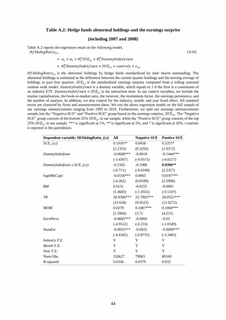
44

Table A.2: Hedge funds abnormal holdings and the earnings surprise

(including 2007 and 2008)

Table A.2 reports the regression result on the following model,





(A10)


abnormal holdings is estimated as the difference between the current quarter holdings and the moving average of

holdings in past four quarters. 𝑆𝑈𝐸𝑖,𝑡 is the standardized earnings surprise computed from a rolling seasonal




the number of analysts. In addition, we also control for the industry, month, and year fixed effect. All standard errors are clustered by firms and announcement dates. We run the above regression model on the full sample of

our earnings announcements ranging from 1995 to 2016. Furthermore, we split our earnings announcements

sample into the “Negative SUE” and “Positive SUE” group based on the earnings surprise, 𝑆𝑈𝐸𝑖,𝑡. The “Negative

SUE” group consists of the bottom 25% 𝑆𝑈𝐸𝑖,𝑡 in our sample, while the “Positive SUE” group consists of the top

25% 𝑆𝑈𝐸𝑖,𝑡 in our sample. *** is significant at 1%, ** is significant at 5%, and * is significant at 10%. t-statistic

is reported in the parenthesis.


SUE_(i,t) 0.1916** 0.0458 0.3357*

(2.2355) (0.3293) (1.9372)

DummyIndetfown -0.0608*** -0.0019 -0.1444***

(-3.4567) (-0.0515) (-4.0217)

DummyIndetfown x SUE_(i,t) -0.1503 -0.1988 0.9396**

(-0.711) (-0.6248) (2.2357)

log(MktCap) -0.0156*** 0.0065 0.0197***

(-4.262) (0.8189) (2.5996)

BM 0.0151 -0.0255 -0.0081

(1.4683) (-1.4555) (-0.5107)

TR 30.9306*** 22.7002*** 28.0551***

(23.628) (9.9523) (12.0272)

MOM 0.0279 0.1087*** 0.1004***

(1.5964) (3.7) (4.231)

EarnPerst -0.0685*** -0.0066 -0.03

(-4.9512) (-0.233) (-1.0349)

NumEst -0.0055*** -0.0025 -0.0099***

(-4.4345) (-0.8735) (-3.3483)

Industry F.E. Y Y Y

Month F.E. Y Y Y

Year F.E. Y Y Y

Num.Obs. 320627 79963 80169

R-squared 0.0336 0.0379 0.032

45

Table A.3: Fama-MacBeth regression of returns on short interest ratios

Table A.3 reports the time-series averages of slope coefficients from Fama and MacBeth (1973) cross-sectional

regressions on returns, 𝑅𝑒𝑡𝑡+1, and changes in the short interest ratio, 𝛥𝑆𝐼𝑅𝑡 , for industry ETFs and their member

firms, respectively. t-statistic reported in the parenthesis is calculated using the average slope coefficient divided

by its time-series standard error adjusted by Newey-West with one lag. For each industry ETF, we average the

member firms’ characteristics, and use the average as a control in our regression. We also repeat the Fama-

MacBeth regression on industry ETFs’ member firms, and report in the last columns. For the firm level regression,

the control variable corresponds to each firm’s own characteristics. The sample period of our analysis is reported

in the last row of the table. *** is significant at 1%, ** is significant at 5%, and * is significant at 10%.

Dependent variable: Ret_(t+1) Industry ETFs Member firms

ΔSIR_t 0.016** -0.059**

(2.48) (-2.22)

Ret from t-12 to t-1 0.001 -0.000

(0.12) (-0.05)

Ret in month t 0.013 -0.011

(0.46) (-1.57)

BM 0.000 0.001*

(-0.08) (1.65)

Market capitalization 0.000 -0.000

(-0.44) (-1.60)

Intercept 0.005 0.007**

(1.64) (2.00)

Sample period 2001.06 - 2016.11 1998.04-2016.11

46

Table A.4: The regression result on the market reaction to the earnings surprise

(less strict ETF list)

Table A.4 reports the regression result on,



(A11)














SUE_(i,t) 0.2004*** 0.0948*** 0.0037

(30.856) (9.6808) (0.3097)

DummyIndetfown 0.0071*** 0.0046*** 0.0153***

(9.6571) (3.1449) (9.6794)

DummyIndetfown x SUE_(i,t) -0.0553*** -0.0152 -0.0442**

(-5.0768) (-0.8806) (-2.364)

log(MktCap) -0.0014*** 0.0011*** -0.0072***

(-7.357) (2.8976) (-16.2355)

BM 0.0032*** 0.0036*** 0.0039***

(7.378) (4.8352) (4.8979)

TR -0.5672*** -0.5273*** -0.8462***

(-10.0175) (-5.4954) (-8.2668)

MOM -0.0012 -0.0071*** -0.0021

(-1.3866) (-4.9477) (-1.5724)

EarnPerst 0.0 -0.0016 0.0017

(0.0336) (-1.3265) (1.3427)

NumEst 0.0004*** 0.0007*** 0.0007***

(7.5917) (5.7914) (6.071)

Industry F.E. Y Y Y

Month F.E. Y Y Y

Year F.E. Y Y Y

Num.Obs. 291599 72715 72922

R-squared 0.0163 0.0116 0.0155

47

Table A.5: Hedge funds abnormal holdings and the earnings surprise

(less strict ETF list)

Table A.5 reports the regression result on,





(A12)


abnormal holdings is estimated as the difference between the current quarter holdings and the moving average of

holdings in past four quarters. 𝑆𝑈𝐸𝑖,𝑡 is the standardized earnings surprise computed from a rolling seasonal




the number of analysts. In addition, we also control for the industry, month, and year fixed effect. All standard errors are clustered by firms and announcement dates. We run the above regression model on the full sample of







SUE_(i,t) 0.1134 -0.001 0.2257

(1.3305) (-0.0072) (1.3097)

DummyIndetfown -0.0358* 0.0213 -0.1028***

(-1.9379) (0.5563) (-2.7867)

DummyIndetfown x SUE_(i,t) 0.1464 0.1243 0.96**

(0.6789) (0.3755) (2.2369)

log(MktCap) -0.0123*** 0.011 0.0223***

(-3.2324) (1.352) (2.9388)

BM 0.0197* -0.0169 -0.007

(1.8526) (-0.9681) (-0.4325)

TR 32.3505*** 23.4393*** 31.3446***

(23.7129) (9.8371) (13.2313)

MOM 0.034* 0.1048*** 0.0973***

(1.9494) (3.5668) (4.0882)

EarnPerst -0.0671*** 0.0073 -0.0443

(-4.7184) (0.2506) (-1.5041)

NumEst -0.007*** -0.0035 -0.0124***

(-5.2056) (-1.1868) (-4.0483)

Industry F.E. Y Y Y

Month F.E. Y Y Y

Year F.E. Y Y Y

Num.Obs. 291620 72722 72932

R-squared 0.035 0.0397 0.0342

48

Table A.6: Stock level short interest

Table A.6 reports the summary statistics of stock level short interest for our sample stocks. We break our sample

stocks into two groups: 1). Stocks with industry ETF membership; 2). Stocks without industry ETF membership.

Mean Std. 5% 25% 50% 75% 95%

In industry ETF 0.052 0.058 0.003 0.015 0.032 0.067 0.166

Out industry ETF 0.039 0.053 0.0 0.005 0.02 0.05 0.142

49

Figure A.1: The number of industry ETFs in our sample over time

Figure A.1 shows the number of industry ETFs (yearly) in our sample.

Documents

Innovation and Informed Trading: Evidence from Industry ETFsshort-sale constraints in the underlying stock increase violations of put-call parity, suggesting that the difficulty in