Injection Locking Of Semiconductor Mode-locked Lasers For

University of Central Florida University of Central Florida

STARS STARS

Electronic Theses and Dissertations, 2004-2019

2013

Injection Locking Of Semiconductor Mode-locked Lasers For Injection Locking Of Semiconductor Mode-locked Lasers For

Long-term Stability Of Widely Tunable Frequency Combs Long-term Stability Of Widely Tunable Frequency Combs

Charles Williams University of Central Florida

Part of the Electromagnetics and Photonics Commons, and the Optics Commons

Find similar works at: https://stars.library.ucf.edu/etd

University of Central Florida Libraries http://library.ucf.edu

This Doctoral Dissertation (Open Access) is brought to you for free and open access by STARS. It has been accepted

for inclusion in Electronic Theses and Dissertations, 2004-2019 by an authorized administrator of STARS. For more

information, please contact [email protected].

STARS Citation STARS Citation Williams, Charles, "Injection Locking Of Semiconductor Mode-locked Lasers For Long-term Stability Of Widely Tunable Frequency Combs" (2013). Electronic Theses and Dissertations, 2004-2019. 2594. https://stars.library.ucf.edu/etd/2594

https://stars.library.ucf.edu/



https://stars.library.ucf.edu/etd

http://network.bepress.com/hgg/discipline/271?utm_source=stars.library.ucf.edu%2Fetd%2F2594&utm_medium=PDF&utm_campaign=PDFCoverPages

http://network.bepress.com/hgg/discipline/204?utm_source=stars.library.ucf.edu%2Fetd%2F2594&utm_medium=PDF&utm_campaign=PDFCoverPages

https://stars.library.ucf.edu/etd

http://library.ucf.edu/

mailto:[email protected]

https://stars.library.ucf.edu/etd/2594?utm_source=stars.library.ucf.edu%2Fetd%2F2594&utm_medium=PDF&utm_campaign=PDFCoverPages



INJECTION LOCKING OF SEMICONDUCTOR MODE-LOCKED LASERS FOR LONG-TERM STABILITY OF WIDELY TUNABLE FREQUENCY COMBS

by

CHARLES G. WILLIAMS B.S. University of Missouri – Rolla, 2006 M.S. University of Central Florida, 2008

A dissertation submitted in partial fulfillment of the requirements for the degree of Doctor of Philosophy in the College of Optics and Photonics

at the University of Central Florida Orlando, Florida

Spring Term 2013

Major Professor: Peter J. Delfyett

ii

© 2013 Charles G Williams

iii

ABSTRACT

Harmonically mode-locked semiconductor lasers with external ring cavities offer

high repetition rate pulse trains while maintaining low optical linewidth via long cavity

storage times. Single frequency injection locking generates widely-spaced and tunable

frequency combs from these harmonically mode-locked lasers, while stabilizing the

optical frequencies. The output is stabilized long-term with the help of a feedback loop

utilizing either a novel technique based on Pound-Drever-Hall stabilization or by

polarization spectroscopy. Error signals of both techniques are simulated and compared

to experimentally obtained signals. Frequency combs spaced by 2.5 GHz and ~10 GHz

are generated, with demonstrated optical sidemode suppression of unwanted modes of

36 dB, as well as RF supermode noise suppression of 14 dB for longer than 1 hour. In

addition to the injection locking of actively harmonically mode-locked lasers, the

injection locking technique for regeneratively mode-locked lasers, or Coupled Opto-

Electronic Oscillators (COEOs), is also demonstrated and characterized extensively.

iv

For my wife, Allison, who locks me away in rooms to force help me to write, and brings

me food and encouragement all the while.

And for my mother, Joyce, who did the same for many years of my life to get me to this

point, when the writing had more to do with the Titanic than Injection Locked Lasers.

v

ACKNOWLEDGMENTS

I would first like to acknowledge Prof. Peter Delfyett for his teaching and

guidance throughout my dissertation research, as well as my CREOL professors and

committee members for the same: Professors Patrick LiKamWa, Eric Van Stryland, and

David Hagan, and Dr. Richard DeSalvo. I owe a great deal of my early understanding of

lasers and scientific training to my former labmate, Dr. Franklyn Quinlan.

In addition, many members of the Ultrafast Photonics Group, past and present,

have helped immensely in thinking and talking through the concepts herein. Those in

particular whose discussions and vigorous debates have stood out in my mind are: Dr.

Sangyoun Gee, Dr. Dimitrios Mandridis, Dr. Josue Davila-Rodriguez, Dr. Nazanin

Hoghooghi, Marcus Bagnell, Tony Klee, Kristina Bagnell, Dr. Sarper Ozharar, Dr.

Ibrahim Ozdur, Dr. Ji-Myung Kim, Abhijeet Ardey, and Edris Sarailou.

Separately, I would like to acknowledge the work of all past UP members, whose

work I was privileged to build upon, and those I have been in the group with for sharing

your research and allowing me to gain knowledge and experience far beyond what I

could gather on my own.

Lastly, many friends in CREOL and out have helped immensely in scientific

discussions, paper editing, and moral support: Dr. Matthew Weidman, Mark Ramme,

Dr. John Broky, Matthew Weed, James Williams Jr., Dr. Robert Bernath, Dr. Casey

Boutwell, Kyle Douglass and countless others in ways large and small.

vi

TABLE OF CONTENTS

LIST OF FIGURES ........................................................................................................................................................ VIII

LIST OF ABBREVIATIONS ............................................................................................................................................. XIII

CHAPTER 1: INTRODUCTION .......................................................................................................................................... 1

1.1 Definitions ........................................................................................................................................................... 2 1.2 Applications ......................................................................................................................................................... 3

1.2.1 Optical Time Domain Multiplexing .............................................................................................................. 3 1.2.2 Optical Arbitrary Waveform Generation ..................................................................................................... 4 1.2.3 Coherent Communication ............................................................................................................................ 5 1.2.4 RF Photonics and Optical Clocks .................................................................................................................. 6 1.2.5 Multiheterodyne Spectroscopy ................................................................................................................... 7 1.2.6 Photonic Analog-to-Digital Conversion ........................................................................................................ 9

CHAPTER 2: HARMONICALLY MODE-LOCKED LASERS ................................................................................................. 11

2.1 Harmonic Mode-Locking Mechanism................................................................................................................ 11 2.2 Sources of Noise in Harmonically Mode-Locked Lasers .................................................................................... 12

CHAPTER 3: INJECTION LOCKING OF OSCILLATORS ..................................................................................................... 14

3.1 Applications of Injection Locking ....................................................................................................................... 16 3.2 Semiconductor Cavity Dynamics of Injection Locking ....................................................................................... 17

CHAPTER 4: LASER CAVITY STABILIZATION VIA POUND-DREVER-HALL METHOD ....................................................... 22

4.1 Pound-Drever-Hall Cavity Stabilization Overview ............................................................................................. 22 4.2 Modified Pound-Drever-Hall Stabilization Error Signal Simulation ................................................................... 25

4.2.1 Conventional Pound-Drever-Hall Error Signal ............................................................................................ 25 4.2.2 Simulated Cavity Resonances .................................................................................................................... 28 4.2.3 Modified Pound-Drever-Hall Simulations .................................................................................................. 30

CHAPTER 5: CW INJECTION LOCKING OF AN ACTIVELY MODE-LOCKED LASER ........................................................... 38

5.1 Actively Mode-Locked Injection Locked Laser Setup ........................................................................................ 38 5.2 Laser Preparation for Frequency Comb Generation ......................................................................................... 40

5.2.1 Laser Parameters for Effective Injection Locking ....................................................................................... 40 5.2.2 Injection Locking Procedure ....................................................................................................................... 41 5.2.3 Pound-Drever-Hall Stabilization Error Signal Locking Exploration ............................................................. 43

5.3 Actively mode-locked injection locked laser results ......................................................................................... 46

CHAPTER 6: LASER CAVITY STABILIZATION VIA POLARIZATION SPECTROSCOPY ........................................................ 51

6.1 Polarization Spectroscopy: Introduction and Experimental Setup.................................................................... 52 6.1.1 Polarization Spectroscopy Error Signal Locking Exploration ...................................................................... 53

6.2 Polarization Spectroscopy Stabilization Error Signal Simulation ....................................................................... 56 6.2.1 Simulated Cavity Resonances .................................................................................................................... 56

6.3 Stabilization via Polarization Spectroscopy: Results and Conclusion ................................................................ 59

vii

CHAPTER 7: CW INJECTION LOCKING OF A COUPLED OPTO-ELECTRONIC OSCILLATOR ............................................. 61

7.1 Regenerative Mode-Locking .............................................................................................................................. 62 7.2 Injection Locked COEO Experimental Setup ...................................................................................................... 64 7.3 Injection Locked COEO Results .......................................................................................................................... 66

7.3.1 Optical, RF Spectra and Time Domain Traces ............................................................................................ 66 7.3.2 Amplitude and Phase Noise ....................................................................................................................... 71 7.3.3 Allan Deviation ........................................................................................................................................... 75

7.4 RF Frequency dependence on Injected Optical Frequency of Injection Locked COEO ..................................... 78 7.4.1 Experimental Results ................................................................................................................................. 80 7.4.2 Discussion and Conclusion ......................................................................................................................... 82

CHAPTER 8: CONCLUSION ........................................................................................................................................... 83

APPENDIX A: ALLAN DEVIATION MEASUREMENT ...................................................................................................... 84

Equation and its Explanation ................................................................................................................................... 88 Experimental Measurement ................................................................................................................................... 89 Simulation ............................................................................................................................................................... 91 Examples and Explanations ..................................................................................................................................... 94

APPENDIX B: LIST OF PUBLICATIONS AND CONFERENCES ....................................................................................... 104

Primary Author ...................................................................................................................................................... 105 Secondary Author .................................................................................................................................................. 106

APPENDIX C: MATLAB CODE USED FOR SIMULATIONS ............................................................................................. 109

Pound Drever Hall and Polarization Spectroscopy Error Signal ............................................................................ 110 Allan Deviation Simulation .................................................................................................................................... 116

REFERENCES ............................................................................................................................................................... 118

viii

LIST OF FIGURES

Figure 1.1 Schematic of Optical Time Domain Multiplexing as a utilization of mode-locked laser pulse trains. Pulses are directed to different modulating signals via an active optical switching mechanism. Each user then sees a lower repetition rate pulse train on which to impart a signal. Original pulse train is reconstituted and transmitted to another switch, separated again, and sent to corresponding receivers. 4 Figure 1.2 Schematic of Optical Arbitrary Waveform Generation (OAWG). Individual frequency components of a frequency comb are isolated via wavelength division multiplexing (WDM), affected individually using phase and amplitude modulation (PM and AM, respectively). When remultiplexed, a repetitive arbitrary optical signal is generated. ............................................................................................ 5 Figure 1.3 Schematic of an optical coherent communication setup. Each optical frequency component of a frequency comb is encoded by a unique user’s signal, resulting in a seemingly arbitrary signal sent to the receiver side, where the individual signals are demultiplexed and received individually. .................... 6 Figure 1.4 Conceptual diagram of photonic enabled RF arbitrary waveform generation. An RF waveform corresponding to the intensity of the arbitrary optical waveform is generated with instantaneous frequency up to that of the photodetector bandwidth. ............................................................................... 7 Figure 1.5 Schematic and concept of multiheterodyne spectroscopy. Two mode-locked lasers with differing repetition rates are combined and photodetected. Comblines from each laser are paired up to produce a spectrum of RF heterodyne beats, preserving the relative frequency and phase between combline pairs. .............................................................................................................................................. 8 Figure 1.6 A generalized picture of photonic enabled analog-to-digital conversion wherein mode-locked laser pulses with ultra-low timing jitter and pulse-to-pulse energy fluctuations are modulated using the signal to be converted. Each pulse samples the waveform at a set interval and its amplitude value can then be independently recorded in digital format. .................................................................................... 10 Figure 2.1 Fundamental (a) versus harmonic (b) mode-locking in the time domain for laser cavities of the same length showing multiple pulses traversing the harmonically mode-locked cavity. Representations of the spectral output in the fundamental (c) and harmonic (d) mode-locking cases showing the presence of optical supermode sets in a HMLL. The Semiconductor Optical Amplifier (SOA) gain media are shown as red triangles and the IMs are shown in the lower part of the cavities, along with the input sine wave to the respective modulators. In this example the HMLL contains three pulses traversing the cavity.................................................................................................................................... 12 Figure 3.1. A slaved cavity resonance and its relevant injection locking properties. The locking range is demonstrated by the vertical cyan lines, as well as the injection lock phase limits of ± π/2, while the regenerative gain curve of the resonance (solid blue lines) is shown versus optical frequency.Within the locking range, the normalized output power is clamped, approximated by a higher order Gaussian (green circles). The normalized transmission of a passive cavity, defined by the real part of the Airy function, is shown in solid green. The phase shift that an injected tone experiences as it moves across the resonance is shown in red and is shown as an arcsin shape extending from π/2 to - π/2 over the locking range. .............................................................................................................................................. 15

ix

Figure 3.2. Semiconductor laser cavity resonances with non-zero alpha parameters, shifting resonance phase downward and broadening the injection locking range. Note the difference in frequency scale between figure a) and figures b) and c). ..................................................................................................... 19 Figure 4.1. Representation of the injection seed frequency and phase modulation sidebands injected into a HMLL. Note that the phase modulation sidebands are not resonant with the optical cavity when the injection seed frequency is within a cavity resonance injection locking range.................................... 24 Figure 4.2. a) Conventional PDH Error Signal derived from a cavity with R = 0.99 and PM frequency of 1.13*FSR. b) Passive FPE cavity normalized transmission (blue) and phase (green), according to the Airy function governing passive cavity behavior. ............................................................................................... 27 Figure 4.3. Cavity amplitude and phase response within injection locking ranges for the center resonance and two nearest neighbor resonances, which PM sidebands interact with while the carrier is near zero detuning. ..................................................................................................................................... 29 Figure 4.4. Comparison of experimentally obtained error signal (blue, PM frequency ~ 15.047*FSR) to simulated error signal (red) with the parameters shown. The multiple cavity amplitude responses are shown in green, while their phase responses are shown in cyan............................................................... 32 Figure 4.5. Comparison of experimentally obtained error signal (blue) to simulated error signal (red), as well as copies of simulated signals shifted by one FSR in the positive detuning direction (pink) and negative detuning direction (black) to illustrate the origin of triangle waveform features between each cavity resonance. ........................................................................................................................................ 34 Figure 4.6. Comparison of realistic locking signal to simulation results. Visual fitting was able to closely approximate either a) the center features including the differential features used for feedback stabilization, or b) the overall shape of the error signal. ............................................................................ 36 Figure 5.1. Laser system schematic of actively mode-locked injection locked laser with long-term feedback. BPF: Optical Bandpass Filter; DBM: RF Double Balanced Mixer; DCF: Dispersion Compensating Fiber; FPS: Fiber Phase Shifter; IC: Injection Coupler; IM: Intensity Modulator; IPM: Injection Power Monitor; IS: Isolator; ISL: Injection Seed Laser; LPF: RF Low Pass Filter; OC: Output Coupler; PC: Polarization Controller; PD: Photodetector; PIC: PI Controller; PM: Phase Modulator; PS: RF Phase Shifter; RFA: Low Noise RF Amplifier; SOA: Semiconductor Optical Amplifier; VOA: Variable Optical Attenuator; VOD: Variable Optical Delay.................................................................................................... 39 Figure 5.2. a) Optical and b) Photodetected RF spectra of a harmonically mode-locked laser with injection from the single frequency injection laser, but not yet injection-locked. .................................... 42 Figure 5.3. Error Signal for laser system stabilization via PDH. The system was temporarily stabilized at the labeled points shown for observation of the locking characteristics, shown in the following figure. . 44 Figure 5.4. a) Optical (0.05 nm resolution) and b) RF (60 MHz span; 6.8 kHz RBW) spectral observations of injection locking at various points along the PDH error signal, shown in the previous figure. Optimal injection locking was found at point ‘G’ (light purple). Other injection points of decent quality (points ‘D’ and ‘I’) occur where PM sidebands are aligned with other cavity resonances and therefore injection lock them. ........................................................................................................................................................... 45 Figure 5.5. Optical spectra of the actively mode-locked laser free running, or without optical injection (black) and injection locked (red). (a) shows the entire mode-locked spectrum, while (b) is a high

x

resolution view of a portion of the spectra. Two tones of the injection selected supermode are visible with a spacing of 2.5 GHz, while 36 dB suppression of the unselected supermodes is shown. ................. 46 Figure 5.6. RF spectra of the laser system in the free running (black) and injection locked (red) case. (a) shows the suppression of RF supermode noise spurs by 14 dB due to optical injection. In (b) the suppression of RF supermode noise spurs for fifteen minutes is shown while the modified PDH feedback loop is in use. .............................................................................................................................................. 48 Figure 5.7. (a) Modified Pound-Drever-Hall error signal of the injection locked actively mode-locked laser cavity with CW injection. The discriminant portion of the error signal used for locking the cavity is highlighted in red. (b) Ideal Pound-Drever-Hall error signal shape for a passive cavity such as an etalon. The discriminant is the sharp vertical line in the center feature of the signal. .......................................... 49 Figure 5.8. Residual phase noise of the laser in free running and injection locked states. In free running operation, an integrated timing jitter from 1Hz to 100 MHz of 427 fs was measured. Optical injection reduced the integrated jitter to 121 fs. ...................................................................................................... 50 Figure 5.9. Pulse-to-pulse energy fluctuation, or amplitude noise of the laser in free running and injection locked states. In free running operation, integrated AM noise from 1Hz to 100 MHz of 0.61% was measured. Optical injection reduced this integrated AM noise to 0.24%. ......................................... 50 Figure 6.1. Schematic of injection locked HMLL with long-term stabilization via polarization spectroscopy. .............................................................................................................................................. 52 Figure 6.2. Error Signal for laser system stabilization via polarization spectroscopy. The system was temporarily stabilized at the labeled points shown for observation of the locking characteristics, shown in the following figure. ................................................................................................................................ 54 Figure 6.3. a) Optical (0.05 nm resolution) and b) RF (60 MHz span; 6.8 kHz RBW) spectral observations of injection locking at various points along the HC error signal, shown in the previous figure. Optimal injection locking was found at point ‘K’ (dark blue), while best error signal locking was found at point ‘E’. .................................................................................................................................................................... 55 Figure 6.4. Amplitude (blue) and phase (green) response of slaved cavity resonance with gain, as well as original HC error signal (red) and signal of the HC technique applied to a semiconductor cavity with gain (teal). ........................................................................................................................................................... 57 Figure 6.5. Experimentally obtained polarization spectroscopy error signal (green) comparison to simulated (blue). ......................................................................................................................................... 58 Figure 6.6. (a) Optical spectra of HMLL not subject to optical injection (black) and injection locked and stabilized via polarization spectroscopy (blue). (b) High resolution optical spectra of HMLL output showing frequency comb generation under optical injection with high OSNR. The latter curve was artificially offset by -10 dB to illustrate the absence of PM sidebands on each combline. ........................ 59 Figure 6.7. Photodetected RF spectra of the injection locked laser stabilized via the two methods. Note the absence of an RF sideband 550 MHz offset from the 10.24 GHz carrier for the HC stabilization method. ....................................................................................................................................................... 60 Figure 7.1 Schematic of a typical Coupled Opto-Electronic Oscillator. The optical cavity is shown in blue, with gain (red triangle) and intensity modulator (left). The electronic part of the opto-electronic cavity is

xi

shown in black, where the output is photodetected (right), filtered (not shown for simplicity), amplified (black triangle) and fed back into the intensity modulator. ....................................................................... 63 Figure 7.2 Injection Locked COEO system schematic. BPF, Bandpass Filter; DBM, Double Balanced Mixer; DCF, Dispersion Compensating Fiber; FPS, Fiber Phase Shifter; IC, Injection Coupler; IM, Intensity Modulator; ISL, Injection Seed Laser; ISO, Isolator; LPF, Lowpass Filter; OC, Output Coupler; PC, Polarization Controller; PD, Photodetector; PIC, Proportional-Integral Controller; PM, Phase Modulator; PS, Phase Shifter; RFA, RF Amplifier; SOA, Semiconductor Optical Amplifier. ........................................... 65 Figure 7.3 (a) Optical spectra of the free-running (black) and injection-locked (red) states. The injection seed frequency is denoted by a black arrow. (b) High resolution optical spectra (100 MHz resolution). The optical modes in free-running operation (black) are too closely spaced (11 MHz) for the instrument to resolve. ................................................................................................................................................... 67 Figure 7.4 (a) RF power spectrum of the photodetected COEO optical output, free-running (black) and injection-locked (red) with fundamental RF tone and one supermode noise spur, suppressed via injection locking. (b) Zoomed view of fundamental RF tones at ~10.24 GHz. ............................................ 69 Figure 7.5 Time domain normalized (a) sampling scope and (b) autocorrelation traces of the COEO output in both free-running (black) and injection-locked (red) cases. ....................................................... 70 Figure 7.6 Power spectral density of the amplitude noise of the injection-locked COEO for various injection powers: black, free-running; red,~9 µW; cyan, 14 µW; orange, 20 µW. Pulse-to-pulse energy fluctuation for each case, integrated from higher to lower offset frequencies. ........................................ 71 Figure 7.7 Supermode noise spur detail of the absolute phase noise power spectral density of the COEO system in the free-running (black) and injection-locked (red) cases. Blue dashed peaks are spurious results of the frequency discriminator measurement. Offset frequency is shown in linear scale to highlight the suppression of supermode noise spurs at higher offsets. Arrows indicate modes used in timing jitter estimation. .............................................................................................................................. 73 Figure 7.8 Allan Deviation measurements of the Injection Locked COEO from the photodetected optical output for both injection locked (red triangle) and free-running (black) states. ....................................... 76 Figure 7.9 (a) Schematic of the injection locked COEO with feedback stabilization. (b) Experimental setup for measurement of optical-to-RF instability transfer. ............................................................................... 79 Figure 7.10 (a) Allan Deviation measurements of the free-running and injection locked COEO, as well as of heterodyne beat signals between the injection seed lasers and an optical frequency reference. (b) Instability transfer from the optical injection frequency to the COEO RF output via sinusoidal modulation of the injection seed frequency. ................................................................................................................. 81 Figure A.1 Simulated instantaneous frequency values of a non-stable signal at a starting frequency of 10 GHz. ............................................................................................................................................................. 87 Figure A.2 Typical Allan Deviation plot showing calculated fractional deviation values for increasing measurement times. ................................................................................................................................... 88 Figure A.3 a) Oscillating signal of interest in blue with zero crossings shown by black dots. Boxes shown represent average frequency measurement times of b) 100 ns, c) 1 μs, d) 10 μs, and e) 100 μs. ............ 90 Figure A.4 Instantaneous frequency values (blue) and averages (black) over four instantaneous time increments. ................................................................................................................................................. 92

xii

Figure A.5 Instantaneous frequency values (blue) and averages (light blue) over 16 instantaneous time increments. ................................................................................................................................................. 92 Figure A.6 Instantaneous frequency values (blue) and averages (green) over 64 instantaneous time increments. ................................................................................................................................................. 93 Figure A.7 Instantaneous frequency values (blue) and averages (blue straight lines) over 256 instantaneous time increments. ................................................................................................................. 93 Figure A.8 Instantaneous frequency values (top, blue) and averages over several instantaneous time increments. ................................................................................................................................................. 94 Figure A.9 a) Instantaneous frequency values starting at 10 GHz and calculated with equal parts white noise and random walk. b) ADEV curve of the frequency values. c) Modified STDEV curve (blue) and difference between ADEV and STDEV (green) illustrating a lack of information given by such a measurement. ............................................................................................................................................. 95 Figure A.10 a) A second example of instantaneous frequency values starting at 10 GHz and calculated with equal parts white noise and random walk. b) ADEV curve of the frequency values. c) Modified STDEV curve (blue) and difference between ADEV and STDEV (green). .................................................... 96 Figure A.11 a) Instantaneous frequency values starting at 10 GHz and calculated with five times more white noise than random walk. b) ADEV curve of the frequency values. c) Modified STDEV curve (blue) and difference between ADEV and STDEV (green). .................................................................................... 98 Figure A.12 a) Instantaneous frequency values starting at 10 GHz and calculated with five times more white noise than random walk, as well as a rounding error and sinusoidal modulation introduced onto the signal. b) ADEV curve of the frequency values. Note the effect of the modulation on the curve shape at 8*τ0. c) Modified STDEV curve (blue) and difference between ADEV and STDEV (green). .................. 100 Figure A.13 a) A second example of instantaneous frequency values starting at 10 GHz and calculated with five times more white noise than random walk, as well as a rounding error and sinusoidal modulation introduced onto the signal. b) ADEV curve of the frequency values. Note that the modulation is at a quarter of the frequency of the previous figure, and the associated anomaly in the ADEV curve is at 32*τ0, four times that of the previous example. c) Modified STDEV curve (blue) and difference between ADEV and STDEV (green). ......................................................................................... 101 Figure A.14 A subset of the instantaneous frequency values from last example along with measurement time averages used to calculate the ADEV curve. .................................................................................... 103

xiii

LIST OF ABBREVIATIONS

ADC Analog-to-Digital Conversion (of data signals)

ADEV Allan Deviation

AM Amplitude Modulation

ASE Amplified Spontaneous Emission

AVAR Allan Variance

BPD Balanced Photodetection

BPF Bandpass Filter

CEP Carrier-to-Envelope Phase

COEO Coupled Opto-Electronic Oscillator

CW Continuous Wave, here also implying ‘single frequency’

D Fiber Dispersion Parameter

dB Decibels

DBM Double Balanced Mixer

DC Direct Current, here meaning very low relative frequencies

DCF Dispersion Compensating Fiber

f RF frequency

xiv

FPS Fiber Phase Shifter

FSR Free Spectral Range

FWHM Full Width at Half-Maximum

HC Hӓnsch-Couillaud (Polarization Spectroscopy Stabilization Scheme)

HMLL Harmonically Mode-Locked Laser

Hz Hertz, frequency of 1/seconds

IC Injection Coupler

IM Intensity Modulator

IPM Injection Power Monitor

IS(O) Isolator

ISL Injection Seed Laser

LEF Linewidth Enhancement Factor, also α

LIDAR Laser Radar

LPF Low Pass Filter

nm nanometer, unit of optical wavelength

ν, nu Optical Frequency

OAWG Optical Arbitrary Waveform Generation

xv

OC Output Coupler

ω, omega Angular Optical Frequency (2π*ν)

ω0 Center of Cavity Resonance

OTDM Optical Time-Domain Multiplexing

PBS Polarization Beam Splitter

PC Polarization Controller

PD Photodetector

PDH Pound-Drever-Hall (Stabilization Scheme)

PIC Proportional-Integrating Controller

PM Phase Modulation/Modulator

PS RF Phase Shifter

PSD Power Spectral Density

R Mirror Reflectivity

RBW Resolution Bandwidth, typically of RF spectrum analyzer

RF Radiofrequency

RFA RF Amplifier

RW Random Walk

xvi

s Seconds

SNS Supermode Noise Spur

SOA Semiconductor Optical Amplifier

STDEV Standard Deviation

T Period of cavity pulse propagation

TF Transfer Function of frequency discriminator measurement

VOA Variable Optical Attenuator

VOD Variable Optical Delay

W Watts

WN White Noise

WDM Wavelength Division Multiplexing

1

CHAPTER 1: INTRODUCTION

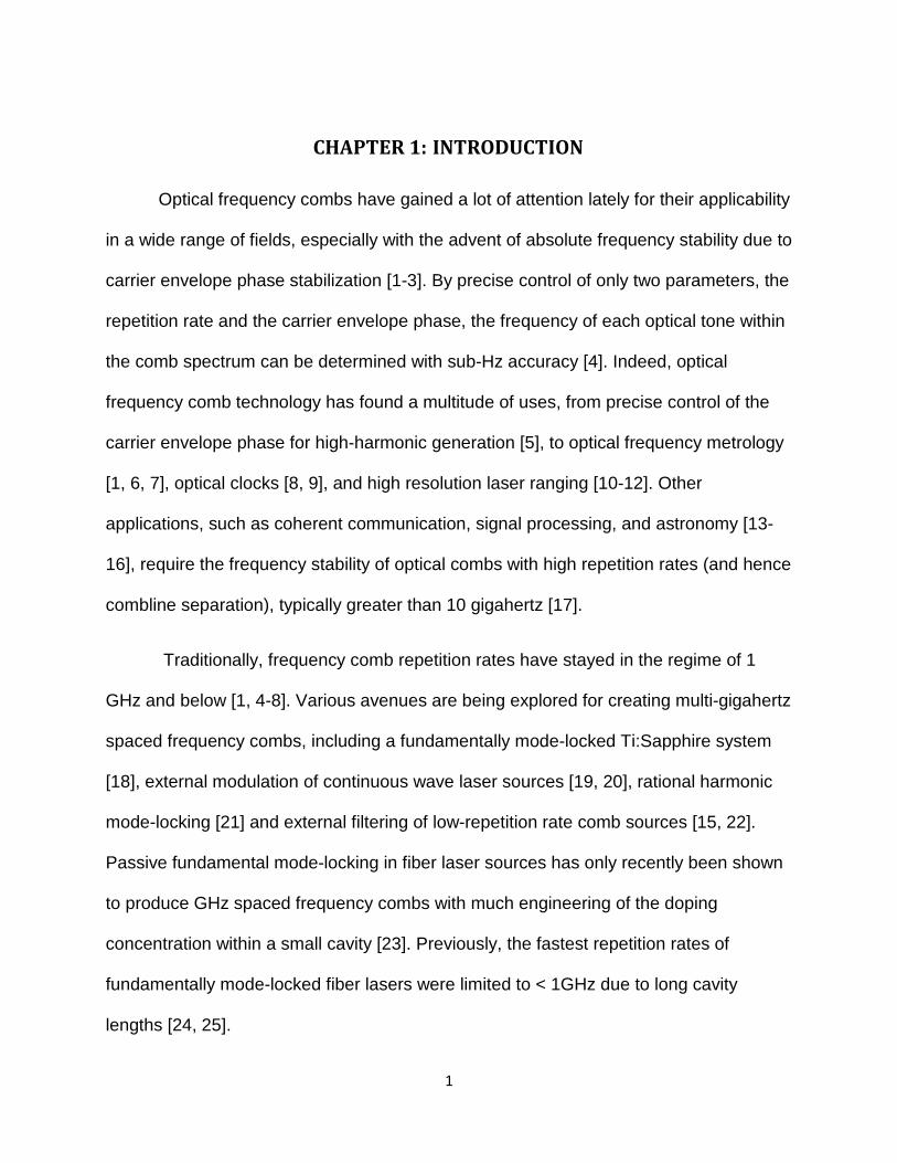
Optical frequency combs have gained a lot of attention lately for their applicability

in a wide range of fields, especially with the advent of absolute frequency stability due to

carrier envelope phase stabilization [1-3]. By precise control of only two parameters, the

repetition rate and the carrier envelope phase, the frequency of each optical tone within

the comb spectrum can be determined with sub-Hz accuracy [4]. Indeed, optical

frequency comb technology has found a multitude of uses, from precise control of the

carrier envelope phase for high-harmonic generation [5], to optical frequency metrology

[1, 6, 7], optical clocks [8, 9], and high resolution laser ranging [10-12]. Other

applications, such as coherent communication, signal processing, and astronomy [13-

16], require the frequency stability of optical combs with high repetition rates (and hence

combline separation), typically greater than 10 gigahertz [17].

Traditionally, frequency comb repetition rates have stayed in the regime of 1

GHz and below [1, 4-8]. Various avenues are being explored for creating multi-gigahertz

spaced frequency combs, including a fundamentally mode-locked Ti:Sapphire system

[18], external modulation of continuous wave laser sources [19, 20], rational harmonic

mode-locking [21] and external filtering of low-repetition rate comb sources [15, 22].

Passive fundamental mode-locking in fiber laser sources has only recently been shown

to produce GHz spaced frequency combs with much engineering of the doping

concentration within a small cavity [23]. Previously, the fastest repetition rates of

fundamentally mode-locked fiber lasers were limited to < 1GHz due to long cavity

lengths [24, 25].

2

Semiconductor-based mode-locked lasers are optimal for producing frequency

combs with multi-gigahertz spacing, due to the short gain recovery time of the

semiconductor [26], with the added benefit of high wall-plug efficiency due to direct

electrical pumping. By incorporating a long external cavity and employing harmonic

mode-locking, higher repetition rates can be achieved while decreasing the optical

linewidth. Low timing jitter and pulse-to-pulse energy fluctuation can be realized as well,

making semiconductor based laser systems ideal for such applications as optical time

domain multiplexing (OTDM) [27] and optical signal processing, including analog to

digital conversion (ADC) [28] and line-by-line pulse shaping [29]. Coherent

communication such as phase shift keying and quadrature amplitude modulation can

also be achieved [30, 31]. In addition, the set of widely spaced phase-locked frequency

components can be exploited for the purposes of optical arbitrary waveform generation

(OAWG) [27, 32] and frequency metrology [33].

Furthermore, the potential for low-noise, high-repetition rate, stand-alone

oscillators offering both optical and radio frequency (RF) outputs through the use of

regenerative mode-locking would be an added benefit to many of the above applications

where cost, weight, size, and increased portability are important. To that end, a stand-

alone system utilizing regenerative mode-locking and injection locking to produce an

optical frequency comb is presented and fully characterized.

1.1 Definitions

‘Frequency comb,’ in the context of this work, is defined as a set of discrete

optical frequency components with a fixed phase relationship relative to one another.

3

Other works require that the laser’s carrier-to-envelope phase (CEP) be actively

stabilized for the output spectrum to be deemed a frequency comb, but this is not strictly

required in the applications outlined here for the laser sources described here.

Therefore, in this document, the term is not restricted to lasers with CEP stabilization.

Harmonically mode-locked lasers (HMLLs), as described in later chapters, exhibit

a unique output spectrum wherein multiple comb groups are interleaved with each

other. The number of these groups is determined by the number of pulses in the cavity

and the integer ratio of the pulse repetition rate to the cavity fundamental frequency.

Each of these groups is referred to as an axial mode group or a supermode. As each of

these groups contains the necessary fixed phase relationship, suppression of all but

one group in the output spectrum will generate a frequency comb, as defined above.

1.2 Applications

Potential applications for high repetition rate mode-locked lasers and frequency

comb sources in both the frequency and time domains are numerous. A few of these

applications are summarized here.

1.2.1 Optical Time Domain Multiplexing

The creation of pulse trains in the multi-gigahertz regime with low pulse-to-pulse

timing jitter is a distinct advantage of external cavity semiconductor-based laser

systems. Communication via optical time division multiplexing (OTDM) utilizes any

number of communication schemes, with the common feature that the low noise pulse

train use is split amongst many users [27], as illustrated in Figure 1.1. The optical

4

pulses are demultiplexed to be modulated for signal transmission by each individual

user. This means that each user will use a ‘pulse train’ at a lower repetition rate equal to

the original repetition rate divided by the number of users. The pulses are then

multiplexed before transmission to the end-receiver [34, 35].

Figure 1.1 Schematic of Optical Time Domain Multiplexing as a utilization of mode-locked laser pulse

trains. Pulses are directed to different modulating signals via an active optical switching mechanism. Each

user then sees a lower repetition rate pulse train on which to impart a signal. Original pulse train is

reconstituted and transmitted to another switch, separated again, and sent to corresponding receivers.

1.2.2 Optical Arbitrary Waveform Generation

Frequency comb sources offer a set of frequency components coherent with

each other, which typically add together to form a periodic set of pulses in the time

domain. However, by spectral demultiplexing and affecting the phase and amplitude of

each individual combline, an arbitrary optical waveform can be created out of the

5

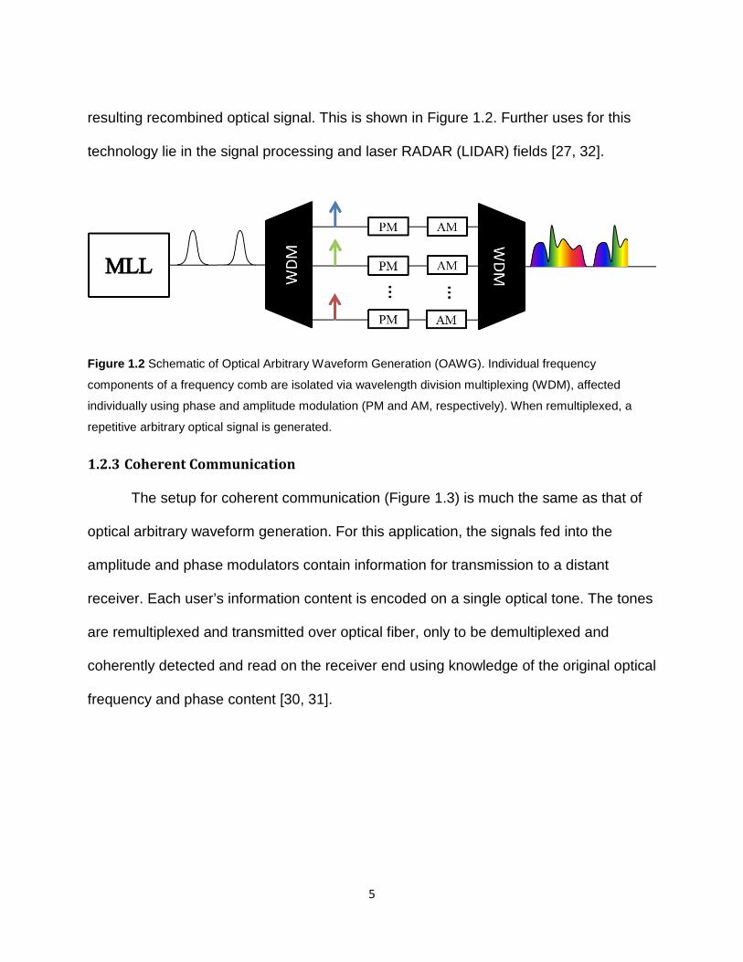
resulting recombined optical signal. This is shown in Figure 1.2. Further uses for this

technology lie in the signal processing and laser RADAR (LIDAR) fields [27, 32].

Figure 1.2 Schematic of Optical Arbitrary Waveform Generation (OAWG). Individual frequency

components of a frequency comb are isolated via wavelength division multiplexing (WDM), affected

individually using phase and amplitude modulation (PM and AM, respectively). When remultiplexed, a

repetitive arbitrary optical signal is generated.

1.2.3 Coherent Communication

The setup for coherent communication (Figure 1.3) is much the same as that of

optical arbitrary waveform generation. For this application, the signals fed into the

amplitude and phase modulators contain information for transmission to a distant

receiver. Each user’s information content is encoded on a single optical tone. The tones

are remultiplexed and transmitted over optical fiber, only to be demultiplexed and

coherently detected and read on the receiver end using knowledge of the original optical

frequency and phase content [30, 31].

6

Figure 1.3 Schematic of an optical coherent communication setup. Each optical frequency component of

a frequency comb is encoded by a unique user’s signal, resulting in a seemingly arbitrary signal sent to

the receiver side, where the individual signals are demultiplexed and received individually.

1.2.4 RF Photonics and Optical Clocks

Building on the principles of optical arbitrary waveform generation, an arbitrary

optical signal can be photodetected to produce arbitrary RF waveforms, shown in Figure

1.4. These waveforms, which contain high instantaneous frequencies up to the

bandwidth of the photodetector used, are often less cumbersome to obtain by this

method than by traditional electronic arbitrary waveform generation [27].

7

Figure 1.4 Conceptual diagram of photonic enabled RF arbitrary waveform generation. An RF waveform

corresponding to the intensity of the arbitrary optical waveform is generated with instantaneous frequency

up to that of the photodetector bandwidth.

Frequency comb sources are being used to push the state-of-the-art of long-term

stability of time standards. By stabilizing the optical frequency components in a comb,

the beating of the optical tones with each other on a photodetector will produce a low-

noise microwave signal [36]. This signal can be used to trigger subsequent modulators

acting on the pulse train, such as in arbitrary waveform generators or ADCs, or can be

combined with electronic counters to produce a stable clock.

An extension of this concept is radio-over-fiber, wherein a few (>2) comblines

with stable frequency separation are modulated and transmitted over optical fiber then

photodetected at the receiver end to produce a transmitted microwave signal [37].

1.2.5 Multiheterodyne Spectroscopy

The burgeoning field of multiheterodyne spectroscopy utilizes a frequency comb

to probe the phase and amplitude information of an unknown multi-wavelength signal

with different periodicity [10, 38-41], as shown in Figure 1.5. This field can also benefit

from easily tunable frequency comb spacing by granting control over the detuning

frequency between the two signal pulse-trains.

8

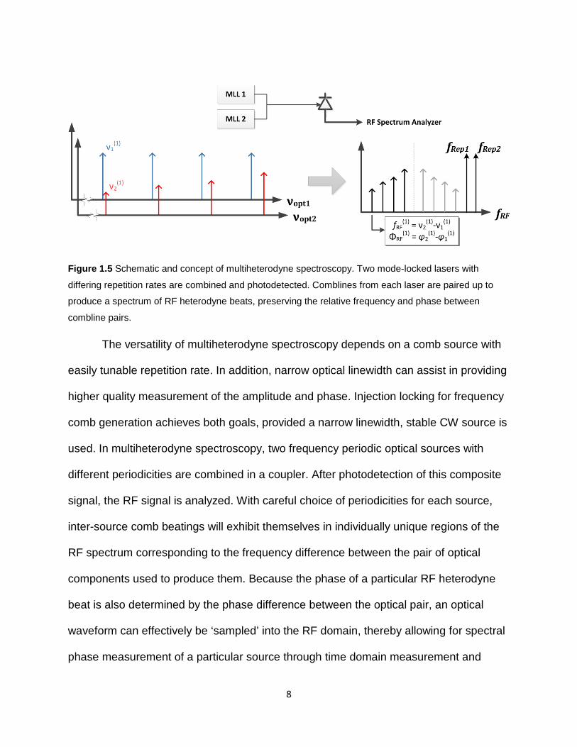
Figure 1.5 Schematic and concept of multiheterodyne spectroscopy. Two mode-locked lasers with

differing repetition rates are combined and photodetected. Comblines from each laser are paired up to

produce a spectrum of RF heterodyne beats, preserving the relative frequency and phase between

combline pairs.

The versatility of multiheterodyne spectroscopy depends on a comb source with

easily tunable repetition rate. In addition, narrow optical linewidth can assist in providing

higher quality measurement of the amplitude and phase. Injection locking for frequency

comb generation achieves both goals, provided a narrow linewidth, stable CW source is

used. In multiheterodyne spectroscopy, two frequency periodic optical sources with

different periodicities are combined in a coupler. After photodetection of this composite

signal, the RF signal is analyzed. With careful choice of periodicities for each source,

inter-source comb beatings will exhibit themselves in individually unique regions of the

RF spectrum corresponding to the frequency difference between the pair of optical

components used to produce them. Because the phase of a particular RF heterodyne

beat is also determined by the phase difference between the optical pair, an optical

waveform can effectively be ‘sampled’ into the RF domain, thereby allowing for spectral

phase measurement of a particular source through time domain measurement and

9

phase unwrapping [38]. The reference also demonstrates passive measurement of

relative phase between two signals. This is achieved by correlation of simultaneous

multiheterodyne measurements with a common local oscillator. This is beneficial in, for

example, measuring the relative phase between input signals at two detectors in a

sparse synthetic aperture radar system.

1.2.6 Photonic Analog-to-Digital Conversion

Pulses with ultra-low timing jitter from high-repetition rate mode-locked lasers

with ultra-low amplitude and phase noise can be utilized to sample an RF waveform and

convert the sampled points into a digital code representing the amplitude at well-defined

time intervals such that the analog signal can be reconstructed at a receiver. This is

done so that the signal may be transmitted in the digital domain with less loss of fidelity.

A schematic of photonic sampling for ADC is shown in Figure 1.6. It becomes apparent

from the picture, then, that timing jitter on the input pulses will result in sampling the

waveform at the wrong point in time, and associating an incorrect amplitude value with

that time bin when reconstructing the signal. Similarly, pulse intensity fluctuations into

the modulator with a constant transfer function will be mistaken for an erroneous

amplitude value of the signal. A review of photonic ADC can be found in reference [42].

Photonics can also assist in sampling short bursts of signals at higher

instantaneous frequencies than conventional electronics by utilizing an optical time-

stretched architecture [43, 44]. An example of a semiconductor-based HMLL tailored to

this application with low noise and low repetition rate, is presented in references [45-47].

10

Figure 1.6 A generalized picture of photonic enabled analog-to-digital conversion wherein mode-locked

laser pulses with ultra-low timing jitter and pulse-to-pulse energy fluctuations are modulated using the

signal to be converted. Each pulse samples the waveform at a set interval and its amplitude value can

then be independently recorded in digital format.

11

CHAPTER 2: HARMONICALLY MODE-LOCKED LASERS

In the introduction, several photonic applications were presented which value

frequency combs with great stability, narrow optical linewidth, and wide combline

spacing and high pulse repetition rates. In order to achieve low optical linewidths (~100s

of kHz) from laser cavities, a long optical storage time is achieved through long fiber

cavity lengths. However, high pulse repetition rates are also desirable while maintaining

long optical cavities (and therefore a low fundamental cavity frequency, ν0),

necessitating the employment of harmonic mode-locking in laser systems.

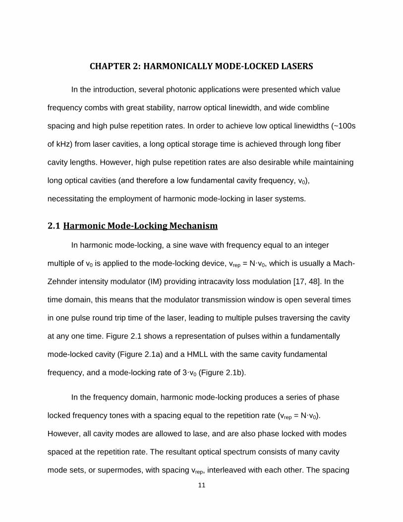
2.1 Harmonic Mode-Locking Mechanism

In harmonic mode-locking, a sine wave with frequency equal to an integer

multiple of ν0 is applied to the mode-locking device, νrep = N·ν0, which is usually a Mach-

Zehnder intensity modulator (IM) providing intracavity loss modulation [17, 48]. In the

time domain, this means that the modulator transmission window is open several times

in one pulse round trip time of the laser, leading to multiple pulses traversing the cavity

at any one time. Figure 2.1 shows a representation of pulses within a fundamentally

mode-locked cavity (Figure 2.1a) and a HMLL with the same cavity fundamental

frequency, and a mode-locking rate of 3·ν0 (Figure 2.1b).

In the frequency domain, harmonic mode-locking produces a series of phase

locked frequency tones with a spacing equal to the repetition rate (νrep = N·ν0).

However, all cavity modes are allowed to lase, and are also phase locked with modes

spaced at the repetition rate. The resultant optical spectrum consists of many cavity

mode sets, or supermodes, with spacing νrep, interleaved with each other. The spacing

12

between adjacent supermode sets, then, is the fundamental frequency of the cavity, ν0.

Figure 2.1c and Figure 2.1d show the frequency domain representation of the optical

output of a fundamentally mode-locked laser and a HMLL, both with the same cavity

length.

Figure 2.1 Fundamental (a) versus harmonic (b) mode-locking in the time domain for laser cavities of the

same length showing multiple pulses traversing the harmonically mode-locked cavity. Representations of

the spectral output in the fundamental (c) and harmonic (d) mode-locking cases showing the presence of

optical supermode sets in a HMLL. The Semiconductor Optical Amplifier (SOA) gain media are shown as

red triangles and the IMs are shown in the lower part of the cavities, along with the input sine wave to the

respective modulators. In this example the HMLL contains three pulses traversing the cavity.

2.2 Sources of Noise in Harmonically Mode-Locked Lasers

By its very nature, a laser gain medium can spontaneously emit light which can

then be amplified and contribute significantly to the noise of any laser system. In

particular, semiconductor gain media have fast electron recombination rates, and laser

13

noise spectral features due to this effect can occur at frequencies well into the gigahertz

[26]. This amplified spontaneous emission (ASE) is also necessary in starting the lasing

process, and frequencies of light which are resonant with the cavity constructively

interfere and are amplified, regenerating the signal at those frequencies. Long fiber

cavities will increase the cavity photon lifetime, narrowing individual resonances and

therefore the laser linewidths [49]. This linewidth narrowing has been shown to

significantly improve phase and amplitude noise in mode-locked lasers, by reducing the

‘knee frequency’ of the power spectral density [50], the frequency in a noise power

spectral density plot where the noise begins to roll-off precipitously.

One significant noise feature unique to HMLLs is the supermode noise spur

(SNS), which occurs due to the beating between adjacent yet uncorrelated laser cavity

modes. This lack of correlation is due to the harmonic nature of the intracavity mode-

locking mechanism and leads to pulse-to-pulse amplitude fluctuations and timing jitter,

both detrimental for the aforementioned applications [50, 51]. This feature is present in

RF and noise spectra at multiples of the cavity fundamental frequency up to the

repetition rate of the laser system. In order to improve the phase and amplitude noise

performance, all supermode sets but one should be suppressed. Two methods are

currently employed to achieve this suppression: an intracavity etalon with a free spectral

range (FSR) equal to that of the desired repetition rate of the laser [52-55] and single

frequency optical injection into the MLL cavity [56-58]. The latter method works by

preferentially adding power to one supermode set, while the non-selected supermode

sets are deprived due to gain depletion. This work will focus on the latter method.

14

CHAPTER 3: INJECTION LOCKING OF OSCILLATORS

Injection locking of an oscillator was first observed by Christian Huygens in 1865.

He noticed the synchronization of two pendulum clocks that were hung in close

proximity to each other [59, 60]. Since that time, the field of injection locking in

oscillators has been more rigorously studied in electrical oscillators [61, 62] and also in

laser oscillators [63, 64]. Some basic concepts are summarized here for the benefit of

introduction to the research presented.

A laser can be thought of as an amplifying interferometer with regenerative gain.

As such, the gain at some frequency offset from a particular optical mode is non-zero.

This allows for a weak optical signal coupled into the cavity at a frequency near a

resonant optical mode to see gain. When the injected frequency comes close to the

center of the resonant cavity mode – within a certain locking range – the cavity begins

to lase at the injected frequency, resulting in a ‘frequency pulling’ effect. Figure 3.1

illustrates this frequency range relative to the resonance window of the optical cavity.

This effect is due to the injected signal experiencing increasing gain, depriving the

previously lasing cavity mode of that gain. In this regime of operation, the laser is said to

be injection locked [65]. The injected mode now lases exclusively at the injection

frequency, maintaining the spectral quality of the injection seed due to gain suppression

of other frequencies. In order to maintain this amplification of an off-resonant frequency,

the cavity imparts a phase shift on the injected signal, which will be discussed in some

detail later. Within the locking range, as depicted in the figure, the amplitude is relatively

clamped and roughly equivalent to the sum of the free-running slave laser power and

15

the injected power. When injecting outside the locking range, both signals will coexist -

the master signal may see some gain, and be slightly amplified and may ‘pull’ the

oscillator frequency as described by Razavi [66], but will not overtake the lasing mode,

meaning the free-running slave signal magnitude will be mostly unaffected.

Figure 3.1. A slaved cavity resonance and its relevant injection locking properties. The locking range is

demonstrated by the vertical cyan lines, as well as the injection lock phase limits of ± π/2, while the

regenerative gain curve of the resonance (solid blue lines) is shown versus optical frequency.Within the

locking range, the normalized output power is clamped, approximated by a higher order Gaussian (green

circles). The normalized transmission of a passive cavity, defined by the real part of the Airy function, is

shown in solid green. The phase shift that an injected tone experiences as it moves across the resonance

is shown in red and is shown as an arcsin shape extending from π/2 to - π/2 over the locking range.

16

While the phase outside the injection locking range is unknown, it is assumed in

this manuscript and in the simulations in later sections to be that of a passive cavity,

defined by the Airy function. This assumption is also mitigated by the Airy function

having a slowly varying phase at large detuning frequencies away from each

resonance.

3.1 Applications of Injection Locking

The injection locking technique is used to synchronize or control the frequency

output of a laser [67, 68]. It can be used in power amplifiers to take advantage of high

gain in regenerative amplifier systems while maintaining the spectral qualities of a less

intense master oscillator. Injection locking is also utilized in optical communication

schemes to impart phase-shift keying signals via semiconductor cavities where small

changes in the injected current rapidly shift the cavity resonance position relative to a

steady injection frequency. This provides advantages in both the necessary peak-to-

peak voltage and in modulation frequency, which can reach into the tens of

gigahertz.[69-74]. A similar embodiment utilizes the arcsin shaped phase shift

characteristic in injection locking (which will be discussed in the next section) within a

Mach-Zehnder style modulator for inherently linear intensity modulation [75, 76].

In a multi-wavelength slave laser, injection locking has been shown to lock a

mode-locked laser quite effectively, with the output being a set of phase-locked

frequency components anchored by the injection frequency [56, 77]. The mode-locking

mechanism, whether passive or active, locks the phases of the frequency components,

17

producing a comb, while injection locking synchronizes the optical frequency to the

injection seed frequency, stabilizing the comb.

In HMLLs, injection locking has the added benefit of suppressing the unwanted

optical supermodes through gain suppression. This not only stabilizes the optical

frequency of the resultant comb output, but also reduces the optical linewidth [78], the

relative timing jitter of the laser, as well as the pulse-to-pulse energy fluctuation [57].

3.2 Semiconductor Cavity Dynamics of Injection Locking

As stated earlier, a phase shift is imparted on the injection frequency during

injection locking, which is dependent on the detuning frequency from the center of the

free-running slave cavity resonance, as depicted in Figure 3.1. Adler first described the

behavior of injection locked electrical oscillators and the arcsin shape of the phase

imparted on the injection locked output frequency for small injection powers [79]. This

phase shift and its resulting affinity for better oscillator injection locking at negative

detuning frequencies is described using phasor diagrams [66, 70]. Furthermore,

Paciorek [80] explored both the time necessary to achieve injection locking as well as

the behavior of the phase across the resonance when the injected power approached

that of the free-running slave laser output. In this case, the phase curve can approach

arctangent, what one would expect in a cavity with no gain. It is assumed that outside of

the locking range, the phase imparted on an injected frequency is also similar to that of

the passive cavity, arctangent as a function of detuning frequency, since there is little

interaction between the oscillations of the master and free-running slave signals.

18

Due to fast carrier and gain dynamics in semiconductor lasers, the phase

response of a slave laser cavity with semiconductor gain is somewhat more complicated

than that of other gain media. Direct electrical pumping creates free carriers (electrons

and holes) in the semiconductor material. Due to the availability of these carriers and

their affinity for recombination, the index of refraction is heavily dependent on the

population of such carriers in the material. Real-time fluctuations in input light intensity

will understandably lead to rapid changes in the carrier density and therefore index of

refraction. This results in a coupling between intensity and phase noise in

semiconductor gain media, first introduced by Henry [81] in 1982. The first indication of

this effect was in measuring the linewidth of semiconductor lasers, which did not come

close to that predicted by the Schawlow-Townes fundamental limit for laser linewidth

[49]. The effect was therefore dubbed the linewidth enhancement factor (LEF), denoted

by α in equations and commonly referred to as the alpha factor.

19

Figure 3.2. Semiconductor laser cavity resonances with non-zero alpha parameters, shifting resonance

phase downward and broadening the injection locking range. Note the difference in frequency scale

between figure a) and figures b) and c).

20

The linewidth enhancement factor effect in semiconductor lasers has since been

well studied and several groups have used the model developed by Henry to study

various characteristics of injection locking in semiconductor lasers [69-74, 76].

While the LEF was found to increase the natural linewidth of semiconductor

lasers by (1+ α 2), it also affects the behavior of injection locking in two significant ways.

First, the locking range half-width is broadened by the square root of the same factor,

resulting in a locking half-width of:

∆𝜔𝐿 = 𝑓𝐷𝐸1𝐸0√1 + 𝛼2 ( 1 )

where ΔωL is the locking half-width, fD is the cavity longitudinal mode spacing, and E1/E0

is the electric field ratio [82]. This is demonstrated in Figure 3.2a-c for alpha parameters

1, 1.75, and 3. This is in contrast to that of Figure 3.1, where the alpha parameter is set

to zero.

Another significant effect of the LEF is a shift in the phase incurred across the

injection locking range downward by a factor of atan(α), resulting in the phase across

the resonance being defined by the following equation:

𝜑0 = − asin(𝜔 −𝜔0) − atan (𝛼) ( 2 )

This is also shown in Figure 3.2a-c for the alpha parameters considered there.

As stated earlier, this phase shift is a function of the slaved laser cavity compensating

for a lasing mode which is off resonance, and hence the phase at center of the

resonance (for zero alpha) is zero. The limit, however, to the ‘tolerance’ of the slaved

21

laser is when the phase incurred reaches ± π/2. As shown in the figure, this leads to a

portion of the injection locking range with values outside of those limits. In this region,

the injection locking dynamics become quite unstable [83]. As the locking range and

hence unstable region are dependent on the injection electric field ratio, this region

understandably grows with increasing injection power[76, 82]. An intuitive picture of the

carrier dynamics involved in this affinity for injection locking at negative detuning

frequencies and instability for positively detuned external injection is explained

succinctly by Lang in 1982 on page 982 of [83]:

With light injection, the laser output increases in general, and the excited carrier

density in the active region decreases correspondingly. Decrease in the carrier

density increases the refractive index of the active region which results in the

lowering of the cavity resonance frequency. Therefore, the optimum locking can be

achieved when the injected light frequency ν coincides with the resonance

frequency ω which is downshifted by the light injection.

A secondary consequence of the LEF affecting both the locking range and

stability region is a change in total amplitude of the injection locked frequency across

the locking range, as a function of both detuning frequency and injection electric field

ratio. While this effect may have significant implications for some injection locking

applications [76], such small changes in resultant power are not as important in this

work, as the detuning frequency will be stabilized in the final embodiment of the system.

22

CHAPTER 4: LASER CAVITY STABILIZATION VIA POUND-DREVER-HALL METHOD

4.1 Pound-Drever-Hall Cavity Stabilization Overview

The Pound-Drever-Hall (PDH) method of cavity stabilization is used in many

variations to actively long-term stabilize an optical cavity, such as a Fabry-Pérot etalon,

relative to a laser frequency or vice versa [84]. Based on previous methods in electrical

oscillators [85], the technique exploits the existence of a phase shift across each

resonance of the optical cavity, which is, in the classic case, an etalon. By detecting the

phase shift of a frequency coupled into the etalon, the frequency offset between the

center of the resonance and the injected frequency can be determined, leading to a

differential error signal. By actively changing either the injected optical frequency or the

absolute position of the etalon cavity resonance, the etalon and injected frequency can

be stabilized relative to one another [86].

Continuous wave (CW) injection (CHAPTER 3) will pull the frequency of a laser

system when weak injected light is within the locking range of the cavity resonance.

Environmental effects cause significant length fluctuations in the long fibers used in

external cavity semiconductor lasers. Therefore, a feedback technique becomes

necessary to compensate for these fluctuations and keep the injection frequency within

the locking range. In the modified PDH method used in this work, the mode-locked laser

cavity serves as the optical cavity being probed, as opposed to a passive optical cavity

used in the conventional embodiment of the PDH method. A stable, commercially

available laser operating at 1550 nm is used as the reference to which the cavity modes

23

will be locked, while also serving as the injection seed light. The modified PDH method

maintains the injection locked state and therefore stabilizes the mode-locked laser

output long-term. Similar sideband scheme stabilization has been performed in pulsed

lasers [87] and more recently in Q-switched laser designs [88, 89], though the work

featured here is the first use for the generation of frequency combs through injection

locking of mode-locked oscillators.

Within the locking range, the laser cavity will also impart a phase shift on the

injected tone. According to Adler [79], for injection locked oscillating systems with gain,

this phase is an arcsin shape, compared to the arctan phase profile of an etalon

resonance. The cavity phase shift around a cavity resonance and the locking bandwidth

are shown in Figure 3.1.

In order to detect this phase shift, the injection laser, at frequency νinj, is phase

modulated to produce sidebands at νinj±νPM prior to injection into the cavity. Additional

injection and lasing of these phase modulation sidebands could result in unwanted

spectral components and additional noise in the laser output. Therefore the sidebands

are created at such spacing that they will not be resonant with the optical cavity when

the injection frequency is within the locking range of a cavity mode. Figure 4.1 shows

the relative placement of the phase modulation sidebands when coupled into the

harmonically mode-locked cavity.

24

Figure 4.1. Representation of the injection seed frequency and phase modulation sidebands injected into

a HMLL. Note that the phase modulation sidebands are not resonant with the optical cavity when the

injection seed frequency is within a cavity resonance injection locking range.

As the cavity resonance is shifted relative to the three injected tones due to an

induced change in optical cavity length, the central tone, νinj, experiences the

aforementioned phase shift, while the sidebands do not. By photodetecting the output of

the laser with the three tones present in the signal, then mixing the signal with the

original phase modulation frequency in quadrature, the sum and difference frequencies

are produced. Using a low-pass filter (LPF), the DC signal is isolated and, within the

locking range, is a differential signal proportional to the difference between the injected

frequency, νinj and the center of the cavity mode resonance, νR. A proportional-integral

controller (PIC) is employed, using the linear portion of the error signal to feed back into

an intracavity fiber stretcher, thereby allowing for long-term stabilization of the optical

cavity relative to the injection seed frequency.

25

4.2 Modified Pound-Drever-Hall Stabilization Error Signal Simulation

As will become evident in this and subsequent chapters, the experimentally

obtained error signals used to stabilize the injection locked frequency comb source are

the result of vastly different phenomena as that of the conventional PDH error signal,

starting with an arcsin phase shift across a cavity injection locking range as opposed to

arctangent in a passive etalon case. This and other phase and amplitude effects of

injection locking are studied and simulated in the following section to further understand

the origin of the injection locked modified PDH error signal shape. The PDH error

signals for both passive and injection locking cases are simulated in MATLAB

simulation software. A version of the programming code can be found in APPENDIX C.

4.2.1 Conventional Pound-Drever-Hall Error Signal

To begin with, a more detailed understanding of the conventional PDH error

signal must be presented. As stated in the chapter introduction, PDH stabilization was

first proposed by Drever and Hall [84] based on electronic methods by Pound [85]. Yet

an excellent review and explanation of the topic is found in a paper by Eric Black [86].

Conventional PDH stabilization exploits the arctangent phase shift across a cavity

resonance, shown in Figure 4.2b to detect a frequency detuning between an injected

frequency and the resonance center frequency. In order to perform this, PM sidebands

are placed on the injected frequency, one sideband having characteristic opposite

phase from the other two. This means that when the center, or carrier frequency phase

is unchanged, under ideal conditions, photodetection would lead to no signal, as the

beating between the positive sideband and the carrier and the negative sideband and

26

carrier would cancel out each other. These sidebands are placed at a sufficient enough

frequency as to lie outside of the cavity resonance while the center frequency is

interacting with it, thereby acting as a phase reference in seeing near ±π phase which is

also slowly varying. All three frequencies are injected into the passive optical cavity and

the reflection is observed and photodeteced. As the carrier frequency sweeps across

the resonance, it incurs the arctan phase shift according to the Airy function [86],

thereby making the beat signal of all three tones after photodetection nonzero for all

nonzero detuning frequencies. At the center of the cavity resonance, zero phase shift

and zero amplitude of the injected carrier frequency are seen as it experiences full

transmission through the cavity. Furthermore, the sign of the phase incurred flips as it

passes from one side of the resonance to the other, and the signal grows as the

reflected power of the carrier frequency increases with greater positive or negative

detuning. After reflection and photodetection, the phase modified beating at the PM

frequency is downconverted to low frequencies (direct current or DC) via mixing with the

original PM signal. Typically the two signals are mixed in quadrature, yet different RF

phases significantly affect the overall shape of the signal obtained. Higher order terms

are low-pass filtered out.

27

Figure 4.2. a) Conventional PDH Error Signal derived from a cavity with R = 0.99 and PM frequency of

1.13*FSR. b) Passive FPE cavity normalized transmission (blue) and phase (green), according to the Airy

function governing passive cavity behavior.

As a result of this process, the center region of the conventional PDH error signal

results in a differential signal used to stabilize the optical frequency relative to the

passive cavity resonance. The entire error signal is shown in Figure 4.2a, where the PM

frequency is sufficiently outside of the locking cavity resonance or any other resonance

of a periodic optical element such as a Fabry-Pérot Etalon. The large feature in the

center of the error signal, as alluded to before, is the result of the carrier frequency

28

being swept past the cavity resonance. The smaller side features result from the PM

sidebands sweeping through the cavity as well, experiencing the same phase shift and

beating with the carrier frequency at the PM frequency and being downconverted by the

PDH electronics. As the side features are sufficiently distinct from the center feature, yet

not completely independent, this type of signal shape is colloquially referred to as the

‘Batman’ error signal for its double spikes just to the left and (reversed) to the right of its

center.

4.2.2 Simulated Cavity Resonances

The simulated slaved cavity resonance is similar to that described in CHAPTER

3, yet with multiple resonances separated by an FSR of 100 MHz. In the simulation, an

electric field ratio, the ratio of the injected electric field magnitude to that of the naturally

occurring electric field in the slave resonance, is specified, as well as a modulation

index to determine the power in first order and second order sidebands of the PM

signal. Based on these values and equation (1) the locking range is determined for the

center resonance as well as two others on either detuning side, as the PM sidebands

will injection lock those resonances and hence see similar asin phase shifts, affecting

the error signal shape. Equation (2) is used to numerically specify the phase across

each resonance. A higher order Gaussian function is used to specify the amplitude

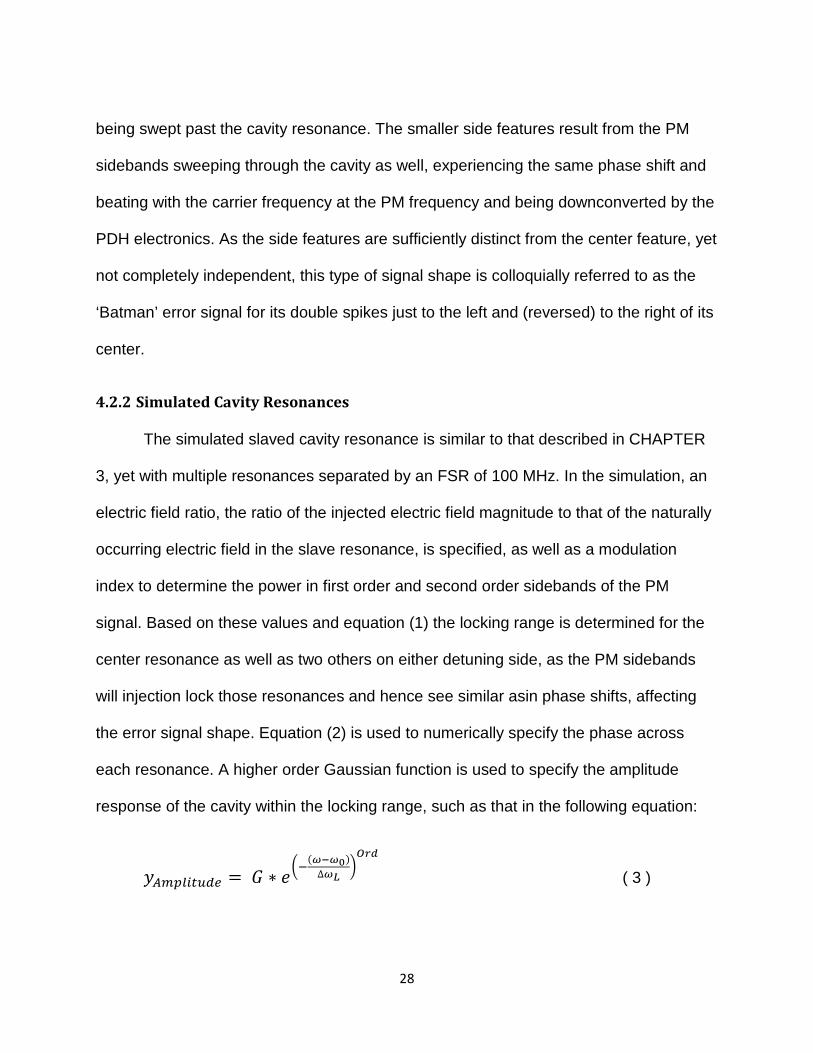
response of the cavity within the locking range, such as that in the following equation:

𝑦𝐴𝑚𝑝𝑙𝑖𝑡𝑢𝑑𝑒 = 𝐺 ∗ 𝑒�−(𝜔−𝜔0)∆𝜔𝐿

�𝑂𝑟𝑑

( 3 )

29

where G is the gain of the simulated cavity, ω is the detuning frequency, ω0 is the cavity

resonance center, ΔωL is the locking half-width, and Ord is the Gaussian order. While

the conventional PDH relies on the reflection signal of a cavity, which goes to zero at

the resonance center, it has been found empirically in the injection locked frequency

comb generation system that this is not the case at the ‘reflection’ output used (the

previously unused output of the IC), and therefore the amplified transmission from

injection locking theory is used in the simulation, which, as stated before, is best

approximated by this super-Gaussian function. Various orders between 4 and 60 are

used to sharpen the edges of the locking range amplitude. Amplitude and phase

characteristics of the relevant optical cavities are shown in Figure 4.3, below.

Figure 4.3. Cavity amplitude and phase response within injection locking ranges for the center resonance

and two nearest neighbor resonances, which PM sidebands interact with while the carrier is near zero

detuning.

30

Outside each resonance, the phase and amplitude are approximated by the

passive cavity Airy function:

𝑅𝐴𝑖𝑟𝑦 = 𝑅∙𝑒2𝜋𝑖(𝜔−𝜔0)

𝐹𝑆𝑅 −1

1−𝑅2∙𝑒2𝜋𝑖(𝜔−𝜔0)

𝐹𝑆𝑅 ( 4 )

where R is the mirror reflectivity. While the exact nature of amplitude and phase

behavior is not known in this region for the present system, the small amplitudes and

slowly varying phases at these large detuning frequencies from each cavity resonance

make this an acceptable assumption in the simulation.

4.2.3 Modified Pound-Drever-Hall Simulations

The simulation then computes PDH error signal for the set of cavities with the

injection electric field ratio, phase modulation index, alpha parameter, mirror reflectivity,

free spectral range, Gaussian order, and gain parameters specified. Other values in the

simulation which are set up to be appropriate fitting parameters for matching simulated

signals to experimentally obtained signals are the PM frequency, RF mixing phase in

the PDH calculation. It is worth mentioning that previously named injection parameters

such as the electric field ratio and phase modulation index which define the amount of

injected power, and hence the locking range and phase excursion of each resonance

are extremely important in the fitting of the simulated error signals.

Experimentally obtained error signals were chosen to compare to simulation and

were plotted with simulated results to obtain a visual fit of the signals while adjusting the

aforementioned parameters. The first signal used, shown in Figure 4.4, was chosen for

31

its clearly discernible features, but is not usable for actual stabilization of the cavity, as a

differential feature does not exist at the appropriate locking point. For appropriate

context, the same error signal is used for exploration of injection locking qualities in

Section 5.2.3. In order to match the simulated and measured error signals, the

simulated cavity FSR was maintained at 100 MHz and the experimentally obtained error

signal time/frequency scale is adjusted to fit the simulated features that arise, since the

measured error signal is arbitrarily based on the magnitude of the cavity sweep at the

time it was taken. In addition, the amplitude, vertical offset, and time offset of each

signal were adjusted accordingly. Also of note is that the measured error signal is

reversed in the horizontal scale, as it was determined that the direction of cavity sweep

was such that ‘earlier’ times on the oscilloscope trace corresponded to positive cavity

detuning and ‘later’ times corresponded to negative frequency detuning from the

resonance of concern.

The simulated PM frequency was set at one FSR plus a fraction for ease of

comparison and specification in terms of the experimental parameters. Correspondingly,

the experimental PM frequency and cavity FSR were noted at ~700 MHz and ~46.9

MHz, respectively, and the ratio calculated between them. The fractional remainder plus

one simulation FSR was used as the initializing value for simulating the error signal. The

measurement of cavity FSR is based on an estimation between the SNSs in the RF

spectrum. As this is representative of the beating of optical cavity modes, which are not

evenly spaced across the spectrum, the measurement cannot be exact, and therefore

some leeway in the fitting of the PM frequency in the simulation is allowed.

32

Figure 4.4. Comparison of experimentally obtained error signal (blue, PM frequency ~ 15.047*FSR) to

simulated error signal (red) with the parameters shown. The multiple cavity amplitude responses are

shown in green, while their phase responses are shown in cyan.

Figure 4.4 shows the best fit for the simulated error signal to the experimentally

obtained error signal along with simulation fitting parameters and experimental

conditions. As shown, there is good agreement in the middle of the signals, with odd

symmetric parabola-like features on either side of the resonance center. This

corresponds to the carrier frequency seeing a slowly varying phase in the middle of the

shifted asin, while one sideband sees a similar slowly- or non-varying phase while the

other first order sideband is quickly swept through the asin phase of its corresponding

33

resonance. For example, while the carrier is slightly negatively detuned (by exactly the

PM frequency from the next positive resonance), it sees the phase displayed at that

frequency. Meanwhile the first order negative sideband is far out of its resonance,

seeing the slowly varying Airy function phase, and the first order positive sideband is

swept through its corresponding resonance, incurring a large and quickly varying phase

sweep. The mode beating between the three tones is detected in the PDH scheme,

translating into the sharp error signal feature shown at a slight negative detuning from

the center. A similar process happens at the same positive detuning frequency, albeit

with opposite phase, since the negative sideband has opposite phase as that of the

positive from the phase modulation process.

A look at larger detuning frequencies reveals less agreement with the

experimental error signal, but some similarities can be identified. For instance, what

appears as a single cycle of a triangle waveform with 50% duty cycle appears between

subsequent locking signals of the measured error signal. The simulated signal appears

to approximate, albeit poorly, half of each of these features, with opposite polarity at

positive and negative detuning. However, further analysis reveals that the other polarity

of each of these features is contained in the next injection locked resonance’s error

signal. This is demonstrated in Figure 4.5, where the measured and simulated error

signals are plotted, along with a copy of the simulated signal horizontally shifted by one

positive FSR and a copy shifted by one negative FSR. Note the position of the largely

detuned features relative to one another and, in combination with the original non-

34

shifted simulated signal, their approximation of the triangle waveform seen in the

experimental error signal.

Figure 4.5. Comparison of experimentally obtained error signal (blue) to simulated error signal (red), as

well as copies of simulated signals shifted by one FSR in the positive detuning direction (pink) and

negative detuning direction (black) to illustrate the origin of triangle waveform features between each

cavity resonance.

This feature is thought to arise when the carrier is experiencing the rapid phase

changes at the edge of the asin curve at the same time that one of the sidebands is

experiencing a similar rapid phase shift at the opposite end of the asin curve. Due to the

35

large injection electric field ratios, the edges of the defined phase within the injection

locking bandwidth of the center resonance may not be well approximated, as intimated

before. Via Paciorek [80], the edges of the asin phase may start to exhibit atan

behavior, which could lead to a better approximation of the shape of these largely

detuned features.

The necessity of this horizontal shift for visual fitting purposes highlights a

weakness of this method of simulating the error signal, namely that it only accounts for

the carrier injection locking one particular resonance. As the sweep is applied of the

cavity resonance relative to the injection frequency, each resonance it sees is treated as

the ‘center’ resonance for subsequent error signals seen in an oscilloscope trace (not

shown in any signals here). When this is considered, it becomes likely that the triangle

waveform features could be resulting from independent interleaved features from

contiguous error signals. This seems to be confirmed by adjusting the PM frequency

and observing each triangle waveform devolve into two separate oppositely-moving

features.

A further revelation of these interleaved waveforms and the calculated locking

range obtained through the error signal comparisons is that the locking ranges for

subsequent resonances are overlapping. This implies that, at the electric field ratios

considered, the laser is always within the locking range of at least one cavity resonance,

and is therefore always ‘injection locked’. However, only certain positions near the

center of the unlocked resonance provide sufficient frequency comb bandwidth by

36

injection locking many modes across the lasing bandwidth via the mode-locking

mechanism and spaced at the repetition rate of the HMLL.

Figure 4.6. Comparison of realistic locking signal to simulation results. Visual fitting was able to closely

approximate either a) the center features including the differential features used for feedback stabilization,

or b) the overall shape of the error signal.

37

Since the error signal used was configured so as to make it unsuitable for

realistic PIC locking (i.e. with a differential signal at the appropriate locking region of the

error signal), a second error signal was compared to simulation, and fitting parameters

adjusted to approximate the error signal. The result is shown in Figure 4.6a, with good

agreement in the center, including both sharp features at small detuning frequencies, as

well as the differential portion used to lock the laser, highlighted in the figure, and the

slight ‘hesitation’ feature at zero detuning. However, the largely detuned features show

less visual agreement than the previous example. Adjusting the parameters for a better

overall fit, however, did not account for the differential signal near zero detuning

frequency which is used for feedback stabilization, as shown in Figure 4.6b.

38

CHAPTER 5: CW INJECTION LOCKING OF AN ACTIVELY MODE-LOCKED LASER

As an embodiment and test of the principles outlined in the previous chapters, a

laser system was constructed to generate a GHz-spaced frequency comb output using

an injection locked HMLL. For this particular system, the comb spacing desired was

nominally 2.5 GHz.

5.1 Actively Mode-Locked Injection Locked Laser Setup

Figure 5.1 shows the setup of the laser system for the injection locking of an

actively mode-locked laser with the modified PDH feedback loop [90, 91]. The cavity

consists of a semiconductor optical amplifier (SOA) within a fiberized ring cavity. A

Mach-Zehnder intensity modulator (IM) is used for mode-locking at 2.5 GHz, the 42nd

harmonic of the cavity fundamental frequency, ~60 MHz.

A fiber phase shifter is placed in the cavity for fine adjustment of the cavity

length, while a free-space variable optical delay allows for course adjustment of the

cavity length to directly control the repetition rate. A bandpass filter is utilized to force

lasing at the injection seed frequency as well as an isolator to ensure unidirectional light

propagation. Polarization controllers and dispersion compensating fiber are included for

additional control of the spectral output, and an injection coupler and output coupler are

used to couple light in and out of the cavity. The laser system produces 2-3 mW

average power with an injection locked pulsewidth of ~22 ps FWHM. The optical cavity

is also enclosed within a thermally insulated box to minimize the effects of

environmental fluctuations on the cavity length.

39

Figure 5.1. Laser system schematic of actively mode-locked injection locked laser with long-term

feedback. BPF: Optical Bandpass Filter; DBM: RF Double Balanced Mixer; DCF: Dispersion

Compensating Fiber; FPS: Fiber Phase Shifter; IC: Injection Coupler; IM: Intensity Modulator; IPM:

Injection Power Monitor; IS: Isolator; ISL: Injection Seed Laser; LPF: RF Low Pass Filter; OC: Output

Coupler; PC: Polarization Controller; PD: Photodetector; PIC: PI Controller; PM: Phase Modulator; PS:

RF Phase Shifter; RFA: Low Noise RF Amplifier; SOA: Semiconductor Optical Amplifier; VOA: Variable

Optical Attenuator; VOD: Variable Optical Delay

The injection arm consists of the injection seed laser, a commercially available

fiber laser with an output wavelength of ~1550.1 nm and a linewidth on the order of a

few kHz. An isolator is employed to protect the laser from back reflection. A phase

modulator produces the phase modulation sidebands on the injection frequency for the

modified PDH feedback scheme, and a variable optical attenuator is used for control of

the injection power. Half of the remaining power is coupled out for monitoring, resulting

in ~5 μW of injected power into the laser cavity. Two polarization controllers are also

40

employed to control the polarization of the injected light, which is ultimately coupled into

the cavity using a 90/10 ratio fiber coupler. A signal near 500 MHz is used for the phase

modulation in the PDH feedback scheme, though not at a rate that will produce cavity

resonant sidebands.

5.2 Laser Preparation for Frequency Comb Generation

The injection locked frequency comb source is created out of a harmonically

mode-locked laser. Therefore, the first operational step in creating the frequency comb

is to mode-lock the laser. While specific parameters for mode-locking may be found in

other sections, the information is repeated here for a more complete picture of the

frequency comb generation procedure.

5.2.1 Laser Parameters for Effective Injection Locking

The actively mode-locked laser system is constructed according to the diagram

shown in Figure 5.1 for Pound Drever Hall stabilization and Figure 6.1 for polarization

spectroscopy stabilization. Despite the long fiber cavity, and its appearance in Figure

5.1, dispersion compensation has been found experimentally thus far to be detrimental

to frequency comb generation through the injection locking method. The cavity

fundamental frequency, f0, for the examples shown in this section is ~47 MHz (note that

this parameter, as well as the repetition rate, may be different throughout this

dissertation, and will be specified each time). The semiconductor optical amplifier used

is operated with 500 mA of injection current, near the maximum operating current for the

device. Voltage is applied to the intracavity IM at the experimentally determined point in

the middle of the linear transmission curve, in most cases near 6.35 V. An RF signal of

41

~20 dBm is then applied to the IM at the desired mode-locking frequency, 10.250984

GHz, a harmonic of f0. Due to slight dispersion across the cavity within the SOA

bandwidth, slight detuning of the applied frequency from the exact harmonic of f0 shifts

the center wavelength of the mode-locked optical spectrum. Since this cavity dispersion

experiences a small change with temperature, the internal temperature of the

environmentally isolated laser box can also be adjusted to tune the operating

wavelength and consequently must be stable for long term stable injection-locking

operation.

5.2.2 Injection Locking Procedure

The optical spectrum of a harmonically mode-locked semiconductor laser without

dispersion control is shown in Figure 5.2. It contains (ignoring the strong injection power

present at 1549 nm) a sharp peak on the long wavelength side of the spectrum with a

rolloff extending towards shorter wavelengths due to pulse chirp and semiconductor

gain dynamics [92]. Prior to frequency comb generation by injection locking, the mode-

locked spectrum must be tuned, via the aforementioned methods, such that the injection

frequency on the shorter wavelength side of the spectrum can see enough gain to

effectively seed the laser across the entire spectrum, approximately 1/3 of the total

bandwidth away from the short wavelength edge, as demonstrated in the figure.

42

Figure 5.2. a) Optical and b) Photodetected RF spectra of a harmonically mode-locked laser with

injection from the single frequency injection laser, but not yet injection-locked.

Figure 5.2b shows the photodetected RF spectrum of the unlocked mode-locked

laser, with the repetition frequency shown as a near delta function on the left side. The

mound of noise on the right protruding above the noise floor is a SNS corresponding to

the next harmonic of f0, which should be suppressed into the noise floor when the

system is injection locked. Viewing the RF spectrum in this way is quite helpful during

operation to verify proper mode-locking and as a more responsive method to verify that

injection locking has occurred, as the optical spectrum analyzer typically has a much

slower response time. Note the existence in Figure 5.2b of two small tones between frep

and the SNS shown. These tones are RF beat notes between the injection frequency

and modes in the laser spectrum. As the cavity length is tuned via the fiber stretcher,

the cavity modes shift until one is close enough in frequency to the injection seed for

injection locking to occur. As this happens, the small RF beat notes will approach the

SNS and the frep tone on the RF spectrum. Two complementary beat notes will

43

converge on both the SNS and the frep tone from either side of them until the SNS is

suppressed and the laser is injection locked.

5.2.3 Pound-Drever-Hall Stabilization Error Signal Locking Exploration

First locking of the system using the modified PDH scheme was performed

empirically. In order to further understand the various PDH error signal shapes, and to

determine appropriate procedure of locking via the PDH error signal for long-term

stabilization of the injection locked frequency comb system, the optical and RF spectra

were recorded at various points along an error signal. Experimentally, a sweep was

applied to the cavity length (using the intra-cavity piezoelectric fiber stretcher, or fiber

phase shifter, FPS) to visualize the error signal, and then the sweep was attenuated in

order to fixate on a particular point along the curve while spectra were recorded. While

the error signal used, shown in Figure 5.3, is not appropriate for locking the system it

was chosen because the central and salient features were well understood at the time

of the experiment, as described in a previous section. Many subtle features exist near

the center of the locking resonance and were probed for injection locking

characteristics. Figure 5.3 shows a detail view of the central features. Optical and RF

Spectra results are shown in Figure 5.4. Optimal injection locking occurs at point ‘G,’

near the center between the two prominent up- and down- checkmark curves of Figure

5.3, demonstrated by the optical bandwidth and fringe visibility of the injection locked

comb structure, as well as the suppression of the SNS shown near 10.3 GHz in the RF

spectra. A reduction in the quality of injection locking is shown for the surrounding

points (‘F’ and ‘H’), while a resurgence in fringe visibility is exhibited for other locking

44

points on or around the aforementioned up- and down- features. As these locations are

where a phase modulation sideband from the PDH scheme is sweeping through a

neighboring resonance, these regions of quasi-injection locking and comb generation

are likely due to injection locking of the sidebands into said resonance.

Figure 5.3. Error Signal for laser system stabilization via PDH. The system was temporarily stabilized at

the labeled points shown for observation of the locking characteristics, shown in the following figure.

45

Figure 5.4. a) Optical (0.05 nm resolution) and b) RF (60 MHz span; 6.8 kHz RBW) spectral observations

of injection locking at various points along the PDH error signal, shown in the previous figure. Optimal

injection locking was found at point ‘G’ (light purple). Other injection points of decent quality (points ‘D’

and ‘I’) occur where PM sidebands are aligned with other cavity resonances and therefore injection lock

them.

46

5.3 Actively mode-locked injection locked laser results

Figure 5.5a shows the optical spectra of the free running (black, mode-locked but

non-injection locked), and injection locked (red) laser system. Before injection, the

mode-locked laser bandwidth is near 5 nm, corresponding to the transmission of the

intracavity BPF. The injection tone is noted on the figure. After injection, the comb

visibility with 2.5 GHz spacing has increased due to the suppression of all other

supermode sets in the output spectrum. The bandwidth of the injected spectrum is

approximately 0.5 nm, corresponding to around 25 comblines with 100 μW per

combline. The optical sidemode suppression can be seen in Figure 5.5b, a high

resolution view of a portion of the optical spectrum taken using a high-resolution optical

spectrum analyzer. The optical sidemode suppression of all other non-selected

supermodes in the injection locked case is 36 dB.

Figure 5.5. Optical spectra of the actively mode-locked laser free running, or without optical injection

(black) and injection locked (red). (a) shows the entire mode-locked spectrum, while (b) is a high

resolution view of a portion of the spectra. Two tones of the injection selected supermode are visible with

a spacing of 2.5 GHz, while 36 dB suppression of the unselected supermodes is shown.

47

Figure 5.6a shows the directly detected RF spectrum of the laser output in the

free running and injection locked cases. The photodetected output shows a strong beat

note at the repetition rate of the laser, 2.5 GHz, as well as harmonics of this tone from

the strong correlation between frequency components within each supermode. In the

free running case, RF tones are seen at the cavity fundamental frequency (60 MHz) and

its harmonics, corresponding to beating between each longitudinal mode of the laser, or

adjacent supermode set beating. In the injection locked case, these SNSs are

suppressed by 14 dB, as shown in Figure 5.6a. When employed, the modified PDH

feedback loop keeps the laser injection locked long-term. This can be shown by the

long-term suppression of the SNSs in the photodetected RF spectrum of the laser

output. Figure 5.6b shows this suppression for 15 minutes using the Max Hold feature of

an RF Spectrum Analyzer. Injection lock has been seen for greater than an hour and is

limited by the dynamic range of the fiber phase shifter used to tune the cavity length.

48

Figure 5.6. RF spectra of the laser system in the free running (black) and injection locked (red) case. (a)

shows the suppression of RF supermode noise spurs by 14 dB due to optical injection. In (b) the

suppression of RF supermode noise spurs for fifteen minutes is shown while the modified PDH feedback

loop is in use.

In the interest of characterization of the laser system, the cavity resonance is

swept past the injection seed frequency as the error signal is monitored. A resulting

waveform is shown in Figure 5.7a. As explained above, the resulting error signal for this

case case differs greatly from the classic PDH error signal, shown in Figure 5.7b. This is

explained in great detail in CHAPTER 4.

49

Figure 5.7. (a) Modified Pound-Drever-Hall error signal of the injection locked actively mode-locked laser

cavity with CW injection. The discriminant portion of the error signal used for locking the cavity is

highlighted in red. (b) Ideal Pound-Drever-Hall error signal shape for a passive cavity such as an etalon.

The discriminant is the sharp vertical line in the center feature of the signal.

A look at the noise characteristics of the free running and injection locked

operation of the laser reveals an improvement in both the timing jitter and pulse-to-pulse

energy fluctuation of the laser. Figure 5.8 and Figure 5.9 show the close-in residual

phase noise and amplitude noise of the laser system, respectively, normalized to 1 Hz

versus offset frequency. The timing jitter and pulse-to-pulse energy fluctuation from 1

Hz to 100 MHz is the respective integrated noise [31, 93]. The free running timing jitter

is calculated to be 427 fs. The timing jitter is significantly reduced by optical injection, to

121 fs. Amplitude noise is also measured over the same offset frequency range, and

pulse-to-pulse energy fluctuation is found to be 0.61% for the free-running case and

reduced to 0.24% via optical injection.

50

Figure 5.8. Residual phase noise of the laser in free running and injection locked states. In free running

operation, an integrated timing jitter from 1Hz to 100 MHz of 427 fs was measured. Optical injection

reduced the integrated jitter to 121 fs.

Figure 5.9. Pulse-to-pulse energy fluctuation, or amplitude noise of the laser in free running and injection

locked states. In free running operation, integrated AM noise from 1Hz to 100 MHz of 0.61% was

measured. Optical injection reduced this integrated AM noise to 0.24%.

51

CHAPTER 6: LASER CAVITY STABILIZATION VIA POLARIZATION SPECTROSCOPY

The modified Pound-Drever-Hall (PDH) scheme which has been used thus far to

stabilize the laser cavity resonance to the injection frequency requires phase modulation

of the injection signal before injection [90]. The PM sidebands are inherently injected

into the cavity and are then modulated at the repetition rate, producing unwanted carrier

sidebands in RF and optical spectra. To reduce these unwanted sidebands a new

stabilization method is considered, wherein long-term cavity stabilization is performed

with a polarization spectroscopy scheme first put forth by Hänsch and Couillaud (HC)

[94]. For that reason, the terms polarization spectroscopy and HC method will be

interchangeable within this document. While the PDH method does provide a factor of

two improvement in the error signal slope comparatively [89], the HC method features a

significant reduction in the complexity of the system while eliminating unwanted optical

and RF sidebands inherent in the previous modified PDH stabilization.

Polarization spectroscopy achieves locking to a passive, polarization

discriminating cavity such that one polarization state is resonant with and used to probe

the cavity, while the orthogonal polarization is fully reflected, and acts as a phase

reference. The technique has also been shown in birefringent cavities, utilizing the

offset resonances of the orthogonal polarization at the desired locking frequency region

to provide at directly reflected beam as a phase reference [95]. While polarization

spectroscopy has been previously shown in single frequency laser systems [96], to the

authors’ knowledge, this is the first use in an injection locked harmonically mode-locked

52

system for the generation and stabilization of an optical frequency comb, important for

multiheterodyne detection. This work was presented at the 2012 Conference on Lasers

and Electro-Optics [97].

6.1 Polarization Spectroscopy: Introduction and Experimental Setup

A schematic of the laser system is shown in Figure 6.1. The laser consists of a

commercially available semiconductor optical amplifier (SOA) in an external fiber ring

cavity. A Mach-Zehnder style intensity modulator (IM) is driven at the desired pulse

repetition rate and frequency comb spacing, 10.24 GHz with ~20 dBm of RF power.

Two couplers are included for a laser output and injection input, in addition to multiple

polarization controllers (PC) and an optical isolator (ISO) to ensure unidirectional

operation. A CW narrow linewidth (~1 kHz) laser at 1550 nm is used as the injection

source, while injection power is controlled using a variable optical attenuator (VOA).

Figure 6.1. Schematic of injection locked HMLL with long-term stabilization via polarization spectroscopy.

53

The injection polarization is adjusted for optimal injection locking. The SOA and

IM both act as polarization discriminating devices and the injected tone experiences a

phase shift while interacting with the cavity. The detection apparatus is placed at the

injection coupler reflection port, where the output signal consists of the preferred

injection polarization as well as the orthogonal polarization directly reflected from the

cavity. A PC is used to rotate both signals such that they interfere in both outputs of a

fiberized polarization beam splitter (PBS). A balanced photodetector (BPD) takes the

difference between the two signals to produce an error signal.

6.1.1 Polarization Spectroscopy Error Signal Locking Exploration

Locking of the injection locked frequency comb generation system via

polarization spectroscopy was also performed empirically. Accordingly, a similar

experiment as that described in Section 5.2.3 was performed to explore the injection

locking qualities at various points along the HC error signal. The error signal derived by

sweeping the cavity length, and hence a cavity resonance, past the semi-stable

injection seed frequency is shown in Figure 6.2 and is considerably simpler than that

derived via PDH stabilization (Figure 5.3). As before, the external cavity sweep was

attenuated to ‘zoom into’ a particular point on the HC error signal. Optical and RF

spectra were taken at these various points for the same approximate CW injection

power as before, ~20 microwatts. The results are shown in Figure 6.3a and Figure 6.3b.

Best injection locking on first pass was found at points ‘E’ (green) and ‘F’ (light

purple), shown by high fringe visibility in the optical spectrum, which signifies the

existence of a wide, 10 GHz spaced comb structure, and by excellent suppression of

54

the SNS shown on the right of the RF spectra. These qualities were then optimized and

the error signal position recorded at point ‘K’ (dark blue), hence it’s displacement in the

alphabetical order. Some allowance for feedback excursion on either side of the locking

point on the error signal is necessary for effective stabilization of the system. Therefore,

the most effective locking point of the three is at point ‘E.’ Unlike that of the PDH error

signal, a clear roll-off in injection locked comb quality on either side of the optimal

locking region is shown. This further highlights an advantage of the HC method over the

previous modified PDH method, namely the preclusion of injection locking by the PM

sidebands inherent in that method.

Figure 6.2. Error Signal for laser system stabilization via polarization spectroscopy. The system was

temporarily stabilized at the labeled points shown for observation of the locking characteristics, shown in

the following figure.

55

Figure 6.3. a) Optical (0.05 nm resolution) and b) RF (60 MHz span; 6.8 kHz RBW) spectral observations

of injection locking at various points along the HC error signal, shown in the previous figure. Optimal

injection locking was found at point ‘K’ (dark blue), while best error signal locking was found at point ‘E’.

56

6.2 Polarization Spectroscopy Stabilization Error Signal Simulation

In order to further understand the mechanics of the polarization spectroscopy

error signal, the cavity parameters outlined in Section 3.2 are utilized in the simulation of

an error signal derived from polarization spectroscopy.

6.2.1 Simulated Cavity Resonances

As explained above, the HC technique exploits the polarization selectivity or

birefringence in a cavity being probed. One polarization is resonant and sees a

corresponding phase shift while the orthogonal polarization is reflected. In the

simulation, one polarization, dubbed the ‘parallel’ polarization, is considered to be

resonant with the cavity, and therefore sees gain. The cavity amplitude and phase

response is shown in Figure 6.4, and is calculated in the same way as that described in

Sections 3.2 and 4.2.2, above. As the interaction of multiple cavity resonances is not

necessary in HC due to the lack of PM sidebands, those cavities, while being redefined

in the same way in this simulation as that of the zero-detuned resonance, are ultimately

inconsequential. In order to maintain uniformity and flexibility to assume birefringence,

the orthogonal polarization (‘perpendicular’) is defined as an Airy reflection function,

where center resonance is detuned from that of the ‘parallel’ beam. The HC error signal

is then calculated via the intensity equation in reference [94]:

𝐸𝑟𝑟𝑜𝑟 = 12𝑐𝜀 ∗ ��

12 �𝐸𝑝𝑎𝑟

(𝑟) + 𝑖𝐸𝑝𝑒𝑟𝑝(𝑟) ��

2− �12 �𝐸𝑝𝑎𝑟

(𝑟) − 𝑖𝐸𝑝𝑒𝑟𝑝(𝑟) ��

2� ( 5 )

where c is the speed of light, ε is the absolute permittivity, and the remaining are the

reflected ‘parallel’ and ‘perpendicular’ electric fields of the injected signal.

57

Figure 6.4. Amplitude (blue) and phase (green) response of slaved cavity resonance with gain, as well as

original HC error signal (red) and signal of the HC technique applied to a semiconductor cavity with gain

(teal).

The error signal for the HC locking technique with both a passive cavity and a

cavity with gain are also plotted in Figure 6.4. The injection locked error signal is also

shown in Figure 6.5, as well as the experimentally obtained error signal for comparison,

taken with 20 μW in injection power. The center of the error signal shows qualitative

similarity between them, with two upward loops and two downward spikes.

Disagreement at the edges of the error signal feature, occurring at -0.5e7 and +1e7 Hz

detuning frequency is possibly the result of divergence from ideal asin resonance phase

58

and could be accounted for as described in Section 4.2.3. The HC simulation fit is

achieved with a similar alpha parameter as that of the PDH simulation comparison.

Figure 6.5. Experimentally obtained polarization spectroscopy error signal (green) comparison to

simulated (blue).

Further exploration is needed to match the measured error signal shape further

and to understand the mechanisms behind it, in particular the difference between

injection electric field ratios used for the PDH and HC error signal simulations.

59

6.3 Stabilization via Polarization Spectroscopy: Results and Conclusion

Figure 6.6a shows the optical spectrum without injection, as well as the full

optical bandwidth achieved by the injection locked system, which has been observed to

be constant for times greater than 20 minutes.

Figure 6.6. (a) Optical spectra of HMLL not subject to optical injection (black) and injection locked and

stabilized via polarization spectroscopy (blue). (b) High resolution optical spectra of HMLL output showing

frequency comb generation under optical injection with high OSNR. The latter curve was artificially offset

by -10 dB to illustrate the absence of PM sidebands on each combline.

Figure 6.6b shows the high resolution optical spectra of the HMLL system

centered 50 GHz below the injection frequency. When not injection locked (black),

multiple axial mode groups are allowed to lase, resulting in a seemingly continuous

spectrum due to the resolution of the optical spectrum analyzer (~100 MHz). When

injection locked, a high quality comb is generated at the repetition frequency. When the

cavity is stabilized using the modified PDH scheme (red), sidebands from phase

modulation (550 MHz) of the injection seed laser also appear on other comblines of the

optical spectrum due to modulation by the intracavity IM, visible in Figure 6.7b.

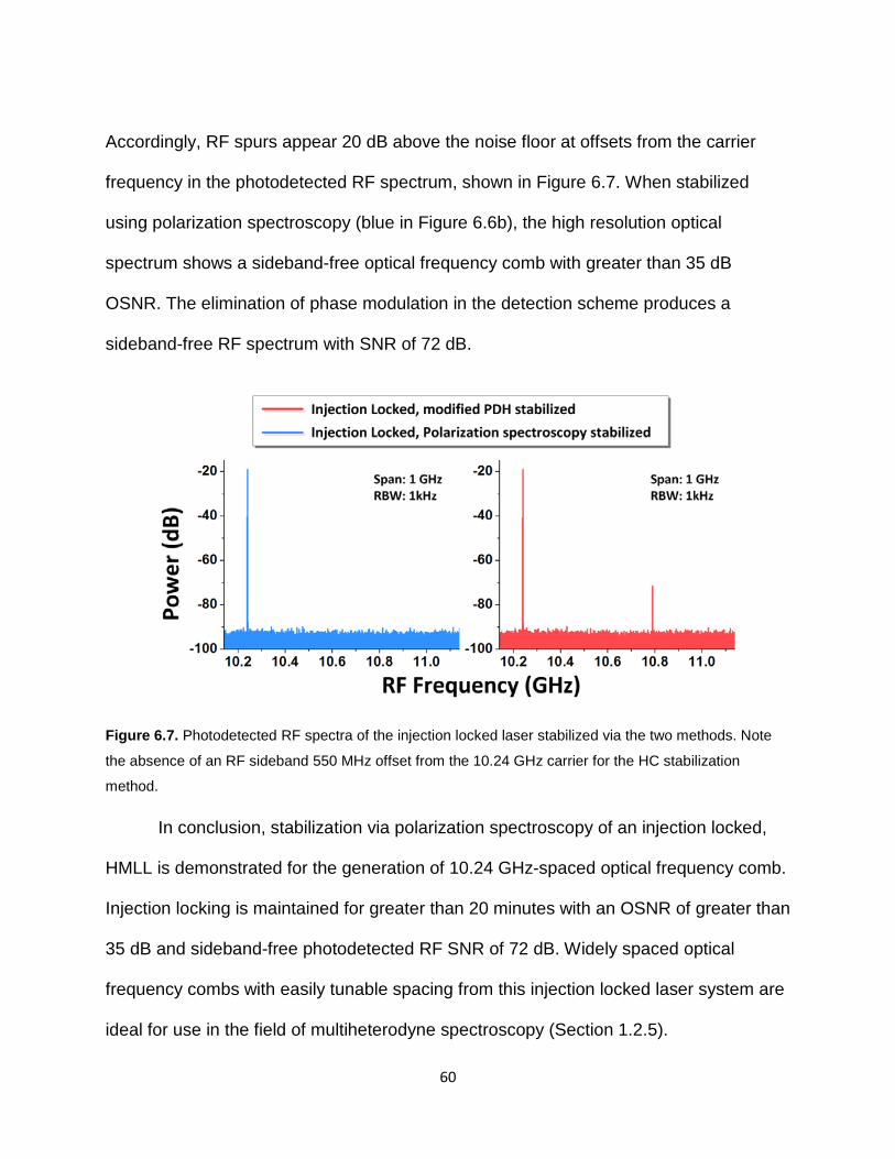
60

Accordingly, RF spurs appear 20 dB above the noise floor at offsets from the carrier

frequency in the photodetected RF spectrum, shown in Figure 6.7. When stabilized

using polarization spectroscopy (blue in Figure 6.6b), the high resolution optical

spectrum shows a sideband-free optical frequency comb with greater than 35 dB

OSNR. The elimination of phase modulation in the detection scheme produces a

sideband-free RF spectrum with SNR of 72 dB.

Figure 6.7. Photodetected RF spectra of the injection locked laser stabilized via the two methods. Note

the absence of an RF sideband 550 MHz offset from the 10.24 GHz carrier for the HC stabilization

method.

In conclusion, stabilization via polarization spectroscopy of an injection locked,

HMLL is demonstrated for the generation of 10.24 GHz-spaced optical frequency comb.

Injection locking is maintained for greater than 20 minutes with an OSNR of greater than

35 dB and sideband-free photodetected RF SNR of 72 dB. Widely spaced optical

frequency combs with easily tunable spacing from this injection locked laser system are

ideal for use in the field of multiheterodyne spectroscopy (Section 1.2.5).

61

CHAPTER 7: CW INJECTION LOCKING OF A COUPLED OPTO-ELECTRONIC OSCILLATOR

Additional features that are desirable in frequency comb sources are low cost

and portability. To that end, the removal of the external RF source used to drive the

laser intensity modulator (IM) is paramount to the creation of a stand-alone optical

frequency comb source. One method to achieve this is regenerative mode-locking. In

this section, a CW injection locked Coupled Opto-Electronic Oscillator (COEO) is

presented with a 10.24 GHz spaced optical frequency comb output as well as a low

noise RF output. A modified Pound-Drever-Hall scheme is employed to ensure long-

term stability of the injection lock. This is achieved by using a fiber stretcher to adjust

the cavity length. The slaved cavity resonance position shifts accordingly to compensate

for cavity resonance drifts relative to the injection seed frequency. High optical signal-to-

noise ratio of ~35 dB is demonstrated with >20 comblines of useable bandwidth. The

optical linewidth, in agreement with injection locking theory, reduces to that of the

injection seed frequency, <5 kHz. Low amplitude and absolute phase noise are

presented from the optical output of the laser system. The integrated pulse-to-pulse

energy fluctuation is found to be reduced by up to a factor of two due to optical injection.

Additional decreases were shown for varying injection powers. This work has been

presented in references [98-101].

Excellent absolute RF phase noise has been reported in the literature using the

COEO configuration [102, 103]. These sources are erbium fiber gain-based,

harmonically mode-locked, and are used primarily for their low-noise RF output and

62

soliton-induced short optical pulses. In contrast, the current work utilizes semiconductor

gain media and offers a stabilized frequency comb output which is useful in the

previously outlined applications (Section 1.2), especially in the burgeoning field of

multiheterodyne detection. This application can often place stringent requirements on

the comb-line spacing of multiple frequency comb sources. While another COEO design

offers a frequency comb output referenced to an intracavity etalon [104], stable

frequency combs with easily tunable comb-line spacing generated using a CW tone are

particularly advantageous for applications such as multiheterodyne detection. This

section features such a source in the form of an optically injection locked COEO. An

extensive characterization of noise properties, including high resolution optical spectra,

RF supermode noise spur suppression, amplitude noise, absolute phase noise, and

Allan deviation, is presented.

7.1 Regenerative Mode-Locking

Without a mode-locking signal applied to the intracavity IM, all laser modes are

free to lase independently, meaning they are do not have a fixed phase relationship.

Upon photodetection, a small RF beating between adjacent cavity modes will be

detected at the cavity fundamental frequency, ν0, as well as 2*ν0, 3*ν0, and so on up to

the bandwidth of the photodetector. One of these small amplitude RF beats could be

selected by an RF filter, amplified, and applied to the intracavity IM to achieve mode-

locking using the laser’s own photodetected output, as shown in the simple schematic in

Figure 7.1. This mechanism is called regenerative mode-locking, and the resulting

system is referred to as a COEO [105].

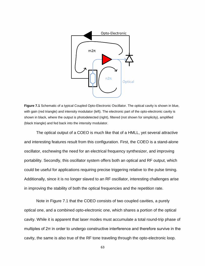
63

Figure 7.1 Schematic of a typical Coupled Opto-Electronic Oscillator. The optical cavity is shown in blue,

with gain (red triangle) and intensity modulator (left). The electronic part of the opto-electronic cavity is

shown in black, where the output is photodetected (right), filtered (not shown for simplicity), amplified

(black triangle) and fed back into the intensity modulator.

The optical output of a COEO is much like that of a HMLL, yet several attractive

and interesting features result from this configuration. First, the COEO is a stand-alone

oscillator, eschewing the need for an electrical frequency synthesizer, and improving

portability. Secondly, this oscillator system offers both an optical and RF output, which

could be useful for applications requiring precise triggering relative to the pulse timing.

Additionally, since it is no longer slaved to an RF oscillator, interesting challenges arise

in improving the stability of both the optical frequencies and the repetition rate.

Note in Figure 7.1 that the COEO consists of two coupled cavities, a purely

optical one, and a combined opto-electronic one, which shares a portion of the optical

cavity. While it is apparent that laser modes must accumulate a total round-trip phase of

multiples of 2π in order to undergo constructive interference and therefore survive in the

cavity, the same is also true of the RF tone traveling through the opto-electronic loop.

64

The particular radio frequency travelling through the opto-electronic loop and used for

mode-locking is ultimately determined by the optical cavity mode spacing. Therefore, in

order to properly achieve mode-locking after an RF tone has been chosen by the optical

cavity, its phase must be adjusted via an RF phase shifter to satisfy the 2π condition

stated above.

7.2 Injection Locked COEO Experimental Setup

Figure 7.2 shows the laser system setup with the feedback loop. Optical gain is

supplied inside the optical cavity via a commercially available semiconductor optical

amplifier (Covega BOA1004) with gain in the 1550 nm spectral region and a saturation

power of 16.5 dBm. Two optical couplers are used to couple light out of the optical

cavity and couple the injection seed into the cavity. A Mach-Zehnder IM is employed to

actively mode-lock via loss modulation. Approximately 1.3 m of dispersion

compensating fiber (D ~ -169 ps/nm∙km) is used to balance the anomalous dispersion of

the ~18 m long optical cavity, comprised primarily of standard single-mode fiber (D ~ 17

ps/nm∙km). This corresponds to a cavity fundamental frequency of ~11 MHz and an

estimated total dispersion of 0.0732 ps/nm for the fiber components of the cavity, not

counting the modulator crystal and the semiconductor gain medium. An optical isolator

is used to ensure unidirectional light propagation in the cavity. The optical cavity is

contained in an insulated enclosure to minimize the effect of environmental factors on

the setup.

The opto-electronic loop components are shown in the top right of Figure 7.2.

Part of the light from the output coupler of the optical cavity is photodetected, and the

65

RF tone at the desired repetition rate of the laser, i.e. 10.24 GHz, is bandpass-filtered,

amplified and applied to the intracavity IM to regeneratively mode-lock the laser. The RF

bandpass filter (16 MHz FWHM) determines the repetition rate of the COEO system,

and can be swapped out for simple and expedient tuning of the comb-line spacing. An

RF phase shifter ensures synchronization of the RF signal with the optical pulses. A low

noise RF output is available by splitting the signal before the IM, an important feature of

the COEO design.

Figure 7.2 Injection Locked COEO system schematic. BPF, Bandpass Filter; DBM, Double Balanced

Mixer; DCF, Dispersion Compensating Fiber; FPS, Fiber Phase Shifter; IC, Injection Coupler; IM, Intensity

Modulator; ISL, Injection Seed Laser; ISO, Isolator; LPF, Lowpass Filter; OC, Output Coupler; PC,

Polarization Controller; PD, Photodetector; PIC, Proportional-Integral Controller; PM, Phase Modulator;

PS, Phase Shifter; RFA, RF Amplifier; SOA, Semiconductor Optical Amplifier.

66

The injection arm consists of a commercially available CW laser at 1550 nm and

a phase modulator (PM) for the Pound-Drever-Hall feedback loop. The CW laser has a

linewidth of <5 kHz and a drift of <300 kHz over 30 s.

The feedback loop for stabilizing a cavity resonance to the stable injection seed

frequency uses an RF frequency of ~500 MHz to drive the PM. The signal on the other

side of the injection port, which has interacted with the optical cavity, is photodetected,

amplified, and mixed in a double balanced RF mixer with the original signal, producing

the sum and difference of the two frequencies. An RF phase shifter is employed in the

reference arm to ensure the two signals are in quadrature. This signal is then lowpass-

filtered to yield a differential error signal, which is used by a servo controller to align a

cavity resonance with the injection seed frequency via an intra-cavity fiber phase shifter.

7.3 Injection Locked COEO Results

7.3.1 Optical, RF Spectra and Time Domain Traces

Figure 7.3 shows optical spectra of the COEO in both the free-running and

injection-locked states. When free-running, the COEO spectrum appears broad and

continuous, spanning the 30 nm shown in Figure 7.3a. Individual comblines are not

resolvable due to the close spacing of resonant laser modes comprising the competing

axial mode groups. The power of each mode is relatively low, and the spectrum is

identical to that of a HMLL. The injection locked spectrum looks markedly different, with

a narrowing of the spectrum to 2.3 nm at -10 dB. Individual optical modes of the COEO

system are also now clearly visible. The selection of a single axial mode group with

locked phase, and the suppression of all other groups are shown by the increase in

67

mode contrast of the 10.24 GHz spaced modes. The suppression of the other

supermodes, coupled with the phase-locking of the 10.24 GHz spaced modes produces

the desired frequency comb output of the laser system. Power per combline in the

resulting frequency comb is higher such that the total average power output of the laser

system is relatively unchanged between the free-running and injection-locked states.

Figure 7.3 (a) Optical spectra of the free-running (black) and injection-locked (red) states. The injection

seed frequency is denoted by a black arrow. (b) High resolution optical spectra (100 MHz resolution). The

optical modes in free-running operation (black) are too closely spaced (11 MHz) for the instrument to

resolve.

The comb expands primarily to the longer wavelength side due to the ability of

the injection seed to deplete gain from the higher energy transitions within the

semiconductor, but not from lower energy transitions. This allows comb generation in

the COEO at wavelengths longer than the injection seed. Optical comb generation is

68

confirmed in Figure 7.3b by measuring the optical spectrum with a high resolution

optical spectrum analyzer. Once again, the free-running (black) trace appears

continuous, since the individual laser modes are not resolvable by the instrument. In the

injection-locked spectrum, 10.24 GHz spaced individual modes are clearly seen. A

suppression of the unwanted axial modes of at least 35 dB is observed from the

selected axial mode group. In separate tests, the optical linewidth of an injection locked

laser system reduces to that of the injection frequency, < 5 kHz.

Figure 7.4a shows the photodetected output of the injection-locked COEO

system. The large tone on the left is the RF carrier frequency near 10.24 GHz. On the

right, the nearest supermode noise spur is seen at an 11 MHz offset, representing the

beating between adjacent optical axial mode groups. The injection-locked spectrum

shows suppression of the spur into the noise floor, >15 dB, corresponding to the

suppression of all axial groups but one. Figure 7.4b details the RF carrier tone in a

smaller span, showing significant RF noise reduction in the wings of the spectrum due

to injection locking. This is due to increased correlation among optical frequencies

contributing to the RF carrier frequency after injection locking. Long-term operation has

been observed for longer than 15 minutes, proving the viability of the feedback

mechanism. Recall that a ~500 MHz frequency is used in the modified Pound-Drever-

Hall scheme for the creation of phase modulation sidebands. Since all three frequencies

are injected into the cavity, the sidebands could inject into other cavity resonances and

appear in the RF signature of the system. This effect is suppressed by careful tuning of

the phase modulation frequency along with the phase in the optoelectronic loop (which

69

strongly affects the repetition rate). The stabilization tone in the photodetected output

was observed to be 54 dB below the carrier, when measured at 500 MHz offset.

Figure 7.4 (a) RF power spectrum of the photodetected COEO optical output, free-running (black) and

injection-locked (red) with fundamental RF tone and one supermode noise spur, suppressed via injection

locking. (b) Zoomed view of fundamental RF tones at ~10.24 GHz.

Figure 7.5 shows the photodetected time domain output of the COEO system in

both the injection locked and free-running cases. Figure 7.5a shows the pulse train with

a ~100 ps period, measured with a photodetector bandwidth of 16 GHz and a sampling

oscilloscope. Note the improved uniformity in pulse amplitude in the injection locked

pulse train (red). This amplitude noise improvement is further quantified below by

extensive amplitude noise analysis.

70

Figure 7.5 Time domain normalized (a) sampling scope and (b) autocorrelation traces of the COEO

output in both free-running (black) and injection-locked (red) cases.

In Figure 7.5b, autocorrelation traces show a 30 ps autocorrelation full-width at

half maximum (FWHM) of pulses directly from the laser system with an average optical

power of ~5 mW. The wings of the injection locked trace appear less noisy. This is due

to the increased correlation of modes in the optical spectrum after suppression of all but

one axial mode group. Pulses directly from the injection locked COEO system are not

transform limited for the optical bandwidth shown, as expected. Semiconductor lasers

do not typically emit transform-limited pulses directly from the laser due to large

nonlinearities in the gain dynamics causing strong linear chirp [92]. Since many of the

intended applications of the system (e.g. optical arbitrary waveform generation,

metrology, multiheterodyne detection) are not concerned with pulsewidth, compression

of the pulse was not explored for the scope of this chapter. However, for applications

where short optical pulses are of particular benefit, pulses from semiconductor lasers

have been shown to be externally compressible to near the transform-limit pulsewidth

[92].

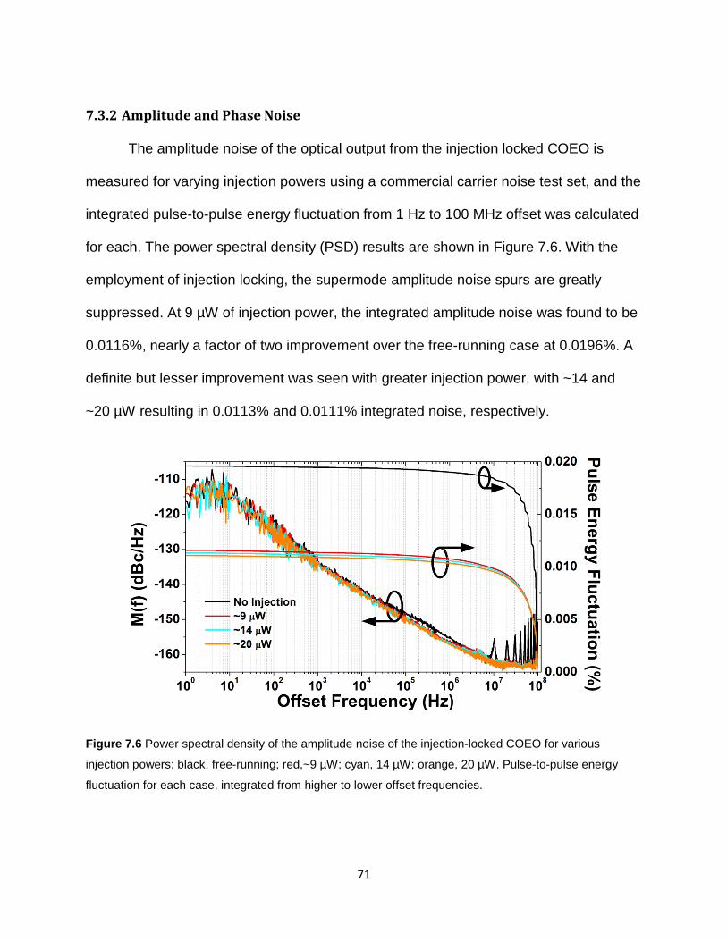
71

7.3.2 Amplitude and Phase Noise

The amplitude noise of the optical output from the injection locked COEO is

measured for varying injection powers using a commercial carrier noise test set, and the

integrated pulse-to-pulse energy fluctuation from 1 Hz to 100 MHz offset was calculated

for each. The power spectral density (PSD) results are shown in Figure 7.6. With the

employment of injection locking, the supermode amplitude noise spurs are greatly

suppressed. At 9 µW of injection power, the integrated amplitude noise was found to be

0.0116%, nearly a factor of two improvement over the free-running case at 0.0196%. A

definite but lesser improvement was seen with greater injection power, with ~14 and

~20 µW resulting in 0.0113% and 0.0111% integrated noise, respectively.

Figure 7.6 Power spectral density of the amplitude noise of the injection-locked COEO for various

injection powers: black, free-running; red,~9 µW; cyan, 14 µW; orange, 20 µW. Pulse-to-pulse energy

fluctuation for each case, integrated from higher to lower offset frequencies.

72

Due to the logarithmic method in which PSD data is plotted, the majority of the

contribution to the reduction in noise comes from the suppression of the supermode

noise in the last (highest frequency) decade. This distribution of noise contribution to the

integrated pulse amplitude fluctuation is also demonstrated by the integration curves

from higher to lower offsets. This measurement was taken with similar optical spectral

bandwidth for all injection-locked cases. Higher injection powers were not tested since

the useable spectral bandwidth decreases with increased injection power.

Applications for RF sources and optical frequency combs benefit from low timing

jitter in the frequency range from the inverse of the measurement time (typically on the

order of 100 Hz) to the Nyquist frequency at half the repetition rate. The COEO output

pulse train resembles that of a HMLL. It should be noted that in HMLLs without a

supermode noise spur suppressing mechanism, the influence of these spurs dominates

the amplitude and phase noise integrated out to fNyquist.

For this reason, phase noise measurements of the COEO system are focused on

observing the suppression of the supermode noise spurs present at multiples of 1/Tcavity,

the fundamental frequency of the cavity. The phase noise of the injection-locked COEO

is measured using the frequency discriminator technique with ~15 μW of injection power

[106]. Since the COEO acts as a stand-alone RF oscillator, the output is compared to its

own delayed signal in order to measure phase noise power spectral density. This

results in an absolute phase noise measurement, which is modulated by the frequency

discriminator envelope due to the relative delay of each RF frequency between the laser

output and its delayed equivalent:

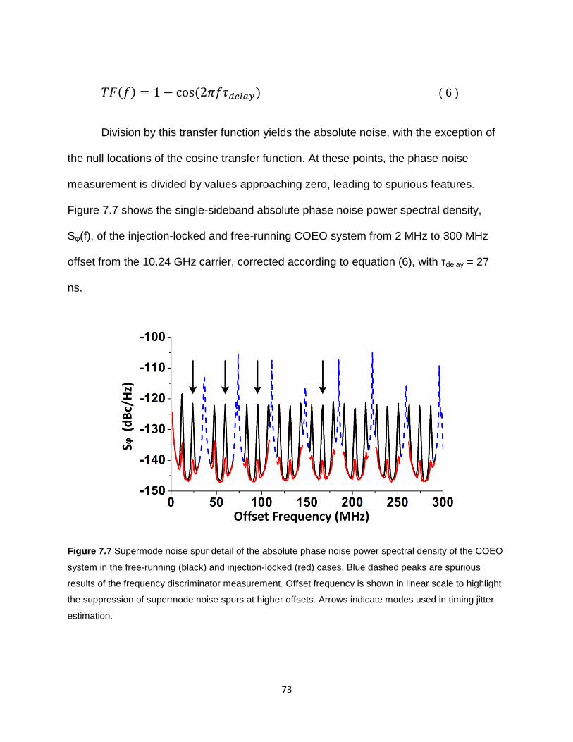
73

𝑇𝐹(𝑓) = 1 − cos (2𝜋𝑓𝜏𝑑𝑒𝑙𝑎𝑦) ( 6 )

Division by this transfer function yields the absolute noise, with the exception of

the null locations of the cosine transfer function. At these points, the phase noise

measurement is divided by values approaching zero, leading to spurious features.

Figure 7.7 shows the single-sideband absolute phase noise power spectral density,

Sφ(f), of the injection-locked and free-running COEO system from 2 MHz to 300 MHz

offset from the 10.24 GHz carrier, corrected according to equation (6), with τdelay = 27

ns.

Figure 7.7 Supermode noise spur detail of the absolute phase noise power spectral density of the COEO

system in the free-running (black) and injection-locked (red) cases. Blue dashed peaks are spurious

results of the frequency discriminator measurement. Offset frequency is shown in linear scale to highlight

the suppression of supermode noise spurs at higher offsets. Arrows indicate modes used in timing jitter

estimation.

74

The figure is deliberately shown in linear frequency scale so as to detail the

supermode noise spur suppression achieved by the injection locking of the system,

found to be ~18 dB by comparing the peak power of the spurs in the free-running case

with their counterparts in the injection-locked case. Noise values significantly affected

by the transfer function are set apart from the rest of the measurement by blue dashed

lines.

Supermode noise spurs in HMLL noise spectra arise from a lack of correlation

between pulses separated by less than the round trip time of the cavity [17]. Multiple

pulses simultaneously traversing the cavity experience different spontaneous emission

influences. The presence of these interleaved, uncorrelated pulse trains leads to

periodicity in the noise spectrum at multiples of 1/Tcavity. This implies that a rough

estimate of the timing jitter integrated to Nyquist can be made via integration/timing jitter

calculation of one period (i.e. one supermode noise spur) and multiplying by √(N/2)

where N is the number of supermode noise spurs present, calculated by N=frep/fcavity.

The timing jitter over a specific range of the single sideband phase noise, L(f), is given

by [93]:

𝜎𝐽 = 𝑇𝑅𝑒𝑝2𝜋

�∫ 𝐿(𝑓)𝑑𝑓𝑓𝑢𝑝𝑝𝑒𝑟𝑓𝑙𝑜𝑤𝑒𝑟

( 7 )

Estimations of the timing jitter were made via this method from four different

peaks within the phase noise spectra, indicated by arrows in Figure 7.7. Where the

‘valleys’ between measurements are made uneven by transfer function influences, a

half integration was performed from the lower valley and multiplied by two. Estimations

75

of the absolute timing jitter integrated to Nyquist for the free-running COEO yielded a

median value of ~420 ± 20 fs. When injection locked, this value dropped significantly to

~115 ± 15 fs. In all cases, timing jitter was suppressed using injection locking by a factor

of at least 3.

Phase noise at low offset frequencies was not measured, but has been shown in

the actively mode-locked case to be greatly influenced by the injection seed. A

reduction in optical linewidth in HMLLs is correlated with a reduction in the ‘knee’

frequency [50]. This strongly influences timing jitter integration, both at low offsets and

in the supermode noise spurs, since the phase noise plot is periodic at 1/Tcavity. Optical

injection locking leads to a reduction in output optical linewidth to that of the injection

seed, and therefore should reduce low-offset phase noise [58]. However, long-term

instabilities in the injection seed frequency will translate to instabilities in the RF output,

as discussed below, and therefore an increase in noise at very low-offset frequencies.

This has also been shown in actively mode-locked injection locked lasers [58, 107].

7.3.3 Allan Deviation

A more common metric for measuring the long-term stability of an RF signal is

the Allan Deviation (ADEV) of an oscillator [108, 109]. An extensive explanation of

ADEV can be found in APPENDIX A. The ADEV of the injection locked COEO was

measured for the photodetected optical output in both free running and injection locked

states for time intervals from 100 ns to 1 s. The results are shown in Figure 7.8. Multiple

frequency measurements are taken at a specific time interval using a Pendulum CNT-

91 frequency counter with zero dead time, and their two-sample variance is calculated.

76

The square root of this is the deviation, yielding each point in the plot. This is then the

degree to which the frequency value in a particular time interval is replicated in the next

measurement of that time interval.

Figure 7.8 Allan Deviation measurements of the Injection Locked COEO from the photodetected optical

output for both injection locked (red triangle) and free-running (black) states.

The traces in the ADEV measurement follow typical trends for measurements of

stand-alone oscillators, decreasing in fractional deviation of the repetition rate to a

certain point, beyond which it begins to increase in value again, a result of long-term

drift [110]. The ADEV of the free-running oscillator reaches a minimum value of 10-9 at

100 ms. The RF (not shown) and optical outputs of the system in each case present

similar values for the ADEV measurement, as expected, since the RF output contains

little difference in carrier frequency from the optical output, apart from amplifier phase

noise and filtering from the RF filter.

77

The injection locked case, however, shows significant divergence at longer time

intervals from the non-injection locked case, reaching a minimum value just below 10-8

at 100 ms – almost a full decade higher than in the free-running case. This is believed

to be due primarily to the instability of the injection seed frequency. In an injection

locked laser with feedback, the cavity length is actively changed to position one

particular resonance at the same frequency as the injection seed. This change in cavity

length invariably changes the position of all other laser resonances and, more

importantly, their spacing. In an actively mode-locked laser, this slight change in

spacing will affect the phase that each optical tone accumulates as it travels around the

cavity, as long as it is still within a resonance to some degree (and therefore doesn’t

experience significant destructive interference). The frequency of the optical tone will

not be affected, as it is built up from the intensity modulator creating sidebands on each

pre-existing optical mode at a frequency spacing determined by the frequency

synthesizer used to mode-lock.

In a regeneratively mode-locked laser, however, this change in cavity length, and

hence in optical mode spacing, is what ultimately determines the repetition rate of the

system as a whole. For example, while a particular RF frequency is fed into the intensity

modulator and the cavity length is tuned to accommodate a perturbation in injection

seed frequency, the optical tones quickly accumulate a different phase than in the

previous steady state. This change in optical phase leads to a different phase and

amplitude (but not yet frequency) of the resulting RF beat at the mode-locking

frequency. As this RF signal travels through the opto-electronic loop, it must also shift

78

frequency slightly in order to maintain a 2π phase shift. In essence, a change in optical

injection frequency leads to a change in the output RF frequency of the injection locked

COEO. Instabilities in the CW laser frequency used to inject therefore lead to higher

ADEV at long time intervals compared to the free-running COEO. The free-running

COEO will experience the same effect due to normal cavity drift, but at longer time

scales than that of a COEO slaved to a drifting CW laser frequency. This result could be

improved by improving the long-term stability of the injection seed frequency.

7.4 RF Frequency dependence on Injected Optical Frequency of Injection Locked COEO

For various applications of mode-locked laser sources and frequency combs,

stability of the comb spacing, and hence the RF tone produced by photodetection, is of

particular importance. In a COEO, the stability of this tone is greatly influenced by the

optical cavity length as well as the phase drift (also a cavity length change) in the opto-

electronic loop. In previous experiments (Section 7.3.3), the stability of the injection

frequency has also been shown to influence the RF stability of the COEO output. This

section explores this relationship in greater detail and has been presented at the IEEE

Photonics Conference in 2011 [111].

A schematic of the injection locked COEO used is shown in Figure 7.9a and is

much the same as that shown in Figure 7.2. The optical cavity is shown in blue, while

RF links are shown in black and the injection arm is shown in red. The CW lasers used

to injection lock (Orbits Lightwave ETH-1550; Koheras BME 15ThAI) are commercially

79

available and operating at 1550 nm and 1540 nm, respectively, with <10 kHz optical

linewidth.

Figure 7.9 (a) Schematic of the injection locked COEO with feedback stabilization. (b) Experimental setup

for measurement of optical-to-RF instability transfer.

As a stand-alone RF oscillator, the RF stability of the injection locked COEO is

important for RF photonic applications where long-term stable operation is necessary,

such as coherent communications and remote sensing. However, the Allan Deviation

(ADEV) [108] of the injection locked COEO was found to increase compared to the free-

running case for measurement times greater than 1 ms [100]. This experiment seeks to

investigate this phenomenon by comparison to ADEV measurements of the CW

injection laser when beat against a stable frequency reference (Menlo FC-1550). In

addition, the RF output from the injection locked COEO was observed relative to the

optical frequency shift of the injection seed laser.

80

7.4.1 Experimental Results

ADEV measurements were taken of the 10.25 GHz1 RF output of the free-

running COEO (without optical injection) and when injection locked with two different

CW lasers with different ADEV signatures. Additionally, the ADEV of heterodyne beat

tones between the CW injection seed lasers and the reference frequency comb were

also measured. All measurements were normalized to their respective nominal ADEV

measurement frequencies (~10.25 GHz for RF, 1.93E14 Hz for Orbits, 1.9478E14 Hz

for Koheras) and are plotted in Figure 7.10a. For measurement times up to 1 ms, the

COEO in both the free-running and injection locked states demonstrate the same

stability. However, in both injection locked cases, the ADEV increased for measurement

times greater than 1 ms, mimicking the shape of the respective injection laser’s ADEV

measurement, as shown in Figure 7.10a. This is believed to be due to the instabilities of

the injection seed frequency transferring into RF frequency instability.

1 Due to the nature of the COEO system and the configuration of this particular optical cavity, the repetition rate for the RF instability transfer experiments was 10.25 GHz. Repeatability at other repetition rates is assumed based on empirical evidence.

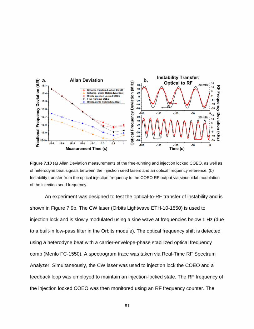
81

Figure 7.10 (a) Allan Deviation measurements of the free-running and injection locked COEO, as well as

of heterodyne beat signals between the injection seed lasers and an optical frequency reference. (b)

Instability transfer from the optical injection frequency to the COEO RF output via sinusoidal modulation

of the injection seed frequency.

An experiment was designed to test the optical-to-RF transfer of instability and is

shown in Figure 7.9b. The CW laser (Orbits Lightwave ETH-10-1550) is used to

injection lock and is slowly modulated using a sine wave at frequencies below 1 Hz (due

to a built-in low-pass filter in the Orbits module). The optical frequency shift is detected

using a heterodyne beat with a carrier-envelope-phase stabilized optical frequency

comb (Menlo FC-1550). A spectrogram trace was taken via Real-Time RF Spectrum

Analyzer. Simultaneously, the CW laser was used to injection lock the COEO and a

feedback loop was employed to maintain an injection-locked state. The RF frequency of

the injection locked COEO was then monitored using an RF frequency counter. The

82

results are shown in Figure 7.10b, where a clear transfer of instability from the injection

optical frequency to the output RF frequency of the injection locked COEO is

demonstrated. Various modulation rates and amplitudes of the optical frequency were

measured yielding values of the ratio of optical-to-RF frequency change between 4800

and 8700 Hz/Hz.

7.4.2 Discussion and Conclusion

With the modified PDH stabilization utilized in the injection locked COEO, the

laser cavity is adjusted such that the slaved cavity resonance follows the injection seed

frequency. Since the exact RF frequency at the appropriate mode-locking harmonic is

determined from the laser cavity itself in a regeneratively mode-locked system, changes

in cavity length result in changes in repetition rate and hence output RF frequency from

the COEO. Therefore, instabilities in the injected optical frequency will cause

degradation in the long-term stability of the injection locked COEO as an RF oscillator.

This has been demonstrated by a change in ADEV of the injection locked COEO for

measurement times longer than 1 ms—both relative to a free-running COEO and when

slaved to two different injection lasers with unique ADEV curves. Direct transfer of the

optical injection frequency instability to the output RF frequency is also demonstrated

via frequency counter measurements while the injection seed frequency is modulated.

Further investigation of the origins of this RF instability will lead to better injection locked

stand-alone oscillators providing both low-noise RF and high quality optical frequency

comb outputs for photonic applications.

83

CHAPTER 8: CONCLUSION

Stabilized, high repetition rate, semiconductor-based mode-locked lasers and

frequency comb sources have a variety of potential uses in coherent communications,

signal processing, optical clocking, and frequency metrology. Low noise operation is

necessary for these applications, and the potential of a source sans any external

microwave reference is appealing. In particular, the generation of widely tunable

frequency combs with these qualities would be advantageous in various applications

and measurements such as multiheterodyne spectroscopy. Single frequency injection

locking of harmonically mode-locked semiconductor lasers is demonstrated to be

effective in reduction of phase and amplitude noise and suppression of unwanted

optical supermode groups so as to create an optical frequency comb with wide (GHz)

comb spacing. Due to the harmonic nature of the mode-locking mechanism, the

frequency comb spacing is also widely tunable. Long-term stabilization of this injection

locked state can be achieved by either Pound-Drever-Hall frequency locking or

polarization spectroscopy of the active laser cavity. Simulation and analysis of both

error signal techniques as applied to active cavities with semiconductor gain is

presented, incorporating amplification through gain and an arcsin phase profile adjusted

as per the linewidth enhancement factor. Suppression of unwanted optical modes of 36

dB and supermode noise spur suppression of 14 dB is achieved. Injection locking of a

regeneratively mode-locked system is demonstrated, obviating the need for a frequency

synthesizer, and resulting in a stand-alone frequency comb source. Extensive

characterization of the stand-alone frequency comb source is also presented.

84

APPENDIX A: ALLAN DEVIATION MEASUREMENT

85

A widely accepted measurement of the stability of an oscillator about a particular

frequency is the Allan Deviation (ADEV) [108, 109]. The square of this is also

sometimes used, and is referred to as the Allan Variance. ADEV is calculated using

various time scales, as will be discussed later, and is normalized to a nominal frequency

and presented as a spectrum of fractional unit values along an axis of measurement

times. This appendix will serve to explain how ADEV is calculated, its usefulness in

measuring oscillator stability relative to the well-known standard deviation, as well as

how it is experimentally measured. In addition to the two seminal references included

above and in the text of section 7.3.3, references [112-115] are extremely useful in

gaining a greater understanding of the concept and were used in part to compile this

appendix. Allan [116] and Rubiola [110] have also outlined the specific conversion

relationships between laser phase noise and ADEV measurements.

Mathematical Deviations are useful in analysis of data to quantify and represent,

within a particular dataset, variations from a standard value in a way that is easily

comparable to other datasets from separate measurements. The well-known Standard

Deviation (STDEV) compares values within a dataset to the mean of the same dataset,

as shown by the STDEV equation given in Eq. ( 8 ). It should be noted that the dataset

values are resulting from independent trials with ostensibly the same conditions, and the

resulting STDEV is a single representative value. If the spread of values within the

dataset is quite large, then the value of the STDEV will be high, and the converse is true

if all values within the set are within a narrow range about the mean. This type of

deviation is quite useful for distilling the characteristic variation down to a single value

86

which can be compared to the next dataset when the variation of values follows a

“Normal Distribution” about the mean, which arises in many situations described above,

where independent trials with the same conditions exist. When the dataset is a

representative sample of a larger population, it is often used to infer the distribution of

the larger population as well.

𝜎 = �1𝑁∑[𝑥𝑘 − �̅�]2 ( 8 )

A unique challenge is presented when applying a deviation to a set of values that

are not independently determined from similar circumstances, such as a set of scores

on a test, but are derived from the previous value with some additional influences, like

the cumulative distance traveled in a car at any given point in time. The car’s position

from the origin at the end of hour x depends greatly on its position at the end of hour x-

1, as well as its average speed over that hour. Such is the case in the wandering

frequency emitted from an oscillator. Many sources of noise affect the frequency of the

signal, on a variety of timescales. In other words, there are slow and fast fluctuations of

the instantaneous frequency. Given these many timescales, calculating a single

representative value based purely on the ‘mean’ value of the signal is not only

meaningless, but nonsensical, as the value of the mean will continue to change with

measurement time.

87

Figure A.1 Simulated instantaneous frequency values of a non-stable signal at a starting frequency of 10

GHz.

Consider the signal in Figure A.1, where the instantaneous frequency is

fluctuating randomly on a very short time scale, but is also slowly wandering with larger

amplitude. Any STDEV calculated from a subset of values must be representative of the

whole ‘population,’ but calculating based on the first 200 values would not account for

the large variation from that mean happening in values after that. Using a larger

‘representative’ dataset would result in large deviations, considering at a glance how

many values are far away from the middle or ‘nominal’ frequency, as well as gloss over

the small amplitude fluctuations happening on small time scales. Therefore, a deviation

that is useful in describing such contiguous wandering in a value with variations on

many time scales must differ from the STDEV in at least two ways: 1) it must be a

spectrum, representative of the many time scales on which variations can happen and

2) it must not be based upon a ‘global’ mean or average, since this average could be

vastly different for each subset of values attempting to represent the global

88

characteristics, which would greatly affect the measurement. ADEV measurements are

designed to accomplish both of these by taking many averages over the same time

period, resulting in a single statistical deviation for that time period. The measurement

and calculation is then repeated for other measurement time periods, with each

deviation being plotted along the measurement time axis, as shown in the ADEV

example graph in Figure A.2. The resulting curve is representative of the frequency

stability of the oscillator under test.

Figure A.2 Typical Allan Deviation plot showing calculated fractional deviation values for increasing

measurement times.

Equation and its Explanation

The equation for ADEV (σy) is given by Eq. ( 9 ), and differs from the Allan

Variance (AVAR) only by the square root. The differences between averages is taken

for the entire dataset, then individually squared and an expectation value is calculated

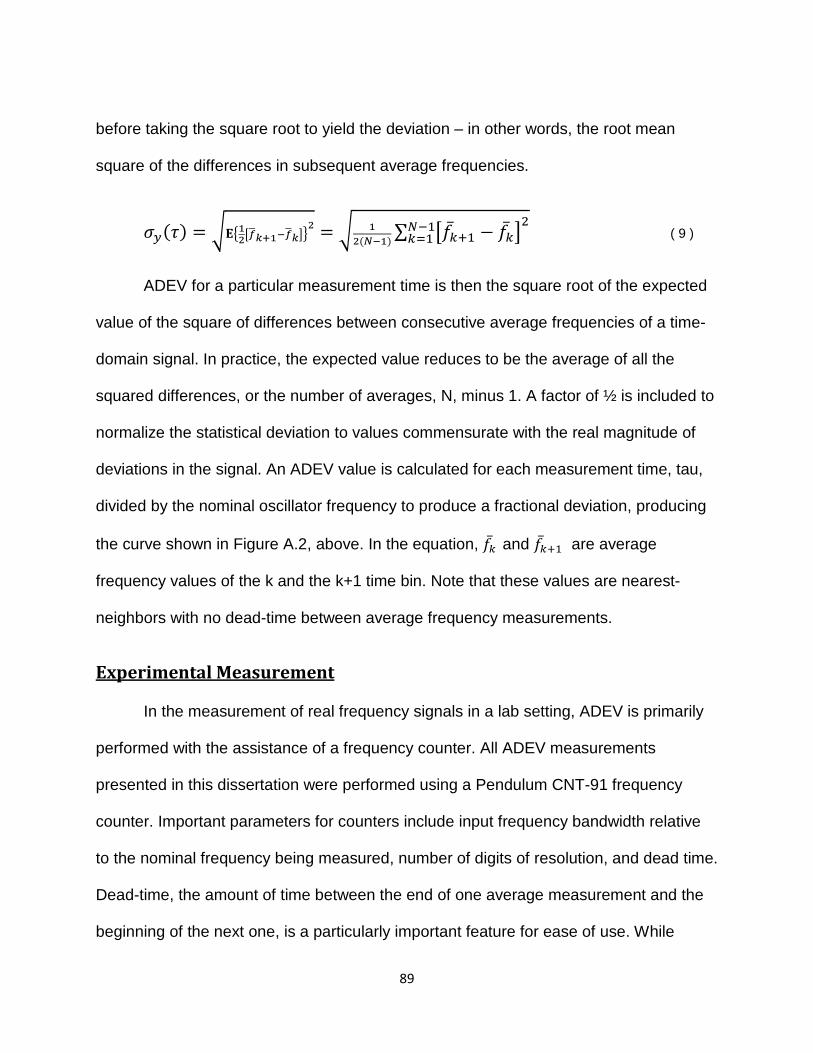
89

before taking the square root to yield the deviation – in other words, the root mean

square of the differences in subsequent average frequencies.

𝜎𝑦(𝜏) = �𝐄�12�𝑓�𝑘+1−𝑓�𝑘��2 = � 1

2(𝑁−1)∑ �𝑓�̅�+1 − 𝑓�̅��

2𝑁−1𝑘=1 ( 9 )

ADEV for a particular measurement time is then the square root of the expected

value of the square of differences between consecutive average frequencies of a time-

domain signal. In practice, the expected value reduces to be the average of all the

squared differences, or the number of averages, N, minus 1. A factor of ½ is included to

normalize the statistical deviation to values commensurate with the real magnitude of

deviations in the signal. An ADEV value is calculated for each measurement time, tau,

divided by the nominal oscillator frequency to produce a fractional deviation, producing

the curve shown in Figure A.2, above. In the equation, 𝑓�̅� and 𝑓�̅�+1 are average

frequency values of the k and the k+1 time bin. Note that these values are nearest-

neighbors with no dead-time between average frequency measurements.

Experimental Measurement

In the measurement of real frequency signals in a lab setting, ADEV is primarily

performed with the assistance of a frequency counter. All ADEV measurements

presented in this dissertation were performed using a Pendulum CNT-91 frequency

counter. Important parameters for counters include input frequency bandwidth relative

to the nominal frequency being measured, number of digits of resolution, and dead time.

Dead-time, the amount of time between the end of one average measurement and the

beginning of the next one, is a particularly important feature for ease of use. While

90

correction factors do exist for non-zero dead time while performing ADEV

measurements, a zero dead-time frequency counter (such as the one used) makes this

additional calculation unnecessary. In addition, a reference clock is necessary, either

internal or from an external input. In either mode, reasonable confidence should exist

that the reference clock is of better or similar stability as the oscillator under test. To this

end, for state of the art ADEV measurements demonstrating record low instability, two

identical oscillator systems are often compared against one another.

The frequency counter works by counting the number of zero crossings of the

oscillating electrical signal for a particular time interval based on the reference clock.

Many features exist in frequency counters to condition a noisy signal for proper

measurement, and each counter’s manual should be consulted for these features. Only

the basics will be addressed here for the sake of understanding the process.

Figure A.3 a) Oscillating signal of interest in blue with zero crossings shown by black dots. Boxes shown

represent average frequency measurement times of b) 100 ns, c) 1 μs, d) 10 μs, and e) 100 μs.

Figure A.3 illustrates an oscillating voltage signal (blue). As implied above, the

counter is able to detect when the voltage passes between positive and negative (zero

crossings, shown as black dots on the blue signal), and uses the number of these

91

crossings to determine the average frequency within a particular time interval. This is

shown in Figure A.3b by the black boxes, each being its own frequency average

measurement. Note that the boxes are contiguous, signifying the lack of dead-time

between frequency measurements. Once ADEV is calculated for a particular timescale,

e.g. 100 ns, another set of frequency averages are measured using progressively larger

averaging times (Figure A.3c –Figure A.3e). The resulting ADEV values form the

representative curve, an example of which is shown in Figure A.2.

Simulation

To illustrate the measurement, a simulation was designed to perform an ADEV

calculation on a set of instantaneous frequency values with a nominal frequency on the

same order of that of interest in our ADEV experiments – 10 GHz. The simulation was

performed in Matlab, and the code is included in APPENDIX C. The instantaneous

frequency dataset is generated by starting at the nominal frequency and adding a

cumulative sum of two types of noise of interest to us: white noise (WN) and random

walk (RW). Each value, therefore, is produced from the previous value plus an amount

of each type of noise. The noise magnitudes can be specified and are defined in the

frequency domain and relative to f0, the nominal frequency.

The instantaneous values, shown in Figure A.1, above, are defined on an

arbitrary timescale, such that, while they can be considered ‘instantaneous’ in a broad

descriptive sense, they can also be used as frequency averages of the signal on the

smallest measurement time in the ADEV spectrum of values. Therefore, all other

measurement times are specified in terms of this smallest time, tau. With this first set of

92

‘averages,’ the ADEV calculation is performed for measurement time tau and divided by

f0. Averages of these values are then taken with measurement times of 2𝑀 ∗ 𝑡𝑎𝑢, and

the ADEV calculation performed. Figure A.4- Figure A.8, below, illustrate this averaging.

Figure A.4 Instantaneous frequency values (blue) and averages (black) over four instantaneous time

increments.

Figure A.5 Instantaneous frequency values (blue) and averages (light blue) over 16 instantaneous time

increments.

93

Figure A.6 Instantaneous frequency values (blue) and averages (green) over 64 instantaneous time

increments.

Figure A.7 Instantaneous frequency values (blue) and averages (blue straight lines) over 256

instantaneous time increments.

94

Figure A.8 Instantaneous frequency values (top, blue) and averages over several instantaneous time

increments.

Examples and Explanations

A similar set of values (arrived at with the same amount of WN and RW) and its

associated ADEV curve are shown in Figure A.9a and Figure A.9b. Note that the ADEV

reaches a minimum value at 2*tau and begins to rise in instability for greater

measurement times due to the small effect of white noise on the signal and the large,

visible effect of random walk. Figure A.9c shows an associated variation on the STDEV

of the signal, substituting the local average for the global average, an admittedly flawed

method allowing for a deviation similar to that of STDEV to be calculated over a series

of measurement times. Note that the value of STDEV remains a relatively constant

value, obscuring any information on variations happening at different timescales. The

difference between the ADEV and associated modified STDEV is shown (green curve)

for clarity. A second example with similar parameters is shown in Figure A.10.

95

Figure A.9 a) Instantaneous frequency values starting at 10 GHz and calculated with equal parts white

noise and random walk. b) ADEV curve of the frequency values. c) Modified STDEV curve (blue) and

difference between ADEV and STDEV (green) illustrating a lack of information given by such a

measurement.

96

Figure A.10 a) A second example of instantaneous frequency values starting at 10 GHz and calculated

with equal parts white noise and random walk. b) ADEV curve of the frequency values. c) Modified

STDEV curve (blue) and difference between ADEV and STDEV (green).

97

Figure A.11a-c show another example of a set of instantaneous frequency values

defined with a half order of magnitude more white noise, along with the corresponding

ADEV and STDEV curves. Note that the inclusion of more white noise prevents the

ADEV from converging and reaching minimum instability until the 8*tau measurement

time, while the STDEV is still a constant value.

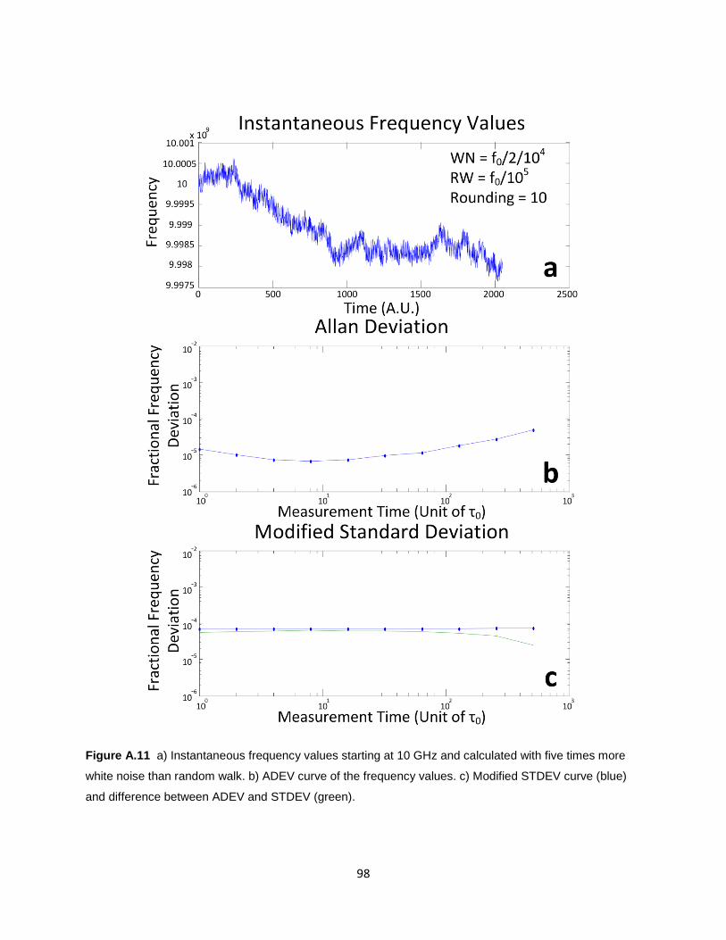
98

Figure A.11 a) Instantaneous frequency values starting at 10 GHz and calculated with five times more

white noise than random walk. b) ADEV curve of the frequency values. c) Modified STDEV curve (blue)

and difference between ADEV and STDEV (green).

99

Figure A.12a and b and Figure A.13a and b illustrate an intriguing yet very small

limitation of the ADEV measurement method. In the definition of the instantaneous

frequency values, a sinusoidal modulation is included with a magnitude on the same

order as that of the white noise. The ADEV curve is significantly affected by this

modulation, as seen in Figure A.12b and Figure A.13b by the existence of a bump for

short timescales followed by a sharp dip in the curve.

100

Figure A.12 a) Instantaneous frequency values starting at 10 GHz and calculated with five times more

white noise than random walk, as well as a rounding error and sinusoidal modulation introduced onto the

signal. b) ADEV curve of the frequency values. Note the effect of the modulation on the curve shape at

8*τ0. c) Modified STDEV curve (blue) and difference between ADEV and STDEV (green).

101

5

Figure A.13 a) A second example of instantaneous frequency values starting at 10 GHz and calculated

with five times more white noise than random walk, as well as a rounding error and sinusoidal modulation

introduced onto the signal. b) ADEV curve of the frequency values. Note that the modulation is at a

quarter of the frequency of the previous figure, and the associated anomaly in the ADEV curve is at 32*τ0,

four times that of the previous example. c) Modified STDEV curve (blue) and difference between ADEV

and STDEV (green).

102

The reasoning for this is illustrated by Figure A.14, where an instantaneous

frequency dataset which has been modulated with a low frequency sin wave and the

corresponding ADEV averages are shown. The averages have been offset in the

vertical direction for easier visualization. For timescales much shorter than the period of

the sin modulation (green, red, and black at the top), nearest neighbor averages are

quite different from each other, resulting in an increase in instability similar to the effect

of random walk. As the averaging time begins to approach half the period of the

modulation (teal, yellow, and green in the middle), the large fluctuations due to the

modulation begin to be washed out and differences between nearest neighbor averages

are much lower, leading to an abrupt reduction in the calculated ADEV instability

(occurring at 32*tau in the example in Figure A.13). At larger timescales than this, the

modulation is, for the most part, averaged out and the residual instability of the oscillator

begins to dominate the ADEV measurement curve. This effect can happen in real

oscillator ADEV measurements and should be watched out for.

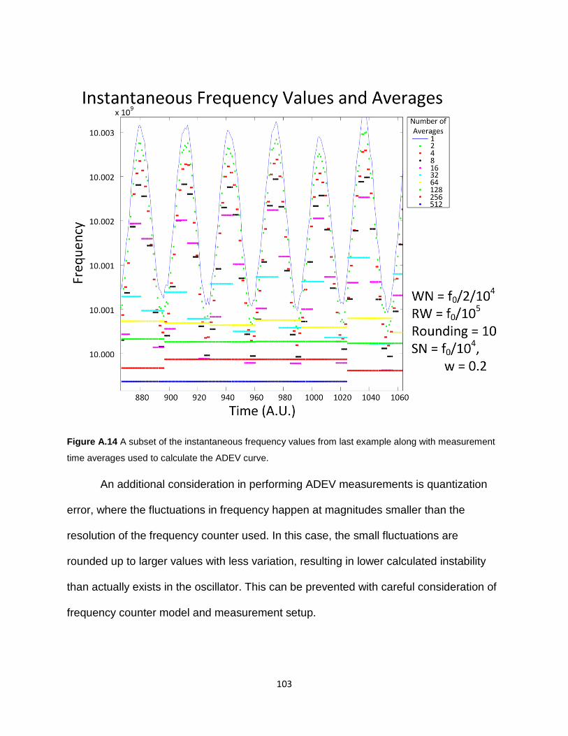
103

Figure A.14 A subset of the instantaneous frequency values from last example along with measurement

time averages used to calculate the ADEV curve.

An additional consideration in performing ADEV measurements is quantization

error, where the fluctuations in frequency happen at magnitudes smaller than the

resolution of the frequency counter used. In this case, the small fluctuations are

rounded up to larger values with less variation, resulting in lower calculated instability

than actually exists in the oscillator. This can be prevented with careful consideration of

frequency counter model and measurement setup.

104

APPENDIX B: LIST OF PUBLICATIONS AND CONFERENCES

105

Primary Author

C. G. Williams, F. Quinlan, and P. J. Delfyett Jr., "Injection Locked Mode-Locked Laser with Long-Term

Feedback Stabilization," in Conference on Lasers and Electro-Optics/Quantum Electronics and Laser

Science Conference and Photonic Applications Systems Technologies, 2008, p. CThP5.

C. Williams and P. J. Delfyett, "CW Injection Locking of Oscillators for Long-Term Stability of Frequency

Combs," presented at the International OSA Network of Students (IONS) - North America, College Park,

MD, 2009.

C. Williams, F. Quinlan, J. Davila-Rodriguez, and P. J. Delfyett Jr., "Optical Injection Locking of a Coupled

Opto-Electronic Oscillator," in Conference on Lasers and Electro-Optics/International Quantum

Electronics Conference and Photonic Applications Systems Technologies, 2009, p. CThF3.

C. Williams, F. Quinlan, J. Davila-Rodriguez, D. Mandridis, and P. J. Delfyett, "Injection Locked Coupled

Optoelectronic Oscillator with Long-Term Feedback Stabilization," in Frontiers in Optics, 2009, p. FMD2.

C. Williams, F. Quinlan, and P. J. Delfyett, "CW injection locking for long-term stability of frequency

combs," in Enabling Photonics Technologies for Defense, Security, and Aerospace Applications V,

Orlando, FL, USA, 2009, pp. 733903-10.

C. Williams, F. Quinlan, and P. J. Delfyett, "Injection Locked Mode-Locked Laser with Long-Term

Feedback Stabilization," presented at the International OSA Network of Students (IONS) - 5 Barcelona,

Sp, 2009.

C. Williams, F. Quinlan, and P. J. Delfyett, "Injection-Locked Mode-Locked Laser With Long-Term

Stabilization and High Power-per-Combline," IEEE Photonics Technology Letters, vol. 21, pp. 94-96, Jan-

Feb 2009.

C. Williams, D. Mandridis, J. Davila-Rodriguez, and P. J. Delfyett, "Injection locked coupled opto-

electronic oscillator for optical frequency comb generation," in SPIE Defense, Security, and Sensing,

Orlando, FL, 2011.

C. Williams, J. Davila-Rodriguez, D. Mandridis, and P. J. Delfyett, "Noise Characterization of an Injection-

Locked COEO With Long-Term Stabilization," Lightwave Technology, Journal of, vol. 29, pp. 2906-2912,

2011.

C. Williams, D. Mandridis, J. Davila-Rodriguez, A. Klee, and P. J. Delfyett, "Dependence of RF frequency

on injected optical frequency of an injection locked coupled opto-electronic oscillator," in Photonics

Conference (PHO), 2011 IEEE, 2011, pp. 477-478.

106

C. Williams, J. Davila-Rodriguez, K. Bagnell, and P. J. Delfyett Jr., "Stabilization of an Injection Locked

Harmonically Mode-Locked Laser via Polarization Spectroscopy for Frequency Comb Generation," in

Lasers and Electro-Optics (CLEO), 2012 Conference on, San Jose, CA, 2012, p. JTh2A.50

C. Williams, J. Davila-Rodriguez, K. Bagnell, and P. J. Delfyett, "Tunable frequency combs for photonic

applications," in Avionics, Fiber- Optics and Photonics Technology Conference (AVFOP), 2012 IEEE,

2012, pp. 7-8.

Secondary Author

F. Quinlan, C. Williams, S. Ozharar, and P. J. Delfyett, "Measurement of the comb dynamics for feedback

control of an etalon-based coupled optoelectronic oscillator," Optics Letters, vol. 33, pp. 1422-1424, Jul 1

2008.

F. Quinlan, C. Williams, S. Ozharar, and P. J. Delfyett, "Fixed-point frequency measurements of an

intracavity etalon-based coupled optoelectronic oscillator," in IEEE Lasers and Electro-Optics Society,

2008. LEOS 2008. 21st Annual Meeting of the, 2008, pp. 628-629.

F. J. Quinlan, C. Williams, S. Ozharar, and P. J. Delfyett, "Self-Stabilization of the Optical Frequencies

and Pulse Repetition Rate in a Coupled Optoelectronic Oscillator," in Conference on Lasers and Electro-

Optics/Quantum Electronics and Laser Science Conference and Photonic Applications Systems

Technologies, 2008, p. CTuM3.

F. Quinlan, C. Williams, S. Ozharar, S. Gee, and P. J. Delfyett, "Self-Stabilization of the Optical

Frequencies and the Pulse Repetition Rate in a Coupled Optoelectronic Oscillator," Journal of Lightwave

Technology, vol. 26, pp. 2571-2577, Jul-Aug 2008.

J. Davila-Rodriguez, M. Akbulut, C. Williams, and P. J. Delfyett, "Multi-heterodyne mixing of frequency

stabilized combs for ultrafast signal processing," in SPIE Defense, Security, and Sensing, 2010.

J. Davila-Rodriguez, I. Ozdur, C. Williams, and P. J. Delfyett, "A Frequency Stabilized Semiconductor

Mode-Locked Laser with a Phase Modulator and an Intra-Cavity Etalon," in Lasers and Electro-Optics

(CLEO) and Quantum Electronics and Laser Science Conference (QELS), 2010 Conference on, 2010, p.

CWJ5.

J. Davila-Rodriguez, I. Ozdur, C. Williams, and P. J. Delfyett, "A semiconductor-based, frequency-

stabilized mode-locked laser using a phase modulator and an intracavity etalon," Opt. Lett., vol. 35, pp.

4130-4132, 2010.

J. Davila-Rodriguez, C. Williams, M. Akbulut, and P. J. Delfyett, "Multi-heterodyne characterization of

multi-gigahertz spaced optical frequency comb sources," in Lasers and Electro-Optics (CLEO) and

Quantum Electronics and Laser Science Conference (QELS), 2010 Conference on, 2010, pp. 1-2.

107

D. Mandridis, I. Ozdur, C. Williams, and P. J. Delfyett, "100 MHz chirped pulse and frequency comb laser

source using an intra-cavity etalon and long-term stabilization," in IEEE Photonics Society, 2010 23rd

Annual Meeting of the, 2010, pp. 301-302.

M. Bagnell, J. Davila-Rodriguez, C. Williams, and P. J. Delfyett, "White light sampling and cross-

correlation via multi-heterodyne detection with an optical frequency comb," in Lasers and Electro-Optics

(CLEO), 2011 Conference on, 2011, pp. 1-2.

J. Davila-Rodriguez, M. Bagnell, C. Williams, and P. J. Delfyett, "Multiheterodyne Detection for Spectral

Compression and Downconversion of Arbitrary Periodic Optical Signals," Lightwave Technology, Journal

of, vol. 29, pp. 3091-3098, 2011.

J. Davila-Rodriguez, I. Ozdur, C. Williams, D. Mandridis, P. J. Delfyett, J. J. Plant, and P. W. Juodawlkis,

"Ultralow noise, etalon stabilized, 10 GHz optical frequency comb based on a Slab-Coupled Waveguide

Amplifier," in Lasers and Electro-Optics (CLEO), 2011 Conference on, 2011, pp. 1-2.

J. Davila-Rodriguez, C. Williams, M. Bagnell, and P. J. Delfyett, "Frequency combs with multi-gigahertz

spacing from semiconductor mode-locked lasers and applications in multiheterodyne detection for the

measurement of arbitrary optical waveforms," in International Summer Session: Lasers and Their

Applications, Changchun, China, 2011, p. Tu11.

P. J. Delfyett, D. Mandridis, C. Williams, I. Ozdur, M. Bagnell, and A. Klee. (2011, 23 March 2011). Diode

laser produces low-noise chirped pulses. SPIE Newsroom. Available: http://spie.org/x47376.xml

D. Mandridis, C. Williams, I. Ozdur, and P. J. Delfyett, "Low noise stabilized chirped pulse Theta laser for

photonic ADC," in Lasers and Electro-Optics (CLEO), 2011 Conference on, 2011, pp. 1-2.

D. Mandridis, C. Williams, I. Ozdur, and P. J. Delfyett, "Low noise chirped pulse mode-locked laser using

an intra-cavity Fabry-Pérot etalon," Opt. Express, vol. 19, pp. 8994-8999, 2011.

D. Mandridis, C. Williams, I. Ozdur, A. Klee, and P. J. Delfyett, "Semiconductor-based low-noise 100 MHz

chirped pulse laser source based on a theta cavity design with an intra-cavity etalon and long-term

stabilization (Invited)," in SPIE Defense, Security, and Sensing, Orlando, FL, 2011.

A. Klee, D. Mandridis, C. Williams, and P. J. Delfyett, "Direct Comparison of Semiconductor and Erbium-

Based Frequency Stabilized Harmonically Mode-Locked Lasers," in IEEE Photonics Conference, 2011,

Arlington, VA, 2011, pp. 887-888.

J. Davila-Rodriguez, M. Bagnell, C. Williams, P. J. Delfyett, J. J. Plant, and P. W. Juodawlkis, "An all-

diode ultralow noise 10 GHz frequency comb and MOPA system with 0.39 W output power based on

Slab-Coupled Optical Waveguide Amplifiers," in Lasers and Electro-Optics (CLEO), 2012 Conference on,

2012, pp. 1-2.

http://spie.org/x47376.xml

108

M. D. Weed, C. Williams, P. J. Delfyett, and W. V. Schoenfeld, "Feedback in coupled-resonance optical

waveguides," in Lasers and Electro-Optics (CLEO), 2012 Conference on, 2012, pp. 1-2.

P. J. Delfyett, M. Bagnell, S. Bhooplapur, J. Davila-Rodriguez, N. Hoghooghi, I. Ozdur, M. Piracha, and C.

Williams, "Coherent optical signal processing using optical frequency combs," in Avionics, Fiber- Optics

and Photonics Technology Conference (AVFOP), 2012 IEEE, 2012, pp. 22-23.

J. Davila-Rodriguez, C. Williams, P. J. Delfyett, J. J. Plant, and P. W. Juodawlkis, "All-diode generation

and amplification of 10 GHz pulse-trains from coupled-cavity mode-locked lasers using Slab-Coupled

Waveguide Amplifiers," in Avionics, Fiber- Optics and Photonics Technology Conference (AVFOP), 2012

IEEE, 2012, pp. 70-71.

A. C. Klee, J. Davila-Rodriguez, M. Bagnell, and P. J. Delfyett, "Multiheterodyne detection for self-

referenced characterization of complex arbitrary waveforms from largely detuned optical frequency

combs," in Avionics, Fiber- Optics and Photonics Technology Conference (AVFOP), 2012 IEEE, 2012,

pp. 102-103.

A. Klee, J. Davila-Rodriguez, M. Bagnell, and P. J. Delfyett, "Self-referenced spectral phase retrieval of

dissimilar optical frequency combs via multiheterodyne detection," in Photonics Conference (IPC), 2012

IEEE, 2012, pp. 491-492.

A. Klee, J. Davila-Rodriguez, C. Williams, and P. Delfyett, "Characterization of semiconductor-based

optical frequency comb sources using generalized multi-heterodyne detection," Selected Topics in

Quantum Electronics, IEEE Journal of, vol. PP, pp. 1-1, 2013.

M. D. Weed, C. G. Williams, P. J. Delfyett, and W. V. Schoenfeld, "Coupling to Coupled-Resonator

Optical Waveguide Loops," IEEE Journal of Lightwave Technology, 2013 (accepted).

A. Klee, J. Davila-Rodriguez, C. Williams, and P. Delfyett, “Generalized Spectral Magnitude and Phase

Retrieval Algorithm for Self-Referenced Multiheterodyne Detection,” J. Lightw. Technol., vol. PP, 2013

(submitted).

109

APPENDIX C: MATLAB CODE USED FOR SIMULATIONS

110

Pound Drever Hall and Polarization Spectroscopy Error Signal

% Initialization clear all; clc l = 2.5e8; %Calculating Window Half-Width FSR = 100e6; % FSR w0=0; % Center Frequency points = 2^14; ff = linspace(w0-l,w0+l,points); %Frequency Vector % Load Measured Error Signals for Comparison lexp = .33*l;offset = -0.9e6;% Define x offset and stretch ratio for ExpErr ffexp = linspace(w0-lexp+offset,w0+lexp+offset,2500);%Measured ErrSig freq load ExperErrFeb2013;% Plot 2nd col for 2 spike ErrSig, col4 for lock ErrSig R1 = 0.99; % Reflectivity of Cavity O=1.115*FSR; % Phase Modulation Frequency Airy =@(w) (R1*(exp(1i.*2*pi*(w-w0)/FSR)-1)./(1-R1^2*exp(1i.*2*pi*(w-w0)/FSR))); EFR=.45;%Defining Electric field ratio, must be <= 1;ideal was .12 % % --> .2057 results in .12 carrier power, below; Common values: 37 48 beta=.50;%Depth of Phase Modulation; Common Values: 53 69 order =36;factor = 1;% Parameters for choosing resonance window gaussian amplitude Phase = .45*pi;%-.45RF Phase, pi/2 yields proper signal alpha =1.20;tauR = 1/FSR;Gain = 30;% Cavity Parameters RG = .99;%Regenerative Gain defined between 0 and 1, where 1 is lase thresh % % Define regenerative gain curve of cavity resonance (center only, for figures) gg = @(w) ((1-R1)./(1-RG+1i.*RG*tauR.*(w-w0))); % % Define PM sideband magnitudes via bessel functions P0 = EFR; Pc=besselj(0,beta)^2*P0;%Define input carrier power as 1 Ps=besselj(1,beta)^2*P0; %Powers in Carrier and Sidebands Ps2=besselj(2,beta)^2*P0;%Powers in 2nd order Carrier and Sidebands % Cavity resonance position and locking range determination del_wl = (Pc/tauR)*sqrt(1+alpha^2);%Locking range half-width wplus = w0+FSR;wminus = w0-FSR;%Defines first order sideband resonance del_SB = (Ps/tauR)*sqrt(1+alpha^2); wplus2 = w0+2*FSR;wminus2 = w0-2*FSR;%Defines second order sideband resonance del_SB2 = (Ps2/tauR)*sqrt(1+alpha^2); % Amplitudes and phases (External: Airy from above) yPhi =@(w) -asin((w-w0)./del_wl) - atan(alpha); yPhiplus =@(w) -asin((w-wplus)./del_SB) - atan(alpha); yPhiminus =@(w) -asin((w-wminus)./del_SB) - atan(alpha); yPhiplus2 =@(w) -asin((w-wplus2)./del_SB2) - atan(alpha); yPhiminus2 =@(w) -asin((w-wminus2)./del_SB2) - atan(alpha); yAmp =@(w) Gain*exp(-((w-w0)/del_wl).ôrder); yAmpplus =@(w) Gain*exp(-((w-wplus)/del_SB).ôrder); yAmpminus =@(w) Gain*exp(-((w-wminus)/del_SB).ôrder); yAmpplus2 =@(w) Gain*exp(-((w-wplus2)/del_SB2).ôrder); yAmpminus2 =@(w) Gain*exp(-((w-wminus2)/del_SB2).ôrder); % Finds the limit of unlocked region in w0 resonance limit = find(yPhi(ff)<-pi/2); if isempty(limit) == 1; limit = length(yPhi(ff));end begin = find(abs(ff - (w0+del_wl)) < (ff(2)-ff(1)));begin = begin(1);

111

% % To Define Unstable region as zero phase % yPhi =@(w) yPhi(w).*((ff(begin)) <= w | w <= ff(limit(1))); % Putting them together y=@(w) Airy(w).*(w < (wminus2-del_SB2*factor))...%Outside minus2 resonance + (yAmpminus2(w).*exp(1i.*yPhiminus2(w))).*... ((wminus2-del_SB2*factor) <= w & w <= (wminus2+del_SB2*factor))... % Minus2 Sideband Resonance + Airy(w).*... ((wminus2+del_SB2*factor) <= w & w <= (wminus-del_SB*factor))... % Between-1 & -2 resonance + (yAmpminus(w).*exp(1i.*yPhiminus(w))).*... ((wminus-del_SB*factor) <= w & w <= (wminus+del_SB*factor))... % Minus Sideband Resonance + Airy(w).*... ((wminus+del_SB*factor) <= w & w <= (w0-del_wl*factor))... % Between Minus and Carrier Resonance + (yAmp(w).*exp(1i.*yPhi(w))).*... ((w0-del_wl*factor) <= w & w <= (w0+del_wl*factor))... % Carrier Resonance + Airy(w).*... ((w0+del_wl*factor) <= w & w <= (wplus-del_SB*factor))+... % Between Carrier and Plus resonance + (yAmpplus(w).*exp(1i.*yPhiplus(w))).*... ((wplus-del_SB*factor) <= w & w <= (wplus+del_SB*factor))... % Plus sideband resonance + Airy(w).*... ((wplus+del_SB*factor) <= w & w <= (wplus2-del_SB2*factor))+... % Between Carrier and Plus resonance + (yAmpplus2(w).*exp(1i.*yPhiplus2(w))).*... ((wplus2-del_SB2*factor) <= w & w <= (wplus2+del_SB2*factor))... % Minus2 Sideband Resonance + Airy(w).*(w > (wplus2+del_SB2*factor)); %Outside plus2 resonance %% Plot Passive and Active Cavity Amplitudes and Phases figure(100);set(gcf,'name','Cavity Response Window'); subplot(2,1,1);plot(ff,abs(Airy(ff)),'.',ff,angle(Airy(ff))/pi);xlim([w0-1e8,w0+1e8]) ylim([-1.2,1.2]) title('Etalon Response'); legend('Airy Reflection Amplitude','Phase') ylabel({'Transmission (A.U.)',' and Phase (\pi Rad)'});xlabel('Detuning Frequency') subplot(2,1,2);plot(ff,abs(y(ff))/max(abs(y(ff))),ff,angle(y(ff))/pi);xlim([w0-1e8,w0+1e8]) ylim([-1.2,1.2]) title('Cavity with Gain Response');legend ('Injection Transmission','Phase') ylabel({'Transmission (A.U.)',' and Phase (\pi Rad)'});xlabel('Detuning Frequency') %% Cavity Resonance Figure with bells and whistles for Publishing figure(500);set(gcf,'name','Cavity Response Window');clf hh = plot(... [w0-del_wl*5,w0+del_wl*5],[0,0],'--k',[w0,w0],[-.9,1],'--k',... %Plot axes 1&2 ff,(100*abs(gg(ff)).^2),'b',...%Plot Regenerative Gain 3 ff,Airy(ff)+1,'g',ff,abs(y(ff))/30,'og',ff,angle(y(ff))/pi,'r',...% Plot all phase and amplitude functions 4,5,6

112

ff(limit(1:(begin-limit(1)))),angle(y(ff(limit(1:(begin-limit(1))))))/pi,'.b',... %unstable region 7 [w0-del_wl,w0+del_wl],[acot(alpha)/pi,acot(alpha)/pi],'c',...% Plot upper (y) phase limit 8 [w0-del_wl,w0+del_wl],[-pi/2/pi,-pi/2/pi],'c',...% Plot lower (y) phase limit 9 [w0-del_wl,w0-del_wl],[-0.5,0.5],'c',[w0+del_wl,w0+del_wl],[-0.5,0.5],'c',...%Plot x Limits on locking range 10&11 [0,0],[0,0]);%End plot, to be able to mix and match above plot commands ylim([-1.2,1.15]); kk=1;xlim([w0-l/kk,w0+l/kk]); % want legend for 4,5,6,7,8 for ij = [1,2,9,10,11,12] set(get(get(hh(ij),'Annotation'),'LegendInformation'),'IconDisplayStyle','off'); end text(-.1e8,-1,'w0') text(0.25e8,-1.11,['alpha = ',num2str(alpha)]) set(gca,'xticklabel',{[]}) set(gca,'yticklabel',{[]}) legend({'Regenerative Gain of Cavity','Airy Function of Passive Cavity',... 'Amplified Signal Input','Cavity Phase','Unstable Region',... 'Phase Limits'},'Location','SouthEast'); title('Laser Cavity Resonance'); ylabel('Phase,\phi_{L} (\pi Rad)');xlabel('Detuning Frequency') %% Plot Cavity Response Detail of w0 Resonance figure(101);set(gcf,'name','Cavity Response Detail'); clf % h = plot(ff(limit(begin:limit(end))),angle(y(ff(limit(begin:limit(end)))))/pi,'.b',... h = plot(ff(limit),angle(y(ff(limit)))/pi,'.b',... [w0-del_wl,w0+del_wl],... [acot(alpha)/pi,acot(alpha)/pi],'c',...% Plot upper phase limit [w0-del_wl,w0+del_wl],[-pi/2/pi,-pi/2/pi],'c',...% Plot lower phase limit [w0-del_wl,w0-del_wl],[-0.5,0.5],'c',... [w0+del_wl,w0+del_wl],[-0.5,0.5],'c',...%Plot x Limits on locking range ff,Airy(ff)+1,'g',ff,abs(y(ff))/30,'og',... ff,angle(y(ff))/pi,'r',... % Plot all phase and amplitude functions [w0-del_wl*5,w0+del_wl*5],[0,0],'--k',[w0,w0],[-1,1],'--k');%Plot axes ylim([-1.25,1.25]); k=1;xlim([w0-l/k,w0+l/k]); title('Laser Cavity Resonance'); ylabel('Phase,\phi_{L} (\pi Rad)');xlabel('Detuning Frequency') % Delete values from legend: for ij = [3,4,5,9,10] set(get(get(h(ij),'Annotation'),'LegendInformation')... ,'IconDisplayStyle','off'); end legend({'Unstable Region','Injection Lock Phase Limits',... 'Airy Amplitude','Cavity Amplitude Response',... 'Complete Phase Response'},'Location','SouthEast') %% PDH Error Signal Calculation

113

% ****RF Phase is specified in initialization, above **** % % Conventional Error Signal G=@(w) (Airy(w).*conj(Airy(w+O))-conj(Airy(w)).*Airy(w-O))*exp(1i*Phase); % % Modified PDH Error Signal Gy=@(w) (y(w).*conj(y(w+O))-conj(y(w)).*y(w-O))*exp(1i*Phase); %% Initial plotting of PDH Error Signals for comparison figure(102); clf; hold on;j=1.5;xlim([w0-l/j,w0+l/j]) plot(-ff,G(ff),-ff,Gy(ff)/60,'g'); set(gcf,'name','Error Signal Comparison - Wide View') title('Error Signal Comparison'); legend('Error Signal','Injection Locked Error Signal'); ylabel('Arbitrary Units');xlabel('Detuning Frequency') text(0.18e8,1,['PM Frequency = ',num2str(O/1e6),' MHz']) text(0.18e8,2,['RF Phase = ',num2str(Phase/pi),'*\pi']) %% Plot Error signal on top of Cavity Resonance figure(101); hold on; % plot(ff,Gy(ff)/abs(max(Gy(ff))),'.k') xpos = 0.18e8;ypos = -0.2; text(xpos,ypos,['PM Frequency = ',num2str(O/1e6),' MHz,']) text(xpos,ypos-0.1,['RF Phase = ',num2str(Phase/pi),'*\pi']) text(xpos,ypos-0.2,['EFR = ',num2str(EFR)]) text(xpos,ypos-0.3,['Gaussian Order = ',num2str(order)]) text(xpos,ypos-0.4,['alpha = ',num2str(alpha)]) %% Plot 101 with Measured Error Signal for comparison figure(107);clf plot(-ffexp,ExperErr(:,2)-.23,ff,(+Gy(ff)/max(abs(Gy(ff)))),'r'); hold on; plot(ff,abs(y(ff))/max(abs(y(ff))),'g',ff,... angle(y(ff))/max(angle(y(ff))),'c') ylim([-2,1.2]);xlim([-.8e8,.8e8]); xpos1 = 0.7e8;xpos2 = 0.2e8;ypos = -1.2; text(-xpos1,ypos,['PM Frequency = ',num2str(O/1e6),' MHz']) text(-xpos1,ypos-0.2,['RF Phase = ',num2str(Phase/pi),'*\pi']) text(-xpos1,ypos-0.4,['EFR = ',num2str(EFR)]) text(-xpos1,ypos-0.6,['Gaussian Order = ',num2str(order)]) text(xpos2,ypos,['alpha = ',num2str(alpha)]) text(xpos2,ypos-0.2,['Beta = ',num2str(beta)]) text(xpos2,ypos-0.4,['R1 = ',num2str(R1)]) text(xpos2,ypos-0.6,['X-vector Ratio = ',num2str(lexp/l)]) %% Produce frequency shifted copies of error signal ESig = +Gy(ff)/max(abs(Gy(ff))); ESigTot = +Gy(ff)/max(abs(Gy(ff)))... +circshift(ESig,([0 ceil((FSR/(2*l))*points)]))... +.15+circshift(ESig,([0 -ceil((FSR/(2*l))*points)]))+.15; figure(107);hold on; plot(ff,circshift(ESig,([0 ceil((FSR/(2*l))*points)]))+.15,'-.m'); plot(ff,circshift(ESig,([0 -ceil((FSR/(2*l))*points)]))+.15,'-.k'); % Plot sum total of all three figure(108);plot(ff,ESigTot);xlim([-.7e8,.7e8]);

114

%% Determine correct phase by plotting at different phases: figure(103); hold on; clf for ii=1:4; phase2 = (ii)*(pi/4); G2=@(w) (Airy(w).*conj(Airy(w+O))-conj(Airy(w)).*Airy(w-O))*exp(1i*phase2); Gy2=@(w) (y(w).*conj(y(w+O))-conj(y(w)).*y(w-O))*exp(1i*phase2); subplot(4,1,ii);plot(ff,G2(ff)/2,'-.',ff,Gy2(ff)/max(abs(Gy2(ff)))); xlim([-2e8,2e8]); text(xpos,ypos-0.4,['phase = ',num2str(phase2/pi),'*\pi']) ii*10;% Counter, delete semicolon to activate end %% Hansch Couillaud Error Signal - not complete yet % Initialization load HCExpErrSig %load experimental HC error signal HCoffset = -4e6;HClexp = .225*l; %0.469*l HCffexp = linspace(w0-HClexp+HCoffset,w0+HClexp+HCoffset,2500); theta = 0.25*pi; %Determines percentage launched into each polarization. % % Controls magnitude and polarity of Error Signal C = 0.5*3e8*8.85e-12; % Constant used in HC P0 = EFR*.08;order = 14; del_wlHC = (P0/tauR)*sqrt(1+alpha^2);%Locking range half-width % Determine polarization electric field magnitudes: Epar =@(w) 1*exp(1i.*w)*cos(theta); Eper =@(w) 1*exp(1i.*w)*sin(theta); % Original H-C Equations % Erpar =@(w) Epar(w).*(sqrt(R1)-((1-R1)/sqrt(R1))*R1*... % exp(1i.*2*pi*(w-w0)/FSR)./(1-R1*exp(1i.*2*pi*(w-w0)/FSR))); Erpar =@(w) Epar(w).*Airy(w);% Leave Erpar, above, but is simply % % Airy*input wave, tho above is slightly wrong. Erper =@(w) Eper(w).*sqrt(R1); % ErperHC =@(w) Erper(w); %Perhaps redefine this to include birefringence? % Amplitudes and phases (must be redefined to make each resonance the same) yPhiHC =@(w) -asin((w-w0)./del_wlHC) - atan(alpha); yPhiplusHC =@(w) -asin((w-wplus)./del_wlHC) - atan(alpha); yPhiminusHC =@(w) -asin((w-wminus)./del_wlHC) - atan(alpha); yAmpHC =@(w) Gain*exp(-((w-w0)/del_wlHC).ôrder); yAmpplusHC =@(w) Gain*exp(-((w-wplus)/del_wlHC).ôrder); yAmpminusHC =@(w) Gain*exp(-((w-wminus)/del_wlHC).ôrder); ErparHC=@(w) Epar(w).*(Airy(w).*(w < (wminus-del_wlHC*factor))... % Outside + (yAmpminusHC(w).*exp(1i.*yPhiminusHC(w))).*... ((wminus-del_wlHC*factor) <= w & w <= (wminus+del_wlHC*factor))... % '-' Resonance + Airy(w).*... ((wminus+del_wlHC*factor) <= w & w <= (w0-del_wlHC*factor))... % Between '-' and w0 + (yAmpHC(w).*exp(1i.*yPhiHC(w))).*... ((w0-del_wlHC*factor) <= w & w <= (w0+del_wlHC*factor))... % w0 Resonance + Airy(w).*... ((w0+del_wlHC*factor) <= w & w <= (wplus-del_wlHC*factor))+... % Between w0 and '+' + (yAmpplusHC(w).*exp(1i.*yPhiplusHC(w))).*... ((wplus-del_wlHC*factor) <= w & w <= (wplus+del_wlHC*factor))... % '+' resonance + Airy(w).*(w > (wplus+del_wlHC*factor))); %Outside '+' ;

115

% % Experimenting with dispersion (2 polarization signals): % ErparHC=@(w) Airy(w).*(w < (w0-del_wl*factor))... % + (yAmpHC(w).*exp(1i.*yPhiHC(w))).*... % ((w0-del_wl*factor) <= w & w <= (w0+del_wl*factor))... % w0 Resonance % + Airy(w).*(w > (w0+del_wl*factor)); %Outside plus resonance; wper = w0+3e8; % del_wlHCper = (P0*sin(theta)/tauR)*sqrt(1+alpha^2);%Locking range half-width % yPhiHCper =@(w) -asin((w-wper)./del_wlHCper) - atan(alpha); % yAmpHCper =@(w) Gain*exp(-((w-wper)/del_wlHCper).ôrder); % ErperHC=@(w) Airy(w).*(w < (wper-del_wlHCper*factor))... % + (yAmpHCper(w).*exp(1i.*yPhiHCper(w))).*... % ((wper-del_wlHCper*factor)<=w & w <=(wper+del_wlHCper*factor))... % w0 Resonance % + Airy(w).*... % (w > (wper+del_wlHCper*factor)); %Outside plus resonance; AiryHC =@(w) (R1*(exp(1i.*2*pi*(w-wper)/FSR)-1)./... (1-R1^2*exp(1i.*2*pi*(w-wper)/FSR))); ErperHC = @(w) Eper(w).*AiryHC(w); % Error Signal Definitions % % Note: Error and Error1 are equivalent. Error =@(w) -C*abs(1*exp(1i.*w)).^2*1*cos(theta)*sin(theta)*(1-R1)*R1.*... sin(2*pi*(w-w0)/FSR)./((1-R1).^2+4*R1*sin(2*pi*(w-w0)/FSR/2).^2); Error1 = @(w) C*((abs(0.5*(Erpar(w)+1i.*Erper(w)))).^2-... (abs(0.5*(Erpar(w)-1i.*Erper(w)))).^2); % Error2 = @(w) C*((abs(0.5*(ErparHC(w)+1i.*ErperHC(w)))).^2-... % (abs(0.5*(ErparHC(w)-1i.*ErperHC(w)))).^2); Error2 = @(w) C*((abs(0.5*(ErparHC(w)+1i.*ErperHC(w)))).^2-... (abs(0.5*(ErparHC(w)-1i.*ErperHC(w)))).^2); figure(209); plot(ff,-Error1(ff),ff,Error(ff));ylim([-5e-4,5e-4]) % Error2 =@(w) -C*(abs(0.5*(Epar(w)*ErparHC(w)+1i.*(Erper(w)).^2)).^2-... % abs(0.5*(Epar(w)*ErparHC(w)-1i.*(Erper(w)).^2)).^2); % Error2 =@(w) -C*(abs(0.5*(ErparHC(w)+1i.*ErperHC(w))).^2-... % abs(0.5*(ErparHC(w)-1i.*ErperHC(w))).^2); % F = 50;% Amplify factor % Plot Cavity Resonance Amp and Phase, Error Signals, figure(200);clf;set(gcf,'name','HC Error Signal Simulation') plot(ff,abs(ErparHC(ff))/max(abs(ErparHC(ff))),... ff,angle(ErparHC(ff)./Epar(ff))/pi,... ff,Error(ff)/max(abs(Error(ff))),ff,Error2(ff)/max(abs(Error2(ff)))); legend('Amplitude Response','Phase Response/\pi',... 'Original Error Signal','New Error','Location','SouthEast') title('Hansch-Couillaud Error Signal'); ylabel('Arbitrary Units');xlabel('Detuning Frequency') jj = 5;xlim([w0-l/jj,w0+l/jj]);ylim([-1.25,1.25]) % % Plot Sim Error signal vs measured figure(201) plot(ff,Error2(ff)/max(abs(Error2(ff))),... -HCffexp,HCErrSig(:,2)/max(HCErrSig(:,2))+.2) xlim([-.5e8,.5e8]); ylim([-.5,1.2]) xpos1 = -3e7;xpos2 = 2e7;ypos = -.23; text(xpos1,ypos,['EFR = ',num2str(P0)]) text(xpos1,ypos-.1,['Gaussian Order = ',num2str(order)]) text(xpos2,ypos,['alpha = ',num2str(alpha)])

116

text(xpos2,ypos-0.1,['R1 = ',num2str(R1)]) text(xpos2,ypos-0.2,['X-vector Ratio = ',num2str(HClexp/l)]) %% Plot comparison of HC to PDH Error Signals figure(300);clf;set(gcf,'name','PDH vs. HC Error Signals') F = 50; %Amplify factor plot(ff,G(ff),'b',ff,Gy(ff)/60,'g',ff,Error(ff)*1000,'.b',... ff,-F*Error2(ff),'r') legend('PDH Error Signal','PDH Error Signal, Cavity with Gain',... 'HC Error Signal','HC Error Signal, Cavity with Gain'); title('Hansch-Couillaud Error Signal'); ylabel('Arbitrary Units');xlabel('Detuning Frequency') xlim([w0-l/j,w0+l/j]) % % Comparison of HC to PDH Measured Signals figure(700) plot(-HCffexp,HCErrSig(:,2)/max(HCErrSig(:,2)),... -ffexp,ExperErr(:,2)/max(ExperErr(:,2))) xlim([-5e7,5e7])

Allan Deviation Simulation

clear all clc datapoints = 1024*4; f = zeros(datapoints,1); % DEFINE 'INSTANTANEOUS' FREQUENCY % for continuously drifting frequency. f(1) = 10e9;f0 = f(1); % f = linspace(10e9,11e9,datapoints); % for random walk drift % for nn = 2:datapoints % f(nn) = f(nn-1) + 100*(rand -.5) + 0*rand; % end RW = f0/10^15; %Random Walk Magnitude WN = f0/1/10^5; %White Noise Magnitude SN = 1*f0/1/10^15; %Sinusoidal Modulation Magnitude w = .2; %Sinusoidal Modulation Frequency f = RW*cumsum(rand(1,datapoints) - 0.5) + WN*(rand(1,datapoints) - 0.5) ... + SN*cos(w*(1:1:datapoints)) + f0; f = round(f/10)*10;% to Add in quantization error - appropriate level is % relative to the level of noise %OBSERVATION: Ratio of random walk to white noise determines the shape, but % the magnitude of those (probably relative to the nominal frequency) % determines the vertical offset %OBSERVATION: More white noise leads to longer downslope at short ADEV % times. %OBSERVATION: significant white noise (10 order of mag higher than RW) % results in SAME ADEV and STDEV. Conversely, significant RW compared to % WN results in flat value of STDEV, increasing value of ADEV - hence the % advantage of ADEV. y = f; tau0 = 1; [sig2,tau,ff] = avar(y,tau0); ADEV = sqrt(sig2)/f0; % [sig2,tau] = avarold(y,tau0);

117

% ADEVold = sqrt(sig2); %(tau0 is the original simple spacing, so make it equal to 1, no big deal) % The output is the tau and allan variance, take the sqrt to get deviation, % ff is array of averaged vectors for use in figures [sig3,tau1] = stvar(y,tau0); STDEV = sqrt(sig3)/f0; % fm = reshape(ff,[datapoints,1]); %% Plot Instantaneous Values, ADEV, and STDEV figure(3);clf subplot(3,1,1); plot(f);%ylim([f0-1e7,f0+1e7]) title('Instantaneous Frequency Values','Fontsize',12,'FontWeight','bold'); xlabel('Time(A.U.)');ylabel('Frequency') subplot(3,1,2);loglog(tau,ADEV,'.-');ylim([10^-10,10^-2]) title('Allan Deviation','Fontsize',12,'FontWeight','bold'); xlabel('Measurement Time(Units of number of values used)'); ylabel('Fractional Frequency Deviation') subplot(3,1,3);loglog(tau1,STDEV,'.-',tau,(STDEV-ADEV));ylim([10^-10,10^-2]) title('Standard Deviation','Fontsize',12,'FontWeight','bold'); xlabel('Measurement Time(Units of number of values used)'); ylabel('Fractional Frequency Deviation') %% Plot offset average vectors figure(2);clf % graphing the averages used for ADEV plot(f); hold on; plot(ff(:,1)-.2e6,'.g') plot(ff(:,2)-.4e6,'.r') plot(ff(:,3)-.6e6,'.k') plot(ff(:,4)-.8e6,'.m') plot(ff(:,5)-1e6,'.c') plot(ff(:,6)-1.2e6,'.y') plot(ff(:,7)-1.4e6,'.g') plot(ff(:,8)-1.6e6,'.r') plot(ff(:,9)-1.8e6,'.b') title('Instantaneous Frequency Values and Averages'); xlabel('Time(A.U.)');ylabel('Frequency')

118

REFERENCES

[1] T. Udem, R. Holzwarth, and T. W. Hänsch, "Optical frequency metrology," Nature, vol. 416, pp. 233-237, 2002.

[2] S. A. Diddams, "The evolving optical frequency comb [Invited]," J. Opt. Soc. Am. B, vol. 27, pp. B51-B62, 2010.

[3] N. R. Newbury, "Searching for applications with a fine-tooth comb," Nat Photon, vol. 5, pp. 186-188, 2011.

[4] S. A. Diddams, A. Bartels, T. M. Ramond, C. W. Oates, S. Bize, E. A. Curtis, J. C. Bergquist, and L. Hollberg, "Design and control of femtosecond lasers for optical clocks and the synthesis of low-noise optical and microwave signals," Selected Topics in Quantum Electronics, IEEE Journal of, vol. 9, pp. 1072-1080, 2003.

[5] R. J. Jones, K. D. Moll, M. J. Thorpe, and J. Ye, "Phase-Coherent Frequency Combs in the Vacuum Ultraviolet via High-Harmonic Generation inside a Femtosecond Enhancement Cavity," Physical Review Letters, vol. 94, p. 193201, 2005.

[6] S.-W. Kim, "Metrology: Combs rule," Nat Photon, vol. 3, pp. 313-314, 2009.

[7] S. T. Cundiff, "Metrology: New generation of combs," Nature, vol. 450, pp. 1175-1176, 2007.

[8] T. Udem, S. A. Diddams, K. R. Vogel, C. W. Oates, E. A. Curtis, W. D. Lee, W. M. Itano, R. E. Drullinger, J. C. Bergquist, and L. Hollberg, "Absolute Frequency Measurements of the Hg+ and Ca Optical Clock Transitions with a Femtosecond Laser," Physical Review Letters, vol. 86, p. 4996, 2001.

[9] T. Rosenband, D. B. Hume, P. O. Schmidt, C. W. Chou, A. Brusch, L. Lorini, W. H. Oskay, R. E. Drullinger, T. M. Fortier, J. E. Stalnaker, S. A. Diddams, W. C. Swann, N. R. Newbury, W. M. Itano, D. J. Wineland, and J. C. Bergquist, "Frequency Ratio of Al+ and Hg+ Single-Ion Optical Clocks; Metrology at the 17th Decimal Place," Science, vol. 319, pp. 1808-1812, March 28, 2008 2008.

[10] I. Coddington, W. C. Swann, L. Nenadovic, and N. R. Newbury, "Rapid and precise absolute distance measurements at long range," Nature Photonics, vol. 3, pp. 351-356, Jun 2009.

[11] M. U. Piracha, D. Nguyen, D. Mandridis, T. Yilmaz, I. Ozdur, S. Ozharar, and P. J. Delfyett, "Range resolved lidar for long distance ranging with sub-millimeter resolution," Optics Express, vol. 18, pp. 7184-7189, Mar 29 2010.

[12] M. U. Piracha, D. Nguyen, I. Ozdur, and P. J. Delfyett, "Chirped pulse lidar using a mode locked laser source for metrology," in Photonics Conference (PHO), 2011 IEEE, 2011, pp. 700-701.

[13] M. T. Murphy, U. Th, R. Holzwarth, A. Sizmann, L. Pasquini, C. Araujo-Hauck, H. Dekker, S. D. Odorico, M. Fischer, T. W. Hänsch, and A. Manescau, "High-precision wavelength calibration of astronomical spectrographs with laser frequency combs," Monthly Notices of the Royal Astronomical Society, vol. 380, pp. 839-847, 2007.

[14] T. Steinmetz, T. Wilken, C. Araujo-Hauck, R. Holzwarth, T. W. Hänsch, L. Pasquini, A. Manescau, S. D'Odorico, M. T. Murphy, T. Kentischer, W. Schmidt, and T. Udem, "Laser Frequency Combs for Astronomical Observations," Science, vol. 321, pp. 1335-1337, September 5, 2008 2008.

[15] D. A. Braje, M. S. Kirchner, S. Osterman, T. Fortier, and S. A. Diddams, "Astronomical spectrograph calibration with broad-spectrum frequency combs," European Physical Journal D, vol. 48, pp. 57-66, 2008.

119

[16] L. Chih-Hao, J. B. Andrew, E. C. Claire, C. Guoqing, C. Li-Jin, F. Peter, F. Gabor, G. G. Alexander, X. K. Franz, F. P. David, S. Dimitar, S. Andrew, and W. Ronald, "Femtosecond Laser Frequency Comb for Precision Astrophysical Spectroscopy," 2009, p. CMII1.

[17] F. Quinlan, S. Ozharar, S. Gee, and P. J. Delfyett, "Harmonically mode-locked semiconductor-based lasers as high repetition rate ultralow noise pulse train and optical frequency comb sources," Journal of Optics A-Pure and Applied Optics, vol. 11, pp. -, Oct 2009.

[18] A. Bartels, D. Heinecke, and S. A. Diddams, "Passively mode-locked 10 GHz femtosecond Ti:sapphire laser," Opt. Lett., vol. 33, pp. 1905-1907, 2008.

[19] S. Ozharar, I. Ozdur, F. Quinlan, and J. P. J. Delfyett, "Optical frequency comb generation by direct modulation of CW light," in Enabling Photonics Technologies for Defense, Security, and Aerospace Applications IV, Orlando, FL, USA, 2008, pp. 69750J-9.

[20] S. Ozharar, F. Quinlan, I. Ozdur, S. Gee, and P. J. Delfyett, "Ultraflat optical comb generation by phase-only modulation of continuous-wave light," IEEE Photonics Technology Letters, vol. 20, pp. 36-38, Jan-Feb 2008.

[21] S. Ozharar, S. Gee, F. Quinlan, S. Lee, and P. J. Delfyett, "Pulse-amplitude equalization by negative impulse modulation for rational harmonic mode locking," Optics Letters, vol. 31, pp. 2924-2926, Oct 1 2006.

[22] J. Chen, J. W. Sickler, E. P. Ippen, and F. X. Käertner, "Low Timing-Jitter High Repetition-Rate Femtosecond Pulse Trains via Locking to External Fabry-Perot Cavities," in Conference on Lasers and Electro-Optics/Quantum Electronics and Laser Science Conference and Photonic Applications Systems Technologies, 2008, p. CFI6.

[23] A. Martinez and S. Yamashita, "Multi-gigahertz repetition rate passively modelocked fiber lasers using carbon nanotubes," Opt. Express, vol. 19, pp. 6155-6163, 2011.

[24] J. Chen, W. S. Jason, E. P. Ippen, and F. X. Kaertner, "High Repetition Rate, Low Jitter, Fundamentally Mode-Locked Soliton Er-Fiber Laser," in Conference on Lasers and Electro-Optics/Quantum Electronics and Laser Science Conference and Photonic Applications Systems Technologies, 2007, p. CThHH3.

[25] J. W. Nicholson and D. J. DiGiovanni, "High-Repetition-Frequency Low-Noise Fiber Ring Lasers Mode-Locked With Carbon Nanotubes," Photonics Technology Letters, IEEE, vol. 20, pp. 2123-2125, 2008.

[26] P. J. Delfyett, L. T. Florez, N. Stoffel, T. Gmitter, N. C. Andreadakis, Y. Silberberg, J. P. Heritage, and G. A. Alphonse, "High-Power Ultrafast Laser-Diodes," IEEE Journal of Quantum Electronics, vol. 28, pp. 2203-2219, Oct 1992.

[27] P. J. Delfyett, S. Gee, M.-T. Choi, H. Izadpanah, W. Lee, S. Ozharar, F. Quinlan, and T. Yilmaz, "Optical Frequency Combs From Semiconductor Lasers and Applications in Ultrawideband Signal Processing and Communications," IEEE Journal of Lightwave Technology, vol. 24, pp. 2701-2719, Jul 2006.

[28] P. W. Juodawlkis, J. C. Twichell, G. E. Betts, J. J. Hargreaves, R. D. Younger, J. L. Wasserman, F. J. O'Donnell, K. G. Ray, and R. C. Williamson, "Optically sampled analog-to-digital converters," Microwave Theory and Techniques, IEEE Transactions on, vol. 49, pp. 1840-1853, 2001.

[29] J. Zhi, D. E. Leaird, H. Chen-Bin, M. Houxun, M. Kourogi, K. Imai, and A. M. Weiner, "Spectral Line-by-Line Pulse Shaping on an Optical Frequency Comb Generator," Quantum Electronics, IEEE Journal of, vol. 43, pp. 1163-1174, 2007.

[30] G. Li, "Recent advances in coherent optical communication," Adv. Opt. Photon., vol. 1, pp. 279-307, 2009.

120

[31] F. Quinlan, S. Gee, S. Ozharar, and J. P. J. Delfyett, "Semiconductor based, high repetition rate mode-locked lasers for time and frequency based coherent communications and signal processing applications," in Enabling Photonics Technologies for Defense, Security, and Aerospace Applications III, Orlando, FL, USA, 2007, pp. 65720B-14.

[32] T. Yilmaz, C. M. DePriest, T. Turpin, J. H. Abeles, and P. J. Delfyett, "Toward a photonic arbitrary waveform generator using a modelocked external cavity semiconductor laser," IEEE Photonics Technology Letters, vol. 14, pp. 1608-1610, Nov 2002.

[33] D. J. Jones, S. A. Diddams, J. K. Ranka, A. Stentz, R. S. Windeler, J. L. Hall, and S. T. Cundiff, "Carrier-Envelope Phase Control of Femtosecond Mode-Locked Lasers and Direct Optical Frequency Synthesis," Science, vol. 288, pp. 635-639, April 28, 2000 2000.

[34] T. Ohara, "160-Gb/s OTDM transmission using integrated all-optical MUX/DEMUX with all-channel modulation and demultiplexing," IEEE Photonics Technology Letters, vol. 16, p. 650, 2004.

[35] P. J. Delfyett and B. K. Mathason, "Toward terabit networking, instrumentation, and signal processing using hybrid WDM-OTDM technologies," in Terahertz and Gigahertz Electronics and Photonics II, San Diego, CA, USA, 2000, pp. 9-15.

[36] S. A. Diddams, D. J. Jones, J. Ye, S. T. Cundiff, J. L. Hall, J. K. Ranka, R. S. Windeler, R. Holzwarth, T. Udem, and T. W. Hänsch, "Direct Link between Microwave and Optical Frequencies with a 300 THz Femtosecond Laser Comb," Physical Review Letters, vol. 84, p. 5102, 2000.

[37] S. M. Foreman, K. W. Holman, D. D. Hudson, D. J. Jones, and J. Ye, "Remote transfer of ultrastable frequency references via fiber networks," Review of Scientific Instruments, vol. 78, pp. 021101-25, 2007.

[38] J. Davila-Rodriguez, M. Bagnell, C. Williams, and P. J. Delfyett, "Multiheterodyne Detection for Spectral Compression and Downconversion of Arbitrary Periodic Optical Signals," Lightwave Technology, Journal of, vol. 29, pp. 3091-3098, 2011.

[39] M. Bagnell, J. Davila-Rodriguez, C. Williams, and P. J. Delfyett, "Multiheterodyne Detection and Sampling of Periodically Filtered White Light for Correlations at 20 km of Delay," Photonics Journal, IEEE, vol. 4, pp. 504-511, 2012.

[40] F. R. Giorgetta, CoddingtonI, BaumannE, W. C. Swann, and N. R. Newbury, "Fast high-resolution spectroscopy of dynamic continuous-wave laser sources," Nat Photon, vol. 4, pp. 853-857, 2010.

[41] Z. W. Barber, F. R. Giorgetta, P. A. Roos, I. Coddington, J. R. Dahl, R. R. Reibel, N. Greenfield, and N. R. Newbury, "Characterization of an actively linearized ultrabroadband chirped laser with a fiber-laser optical frequency comb," Opt. Lett., vol. 36, pp. 1152-1154, 2011.

[42] G. C. Valley, "Photonic analog-to-digital converters," Opt. Express, vol. 15, pp. 1955-1982, 2007.

[43] A. S. Bhushan, F. Coppinger, and B. Jalali, "Time-stretched analogue-to-digital conversion," Electronics Letters, vol. 34, pp. 839-841, 1998.

[44] Y. Han and B. Jalali, "Photonic Time-Stretched Analog-to-Digital Converter: Fundamental Concepts and Practical Considerations," J. Lightwave Technol., vol. 21, p. 3085, 2003.

[45] D. Mandridis, I. Ozdur, F. Quinlan, M. Akbulut, J. J. Plant, P. W. Juodawlkis, and P. J. Delfyett, "Low-noise, low repetition rate, semiconductor-based mode-locked laser source suitable for high bandwidth photonic analog-digital conversion," Applied Optics, vol. 49, pp. 2850-2857, May 20 2010.

[46] D. Mandridis, I. Ozdur, C. Williams, and P. J. Delfyett, "100 MHz chirped pulse and frequency comb laser source using an intra-cavity etalon and long-term stabilization," in IEEE Photonics Society, 2010 23rd Annual Meeting of the, 2010, pp. 301-302.

121

[47] D. Mandridis, C. Williams, I. Ozdur, and P. J. Delfyett, "Low noise chirped pulse mode-locked laser using an intra-cavity Fabry-Pérot etalon," Opt. Express, vol. 19, pp. 8994-8999, 2011.

[48] M. Becker, D. Kuizenga, and A. Siegman, "Harmonic mode locking of the Nd:YAG laser," Quantum Electronics, IEEE Journal of, vol. 8, pp. 687-693, 1972.

[49] A. L. Schawlow and C. H. Townes, "Infrared and Optical Masers," Physical Review, vol. 112, pp. 1940-1949, 1958.

[50] T. Yilmaz, C. M. DePriest, A. Braun, J. Abeles, and P. J. Delfyett, "Noise in Fundamental and Harmonic Modelocked Semiconductor Lasers: Experiments and Simulations," IEEE Journal of Quantum Electronics, vol. 39, pp. 838-849, 2003.

[51] F. Rana, H. L. T. Lee, R. J. Ram, M. E. Grein, L. A. Jiang, E. P. Ippen, and H. A. Haus, "Characterization of the noise and correlations in harmonically mode-locked lasers," J. Opt. Soc. Am. B, vol. 19, pp. 2609-2621, 2002.

[52] S. Gee, F. Quinlan, S. Ozharar, and P. J. Delfyett, "Simultaneous optical comb frequency stabilization and super-mode noise suppression of harmonically mode-locked semiconductor ring laser using an intracavity etalon," IEEE Photonics Technology Letters, vol. 17, pp. 199-201, Jan 2005.

[53] F. Quinlan, S. Gee, S. Ozharar, and P. J. Delfyett, "Ultralow-jitter and amplitude-noise semiconductor-based actively mode-locked laser," Optics Letters, vol. 31, pp. 2870-2872, Oct 1 2006.

[54] I. T. Ozdur, S. Ozharar, M. Akbulut, F. Quinlan, D. Mandridis, and P. J. Delfyett, "Frequency Stabilized Mode-Locked Laser with 1000 Finesse Intracavity Etalon," in Conference on Lasers and Electro-Optics/Quantum Electronics and Laser Science Conference and Photonic Applications Systems Technologies, 2009, p. CMII4.

[55] J. Davila-Rodriguez, I. Ozdur, C. Williams, and P. J. Delfyett, "A semiconductor-based, frequency-stabilized mode-locked laser using a phase modulator and an intracavity etalon," Opt. Lett., vol. 35, pp. 4130-4132, 2010.

[56] Y. Katagiri and A. Takada, "Supermode selection of a subterahertz-harmonic colliding-pulse mode-locked semiconductor laser using continuous-wave light injection," Photonics Technology Letters, IEEE, vol. 9, pp. 1564-1566, 1997.

[57] F. Quinlan, S. Gee, S. Ozharar, and J. Delfyett, Peter, "Supermode noise suppression of a harmonically modelocked laser by external optical injection," in Enabling Photonics Technologies for Defense, Security, and Aerospace Applications II, Orlando (Kissimmee), FL, USA, 2006, pp. 62430O-5.

[58] F. Quinlan, S. Gee, S. Ozharar, and P. J. Delfyett, "Greater than 20-dB supermode noise suppression and timing jitter reduction via CW injection of a harmonically mode-locked laser," IEEE Photonics Technology Letters, vol. 19, pp. 1221-1223, Jul-Aug 2007.

[59] A. Pikovsky, M. Rosenblum, and J. Kurths, "Discovery of synchronization by Christiaan Huygens," in Synchronization: A Universal Concept in Nonlinear Sciences, ed: Cambridge University Press, 2001, pp. 357-361.

[60] M. Bennett, M. F. Schatz, H. Rockwood, and K. Wiesenfeld, "Huygens's clocks," Proceedings of the Royal Society of London. Series A: Mathematical, Physical and Engineering Sciences, vol. 458, pp. 563-579, 8 March 2002.

[61] K. Kurokawa, "Noise in Synchronized Oscillators," Microwave Theory and Techniques, IEEE Transactions on, vol. 16, pp. 234-240, 1968.

[62] K. Kurokawa, "Injection locking of microwave solid-state oscillators," Proceedings of the IEEE, vol. 61, pp. 1386-1410, 1973.

122

[63] H. L. Stover and W. H. Steier, "LOCKING OF LASER OSCILLATORS BY LIGHT INJECTION," Applied Physics Letters, vol. 8, pp. 91-93, 1966.

[64] C. J. Buczek, R. J. Freiberg, and M. L. Skolnick, "Laser injection locking," Proceedings of the IEEE, vol. 61, pp. 1411-1431, 1973.

[65] A. Siegman, "Lasers," ed Sausalito, CA: University Science Books, 1986, pp. 1073-1074, 1129-1170

[66] B. Razavi, "A study of injection locking and pulling in oscillators," Solid-State Circuits, IEEE Journal of, vol. 39, pp. 1415-1424, 2004.

[67] Y. K. Park, G. Giuliani, and R. L. Byer, "Stable single-axial-mode operation of an unstable-resonator Nd:YAG oscillator by injection locking," Opt. Lett., vol. 5, pp. 96-98, 1980.

[68] Y. Park, G. Giuliani, and R. Byer, "Single axial mode operation of a Q-switched Nd:YAG oscillator by injection seeding," Quantum Electronics, IEEE Journal of, vol. 20, pp. 117-125, 1984.

[69] C. Henry, "Theory of spontaneous emission noise in open resonators and its application to lasers and optical amplifiers," Lightwave Technology, Journal of, vol. 4, pp. 288-297, 1986.

[70] C. Henry, N. Olsson, and N. Dutta, "Locking range and stability of injection locked 1.54 µm InGaAsp semiconductor lasers," Quantum Electronics, IEEE Journal of, vol. 21, pp. 1152-1156, 1985.

[71] M. Osinski and J. Buus, "Linewidth broadening factor in semiconductor lasers--An overview," Quantum Electronics, IEEE Journal of, vol. 23, pp. 9-29, 1987.

[72] S. Kobayashi and T. Kimura, "Optical phase modulation in an injection locked AlGaAs semiconductor laser," Quantum Electronics, IEEE Journal of, vol. 18, pp. 1662-1669, 1982.

[73] C.-H. Chang, L. Chrostowski, and C. J. Chang-Hasnain, "Injection locking of VCSELs," Selected Topics in Quantum Electronics, IEEE Journal of, vol. 9, pp. 1386-1393, 2003.

[74] E. K. Lau, W. Liang Jie, and M. C. Wu, "Enhanced Modulation Characteristics of Optical Injection-Locked Lasers: A Tutorial," Selected Topics in Quantum Electronics, IEEE Journal of, vol. 15, pp. 618-633, 2009.

[75] N. Hoghooghi, I. Ozdur, M. Akbulut, J. Davila-Rodriguez, and P. J. Delfyett, "Resonant cavity linear interferometric intensity modulator," Optics Letters, vol. 35, pp. 1218-1220, Apr 15 2010.

[76] N. Hoghooghi and P. J. Delfyett, "Theoretical and Experimental Study of a Semiconductor Resonant Cavity Linear Interferometric Intensity Modulator," Lightwave Technology, Journal of, vol. 29, pp. 3421-3427, 2011.

[77] T. Jung, S. Ji-Lin, D. T. K. Tong, S. Murthy, M. C. Wu, T. Tanbun-Ek, W. Wenshen, R. Lodenkamper, R. Davis, L. J. Lembo, and J. C. Brock, "CW injection locking of a mode-locked semiconductor laser as a local oscillator comb for channelizing broad-band RF signals," Microwave Theory and Techniques, IEEE Transactions on, vol. 47, pp. 1225-1233, 1999.

[78] A. Takada and W. Imajuku, "Linewidth narrowing and optical phase control of mode-locked semiconductor ring laser employing optical injection locking," Photonics Technology Letters, IEEE, vol. 9, pp. 1328-1330, 1997.

[79] R. Adler, "A Study of Locking Phenomena in Oscillators," Proceedings of the IRE, vol. 34, pp. 351-357, 1946.

[80] L. J. Paciorek, "Injection locking of oscillators," Proceedings of the IEEE, vol. 53, pp. 1723-1727, 1965.

[81] C. Henry, "Theory of the linewidth of semiconductor lasers," Quantum Electronics, IEEE Journal of, vol. 18, pp. 259-264, 1982.

123

[82] F. Mogensen, H. Olesen, and G. Jacobsen, "Locking Properties and Stability Properties for a Semiconductor Laser with External Light Injection," IEEE Journal of Quantum Electronics, vol. QE-21, July 1985.

[83] R. Lang, "Injection Locking Properties of a Semiconductor Laser," IEEE Journal of Quantum Electronics, vol. QE-18, pp. 976-983, June 1982.

[84] R. W. P. Drever, J. L. Hall, F. V. Kowalski, J. Hough, G. M. Ford, A. J. Munley, and H. Ward, "Laser phase and frequency stabilization using an optical resonator," Applied Physics B: Lasers and Optics, vol. 31, pp. 97-105, 1983.

[85] R. Pound, "Electronic Frequency Stabilization of Microwave Oscillators," Rev. Sci. Instrum., vol. 17, p. 490, 1946.

[86] E. D. Black, "An introduction to Pound-Drever-Hall laser frequency stabilization," Am. J. Phys., vol. 69, pp. 79-88, 4 April 2000.

[87] V. Wulfmeyer, M. Randall, A. Brewer, and R. M. Hardesty, "2-µm Doppler lidar transmitter with high frequency stability and low chirp," Opt. Lett., vol. 25, pp. 1228-1230, 2000.

[88] A. Sträßer, T. Waltinger, and M. Ostermeyer, "Injection seeded frequency stabilized Nd:YAG ring oscillator following a Pound-Drever-Hall scheme," Appl. Opt., vol. 46, pp. 8358-8363, 2007.

[89] M. Ostermeyer, T. Waltinger, and M. Gregor, "Frequency stabilization of a Q-switched Nd:YAG laser oscillator with stability better 300 kHz following an rf-sideband scheme," Optics Communications, vol. 282, pp. 3302-3307, 2009.

[90] C. Williams, F. Quinlan, and P. J. Delfyett, "Injection-Locked Mode-Locked Laser With Long-Term Stabilization and High Power-per-Combline," IEEE Photonics Technology Letters, vol. 21, pp. 94-96, Jan-Feb 2009.

[91] C. G. Williams, F. Quinlan, and P. J. Delfyett Jr., "Injection Locked Mode-Locked Laser with Long-Term Feedback Stabilization," in Conference on Lasers and Electro-Optics/Quantum Electronics and Laser Science Conference and Photonic Applications Systems Technologies, 2008, p. CThP5.

[92] L. C. Archundia and P. J. Delfyett, "External cavity multiwavelength semiconductor mode-locked lasers gain dynamics," Optics Express, vol. 14, pp. 9223-9237, Oct 2 2006.

[93] D. von der Linde, "Characterization of the Noise in Continuously Operating Mode-Locked Lasers," Applied Physics B, vol. 39, pp. 201-217, 1986.

[94] T. W. Hänsch and B. Couillaud, "Laser frequency stabilization by polarization spectroscopy of a reflecting reference cavity," Optics Communications, vol. 35, pp. 441-444, 1980.

[95] J. M. Boon-Engering, W. E. van der Veer, E. A. J. M. Bente, and W. Hogervorst, "Stabilization of an optical cavity containing a birefringent element," Optics Communications, vol. 140, pp. 285-288, 1997.

[96] P. Esherick and A. Owyoung, "Polarization feedback stabilization of an injection-seeded Nd:YAG laser for spectroscopic applications," J. Opt. Soc. Am. B, vol. 4, pp. 41-47, 1987.

[97] C. Williams, J. Davila-Rodriguez, K. Bagnell, and P. J. Delfyett Jr., "Stabilization of an Injection Locked Harmonically Mode-Locked Laser via Polarization Spectroscopy for Frequency Comb Generation," in Lasers and Electro-Optics (CLEO), 2012 Conference on, San Jose, CA, 2012, p. JTh2A.50

[98] C. Williams, F. Quinlan, J. Davila-Rodriguez, and P. J. Delfyett Jr., "Optical Injection Locking of a Coupled Opto-Electronic Oscillator," in Conference on Lasers and Electro-Optics/International Quantum Electronics Conference and Photonic Applications Systems Technologies, 2009, p. CThF3.

124

[99] C. Williams, F. Quinlan, J. Davila-Rodriguez, D. Mandridis, and P. J. Delfyett, "Injection Locked Coupled Optoelectronic Oscillator with Long-Term Feedback Stabilization," in Frontiers in Optics, 2009, p. FMD2.

[100] C. Williams, J. Davila-Rodriguez, D. Mandridis, and P. J. Delfyett, "Noise Characterization of an Injection-Locked COEO With Long-Term Stabilization," Lightwave Technology, Journal of, vol. 29, pp. 2906-2912, 2011.

[101] C. Williams, D. Mandridis, J. Davila-Rodriguez, and P. J. Delfyett, "Injection locked coupled opto-electronic oscillator for optical frequency comb generation," in SPIE Defense, Security, and Sensing, Orlando, FL, 2011.

[102] N. Yu, E. Salik, and L. Maleki, "Ultralow-noise mode-locked laser with coupled optoelectronic oscillator configuration," Opt. Lett., vol. 30, pp. 1231-1233, 2005.

[103] E. Salik, Y. Nan, and L. Maleki, "An Ultralow Phase Noise Coupled Optoelectronic Oscillator," Photonics Technology Letters, IEEE, vol. 19, pp. 444-446, 2007.

[104] I. Ozdur, M. Akbulut, N. Hoghooghi, D. Mandridis, S. Ozharar, F. Quinlan, and P. J. Delfyett, "Optical frequency stabilized coupled optoelectronic oscillator," in LEOS Annual Meeting Conference Proceedings, 2009. LEOS '09. IEEE, 2009, pp. 507-508.

[105] X. S. Yao and L. Maleki, "Dual microwave and optical oscillator," Opt. Lett., vol. 22, pp. 1867-1869, 1997.

[106] E. Rubiola, E. Salik, S. Huang, N. Yu, and L. Maleki, "Photonic-delay technique for phase-noise measurement of microwave oscillators," J. Opt. Soc. Am. B, vol. 22, pp. 987-997, 2005.

[107] C. Williams, F. Quinlan, and P. J. Delfyett, "CW injection locking for long-term stability of frequency combs," in Enabling Photonics Technologies for Defense, Security, and Aerospace Applications V, Orlando, FL, USA, 2009, pp. 733903-10.

[108] D. W. Allan, "Statistics of Atomic Frequency Standards," Proceedings of the Institute of Electrical and Electronics Engineers, vol. 54, pp. 221-&, 1966.

[109] D. Sullivan, D. Allan, D. Howe, and F. Walls, "Characterization of Clocks and Oscillators," in NIST Technical Notes, N. I. o. S. a. T. US Department of Commerce, Ed., ed. Gaithersburg, MD, USA: US Government Printing Office, 1990, p. 352.

[110] E. Rubiola, Phase noise and frequency stability in oscillators. Cambridge, UK ; New York: Cambridge University Press, 2009.

[111] C. Williams, D. Mandridis, J. Davila-Rodriguez, A. Klee, and P. J. Delfyett, "Dependence of RF frequency on injected optical frequency of an injection locked coupled opto-electronic oscillator," in Photonics Conference (PHO), 2011 IEEE, 2011, pp. 477-478.

[112] D. Howe, D. Allan, and J. Barnes. Properties of Oscillator Signals and Measurement Methods [Web Page]. Available: http://tf.nist.gov/phase/Properties/main.htm

[113] D. Howe, D. Allan, and J. Barnes, "Properties of Signal Sources and Measurement Methods," in Symposium on Frequency Control, Philadelphia, PA, USA, 1981.

[114] E. Rubiola, "On the measurement of frequency and of its sample variance with high-resolution counters," Review of Scientific Instruments, vol. 76, pp. 054703-6, 2005.

[115] D. W. Allan. Allan's Time [Web Page]. Available: http://www.allanstime.com

[116] D. W. Allan. (2012). Conversion of Frequency Stability Measures from the Time-domain to the Frequency-domain, vice-versa and Power-law Spectral Densities [Web Page]. Available: http://www.allanstime.com/Publications/DWA/Conversion_from_Allan_variance_to_Spectral_Densities.pdf

http://tf.nist.gov/phase/Properties/main.htm

http://www.allanstime.com/

http://www.allanstime.com/Publications/DWA/Conversion_from_Allan_variance_to_Spectral_Densities.pdf

http://www.allanstime.com/Publications/DWA/Conversion_from_Allan_variance_to_Spectral_Densities.pdf

Documents

Injection Locking Of Semiconductor Mode-locked Lasers For