Initially Held Hypothesis Does Not Affect Encoding of

Initially Held Hypothesis Does Not Affect Encoding of Event

Frequencies in Contingency Based Causal Judgment

by

Justin Scott Johnson

A thesis submitted to the Graduate Faculty of

Auburn University

in partial fulfillment of the

requirements for the Degree of

Master of Science

Auburn, Alabama

December 18, 2009

Keywords: causality, contingency, confirmation bias

Approved by

Martha Escobar, Chair, Associate Professor of Psychology

Francisco Arcediano, Assistant Professor of Psychology

Ana Franco-Watkins, Assistant Professor of Psychology

ii

Abstract

It has long been known that the event types of the standard 2 x 2 contingency table are

used differentially in making contingency judgments. The present experiment sought to

investigate the possible role of initially held hypotheses about the relationship between two

binary, causally related events on subsequent causal judgments about those events and further, to

investigate the role of encoding and/or retrieval processes. Subjects were given one of three

hypotheses suggesting a positive, negative, or an indeterminate relationship between application

of a chemical and plant growth. Subjects then received either 24 or 72 learning trials, with ∆P =

0.5 for all groups. Subjects then gave a causal judgment as to the relationship between the events

and then were then asked to provide frequency estimates of each event type.

We found that subjects‟ initial hypothesis did affect subsequent causal judgments, with

subjects given a positive initial hypothesis providing significantly higher causal judgments than

subjects given a negative initial hypothesis. However, no effect of trial number was found on

subsequent causal judgments.

These results seem to suggest that, while subjects‟ initial hypothesis about the causal

relationship between two binary events did affect subsequent causal judgments of the

relationship between those events, this effect was not mediated by differential encoding and/or

retrieval of specific event type frequencies. Implications for the mechanism underlying

differential cell use as well as possible future directions are discussed.

iii

Acknowledgments

I would like to express my thanks to my thesis committee members, Ana Franco-Watkins

and Francisco Arcediano, with specific and extensive thanks extended my advisor, Martha

Escobar. I would also like to thank my undergraduate research assistants, Scott Bragan, Aaron

Plitt, and Laura Coursen and a fellow graduate student, Whitney Kimble, with help in running

subjects. Further, I would like to thank my parents for support through my graduate career.

iv

Table of Contents

Abstract . . . . . . . . . . . . . . . . . . . . . . . . . . . . . . . . . . . . . . . . . . . . . . . . . . . . . . . . . . . . . . . . . . . . . .ii

Acknowledgments . . . . . . . . . . . . . . . . . . . . . . . . . . . . . . . . . . . . . . . . . . . . . . . . . . . . . . . . . . . . .iii

List of Tables . . . . . . . . . . . . . . . . . . . . . . . . . . . . . . . . . . . . . . . . . . . . . . . . . . . . . . . . . . . . . . . . . v

List of Figures . . . . . . . . . . . . . . . . . . . . . . . . . . . . . . . . . . . . . . . . . . . . . . . . . . . . . . . . . . . . . . . . vi

Early Philosophical Conceptualizations of Causality . . . . . . . . . . . . . . . . . . . . . . . . . . . . . . . . . . .1

Modern Psychological Theories of Causality . . . . . . . . . . . . . . . . . . . . . . . . . . . . . . . . . . . . . . . . .7

The Analysis of Causal Judgment . . . . . . . . . . . . . . . . . . . . . . . . . . . . . . . . . . . . . . . . . . .10

Contingency . . . . . . . . . . . . . . . . . . . . . . . . . . . . . . . . . . . . . . . . . . . . . . . . . . . . . 11

Effect base rates . . . . . . . . . . . . . . . . . . . . . . . . . . . . . . . . . . . . . . . . . . . . . . . . . . 15

Generalization . . . . . . . . . . . . . . . . . . . . . . . . . . . . . . . . . . . . . . . . . . . . . . . . . . . .19

Associative Models of Causality . . . . . . . . . . . . . . . . . . . . . . . . . . . . . . . . . . . . . . . . . . .19

Causal Model Theory . . . . . . . . . . . . . . . . . . . . . . . . . . . . . . . . . . . . . . . . . . . . . . . . . . . . 23

Causal Support Theories . . . . . . . . . . . . . . . . . . . . . . . . . . . . . . . . . . . . . . . . . . . . . . . . . 27

The Interaction of Top-down and Bottom-up Processes . . . . . . . . . . . . . . . . . . . . . . . . . . . . . . . 30

The Present Experiment . . . . . . . . . . . . . . . . . . . . . . . . . . . . . . . . . . . . . . . . . . . . . . . . . . . . . . . . 33

Method . . . . . . . . . . . . . . . . . . . . . . . . . . . . . . . . . . . . . . . . . . . . . . . . . . . . . . . . . . . . . . . 37

Results . . . . . . . . . . . . . . . . . . . . . . . . . . . . . . . . . . . . . . . . . . . . . . . . . . . . . . . . . . . . . . . .41

Discussion . . . . . . . . . . . . . . . . . . . . . . . . . . . . . . . . . . . . . . . . . . . . . . . . . . . . . . . . . . . . .43

References . . . . . . . . . . . . . . . . . . . . . . . . . . . . . . . . . . . . . . . . . . . . . . . . . . . . . . . . . . . . . . . . . . .54

v

List of Tables

Table 1. Cell frequency estimates and SEM (in parentheses) for the low trial size condition . . 49

Table 2. Cell frequency estimates and SEM (in parentheses) for the high trial size condition . . 50

vi

List of Figures

Figure 1. The 2x2 contingency table. The labels a, b, c, and d represent cell types . . . . . . . . . . .12

Figure 2. A deterministic Bayes net model representing a hypothetical causal relationship . . . .25

Figure 3. Updated Bayes net .representation of Fig. 2. after graphy surgery . . . . . . . . . . . . . . . .26

Figure 4. Bars depict mean contingency ratings by group. Higher scores denote higher causal

ratings between the candidate cause and effect in this experiment. Error bars represent

standard error . . . . . .. . . . . . . . . . . . . . . . . . . . . . . . . . . . . . . . . . . . . . . . . . . . . . . . . . . . .48

Figure 5. Bars depict mean contingency ratings by group. Higher scores denote higher causal

ratings between the candidate cause and effect in this experiment. Group means have

been collapsed across the trial number condition for this figure. Error bars represent

standard error. . . . . . . . . . . . . . . . . . . . . . . . . . . . . . . . . . . . . . . . . . . . . . . . . . . . . . . . . . .49

1

Early Philosophical Conceptions of Causality

One of our most essential cognitive capacities is the ability to discern the underlying

causal framework of our environment. The ability to manipulate the world around us to achieve

an end is essential for our survival. Knowledge of causal relationships is a fundamental part of

this capacity, and we gain this knowledge through the process of causal induction. Without this

knowledge, how could we direct our behavior meaningfully to obtain food, shelter, and mates?

But for causal knowledge, we would find our society in disarray as we pursued meaningless

coincidence to achieve our goals. Evolutionarily speaking, it is relatively easy to envision the

advantage in fitness that the capacity for causal learning would confer.

Despite the centrality of this capacity for directing our behavior meaningfully, and despite

the abundance of research on the topic conducted over the past 50 years, no unified theory of

causal learning has yet emerged. Indeed, the number of viable theories has increased rather than

decreased. Models applied to causal learning have come from such diverse fields as animal

learning (e.g., Rescorla & Wagner, 1972; Mackintosh, 1975; Pearce and Hall, 1980), judgment

and decision making (e.g., Peterson & Beach, 1967; Tversky & Koehler, 1994), and even

computer science (e.g., Glymour, 2000; Gopnik & Glymour, 2002; Gopnik, Glymour, Sobel,

Schulz, Kushnir, & Danks, 2004). Theories of causal learning, beginning with Hume (1748),

were once very simple, but are now equally diverse in their scope and emphasis. What was

originally conceptualized as a form of statistical computation driven by observation has recently

been shown to involve mental operations that make use of several features, including extra-

experimental knowledge and a priori hypotheses (Crocker, 1981).

2

In this paper, I will briefly review early philosophical conceptions of causality, discuss

modern experimental psychology‟s approaches to the study of causality and then describe

confirmation bias, a robust phenomenon that has received little attention in the causal learning

literature to date. I will then present a rationale for a series of experiments that investigate the

possible effect of this bias on causal induction. Furthermore, I will investigate the mechanism

that drives the potential effect of confirmation bias on causal induction and explore a meaningful

differentiation between causal induction (i.e., causal learning) and causal judgment (i.e., causal

performance).

The writings of Aristotle are among the first philosophical discussions on the topic of

causality. Aristotle, much like Plato before him, believed that all things in existence were

exemplar manifestations of the thing‟s underlying form or essence (i.e., the features that give it

its identity). Furthermore Aristotle proposed that everything that exists does so for some purpose

or function. Consequently, to ask the question of what something is, is to ask the question of

what causes it to be that thing. This view of the natural world is evident in Aristotle‟s

conceptualization of causality. For him, every material thing has four causes associated with it,

and each must be known to truly understand that thing. These four causes are the (1) material

cause, of what the object is made, (2) the formal cause, or the shape or form that causes a certain

object to be that which it is, (3) the efficient cause, or the force that causes an object to take the

form that it does, and (4) the final cause, or the function that object serves in nature. Aristotle‟s

classic example was that of a statue. The material cause of the statue is matter from which it was

carved, the formal cause is the shape of form of the statue in its current state, the efficient cause

is the force of the sculptor‟s tools, and the final cause, or function of the statue, may have been

aesthetics (Hergenhahn, 2005).

3

What relevance do these four causes have to subsequent philosophers‟ conceptualization

of causality? With the publication of The Origin of Species (1859), Charles Darwin provided an

abundance of anecdotal evidence that the species of the world were not fixed, as had been

assumed by Plato and Aristotle, but slowly changed over multiple generations in response to

environmental demands through the mechanism of natural selection. This largely undermined the

Platonic tradition of underlying essence of fixed forms, and consequently Aristotle‟s conception

of material and final causality. Although Aristotle‟s formal cause has arguably been retained in

more recent work on category formation (Waldmann, Holyoak, & Fratianne, 1995; Waldmann &

Hagmeyer, 2006), his efficient cause has fared much better in modern thought. The idea that

there is a force that makes an object has been retained as a meaningful definition of causality by

some current psychological researchers in the form of causal power (Hergenhahn, 2005; see

Cheng, 1997).

Although concerned with the essence of things, Aristotle also recognized the role of

experience in the acquisition of knowledge, which is exemplified in his four laws of association,

the laws of contiguity, similarity, contrast, and frequency. Aristotle proposed these ideas in the

context of memory, specifically recall of past events. Although it seems difficult to reconcile the

idea of an object having underlying causes with the frank empiricism of his statement in On

Memory that “for as one thing follows another by nature, so too that happens by custom, and

frequency creates nature,” (p. 28) it can be seen that the debate on causality was framed 2000

years before the empiricist David Hume (Hergenhahn, 2005). Even today, the debate between an

evidentiary empiricist (e.g., ∆P; Smedslund, 1963) viewpoint and somewhat more nativist (e.g.,

PowerPC; Cheng, 1997) conceptualization of the nature of causality is largely unresolved.

4

In the 18th

century, the British Empiricist David Hume proposed that, although

causality in our environment might exist, causality per se is unobservable to us through

direct sensory experience and, thus, unknowable. In his Enquiry Concerning Human

Understanding (1747), Hume wrote that “nature… has afforded us knowledge of a few

superficial qualities of objects” such as “color, weight, and consistence of bread,” (p. 22)

largely echoing the view of British Empiricism in general that sensory information is was

the only possible source of knowledge. Because causation itself is unobservable, Hume

believed that our psychological experience of causation was an illusion.

Hume proposed the following thought experiment to illustrate his point. He asks us to

imagine a person with the “strongest faculties of reason and reflection” (pg. 29) whom is

suddenly brought to our world and thus lacks prior experience. This person would initially be

confronted with “a continual succession of objects, one event following the other.” Hume stated

that although this person can infer from this that one object or event tends to follow the other, no

further inferences about their relationship can be made because the underlying causal power of

natural relationships is unobservable. Even as experience accumulates, there is no possible way

to reason whether the conjunction between two events is a causal or arbitrary relationship

because, as Hume staunchly asserted, causality is never directly accessible to the senses, and thus

not a candidate for true knowledge.

What Hume (1747) provided instead were three empirical indicators of an underlying,

inaccessible, causal relationship:

(1) Cause and effect must be contiguous in space and time.

(2) A cause must precede its effect in time.

(3) A cause and its effect must occur in constant conjunction.

5

The philosopher Immanuel Kant provided a somewhat different conception of causality.

Kant, in early academic life, was troubled by the radical skepticism that was evident in Hume‟s

writings, and a sizeable body of his own work was devoted to demonstrating that Hume‟s theory

was incorrect (e.g., Kant, 1781). The concept of causality was one point with which Kant

leveraged his arguments, contending that Hume‟s conceptualization of causality was incomplete

(Hergenhahn, 2005).

With the publication of Kant‟s Critique of Pure Reason in 1781, the nativist position

opposing the Humean tradition of radical empiricism was made explicit. Like Hume, Kant

believed that sensory data was an essential part of the formation of knowledge, but that the mind

must add certain elements for experience to cohere. He called these categories a priori,

indicating that these innate concepts or operations existed independent from sensory experience.

Kant‟s first point of contention was that a Humean analysis of a potentially causal

relationship requires the concept of time. That is to say that temporal contiguity and precedence

of causes relative to their effects necessarily use time as a metric of assessment. Kant argued that

time, like causality itself, is inaccessible to the senses. Thus, Hume was arguing that empirically

observable events were the only possible indicator of causality, while simultaneously arguing for

the use of a nonobservable concept in its assessment.

Kant‟s second point of contention was that Hume seemed to suggest that although

causality was not directly accessible to us, nonetheless, we have a sense of cause and effect.

This, to Kant, begged the question of where this notion of causality comes from. If empirical

events give rise to all knowledge, and causality is not included amongst these empirically

observable events, then how is a conceptualization of causality possible in the first place

(Hergenhahn, 2005)?

6

Kant argued in his works that both time and causality were innate operations of the mind,

and that Hume‟s theory of causality argued as much, if only unintentionally. The legacies of

these philosophers are evident in today‟s conceptualization of causality. Indeed, one of the most

pervasive issues is the adequacy of covariational information to characterize causality (i.e., most

normative models) or otherwise (i.e., causal power, causal model theory; see below for

elaboration).

7

Modern Psychological Theories of Causality

Through years of relevant research, a number of related, but not synonymous terms have

emerged. In the present paper, causal induction will refer to the broad process of learning the

causal structure and strength of the cause-effect association (or alternately, the probabilistic

relationship between cause and effect in Bayesian conceptions) in a local causal situation. Thus,

causal induction will subsume both how a causal model is constructed (for a review, see

Glymour, 2000) and the strength of the causal relationship between the variables within the

causal model (e.g., Cheng, 1997; Cheng & Novick, 1990). Closely related to judgments of

causality are judgments of contingency, or the strength of relationship between two binary

variables (e.g., a cue and outcome) each of which can be present or absent. These tasks will be

referred to as contingency judgment tasks. In some cases, the contingency in question is the

relationship between one cause and one effect. These preparations will be referred to as causal

judgment tasks. This paper will also adopt terminology from Griffiths and Tenenbaum (2005)

with regards to task construction. Causal induction tasks in which each instance of the presence

or absence of the cause and effect is presented sequentially will be referred to as online causal

induction tasks; tasks in which all data is presented simultaneously will be referred to as list

causal induction tasks; and tasks in which all data is presented as frequencies in the standard 2 x

2 contingency table (see Figure 1) will be referred to as summary causal induction tasks. (Note

that the terms „online,‟ „list,‟ and „summary‟ refer to how the information is presented during

learning, not when the contingencies are assessed.

8

The study of causality in a scientific context can be traced back to the work of Tolman

and Brunswik (1935). They jointly published their view as follows.

“Each of us has come to envisage psychology as primarily concerned with the methods of

response of the organism to two characteristic features of the environment. The first of these

features lies in the fact that the environment is a causal texture in which different events are

regularly dependent upon each other. And because of the presence of such causal couplings,

actually existing in their environments, organisms come to accept one event as a local

representative for another event. It is by the use of such acceptances or assertions of local

representatives that organisms come to steer their ways through that complex network of events,

stimuli and happenings, which surrounds them. By means of such local representation the

organism comes to operate in the presence of the local representative in a manner more or less

appropriate to the fact of a more distant object or situation, i.e. the entity represented.

The second feature of the environment to which the organism also adjusts is the fact that such

causal connections are probably always to some degree equivocal. Types of local representatives

are, that is, not connected in simple one-one, univocal fashion, with the types of entities

represented. Any one type of local representative is found to be causally connected with differing

frequencies with more that one kind of entity represented and vice-versa. And it is indeed, we

would assert, this very equivocality in the causal “representation”-strands in the environment

which lend to the psychological activities of organisms many of their most outstanding

characteristics.” (p. 1)

This approach, known as probabilistic functionalism, was based upon the following. The

environment in which we live is full of uncertainty and potentially fallible information, and

consequently, organisms must infer the probability of a wide range of events in order to behave

meaningfully (Brunswik, 1955). Due to the intrinsic uncertainty of most information available in

the environment, decisions naturally rely on intuitive calculations of probability. Formal

statistics provide the ideal judgments against which human judgments are compared. On the

whole, the approach at this time was a formal affair which assumed that humans behave as

„intuitive statisticians‟ when calculating covariation between events (see also Peterson & Beach,

1967), and later as „intuitive scientists‟ when making a covariation judgment (Crocker, 1981).

Crocker identified discrete steps required for a rational analysis of covariation, and deviations

from optimal strategy could occur at any step. After determination of the relevant data, humans

sample cases from a population of possible cases, classify instances, and assess the frequencies

of the occurrence and nonoccurrence of the two events in question. It is interesting to note that

9

Crocker (1981) described the process of intuitive covariation estimation as estimation of

confirming and disconfirming cases. Subjects then integrate the perceived information and form

a judgment as to the degree of covariation, and use this information to behave according to their

prediction of future events. It was in this manner that the variables relevant to judgments were

identified and characterized. This, in effect, provided a descriptive theory of human judgment-

making processes that subsumed causality judgment, if only implicitly.

In the subsequent years, probabilistic functionalism led to the discovery of several biases

in contingency judgments. The statistics most often used as normative models of covariation

between binary variables were the phi- and chi-squared statistics, identified in part because they

do not require equal marginal frequencies for calculation (Crocker, 1981). These basic statistics

use the observed and expected frequencies of a pair of binary events to provide an index of

contingency. Generally, subjects were found to be inaccurate judges of covariation relative to

these normative statistics both when observing a cue and outcome and when producing a

response and observing its outcome (Jenkins & Ward, 1965; Ward & Jenkins, 1965; but see

Alloy & Abramson, 1979).

More recently, judgments of causality have been shown to rely upon different

information than judgments of simple prediction. For example, while early probabilistic

functionalists assumed that the „causal texture‟ of the environment was navigated by means of

the probability with which a local event predicts its respective distal event, this account has

recently been shown to be insufficient. Human judgments of causality appear to rely upon

information other than mere predictions of the effect in the presence of the cause (i.e., p(E|C)).

For example, Vadillo, Miller, and Matute (2005) found that subjects use different information

when assessing the causal efficacy of a cue in bringing about an outcome than when asked to

10

predict the occurrence of the outcome given the presence of the cue. This evidence seems to

refute the stance held by the early probabilistic functionalist that causal judgments are based on

the probability with which a cause predicts its effect, and seems to suggest that a more nuanced

view of causal judgment is appropriate.

The Analysis of Causal Judgment

In his1982 publication on the state of emerging vision science, David Marr presented a

framework for analyzing a psychological problem that has remained useful many years later.

Marr advised that the investigation of any psychological problem involves analysis at three

levels of abstraction. First, we must consider the context in which any psychological operation

occurs—the nature of the problem to be solved by the organism, and the relevant features

available to do so. This is the computational level of analysis. Features available from this

context are encoded into some form of representation, and a mental operation is performed,

instantiated by the hardware available to the system. Marr argues that the mental operation

involved in any psychological problem is best considered in terms of its computational

requirements, that is, its function and constraints.

Marr‟s analysis seems as relevant a consideration for the problem of causal induction as it

is for vision, and indeed the computational similarities between vision and causal induction have

been made before (e.g., Gopnik & Glymour, 2002). For example, both operations involve the

construction of a largely veridical representation of the world from limited information obtained

from certain environmental features, whether it is an inverted two dimensional image projected

onto the retina, or the extraction of causality from contingency information, plus an unspecified

number of additional features.

11

Although some have argued that the only appropriate level of analysis is that of

computational theory (e.g., Griffiths & Tenenbaum, 2005), it could equally be argued that the

central goal of establishing a normative model of causal judgment is the algorithmic level, but

that the operation that eventually comes to define causal induction must take into account

environmental features specified at the computational level of analysis. A brief review of these

relevant environmental features is presented below.

Contingency.

Of all environmental features, contingency information is both the most traditional and

least disputed cue to causality, identified first by Aristotle in his laws of association, emphasized

in Hume (e.g., 1947), and adopted by nearly if not all subsequent investigators of causality (see

Perales & Shanks, 2007, for a review). The notion is uncontroversial: one of the essential cues of

causality is the degree with which two events occur together relative to the degree with which

they occur independently of one another. A measure of the degree to which the two events occur

together and apart has traditionally been viewed as a necessary component for assessing their

potential causal relationship. If one were to consider the degree with which talking on a cellular

phone while driving causes accidents, what sort of information would one seek out? One would

seek out the number of accidents attributed to cellular phones, the number of overall accidents

(which gives the number not attributable to cell phones), the prevalence of cell phone use while

driving (giving a measure of the number of cell phone using drivers that do not have accidents).

Somewhat less important is the number of non-cellular using drivers who do not have accidents.

Most contingency research has investigated the relationship between two binary events,

the presence or absence of a cause and the presence or absence of an effect. When presented as

12

individual learning trials, these binary states combine to form one of four trial types, which are

conventionally represented in the cells of a 2 x 2 contingency table (see Figure 1). Thus, Cell A

describes the cooccurrence of both events in question, Cell B describes the occurrence of one

event alone (traditionally, the cause under consideration), Cell C describes the occurrence of the

other event alone (traditionally, the effect) alone, and Cell D describes the nonoccurrence of both

events.

Early work regarding the use of contingency information was centered around the search

for the strategies used by subjects to integrate the four trial types represented in the contingency

table. As early as 1958, Piaget recognized that subjects lend unequal weights to each of the cells

and sought to characterize the rules by which subjects assessed contingency. In the subsequent

years he and his colleagues proposed that judgments of contingency followed one of three

hierarchical rules of increasing complexity. Contingency judgments using the Cell A strategy

vary directly with the frequency of Cell A-type trials (Inhelder & Piaget, 1958; see also

Smedslund, 1963). Inhelder and Piaget identified this as the strategy used by most young

adolescents, though later research showed the use of this rule to be relatively rare by fourth grade

through college age students, (0% to 8% of subjects in this group; Shaklee & Mims, 1981;

Shaklee & Tucker, 1980). A second strategy used by adolescents was the so-called A versus B

strategy in which the frequency of the joint occurrence of a cue and outcome (cell a) is compared

with the frequency with which the cue occurs without the outcome (cell b). The A versus B

strategy was later shown to be used by roughly 33% of subjects from fourth through college age

(Shaklee & Mims, 1981; Shaklee & Tucker, 1980). The next level of complexity in the hierarchy

was called the formal operational strategy, in which frequencies of confirming instances (the

combined frequency of cells A and D) are compared with the frequency of disconfirming

13

instances (the combined frequency of cells B and C), a strategy used by 50% of seventh graders,

and slightly more than 33% of college-age students in the sample (Shaklee & Mims, 1981;

Shaklee & Tucker, 1980). As can be seen from these data, although Piaget initially proposed an

orderly progression from simple strategies to more complex and normatively appropriate

strategies as cognitive development proceeded, there seems to exist a significant degree of

individual differences at all ages studied, and the relevant longitudinal data characterizing stable

progression (or lack thereof) of changing rule use has not yet been conducted.

A fourth rule was also proposed by Jenkins and Ward (1965), who suggested that the so-

called formal operational rule is inadequate for contingency assessment when the frequency of

presence and absence of the events are uneven. The authors suggested that another index, the ΔP

statistic, according to which subjects compare the probability of an outcome conditional on the

presence and absence of a cue, was more appropriate. The ΔP statistic is perhaps the most widely

used normative model of causality judgments (Allan, 1980), and it has remained attractive to

researchers due to its computational ease and predictive validity (Wasserman, Dorner, & Kao,

1990; Waldmann & Holyoak, 1992; Waldmann, 2000; Waldmann 2001). This model assumes

that the fundamental characteristic of a causal relationship is that a cause modifies the probability

of its effect‟s occurrence. Thus, causal judgments presumably consist of a mental computation of

the contrast between the probability of the effect in the presence and absence of the cause. This

conforms to the formalized model presented in Equation 1.

P = p(E|C) – p(E|~C),

where p(E|C) represents the probability of the effect (E) given the occurrence of the cause (C)

under consideration, and p(E|~C) represents the probability of the effect given that the candidate

(1)

14

cause has not occurred (~C). Equation 1 can be derived from the cell frequencies recorded in the

2 x 2 contingency table presented in Figure 1. Specifically,

where the first term is equivalent to p(E|C) and the second term is equivalent to p(E|~C)

Equation 1 yields values indicative of both generative and preventative causal relationships.

Generative causal relationships are characterized by an increased probability of the effect in the

presence of the cause, and will yield positive P values. Preventative causal relationships,

characterized by a decreased probability of the effect in the presence of the cause, will yield

negative P values.

Despite the appeal of a simple rule, the P statistic has been repeatedly shown to be an

incomplete account of causality judgments. In keeping with early work that demonstrated the

importance of cell a-type information (e.g., Inhelder & Piaget, 1958), even adults who judge

contingency in a manner consistent with ∆P appear to systematically weight cell information

differentially (Wasserman, Dorner, & Kao, 1990; Levin, Wasserman, & Kao, 1993; Kao &

Wasserman, 1993). Subjects appear to conform to the general pattern of weighting the cells of

the 2 x 2 contingency table such that Cell A > Cell B ≥ Cell C > Cell D, when making causal

judgments and when self-reporting subjective cell importance (Wasserman, Dorner, & Kao,

1990; Levin, et al., 1993; Kao & Wasserman, 1993) and such differential cell use becomes more

pronounced when the information is presented online rather than in summary format (Kao &

Wasserman, 1993; Levin, et al., 1993).

(2)

15

Effect base rates.

Contingency is centrally important to determine the degree with which one event causes

another, but there is ample evidence suggesting other environmental features participate as cues

to causality. For example, any candidate cause can be assessed relative to a background of other

possible causes (an assumption that is not captured in „bare‟ contingency equations such as ΔP;

e.g., Cheng, 1997). For example, when I attempt to assess whether or not conducting a review in

the classroom causes high grades on an exam, I would be remiss not to consider the number of

students that would score highly regardless of my introduction of the review seminar.

The concept of the base rate of the effect (i.e., the frequency with which an effect occurs

in the absence of the target cause) was first introduced by Kahneman and Tversky (1973) who

noted that this very relevant information is often ignored or significantly discounted. However,

more recent research has found that effect base rate information is used more often when a causal

context is provided for the problem (Tversky and Kahneman, 1980; Krynski & Tenenbaum,

2007; Liljeholm & Cheng, 2007), when learning information is given online (Gluck & Bower,

1988; but see Medin & Edelson, 1988). More recently, Reips and Waldmann (2008) have shown

that subjects use base rate information when learning both predictively (i.e., from cause to effect;

e.g., to what degree did my review improve students‟ grades) and diagnostically (i.e., from effect

to cause; e.g., to what degree did my students‟ grade improvements result from my review) in

simple scenarios. However, when complexity of the task was increased, base rate information

was found to be neglected when training and testing was of predictive construction, but not of

diagnostic construction. Taken together, this evidence seems to indicate that effect base rate

information is relevant and is used by subjects when making causal judgments. However, under

cognitively demanding situations, effect base rate information is discounted.

16

A popular normative statistic which models the effect of base rates on causal judgment is

provided by the Power PC model, proposed by Cheng in 1997. Power PC, mirroring Aristotle‟s

efficient cause and Kant‟s a priori category of cause and effect, posits that humans can detect the

underlying power of one event to cause another (i.e., causal power). Power PC suggests that

humans have the intuitive ability to conceptualize the abstract force that allows causes to produce

their effects (causation), rather than merely precede them (covariation; Cheng, Park, Yarlas, &

Holyoak, 1996). The assumption of causal power implies that all effects are produced by a cause.

Thus, occurrences of an effect alone indicate the existence of a potential unobserved cause or

causes; this is a theoretical assumption that has since been supported empirically (Hagmayer &

Waldmann, 2007). To calculate causal power, Power PC requires that a „focal set‟ of events is

selected for consideration. That is, subjects select a subset of information assumed to be relevant

for assessing the causal power of an event. Although no formal rule for the selection of an

appropriate focal set has been proposed, there is some empirical evidence that subjects do use

focal sets of events when making causal judgments, determined by previous experience with

relevant events in the environment (e.g., Cheng & Novick, 1990, 1991). Once a focal set is

selected, the causal power of a given cause, i, is determined using Equation 3,

a

ii

paP

Pp

1.

where pi represents the unobservable causal power for cause i to produce its effect, ΔPi

represents the covariation between cause i and its effect, P(a) represents the probability of the

occurrence of cause a, which is a composite of all known and unknown causes alternative to

cause i, and pa represents the causal power of cause a to produce the effect (Cheng, 1997). Thus,

the denominator in this equation constrains the extent to which covariational information

indicates causality. Notably, when the causal power of cause a is known to be very low (i.e., pa ≈

(3)

17

0), the probability of its occurrence has little bearing on causal assessment (the denominator in

Equation 2 would approach 0 and pi would approach ΔPi. For example, if you encountered a

friend at the bottom of a stairwell complaining of a broken leg, you would not take into

consideration as causes of the broken leg the temperature, the color of the paint on the walls, etc.,

because these things have no causal power to fracture a bone, as determined by previous

experience. Thus, the covariation between events (i.e., one occurrence of the cause [the fall down

the stairs] and one occurrence of the effect [a broken leg]) will be regarded as very indicative of

the underlying causal power of a fall down the stairs to fracture a leg. However, when cause a

does have adequate causal power to produce the effect in question, the probability of their

occurrence does affect the estimation of pi from ΔPi. For example, coming across your same

friend with a broken leg at the foot of the stairwell, and see beside him a baseball bat (which,

through previous experience, you know has the causal power to break a bone), your rating of the

causal role of the fall down the stairs would be attenuated.

The model does not specify how pa, the causal power of cause a, is learned, but rather

suggests that the entire term P(a) * pa is estimated from the observation of the covariation

between cause a the effect. This estimation of pa, the authors suggest, may then be applied by

analogy to similar causes (Cheng, Park, Yarlas, & Holyoak, 1996; Lien & Cheng, 2000).

Furthermore, this ability to reason by analogy has been proposed by many to account for much

of the difference in causal reasoning ability between human and nonhuman animals (French,

2002; Holyoak & Thagard, 1997; but see Blaisdell, Sawa, Leising, & Waldmann, 2006 for

evidence of causal reasoning in rats, and Murphy, Mondragon, & Murphy, 2008 for evidence of

abstract rule learning in rats). Formally, the term P(a) * pa ≈ P(e|~i) and may be substituted into

Equation 3 to yield,

18

ieP

Pp i

i|~1

.

This allows direct for estimation of the causal power of cause i to produce e based on

information about the covariation between i and e.

Generalization.

Causal knowledge is only marginally useful if the learning that has occurred between one

specific instantiation of a cause and one instantiation of an effect cannot be meaningfully applied

to novel but analogous situations. Recently, Liljeholm and Cheng (2007) have provided evidence

suggesting that causal power (an abstract cause-effect relationship in the Kantian sense) is the

mental construct that is transferred from one causal situation to another.

Associative Models of Causality

Alloy and Abramson (1979) were the first to raise the possibility that human contingency

judgments were subsumed by the same associative processes that are thought to govern animal

learning. Since that time several associative models have been used to account for human

contingency judgments. Although these models were not developed to account for causality

learning, they can be extended to this area by assuming that human causal learning is mediated

by basic associative processes.

The Rescorla-Wagner (1972) model is probably the most widely used in the animal

learning literature and it was (not surprisingly) also the first applied and most frequently cited

associative model extended to causality learning. The Rescorla-Wagner equation assumes that

the amount of learning that occurs in a given trial, n, is a function of the current associative

strength accrued by the cue being considered, relative to the total associative strength its

(4)

19

outcome can support. In an animal learning context, the stimuli being associated are typically

referred to as the conditioned stimulus (CS) and unconditioned stimulus (US), but in the context

of human causal learning CSs are viewed as equivalent to cues or causes and USs are viewed as

equivalent to outcomes or effects. The model‟s appeal lies not only in its ability to generate

testable (and often correct) predictions of learning phenomena, but also in its simplicity (it has

relatively few parameters compared to other models). Changes in the strength of the association

between a cue and outcome (or cause and effect) in a given trial n is determined by the equation:

1 n

totaloutcomecue

n

cue VV .

The error reduction-term, , is defined by the difference between the

maximum associative value supported by the outcome, λ, and the current associative weight of

all cues present, ΣVtotal. This term is multiplied by the product of the salience of the cue, α, and

outcome, β, to yield the change in associative value for a given trial, ΔVn.

One of the main successes of the Rescorla-Wagner (1972) model is the ease with which it

accounts for cue competition phenomena. For example, blocking (i.e., attenuated conditioning to

Cue B in an A-Outcome, AB-Outcome preparation) is accounted for in the following manner.

Initially, Cue A is paired with an outcome so that the cue and outcome become associated. Then,

in a subsequent phase, a redundant predictor, Cue B is presented with the initially trained Cue A

and the outcome. When the conditioning to each cue is assessed, Cue B exerts less control over

behavior than a condition in which Cue A did not receive the initial training. According to the

model because little conditioning is left “available” for Cue B as V approaches λ.

(7)

20

The first empirical test of an associative model as an account of causal learning was

conducted some years later by Dickinson, Shanks, and Evenden (1984) who reported blocking

between two causes (A and B) paired with a common effect. Following A-E, AB-E training,

causal judgments of B were attenuated relative to a control condition in which A was not trained

as a cause of E in Phase 1. This effect is predicted by most associative models when causes and

effects are mapped on to cues and outcomes, respectively. Due to the apparent similarity of the

blocking effect in causal induction task and animal learning tasks the authors proposed that the

same basic learning processes might underlie both situations.

The assumption of a similar process underlying human causality learning and animal

associative learning was challenged by Shanks (1985). In his experiments, potential Causes A

and B were presented in compound and paired with an effect, E. In a subsequent phase, Cause A

alone was presented either with the effect (i.e., AB-E, A-E; backward blocking) or without the

effect (i.e., AB-E, A-no E; release from overshadowing). With this training, and compared to

appropriate controls, Shanks observed decreased (backward blocking) and increased (release

from overshadowing) ratings of Cause B, respectively, which suggested that the additional

training with Cause A resulted in retrospective revaluation of Cause B. These results appeared

contrary to the predictions of most associative models, in which nonpresented cues (in this case,

B) do not change in associative strength. This suggested either a qualitative difference between

causal judgments and associative learning or an inadequacy of current associative learning

models to account for novel associative phenomena. In pursuit of this question, early attempts at

obtaining retrospective revaluation in animal conditioning were unsuccessful (e.g., Schweitzer &

Green, 1982; Miller, Hallam, & Grahame, 1990). Nonetheless, Denniston, Miller, and Matute

(1996) demonstrated backward blocking in a nonhuman (rat) conditioning preparation when the

21

cues and outcome were of low biological significance (i.e., no traditional USs were introduced

until completion of training [i.e., sensory preconditioning, Brodgen, 1939]), which the authors

reasonably argued was more analogous to the causal induction tasks used in humans. These

observations led to the development of new and updated learning models that were capable of

accommodating these so-called retrospective revaluation effects (e.g., Aitken, Larkin, &

Dickinson, 2001; Denniston et al., 1996; Dickinson & Burke, 1996; Miller & Matzel, 1998;

Stout & Miller, 2007; Van Hamme & Wasserman, 1994)

More recent work has further demonstrated the difficulty dissociating conditioning

processes and the causal knowledge that is presumably mediated by higher cognitive processes.

For example, Lovibond (2003), using both a behavioral measure (skin conductance) and verbal

reports in a release from overshadowing procedure, demonstrated that anticipatory skin

conductance and verbal reports were tightly coupled. Furthermore, revaluation occurred (as

assessed by both measures) regardless of whether the events were experienced (i.e., learning

trials), described in written instruction, or experienced a combination of both instruction and

experience. Lovibond suggested that these results support propositional representations of causal

knowledge (i.e., that associations aren‟t merely content-free links between representational

nodes), but conceded that the direction of causality, from association to proposition, could

possibly be the reverse.

Causal Model Theory

At odds with early research done by Piaget and colleagues (e.g., Inhelder & Piaget, 1958)

which indicated fairly simplistic rules for assessing relationships between events, more recent

research has found that even very young children may have an understanding of causality more

22

complex than previous developmental research had suggested. For example, Schulz and

Sommerville (2006) conducted a study in which 4-year-olds were shown a mechanical device

with which a generative cause (flipping a switch) produced an effect (activating a light) and a

preventative cause (removing a ring from the top of the device) prevented the effect (prevented

the light from activating). The children were then shown 8 trials in which the experimenter

manipulated the switch in the absence of the preventative cause, which either caused the effect

on all 8 trials (deterministically) or on only 2 of the 8 trials (stochastically). At test, the children

were shown another potential cause of the light (a small flashlight hidden in the experimenter‟s

hand) and were asked to prevent the light from activating when the experimenter manipulated the

switch. Nearly all children, 87.5%, manipulated the ring in the deterministic condition, while

94% manipulated the flashlight in the stochastic condition, which indicated that rather than

attributing nondeterministic causality to the preventative cause, they inferred that the other

possible, unobserved cause had deterministically prevented the effect from occurring. The degree

to which this naive causal determinism is constrained to the functioning of mechanical devices

(where past history has possibly imparted some domain-specific notion of causal determinism) is

unclear. However, there seems to be adaptive value in representing causation deterministically at

an age in which causal knowledge is rapidly accumulated, as deterministic representation allows

for a relatively cognitively frugal mechanism for inference of unobserved causes.

The early age at which causal reasoning appears to be functional suggests that it is a

fundamental process of cognition that develops with limited experience. Indeed, children seem to

possess causal models as part of their folk theory of the world (Gopnik & Glymour, 2002).

Causal Model Theory (CMT; e.g., Waldmann & Holyoak, 1992) is based on the assumption that

there is a tight interaction between bottom-up covariational information and top-down

23

knowledge-driven processes. According to CMT, humans are predisposed to abstract domain-

general knowledge of causality. This knowledge is assumed to mediate the interpretation of

covariational information, and it is determined by following principles: (1) temporal relationship

between cause and effect, (2) sensitivity to underlying causal structure, (3) distinction between

learning through intervention and learning through observation, and (4) coherence with prior

knowledge.

Perhaps the most significant area of domain-general knowledge to which subjects have

access is the temporal relationship between cause and effect. While it has long been known that

causes precede their effects, what has more recently become appreciated is that this temporal

relationship is mediated by experiential and propositional knowledge of the typical temporal

delay between a cause and its effect. For example, causal induction is not disrupted by the

introduction of a temporal delay between a cause and effect if subjects receive information about

this delay (Buehner & May, 2003). Interestingly, other research has demonstrated that events that

are perceived to be causally related are also perceived to be more temporally contiguous (Faro,

Leclerc, & Hastie, 2005).

Human judgments of causality also appear to be sensitive to the underlying causal

structure present in a given induction task. For example, Waldmann (2000) constructed a

scenario in which certain blood chemicals were interpreted as either the cause or effect of certain

diseases. Waldmann found that a redundant cue reduced the assessment of the causal power of

the target cue (i.e. A—O, AB—O blocking) only when the cue was interpreted as a cause, but no

blocking occurred if the subject interpreted the cues as effects (i.e., A and B interpreted as effects

of O rather than causes of O). This is suggestive of what Waldmann (1996) calls the „causal

24

asymmetry,‟ the fact that causes and effects are perceived as fundamentally different and,

furthermore, that learning order is not synonymous with causal status.

The observation of causal asymmetries is conducive to specific predictions concerning

the causal structure that is extracted from a causal scenario. In Waldmann‟s study, there were

two possible causal structures (conventionally graphically represented by Bayes nets; Glymour,

2000), the so-called common cause model and common effect model. CMT predicts that

stimulus competition should be observed (almost) exclusively when causes compete for

association to a common effect, but not when effects compete for association with a common

cause (see Waldmann & Holyoak, 1992; Waldmann, 2000; Waldmann 2001; but see Arcediano,

Matute, Escobar, & Miller, 2005 for discussion of stimulus competition between effects) This

asymmetry results from subjects‟ tendency to view each cause as having the potential to

deterministically produce one or more effects, whereas each effect is viewed as deterministically

produced by one (necessary and sufficient) cause. That is, it seems that (at least under most

conditions), events viewed as causes tend to compete, whereas events viewed as effects do not.

The distinction between learning through mere observation and learning through

intervention also appears to be of relevance for the judgment of causality. Waldmann and

Hagmayer (2005) proposed that the meaningful distinction between observation and intervention

is not captured by associative theories of causal induction, even when observation and

intervention are mapped onto classical and instrumental conditioning, respectively. In the

language of Bayes nets, intervention forces a variable represented by a given vertex to take a

certain value independent of other possible influences (i.e., alternate causes, either observed and

represented or otherwise) and allows for testing of the proposed causal structure through „graph

surgery‟ (Pearl, 2000), in which the causal arrows leading to the vertex are removed. For

25

example, if you wanted to determine what causes birds to sing in the morning, perhaps you

consider two possibilities, ambient light levels , and the Earth‟s rotation. You know from

previous learning that the Earth‟s rotation causes ambient light levels to change, therefore there

is a causal link drawn between the two vertices for those two events. Further, you suspect that

one of these events is responsible for birds‟ singing in the morning. The utility of Bayes nets is

that intervention may be represented by the aforementioned „graph surgery‟ which allows

removal of all arrows leading into the vertex for ambient light. You may set this value to

whatever value (e.g., high ambient light, low ambient light, etc.) independently of Earth‟s

rotation one wants to observe subsequent variation in the birds‟ song. You may then determine

that ambient light does directly cause birds to sing, and the possible indirect effect represented by

the causal arrow between Earth‟s rotation and birds singing may be removed to yield the updated

causal model in Figure 3.

Another important implication of the idea that subjects are sensitive to the underlying

causal structure in a given situation is that new learning is usually constrained by its coherence

with previous knowledge. For example, Fugelsang and Thompson (2000) demonstrated that

subjects judge a given contingency to be more causal when given a plausible mechanism as an

interpretation of the data than when given an implausible mechanism. Furthermore, this did not

appear to be an additive relationship, but rather that covariational information was effectively

discounted for causal situations that were not consistent with subjects‟ current causal knowledge.

Causal Support Theories

Recently, Perales and Shanks (2007) conducted a meta-analysis in which they compared

competing normative and associative models. The rules most commonly used in the studies

26

selected for the meta-analysis (e.g., P) fared relatively well. However, the normative rule that

gave the best account of the data was a modification to Busmeyer‟s (1991) evidence integration

model of causal induction. Formally, Busmeyer‟s model is stated as follows for generative

causes (the terms in the difference are reversed for preventative causes):

dwcwbwaw

cwbw

dwcwbwaw

dwawEI

dcba

cb

dcba

da

where a, b, c, d represent the frequencies of the four cells of the 2 x 2 contingency table (see

Figure 1). The w parameters correspond to the subjective weight given to each cell, typically

ordered wa > wb ≥ wc > wd (Kao & Wasserman, 1993; Levin, Wasserman, & Kao, 1993). The

psychological operation that underlies this normative model is relatively straightforward:

subjects are assumed to compare the proportion of confirmatory cases and the proportion of

disconfirmatory cases, with cells weighted appropriately. This is important for two reasons. First,

this suggests that the psychological operation underlying causality judgments involves a

comparison of confirmatory and disconfirmatory cases. Second, confirmatory cases are given the

most weight.

White (2003) proposed the proportion of confirmatory instances model (pCI), which in

many ways resembles that of Busmeyer‟s. According to White‟s model, each cell has both a

value (s[xa]) and a subjective weight. To estimate a contingency,

(5)

(6)

27

where s(xx), represents the judge‟s assessment of the frequency of trial type, and w represents the

judge‟s subjective impression of the amount of confirmation (represented by positive weighting)

vs. disconfirmation (represented by negative weighting) attributed to each cell (see White, 2000

for evidence of confusion with regards to the information contained in cells c and d). The

subjective value for each cell is then assessed relative to the total number of trials. It has

traditionally been difficult to contrast the propriety of pCI relative to ∆P as normative statistics

because in most situations the two make very similar predictions. There is, however, some

evidence that pCI accounts for causal judgments better than ∆P (e.g., White, 2003; for a review,

see Perales & Shanks, 2007). However this finding is difficult to interpret, because of the number

of free parameters in pCI relative to ∆P.

28

The Interaction of Top-down and Bottom-up Processes

“All ravens are black.” This statement seems true enough, but let us imagine, as Hempel

(1945) and Popper (1969) did, that I would like to assess its truth in earnest. How would I

proceed? Many people „know‟ that ravens are, in fact, black, and perhaps I am one of them. The

task would seem simple: I find my camera, I find the nearest flock of ravens, photograph them,

and then I show you the pictures. I knew it all along: every one of them is black! I have proven

you wrong, right? Wrong, I would be mistaken. What you have asked me to do is prove to you

that all ravens are black. When I show you the evidence, I have demonstrated that the statement

“all ravens are black” is perhaps more probable, but given one albino raven, the statement is

false. Logically speaking, this is a bet that I should not have taken, it is a sub-optimal strategy for

assessing this hypothesis.

The phenomenon of confirmation bias was once cited as the “best known and most

widely accepted” bias to emerge from the literature on human decision making processes (Evans,

1989). Since that proclamation, the evidence for this bias has accumulated significantly (for a

review, see Nickerson, 1998). Confirmation bias has been a topic of both philosophical and

psychological interest for many years. Among the first to identify its effects on judgment was the

philosopher Francis Bacon, who identified its effect on both personal and scientific thought in

his Novum Organum, noting that “the human understanding, once it has adopted an opinion…

draws all things else to support and agree with it.” (1620, p. 36, suspension added). In the early

years of human judgment research, this bias became evident in a number of investigations (e.g.,

Crocker, 1981). Definitions of confirmation bias remained similarly vague, and often meant

29

different things in different areas of research (Fischhoff & Beyth-Marom, 1983). However, with

the work of Wason (1960), one of the major mechanisms underlying confirmation bias was

discovered. In his now classic rule-discovery task, Wason presented subjects with a three number

sequence (e.g., 2, 4, 6) and asked them to discover the rule behind their construction by

presenting the experimenter with triplets of their own. Then, the experimenter indicated whether

or not the subject-generated triplet fit the rule. The authors found that subjects were prone to

relying primarily on instances that confirmed their hypothesis and tended to settle prematurely

into a hypothesis that was held with relatively high confidence. For example, Wason‟s (1960)

rule to be discovered was the broad rule “any increasing numbers,” but subjects tended to settle

on rules that were essentially too narrow, such as numbers increasing by two (e.g., 1, 3, 5) and

tested disconfirming instances (e.g., 1, 2, 3) only rarely. The first of aspect that seems to underlie

confirmation bias is the so-called positive test strategy. Generally speaking, this implies that a

subject holds a hypothesis about the relationship between two events, and this hypothesis guides

the search for new information that allows confirmation or disconfirmation of the hypothesis.

This search, however, is biased in many cases. A positive test strategy implies that a search for

evidence (either in the external environment or from memory) is conducted for instances in

which the hypothesis is expected to receive support. Notably, confirmation bias refers to the

systematic bias without intention. Many adversarial systems (criminal trials, for example) could

arguably exhibit confirmation bias, but some researchers have suggested that the label is

somewhat inappropriate here because confirmation bias is generally interpreted as an innate and

systematic bias of human information processing, and not a goal directed behavior (Nickerson,

1998).

30

Imagine, for example, that you wanted to test the hypothesis that telemarketers only call

during dinner hours. There are two ways in which this could proceed. You could search your

memory for all instances of telemarketers calling you and then determining the proportion

occurring during dinner against those occurring at all other times. On the other hand, you might

simply search your memory for all instances in which you received a call at dinner time and base

your judgment on that frequency alone. Although it is possible that the first strategy may be

used, evidence seems to indicate that the more cognitively frugal second, positive test strategy is

generally favored under most conditions (Wason, 1960; Klayman & Ha, 1987).

31

The Present Experiment

Evidence that covariational information is interpreted and modified by rules presumably

instantiated by higher level cognitive processes has accumulated beyond the point of easy

refutation. Basic learning processes related to the acquisition of cell frequencies and covariation

information seem to allow the construction of complex representations of causality. This leads to

the question of whether the influence of covariation information on perception of causality

operates in the reverse direction; that is, whether higher-level processes affect the acquisition and

retention of cell frequency and covariation information. For example, let‟s say that I hold the

belief that X causes Y. I am then presented with information that is potentially relevant to the

determination of this relationship. Higher-order processes such as confirmation bias should result

in a robust tendency to answer that X does cause Y to a degree greater than is derived from the

objective data.

Previous research does not directly address the question of whether people obtain

veridical information to compute the contingency between X and Y and make post hoc

adjustments to this value based upon their current belief, or whether encoding and subsequent

representation of this contingency is modified during the learning process based on their current

beliefs about the relationship between X and Y.

There is reason to suspect that preexisting beliefs may indeed affect the encoding of

frequency information. For example, Mitchell, Lovibond, Minard, and Lavis (2006) presented

subjects with a causal scenario with a forward blocking (e.g., C1—E, C1C2—E) design. A

blocking effect was found when subjects assessed the C2—E causal relationship, and

32

interestingly, when given a recall measure of the blocked B—E relationship, subjects

demonstrated attenuated cued recall accuracy, suggesting that encoding itself had been blocked

to some degree. Although the authors leave open the possibility of an associative mechanism

accounting for these data, they also proposed that reduced attention to the C2—E relationship

could have accounted for the blocking effect. This proposal is not new, and indeed attentional

models have attempted to capture systematic variations in distribution of attention as learning

proceeds for some time now (e.g., Mackintosh, 1975).

Importantly, interaction between higher level causal representations and basic learning

processes is not limited to the distribution of attention alone. For example, Catena, Maldonado,

and Candido (1998) observed that, when subjects were trained in an online contingency rating

preparation and asked to evaluate the contingency to that point, subjects‟ estimates of

contingency were heavily influenced by both the frequency with which the judgments were

given and the cell type of the last trial. This seems to imply that statements of belief made by the

subject were taken (consciously or not) as evidentially relevant, an apparent interaction of high-

level propositional knowledge and lower level contingency assessment processes.

As mentioned in the previous section, even in the absence of belief revision, subjects tend

to weight more heavily confirmatory pieces of evidence. However, it is not clear whether this

differential weighting occurs during the encoding process itself or whether it occurs post hoc to

modify the weight given to the already encoded evidence. The purpose of this research is

twofold. The first goal is to determine whether subjects‟ hypotheses about the relationships

between events affect subsequent judgments of identical contingency information. The second

goal is to determine whether this effect is due to differential encoding and/or retrieval of event

types. Perhaps higher level causal representations affect the initial encoding of contingency

33

information, or perhaps contingency information is encoded veridically and higher level

representations are used to revise an objectively obtained contingency. Manipulation of initially

held hypotheses and the use of estimates of cell frequencies after the causal judgment is given

should allow us to assess the interaction between belief and covariation. Furthermore, this

strategy should allow for the investigation of how a priori hypotheses affect encoding of 2 x 2

cell frequencies.

The present experiment was designed to be an explicit test of the effect of an a priori

hypothesis on the encoding of frequencies corresponding to the four trial types of the 2 x 2

contingency table (See Figure 1), using an elemental causal induction task with a positive

contingency of ∆P = 0.5. Although previous work has investigated the cell weight inequality

(Kao & Wasserman, 1993; Mandel & Lehman, 1998; Wasserman, Dorner, & Kao, 1990) there

has been no explicit test of the mechanism that drives subjects to weight Cell A more heavily

than Cells B and C, which are in turn weighted more heavily than cell D in generative causal

judgments. There are a few candidate mechanisms. Subjects could potentially encode all trials

veridically and provide a judgment based upon a subset of these trials, conforming to a statistical

rule such as ∆P or PowerPC and may or may not view their initially held hypothesis as

evidentiary per se. Alternately, subjects may differentially encode and/or trial instances in which

their a priori hypothesis is confirmed (using a positive test strategy) or disconfirmed, and then

provide a judgment based upon the subset of trials that were encoded.

Unfortunately, most investigations of the cell weight inequality have been conducted with

tasks that present information in either a list or summary format, effectively removing all

memorial demands from the task. Wasserman et al. (1990) is a typical example of this task. The

authors administered several causal contingency problems to subjects in summary format. These

34

problems were constructed so that quartets of contingency tables could be formed wherein one

cell of the contingency table was systematically varied while the other three event types were

held constant. Despite the significant benefits of providing summary statistics for causal

contingency judgments (e.g., the ability to administer a wide range of problems), it is also a

somewhat less ecologically valid model of decision making where event frequencies are tallied

over a significant time course.

Kao and Wasserman (1993) found that the cell inequality effect was, in fact, more

pronounced when information was presented online than when presented in summary or list

format. Thus, this experiment used an online procedure to manipulate the number of learning

trials presented to subjects and assess the interaction of subjects‟ initially held hypothesis and

level of memorial demand in an attempt at ecological validity and at the expense of the ability to

administer more problems over a wider range of contingency values.

Subjects were presented with one of three cover stories which provided an initial

hypothesis indicating a positive, negative, or indeterminate relationship between application of a

chemical to a plant and the plant‟s growth. Subjects then received either 24 or 72 online learning

trials with information about the presence vs. absence of the chemical (the cause) and a brief

statement describing the growth of the plant (full vs. thin growth; the effect). After observing all

learning trials, subjects were asked to judge the causal relationship between the chemical and

plant growth and then were asked to estimate the frequencies of each trial type corresponding to

the four cells of the 2 x 2 contingency table.

We also manipulated the total number of learning trials. For both the Low and High trial

number condition ∆P was set at 0.5. In our Low trial number condition, Cell A, B, C, and D

frequencies were 9, 3, 3, and 9 respectively. In our High trial number condition, each cell

35

frequency was increased by a factor of 3 to yield Cell A, B, C, and D frequencies of 27, 9, 9, and

27, respectively. We hypothesized that this manipulation would vary the memorial demand of

the task, and thus a possible interaction between memorial demand and initial hypothesis type

could be assessed.

Method

Subjects and Design. Seventy-two subjects participated in this experiment in exchange

for extra credit in a psychology course at Auburn University. Subjects were 38.1% males and

61.9% females. The average age was 20.48.

Subjects were assigned at random to one of six experimental conditions according to a 3

(a priori hypothesis: positive [enhanced growth], negative [stunted growth], or control

[indeterminate relationship]) x 2 (trial number: low [24 trials] or [72 trials]) design. This design

resulted in six groups: Positive Low (n = 19), Negative Low (n = 19), Control Low (n = 16),

Positive High (n = 15), Negative High (n = 12), and Control High (n = 16). After reading the

cover story, subjects were given learning trials with information concerning the presence vs.

absence of the chemical (the cause) and a short statement indicating the amount of growth

observed on each plant (full or thin growth; the effect). Regardless of the trial number condition,

overall contingency between chemical application and enhanced growth was set at ∆P = 0.5.

Subjects were then asked to provide a causal rating as to the relation between chemical

application and plant growth on a scale from -100 (definitely stunted growth) to +100 (definitely

enhanced growth). Subjects were then asked to estimate the number of trials of each type to

assess how accurately frequency information was encoded. Subjective contingencies according

36

to the ∆P statistic were then reconstructed from these recalled estimates, and were compared to

subjects‟ actual causal judgments.

Procedure and Materials.

All participants were seated at individual Pentium Core II Duo processor computers.

After informed consent was obtained, all subjects were given a brief cover story, minimally

adapted for the enhanced growth hypothesis and the stunted growth hypothesis conditions. The

cover stories were as follows:

Positive hypothesis cover story:

Imagine that you are a fertilizer chemist and are attempting to

come up with a new plant fertilizer. According to initial research,

one of these chemical compounds, ES-53, may enhance plants’

growth beyond normal size. Your task will be to investigate the

link (if any) between treatment with ES-53 and significantly

enhanced growth.

For your investigation, you will analyze the data recorded on

24/72 randomly selected plants treated with ES-53. For each case,

you will first receive information as to whether the plant was

treated with ES-53. Then, you will receive information about the

fullness of growth on that individual plant. Since a wide variety of

plants that naturally vary in fullness of growth will be tested, you

have decided to also inspect a number of trees that have not been

treated with ES-53, as well. Remember, we are asking you to

assess the overall pattern of data to determine the relationship

between application of ES-53 and significantly enhanced growth.

At the end of your investigative process, you will need estimate the

likelihood that exposure to the chemical affected the plants’

growth. To indicate your estimate, fill the response bar located on

the bottom of the screen, and then press the “Finished” button.

Remember, we are asking you to analyze the actual data recorded

from the plants to conclude whether there is a relationship between

being exposed to ES-53 and significantly enhanced growth.

Negative hypothesis cover story:



37

one of these chemical compounds, ES-53, may stunt plants’ growth

below normal size. Your task will be to investigate the link (if any)

between treatment with ES-53 and significantly stunted growth.










between application of ES-53 and significantly stunted growth.







being exposed to ES-53 and significantly stunted growth.

Control cover story:



one of these chemical compounds, ES-53, may significantly affect

plants’ growth. Your task will be to investigate the link (if any)

between treatment with ES-53 and significantly affected growth.










between application of ES-53 and significantly affected growth.




38




being exposed to ES-53 and significantly affected growth.

After advancing the screen, subjects were presented with either 24 or 72 learning trials,

depending on group assignment. All learning trials took the following form. A box in the left half

of the screen read either “This plant WAS treated with ES-53” or “This plant WAS NOT treated

with ES-53.” A box on the right side of the screen read either “This plant shows FULL growth.”

or “This plant shows THIN growth.” Panels behind the text were colored according to event

type. Text indicating application of the fertilizer and indicating full growth had a green

background, while the other two event types had a red background. After a 500-ms delay, a

button appeared in the lower right quadrant of the screen that read “Inspect next plant.” Subjects

could then click this button to advance to the next trial. Each trial was separated by a 1000-ms

duration in which a blank grey screen was displayed.

After the final trial was displayed, subjects were presented with a screen which displayed

a box in the top left quadrant of the screen that read, “You have now inspected all of the plants in

your sample. You will now be asked to judge the degree to which ES-53 causes

enhanced/stunted/affected growth” (depending on group assignment). The bottom of the screen

displayed a slider that could be set from “Definitely enhanced plant growth” to “Definitely

stunted plant growth” with “Caused no change in plant growth” set at the center of the scale. The

slider could be set from +100 to -100 for enhanced and stunted growth, respectively and could be

adjusted in 10 unit increments, though these numbers were not displayed to the subject.

Immediately following this screen, subjects were presented with another screen that

contained a box in the left half that read “Now that you have completed your investigation you

39

must estimate the number of times each of the following events occurred in your sample of 24/72

plants. Please enter your estimate of each event type in the boxes to the right.” The right side of

the screen contained four questions that read “How many plants treated with ES-53 showed

FULL growth?”, “How many plants treated with ES-53 showed THIN growth?”, “How many

plants NOT treated with ES-53 showed FULL growth?”, and “How many plants NOT treated

with ES-53 showed THIN growth?” Subjects then entered a number in an entry box for each of

the above questions. Subjects clicked the “Finished” button and were advanced to a final screen

thanking them for their participation and asking them to remain seated until the other subjects

were finished.

Results

The initial hypothesis given to subjects in the cover story of this task had a significant

effect on their subsequent causal judgments. However, the trial number manipulation had no

effect on causal judgment. These findings were confirmed by a 3 (hypothesis: positive vs.

negative vs. control) x 2 (trial number: 24 vs. 72) analysis of variance (ANOVA), which

indicated a main effect of hypothesis, F(2, 91) = 3.649, p < .05, but no main effect of trial

number, F(1, 91) = .065, p > .05, and no interaction, F(2, 91) = .201, p > .05, MSE= 707.75.

As expected, cell frequency estimates were significantly higher in the high trial number

condition than the low trial number condition, confirming the effectiveness of the trial number

manipulation. However, initial hypothesis type had no effect on cell frequency estimates, and

there was no interaction. This was confirmed by a 3 (hypothesis: positive vs. negative vs. control)

x 2 (trial number: 24 vs. 72) ANOVA conducted for each cell type, Cells A, B, C, and D.

40

For Cell A, a main effect of trial number, F(1, 91) = 142.15, p < .001, but no effect of

hypothesis, F(2, 91) = 0.06, p = .95, and no significant interaction, F(2, 91) = .19, p = .83. For

Cell B, a main effect of trial number, F(1, 91) = 56.85, p < .001, but no effect of hypothesis, F(2,

91) = 0.35, p > .70, and no significant interaction, F(2, 91) = .43, p = .65. For Cell C, a main

effect of trial number, F(1, 91) = 45.27, p < .001, but no effect of hypothesis, F(2, 91) = 0.03, p

> .98, and no significant interaction, F(2, 91) = 0.20, p = .82. For Cell D, a main effect of trial

number, F(1, 91) = 216.4, p < .001, but no effect of hypothesis, F(2, 91) = 1.03, p = .36, and no

significant interaction, F(2, 91) = 0.73, p = .49. Mean square error was 32.47 for all analyses of

cell frequency estimates.

As no effect of trial number on causal judgment was found, all further analyses of causal

judgment were collapsed across this factor. The resulting ANOVA with hypothesis type as the

sole factor confirmed a main effect of initial hypothesis, F(2, 94) = 3.88, p < .05, MSE = 688.69.

Causal judgments made under the positive hypothesis condition were shown to be

significantly higher than those made under the negative hypothesis condition. Planned

comparisons confirmed these findings, indicating that causal judgments made under the positive

initial hypothesis condition were significantly different than judgments made under the negative

initial hypothesis condition, F(1, 65) = 5.51, p = .02. However, neither the positive hypothesis,

F(1, 69) = 1.04, p = .31, nor the negative hypothesis condition, F(1, 66) = 0.708, p = .40, yielded

causal judgments that were significantly different from the control condition in which no explicit

hypothesis was given.

Three time intervals were recorded as subjects completed the task: the number of seconds

elapsed during the presentation of learning trials, while making a contingency judgment, and

while providing frequency estimates. A 3 (Hypothesis) x 2 (Trial size) x 3 (time) repeated

41

measures ANOVA with Wilks‟ Lamba criterion indicated a main effect of time segment

(training, testing, or estimation) as expected, F(2, 90) = 501.90, p < .05, and a significant time *

trial number interaction, F(2, 90) = 54.66, p < .05, due to the increased number of trials

presented in the learning phase of the high trial number condition. No main effect of hypothesis

was found, p > .05, and the hypothesis factor did not interact with any other factor, ps > .05.

Discussion

When determining how events in the world are related to one another, information

available in the environment is clearly of primary importance. However, these judgments are

rarely made in the absence of preexisting theories about these relationships. The present

experiment sought to investigate the effects of a previously held hypothesis on memorial and

judgment processes involved in contingency estimation. We hypothesized that subjects would

represent the event type frequencies of the standard 2 x 2 contingency table differently according

to the extent they confirmed or disconfirmed value their initial hypothesis.

The results of the present experiment indicate that subjects‟ initially held hypothesis

affects subsequent causal judgments. Instructions suggesting a positive a positive cause-effect

relationship resulted in higher causal judgments than instructions suggesting a negative cause-

effect relationship. Somewhat surprisingly, the number of learning trials had no effect on

subsequent causal judgments and did not interact with initial hypothesis. A priori hypotheses

about the cause-effect relationship did not appear to affect encoding and retrieval of event

frequencies.

It has long been known that subjects weight event types differently when making

contingency-based causal judgments in the general manner of Cell A > Cell B ≥ Cell C > Cell D.

42

This cell weight inequality effect has been demonstrated in both self report (Kao & Wasserman,

1993) and behavioral (Wasserman, Dorner, & Kao, 1990) procedures. The results of the present

experiment suggest that differential encoding and/or retrieval of cell event frequencies does not

contribute significantly to the cell weight inequality effect.

There are at least two possible explanations for the results obtained in the present

experiment. First, it is possible that event frequencies were represented accurately, and the effect

of initial hypothesis resulted from an independent contribution of information conveyed in the

cover story to the ultimate judgment output. In the positive and negative hypothesis conditions of

the present experiment, subjects were told about the results of a previous report indicating a

positive or negative causal relationship between the cause and effect under investigation. This

information may have been integrated into the final judgment in addition to the calculations

resulting from the algorithm presumably used in assessing the contingency.

A second possible explanation for the present data is that subjects represented cell

frequencies accurately, but used cell frequency information differentially. From a causal model

perspective, this task involved the assessment of a cause-effect relationship against the

background of an implicit alternate cause. Previous research has shown that subjects readily infer

alternate causes when an effect occurs in the absence of the focal cause (Waldmann, 1992; a

notion also captured in PowerPC; Cheng, 1997). Furthermore, people tend to interpret

ambiguous evidence in a manner consistent with their focal hypothesis (Crocker, 1981). It is

possible that our subjects interpreted disconfirmatory information as the result of an alternate

cause consistent with the hypothesis suggested by the cover story; Thus, this disconfirmatory

information was irrelevant when judging the cause-effect relationship. That is to say that the

natural state of the plant is not known. More specifically, in the cover story it was made explicit

43

that plants would naturally vary in size and that only the overall pattern of data could be used to

make a causal judgment. Thus, if subjects initially held the hypothesis that ES-53 caused

enhanced plant growth, thin growth may be attributed to that plant‟s natural predisposition or

other alternate causes.

Although this explanation is couched in terms of volitional discounting of certain event

types, data previously reported by Kao and Wasserman (1993) argues against the volitional

discounting form of this interpretation popular in the confirmation bias literature (e.g.,

Nickerson, 1998). Kao and Wasserman (1993) administered several causal contingency problems

to subjects in summary format, which were matched into quartets in which the frequency of one

event type was systematically varied while the other event type frequencies were held constant.

The authors reported that, while averaged rankings of importance provided by subjects indicated

the typical cell weight inequality, individual subjects‟ rankings of event type importance did not

correlate significantly with the weightings extracted from their behavioral data. The authors

interpreted this as a lack of insight on the subjects‟ part into the cognitive process underlying

contingency estimation.

If the algorithm underlying contingency estimation is relatively automatic and

inaccessible, it seems somewhat implausible that a process of volitional discounting of

disconfirmatory information is occurring at the time of judgment. This is not to say that

differential cell use is not occurring. Even if interpretation of event types, per se, is not

occurring, perhaps some psychological transformation is nevertheless occurring. It seems

plausible that, if the contingency estimation process itself is largely automatic and inaccessible,

any transformation applied to subjective event frequencies is largely automatic and inaccessible

as well.

44

The questions raised by the results of the present study lend themselves to a couple of

further experiments. First, the tasks previously used to investigate the cell weight inequality have

used summary formats of information presentation (although the cell weight inequality has been

replicated in trial-by-trial format in one experiment; Kao & Wasserman, 1993). Thus, one

subsequent experiment will attempt to replicate the present experiment with information

presented in summary format.

In a further experiment, the procedure used by Wasserman et al. (1990) will be modified

to include hypothesis manipulations of the present experiment. If the subjects‟ initial hypothesis

engenders differential cell use, these differences in weighting should be apparent in matched

quartets across hypothesis condition, whereas equivalent cell weightings across all hypothesis

conditions would suggest an independent contribution of initial hypothesis to the final decision

output. Replication and extension of this procedure to include explicit a priori hypotheses will

allow for the assessment of differential use of confirmatory and disconfirmatory information.

While the present study found highly accurate representations of event frequency, it is an open

question whether the effect of hypothesis on causal judgments is the result of evidentiary weight

lent to the initial hypothesis, or if hypothesis affects the weighting of event types in the judgment

process.

When subjects make decisions about how events are causally related, a priori hypotheses

about these cause-effect relationships systematically affect their subsequent decision outputs.

However, a priori hypotheses do not appear to systematically affect encoding and/or retrieval of

event types, excepting Cell D event types (the joint nonoccurrence of both cause and effect.

Previous research has demonstrated that Cell D events are typically given the least weight.

Perhaps subjects encoded Cell D events less accurately than other event types, as well.

45

Regardless, it is unclear to what degree the differences in causal judgments were accounted for

by the difference in Cell D estimates. Without administering many contingency problems, it is

not possible to assess individual cell weights.

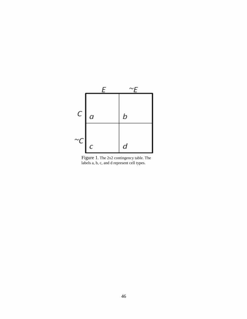
46

Figure 1. The 2x2 contingency table. The

labels a, b, c, and d represent cell types.

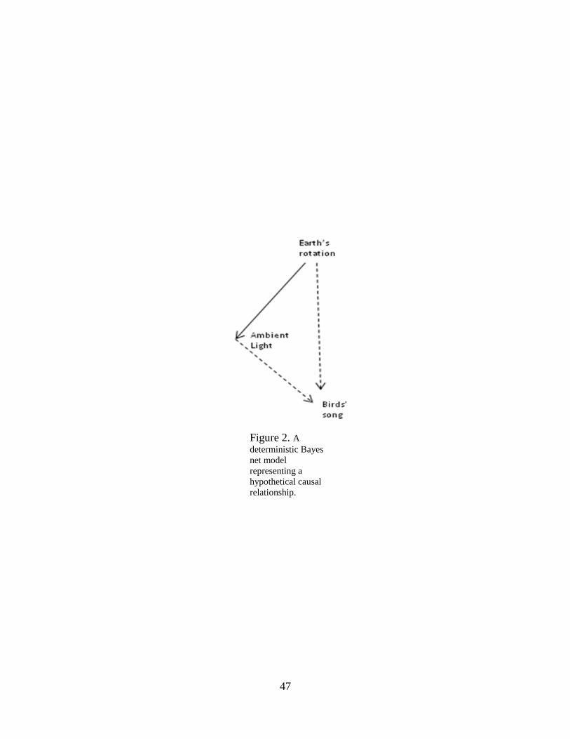
47

Figure 2. A

deterministic Bayes

net model

representing a

hypothetical causal

relationship.

48

Figure 3. Updated Bayes

net .representation of Fig. 2.

after graphy surgery.

49

Causal Judgment by Group

Initial Hypothesis

Positive Negative Control

Ca

usa

l Jud

gm

ent

0

30

40

50

60

70 Small Trial Number

Large Trial Number

Figure 4. Bars depict mean contingency ratings by group. Higher

scores denote higher causal ratings between the candidate cause and

effect in this experiment. Error bars represent standard error.

50

Causal Judgment by Hypothesis

Initial Hypothesis

Positive Negative Control

Causal Judgm

ent

0

30

40

50

60

70

Figure 5. Bars depict mean contingency ratings by group. Higher scores

denote higher causal ratings between the candidate cause and effect in

this experiment. Group means have been collapsed across the trial

number condition for this figure. Error bars represent standard error.

51

Absolute Estimates Cell A Cell B Cell C Cell D

Objective Frequency 9 3 3 9

Positive Low 8.05 (0.71) 4.89 (0.67) 5.47 (0.73) 6.05 (0.47)

Negative Low 8.16 (0.60) 4.79 (0.57) 4.95 (0.50) 6.42 (0.65)

Control Low 9.50 (1.08) 5.06 (0.55) 5.62 (1.04) 5.75 (0.48)

Table 1. Cell frequency estimates and SEM (in

parentheses) for the low trial size condition.

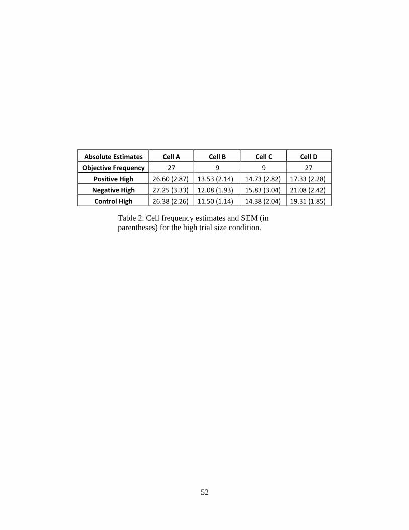
52

Absolute Estimates Cell A Cell B Cell C Cell D

Objective Frequency 27 9 9 27

Positive High 26.60 (2.87) 13.53 (2.14) 14.73 (2.82) 17.33 (2.28)

Negative High 27.25 (3.33) 12.08 (1.93) 15.83 (3.04) 21.08 (2.42)

Control High 26.38 (2.26) 11.50 (1.14) 14.38 (2.04) 19.31 (1.85)

Table 2. Cell frequency estimates and SEM (in

parentheses) for the high trial size condition.

53

References

Aitken, M., Larkin, M., & Dickinson, A. (2001). Re-examination of the role of within-compound

associations in the retrospective revaluation of causal judgments. Quarterly Journal of

Experimental Psychology, 54B, 27-51.

Allan, L. J. (1980). A note on measurement of contingency between two binary variables in

judgment tasks. Bulletin of the Psychonomic Society, 15, 147-149.

Allan, L. G. (1993). Human contingency judgments: Rule-based or associative? Psychological

Bulletin, 114, 435-448.

Alloy, L. B., & Abramson, L. Y. (1979). Judgment of contingency in depressed and

nondepressed students: Sadder but wiser? Journal of Experimental Psychology: General,

108, 441-485.

Arcediano, F., Matute, H., Escobar, M., & Miller, R. (2005). Competition between antecedent

and between subsequent stimuli in causal judgments. Journal of Experimental

Psychology: Learning, Memory, and Cognition, 31, 228-237.

Aristotle. (350 BCE). On Memory. In Ross, G. (Ed.) (1930). Aristotle: De Sensu and De

Memoria (vol. 3). Oxford: Oxford Press. (p. 452a 28)

Bacon, F. (1620). Novum organum. New York: P. F. Collier & Son.

Brunswik, E. (1955). In defense of probabilistic functionalism: a reply. Psychological Review,

62, 236-242.

Buehner, M., & May, J. (2003). Rethinking temporal contiguity and the judgment of causality:

effects of prior knowledge, experience, and reinforcement procedure. The Quarterly

Journal of Experimental Psychology, 56A, 865-890.

Busemeyer, J. R. (1991). Intuitive statistical information. In N.H. Anderson (Ed.), Contributions

to information integration theory (pp. 187-205). Hillsdale, N.J.: Erlbaum.

Catena, A., Maldonado, A., & Candido, A. (1998). The effect of frequency of judgment and the

type of trials on covariation learning. Journal of Experimental Psychology: Human

Perception and Performance, 24, 481-495.

Cheng, P. W. (1997). From covariation to causation: a causal power theory. Psychological

Review, 104, 367-405.

Cheng, P. W., & Novick, L. R. (1990). A probabilistic model of causal induction. Journal of

Personality and Social Psychology, 48(4), 545-567.

54

Cheng, P. W., & Novick, L. R. (1991). Causes versus enabling conditions. Cognition, 40, 83-

120.

Cheng, P. W., Park, J., Yarlas, A. S., Holyoak, K. J. (1996). A causal power theory of focal sets.

In D. R. Shanks, K. J. Holyoak, & D. L. Medin (Eds.), The psychology of learning and

motivation (Vol. 34, pp. 313-355). San Diego, CA: Academic Press.

Crocker, J. (1981). Judgment of covariation by social perceivers. Psychological Bulletin, 90,

272-292.

Darwin, C. (1859). The origin of species. London: John Murray.

Denniston, J.C., Miller, R.R., & Matute, H. (1996). Biological significance as determinant of cue

competition. Psychological Science, 7, 325-331.

Dickinson, A., & Burke, J. (1996). Within-compound associations mediate the retrospective

revaluation of causality judgements. Quarterly Journal of Experimental Psychology B:

Comparative and Physiological Psychology, 49B, 60-80.

Dickinson, A., Shanks, D.R., & Evenden, J.L. (1984). Judgment of act-outcome contingency: the

role of selective attribution. Quarterly Journal of Experimental Psychology, 36A, 29-50.

Evans, J.St.B.T. (1989). Biases in human reasoning: Causes and consequences. Hillsdale, NJ:

Erlbaum.

Faro, D., Leclerc, F., & Hastie, R. (2005). Percieved causality as a cue to temporal distance.

Psychological Science, 16, 673-677.

Flew, A. (1962). David Hume: On human nature and the understanding. New York: Macmillian.

Fischhoff, B., & Beyth-Marom, R. (1983). Hypothesis evaluation from a Bayesian perspective.

Psychological Review, 90, 239-260.

French, R.M. (2002). The computational modeling of analogy-making. Trends in Cognitive

Science, 6, 200-205.

Fugelsang, J., & Thompson, V. (2000). Strategy selection in causal reasoning: when beliefs and

covariation collide. Canadian Journal of Experimental Psychology, 54, 15-32.

Gluck, M., & Bower, G. (1988). From conditioning to category learning: an adaptive network

model. Journal of Experimental Psychology: General, 117, 227-247.

Glymour, C. (2000). Bayes nets as psychological models. In Kiel, F.C. & Wilson, R.A. (Eds.),

Explanation and cognition. Cambridge, (pp.169-190). Cambridge, MA: MIT Press.

55

Gopnik, A., & Glymour, C. (2002). Causal maps and Bayes nets: a cognitive and computational

account of theory-formation. In Carruthers, P., Stich, S.P., Siegal, M. (Eds.), The

cognitive basis of science. (pp. 117-132). Cambridge, MA: MIT Press.

Gopnik, A., Glymour, C., Sobel, D., Schulz, L., Kushnir, T., & Danks, D. (2004). A theory of

causal learning in children: causal maps and Bayes nets. Psychological Review, 111, 3-

32.

Griffiths, T., & Tenenbaum, J. (2005). Structure and strength in causal induction. Cognitive

Psychology, 51, 334-384.

Hagmayer, Y., & Waldmann, M. (2007). Inferences about unobserved causes in human

contingency learning. The Quarterly Journal of Experimental Psychology, 60, 330-355.

Hempel, C. (1945). Studies in the logic of confirmation. Mind, 54, 1-26.

Hergenhahn, B.R. (2005). An Introduction to the History of Psychology. Belmont, CA: Thomson

Wadsworth.

Holyoak, K.J., Thagard, P. (1997). The analogical mind. American Psychologist, 52, 35-44.

Hume, D. (1747). An Enquiry Concerning Human Understanding. New York: Forgotten Books.

Inhelder, B., & Piaget, J. (1958). The growth of logical thinking from childhood to adolescence.

New York, NY: Basic Books.

Jenkins, H.M., & Ward, W.C. (1979). Judgment of contingency between responses and

outcomes. Psychological Monographs, 79, 1-17.

Kahneman, D., & Tversky, A. (1973). On the psychology of prediction. Psychological Review,

80, 237-251.

Kant, I. (1781). Critique of Pure Reason. New York: P. F. Collier & Son.

Kao, S.F., & Wasserman, E.A. (1993). Assessment of an information integration account of

contingency judgment with examination of subjective cell importance and method of

information presentation. Journal of Experimental Psychology: Learning, Memory, and

Cognition, 19, 1363-1386.

Klayman, J., & Ha, Y.W. (1987). Confirmation, disconfirmation, and information in hypothesis

testing. Psychological Review, 94, 211-228.

Liljeholm, M., & Cheng, P. (2007). When is a cause the „same‟?: coherent generalization across

contexts. Psychological Science, 18, 1014-1021.

56

Levin, I.P., Wasserman, E.A., and Kao, S.F. (1993). Multiple methods for examining biased

information use in contingency judgments. Organizational Behavior and Human

Decision Processes, 55, 228-250.

Lien, Y., & Cheng, P. W. (2000). Distinguishing genuine from spurious causes: a coherence

hypothesis. Cognitive Psychology, 40, 87-137.

Lovibond, P. (2003). Causal beliefs and conditioned responses: retrospective revaluation induced

by experience and by instruction. Journal of Experimental Psychology: Learning,

Memory, and Cognition, 29, 97-106.

Marr, D. (1982). The philosophy and the approach. In Vision: A computational investigation into

the human representation and processing of visual information (chap. 1). San Francisco,

CA: Freeman.

Mackintosh, N. (1975). A theory of attention: variations in the associability of stimuli with

reinforcement. Psychological Review, 82, 276-298.

Medin, D., & Edelson, S. (1988). Problem structure and the use of base-rate information from

experience. Journal of Experimental Psychology: Experimental, 117, 68-85.

Miller, R.R., Hallam, S., & Grahame, N. (1990). Inflation of comparator stimuli following CS

training. Animal Learning & Behavior, 18, 434-443.

Mitchell, C., Lovibond, P., Minard, E., & Lavis, Y. (2006). Forward blocking in human learning

sometimes reflects the failure to encode a cue-outcome relationship. The Quarterly

Journal of Experimental Psychology, 59, 830-844.

Nickerson, R.S. (1998). Confirmation Bias: A ubiquitous phenomenon in many guises. Review of

General Psychology, 2, 175-220.

Pearl, J. (2000). Causality: Models, Reasoning, and Inference. Cambridge: Cambridge

University Press.

Pearce, J.M. (1987). A model for stimulus generalization in Pavlovian conditioning.


Pearce, J., & Hall, G. (1980). A model for Pavlovian learning: variations in the effectiveness of

conditioned but not of unconditioned stimuli. Psychological Review, 87, 532-552.

Perales, J.C., & Shanks, D.R. (2007). Models of covariation-based causal judgment: A review

and synthesis. Psychonomic Bulletin & Review, 14, 577-596.

Peterson, C.R., & Beach, L.R. (1967). Man as an intuitive statistician. Psychological Bulletin,

68, 29-46.

57

Popper, K. (1969). Conjectures and Refutations. London: Routledge and Kegan Paul.

Reips, U-D., & Waldmann, M. (2008). When learning order affects sensitivity to base rates:

challenges for theories of causal learning. Experimental Psychology, 55, 9-22.

Rescorla, R.A., & Wagner, A.R. (1972) A theory of Pavlovian conditioning: Variations in the

effectiveness of reinforcement and nonreinforcement. In A.H. Black & W.F. Prokasy

(Eds.), Classical conditioning: II. Current research and theory (pp. 64-99). New York:

Appleton-Century-Crofts.

Schweitzer, L., & Green, L. (1982). Reevaluation of things past: a test of the „retrospection

hypothesis‟ using a CER procedure with rats. Pavlovian Journal of Biological Science,

17, 62-68.

Schulz, L., & Sommerville, J. (2006). God does not play dice: causal determinism and

preschoolers‟ causal inferences. Child Development, 77, 427-442.

Shaklee, H., & Mims, M. (1981). Development of rule use in judgments of covariation between

events. Child Development, 52, 317-325.

Shaklee, H., & Tucker, D. (1980). A rule analysis of judgments of covariation between events.

Memory & Cognition, 8, 459-467.

Smedslund, J. (1963). The concept of correlation in adults. Scandinavian Journal of Psychology,

4, 165-173.

Spellman, B.A. (1996). Conditionalizing causality. In D. R. Shanks, K. J. Holyoak, & D. L.

Medin (Eds.), The psychology of learning and motivation (Vol. 34, pp. 167-205). San

Diego, CA: Academic Press.

Stout, S., & Miller, R.R. (2007). Sometimes-competing retrieval (SOCR): a formalization of the

comparator hypothesis. Psychological Review, 114, 759-783.

Tolman, E.C., & Brunswik, E. (1935). The organism and the causal texture of the environment.


Tversky, A., & Kahneman, D. (1980). Causal schemas in judgments under uncertainty. In M.

Fishbein (Ed.), Progress in Social Psychology (pp. 49-72). Hillsdale, NJ: Erlbaum

Tversky, A., & Koehler, D. (1994). Support theory: a nonextension representation of subjective

probability. Psychological Review, 101, 547-567.

Vadillo, M.A., Miller, R.R., & Matute, H. (2005). Causal and predictive-value judgments, but

not predictions, are based on cue—outcome contingency. Learning & Behavior, 33, 172-

183.

58

Van Hamme, L., & Wasserman, E. (1994). Cue competition in causality judgments: the role of

nonpresentation of compound stimulus elements. Learning & Motivation, 25, 127-151.

Ward, W., & Jenkins, H. (1965). The display of information and the judgment of contingency.

Canadian Journal of Psychology, 19, 231-241.

Waldmann, M. (1996). Determining whether causal order affects cue selection in human

contingency learning: comments on Shanks and Lopez (1996). Memory & Cognition, 25.

Waldmann, M. (2000). Competition between causes but not effects in predictive and diagnostic

learning. Journal of Experimental Psychology: Learning, Memory, and Cognition, 26,

53-76.

Waldmann, M. (2001). Predictive versus diagnostic causal learning: evidence from an

overshadowing paradigm. Psychonomic Bulletin & Review, 8, 600-608.

Waldmann, M., & Hagmayer, Y. (2005). Seeing versus doing: two modes of accessing causal

knowledge. Journal of Experimental Psychology: Learning, Memory, and Cognition, 31,

216-227.

Waldmann, M., & Hagmayer, Y. (2006). Categories and causality: the neglected direction.

Cognitive Psychology, 53, 27-58.

Waldmann, M., & Holyoak, K. (1992). Predictive and diagnostic learning within causal models:

asymmetries in cue competition. Journal of Experimental Psychology: General, 121,

222-236.

Waldmann, M., Holyoak, K., & Fratianne, A. (1995). Causal models and the acquisition of

category structure. Journal of Experimental Psychology: General, 124, 181-206.

Waldmann, M.R. (1996). Knowledge-based causal induction. In D. R. Shanks, K. J. Holyoak, &

D. L. Medin (Eds.), The psychology of learning and motivation (Vol. 34, pp. 167-205).

San Diego, CA: Academic Press.

Wason, P.C. (1960). On the failure to eliminate hypotheses in a conceptual task. Quarterly

Journal of Experimental Psychology, 12, 129-140.

Wasserman, E.A., Dorner, W.W., Kao, S.F. (1990). Contributions of specific cell information to

judgments of interevent contingency. Journal of Experimental Psychology: Learning,

Memory, and Cognition, 16, 509-521.

White, P. (2000). Causal judgment from contingency information: relation between subjective

reports and individual tendencies in judgment. Memory & Cognition, 28, 415-426.

59

White, P. (2003). Making causal judgments from the proportion of confirming instances: the pCI

rule. Journal of Experimental Psychology: Learning, Memory, and Cognition, 29, 710-

727.

Documents

Initially Held Hypothesis Does Not Affect Encoding of