Inhibiting Shear Instability Induced by Large …wychoi/pub/SAPM_09_2.pdfInhibiting Shear Instability Induced by Large Amplitude Internal Solitary Waves in Two-Layer Flows with a Free

Inhibiting Shear Instability Induced by Large AmplitudeInternal Solitary Waves in Two-Layer Flows

with a Free Surface

By Ricardo Barros and Wooyoung Choi

We consider a strongly nonlinear long wave model for large amplitude internalwaves in two-layer flows with the top free surface. It is shown that the modelsuffers from the Kelvin–Helmholtz (KH) instability so that any given shear(even if arbitrarily small) between the layers makes short waves unstable.Because a jump in tangential velocity is induced when the interface isdeformed, the applicability of the model to describe the dynamics of internalwaves is expected to remain rather limited. To overcome this major difficulty,the model is written in terms of the horizontal velocities at the bottom and theinterface, instead of the depth-averaged velocities, which makes the systemlinearly stable for perturbations of arbitrary wavelengths as long as the sheardoes not exceed a certain critical value.

1. Introduction

Large amplitude oceanic internal waves is a ubiquitous phenomenon that despitebeing known for centuries, has only been recently the subject of scientificstudies. They manifest on the surface of the sea by long isolated stripes ofhighly agitated features that are defined as audibly breaking waves and white

Address for correspondence: W. Choi, Department of Mathematical Sciences and Center for AppliedStatistics, New Jersey Institute of Technology, Newark, NJ 07102-1982, USA; e-mail: [email protected]

STUDIES IN APPLIED MATHEMATICS 122:325–346 325C© 2009 by the Massachusetts Institute of Technology

326 R. Barros and W. Choi

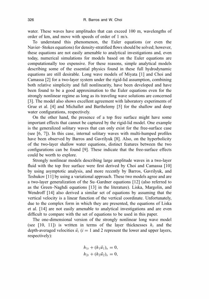
water. These waves have amplitudes that can exceed 100 m, wavelengths oforder of km, and move with speeds of order of 1 m/s.

To understand this phenomenon, the Euler equations (or even theNavier–Stokes equations) for density-stratified flows should be solved; however,these equations are not easily amenable to analytical investigations and, eventoday, numerical simulations for models based on the Euler equations arecomputationally too expensive. For these reasons, simple analytical modelsdescribing some of the essential physics found in these full hydrodynamicequations are still desirable. Long wave models of Miyata [1] and Choi andCamassa [2] for a two-layer system under the rigid-lid assumption, combiningboth relative simplicity and full nonlinearity, have been developed and havebeen found to be a good approximation to the Euler equations even for thestrongly nonlinear regime as long as its traveling wave solutions are concerned[3]. The model also shows excellent agreement with laboratory experiments ofGrue et al. [4] and Michallet and Barthelemy [5] for the shallow and deepwater configurations, respectively.

On the other hand, the presence of a top free surface might have someimportant effects that cannot be captured by the rigid-lid model. One exampleis the generalized solitary waves that can only exist for the free-surface case(see [6, 7]). In this case, internal solitary waves with multi-humped profileshave been observed by Barros and Gavrilyuk [8]. Also, on the hyperbolicityof the two-layer shallow water equations, distinct features between the twoconfigurations can be found [9]. These indicate that the free-surface effectscould be worth to explore.

Strongly nonlinear models describing large amplitude waves in a two-layerfluid with the top free surface were first derived by Choi and Camassa [10]by using asymptotic analysis, and more recently by Barros, Gavrilyuk, andTeshukov [11] by using a variational approach. These two models agree and area two-layer generalization of the Su–Gardner equations [12] (also referred toas the Green–Naghdi equations [13] in the literature). Liska, Margolin, andWendroff [14] also derived a similar set of equations by assuming that thevertical velocity is a linear function of the vertical coordinate. Unfortunately,due to the complex form in which they are presented, the equations of Liskaet al. [14] are not easily amenable to analytical investigations and are evendifficult to compare with the set of equations to be used in this paper.

The one-dimensional version of the strongly nonlinear long wave model(see [10, 11]) is written in terms of the layer thicknesses hi and thedepth-averaged velocities ui (i = 1 and 2 represent the lower and upper layers,respectively):

h1t + (h1u1)x = 0,

h2t + (h2u2)x = 0,

Inhibiting Shear Instability Induced by Internal Solitary Waves 327

u1t + u1u1x + g(h1 + ρh2)x + ρ

(−1

2G2h2

2 + (D2

2h1)h2

)x

= 1

3h1

(h3

1G1)

x,

u2t + u2u2x + g(h1 + h2)x = 1

3h2

(h2

3G2)

x− 1

2h2

(h2

2 D22h1

)x

+(

1

2h2G2 − D2

2h1

)h1x . (1)

where g is the gravitational acceleration, ρi are the fluid densities with ρ2 < ρ1

for stable stratification, and the subscripts x and t represent partial differentiationwith respect to space and time, respectively. We have also introduced thedensity ratio ρ < 1 defined by ρ = ρ2/ρ1, the second-order material derivativeof h1 with respect to the averaged velocity field u2 denoted here by D2

2h1,where D2 = ∂t + u2∂x , and the nonlinear dispersive terms Gi given by

Gi = ui xt + ui ui xx − ui x2.

The system is endowed with a Hamiltonian structure and the momentumequations can be found as the Euler–Lagrange equations for an approximateLagrangian to the Euler equations for two-layer flows with the free surface [11].This same structure holds also for its traveling-wave solutions, which revealedin [8] as a valuable tool to characterize these solutions. In their paper, Barrosand Gavrilyuk [8] have shown quite a rich diversity of solitary-wave solutionsthat is absent in the rigid-lid case. In particular, the multi-humped solitary-wavesolutions exhibited there show the richness and complexity of the Hamiltoniansystem with two degrees of freedom describing traveling-wave solutions.

Unfortunately, a major difficulty is expected in solving numerically thismodel for the study of the propagation of solitary waves. Although nobackground shear is present when the interface is flat, a jump in tangentialvelocity, leading to a Kelvin–Helmholtz (KH) instability, is induced whenthe interface is deformed since the model was derived under the inviscidassumption, which requires only continuity of normal velocity. The samedifficulty is present for the rigid-lid configuration, as pointed out by Jo andChoi [15]. In an attempt to overcome this difficulty, Jo and Choi [16] proposedthe use of a low-pass filter to remove unstable short waves which enables oneto simulate the propagation of a single solitary wave of large amplitude for along time. The drawback of this approach is the difficulty of applying the sametechnique to general time-dependent problems.

A recent work by Choi, Barros, and Jo [17] addresses the problem with morepromising results for a two-layer system bounded by rigid walls. Adoptingthe idea of Nguyen and Dias [18] for a weakly nonlinear model, Choiet al. [17] expressed the strongly nonlinear model in terms of the horizontalvelocities at certain preferred vertical levels, instead of the depth-averagedvelocities. Through local stability analysis under the assumption that the


velocity jump varies slowly in space, it was shown that the new form of thestrongly nonlinear model changes the dispersion relation in a way that internalsolitary waves become stable to perturbations of arbitrary wavelengths as longas their amplitudes do not exceed a certain critical value. In fact, this criticalamplitude is found to be close enough to the maximum amplitude for a widerange of physical parameters, which opens the possibility of using the modelfor real applications in the strongly nonlinear regime.

In this paper, we will first show that our original strongly nonlinear modelwith the top free surface suffers from the KH instability. Then, following Choiet al. [17], we propose a strongly nonlinear model that is asymptoticallyequivalent to the original one, but has a different dispersive behavior for shortwaves. Compared with the rigid-lid model, the free-surface model given by (1)yields a much more complex dispersion relation due to the two extra degrees offreedom. It will be shown analytically that, by considering the velocities at thebottom and the interface, the dispersion relation is modified in a way that thisKH instability is contained up to a certain critical shear between the layers.

2. Shear instability for the original strongly nonlinear model

By looking for solutions (h1, h2, u1, u2) ∼ exp[i(kx − ωt)] of the system ofEquations (1) linearized about ui = Ui and hi = H i, we obtain the followinglinear dispersion relation between ω and k:[(

1 + 1

3k2 H 2

1

)(c − U1)2 − gH1

] [(1 + 1

3k2 H 2

2

)(c − U2)2 − gH2

]

+ ρH1 H2

[k2

(1 + 1

12k2 H 2

2

)(c − U2)4 − g2

]= 0, (2)

where k is the wave number, ω is the wave frequency, and c = ω/k is the wavespeed. In (2), the horizontal velocities U i induced by a slowly varying solitarywave are assumed to be locally constant. We will prove that, for any given shearbetween layers, there exists a critical wave number kcr such that Equation (2)has complex roots for k >kcr. This implies that the strongly nonlinear internalwave model (1) is always linearly unstable to short-wavelength perturbations.To prove this, we write Equation (2) in terms of nondimensional variables:

c = c√gH1

, H = H2

H1, K = k H1, F = U2 − U1√

gH1, (3)

and assume without loss of generality that u1/√

gH1 = 1 (by choosing amoving reference frame such this condition is met). Then, the dispersionrelation becomes

a0c 4 + a1c 3 + a2c 2 + a3c + a4 = 0, (4)


where the coefficients are functions of ρ, H , F, and K (see Appendix A). Weremark that the strongly nonlinear model under the rigid-lid approximationyields a quadratic equation for the wave speed c. In the free-surface case, asa consequence of the two extra degrees of freedom, the dispersion relationbecomes a quadratic equation. For this equation, we seek relations involvingthese parameters for which Equation (4) has only real roots. Notice that thesystem is always linearly stable for F = 0 since the dispersion relation (2)reduces to a biquadratic form with four distinct real solutions (see [8]).

Several attempts have been made in the past to obtain conditions in terms ofthe literal coefficients of a polynomial, concerning a special root distribution (see[19] and references therein). Among them, Jury and Mansour [19] presented aseries of algorithms involving characteristic expressions for a quartic equation,allowing a full characterization of the root distribution in a much more conciseform than the one provided by previous approaches. Similar criteria involvingonly inner determinants were also obtained by Fuller [20]. Following thiselegant exposition, when considering the inner determinants 3, 5, 7:1

7 =

a0 a1 a2 a3 a4 0 0

0 a0 a1 a2 a3 a4 0

0 0 a0 a1 a2 a3 a4

0 0 0 4a0 3a1 2a2 a3

0 0 4a0 3a1 2a2 a3 0

0 4a0 3a1 2a2 a3 0 0

4a0 3a1 2a2 a3 0 0 0

,

with 3 and 5 being defined as the determinants of the inner matrices withdimensions 3 × 3 and 5 × 5, respectively (as denoted by the two inner squaresin the definition of 7), we have the following result (see [20], p. 778):

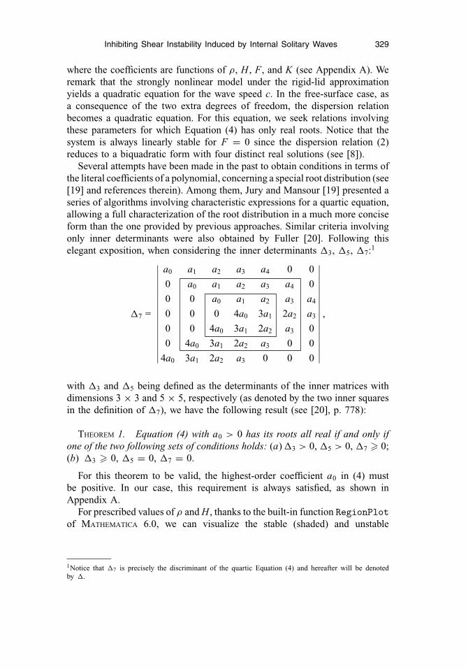
THEOREM 1. Equation (4) with a0 > 0 has its roots all real if and only ifone of the two following sets of conditions holds: (a) 3 > 0, 5 > 0, 7 � 0;(b) 3 � 0, 5 = 0, 7 = 0.

For this theorem to be valid, the highest-order coefficient a0 in (4) mustbe positive. In our case, this requirement is always satisfied, as shown inAppendix A.

For prescribed values of ρ and H , thanks to the built-in function RegionPlotof MATHEMATICA 6.0, we can visualize the stable (shaded) and unstable

1Notice that 7 is precisely the discriminant of the quartic Equation (4) and hereafter will be denotedby .


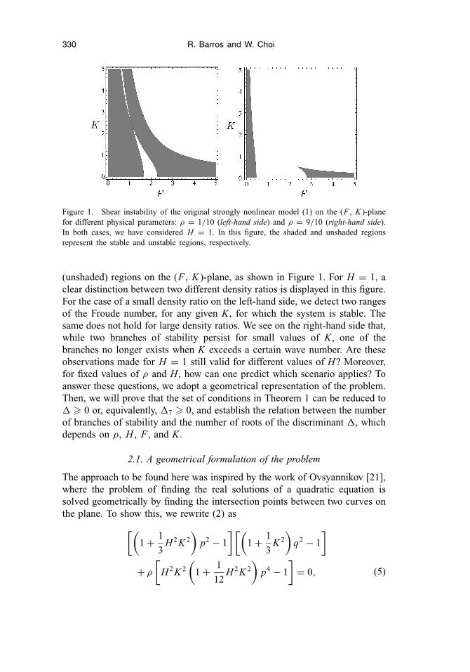
Figure 1. Shear instability of the original strongly nonlinear model (1) on the (F , K )-planefor different physical parameters: ρ = 1/10 (left-hand side) and ρ = 9/10 (right-hand side).In both cases, we have considered H = 1. In this figure, the shaded and unshaded regionsrepresent the stable and unstable regions, respectively.

(unshaded) regions on the (F , K )-plane, as shown in Figure 1. For H = 1, aclear distinction between two different density ratios is displayed in this figure.For the case of a small density ratio on the left-hand side, we detect two rangesof the Froude number, for any given K, for which the system is stable. Thesame does not hold for large density ratios. We see on the right-hand side that,while two branches of stability persist for small values of K, one of thebranches no longer exists when K exceeds a certain wave number. Are theseobservations made for H = 1 still valid for different values of H? Moreover,for fixed values of ρ and H , how can one predict which scenario applies? Toanswer these questions, we adopt a geometrical representation of the problem.Then, we will prove that the set of conditions in Theorem 1 can be reduced to � 0 or, equivalently, 7 � 0, and establish the relation between the numberof branches of stability and the number of roots of the discriminant , whichdepends on ρ, H , F , and K.

2.1. A geometrical formulation of the problem

The approach to be found here was inspired by the work of Ovsyannikov [21],where the problem of finding the real solutions of a quadratic equation issolved geometrically by finding the intersection points between two curves onthe plane. To show this, we rewrite (2) as

[(1 + 1

3H 2 K 2

)p2 − 1

] [(1 + 1

3K 2

)q2 − 1

]

+ ρ

[H 2 K 2

(1 + 1

12H 2 K 2

)p4 − 1

]= 0, (5)


by defining

c − U1 = q√

gH1, c − U2 = p√

gH2. (6)

As a consequence of (6), it can be noticed that p and q are related by

q =√

H p + F, (7)

and, therefore, finding the solutions of (2) is equivalent to finding the solutionsof the system of equations for p and q given by (5) and (7).

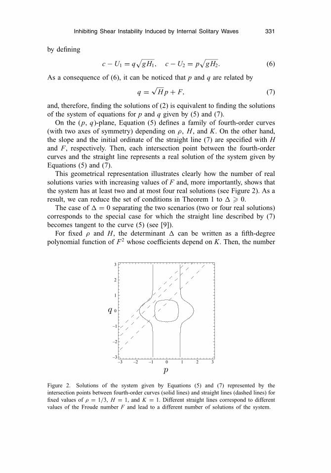
On the (p, q)-plane, Equation (5) defines a family of fourth-order curves(with two axes of symmetry) depending on ρ, H , and K. On the other hand,the slope and the initial ordinate of the straight line (7) are specified with Hand F, respectively. Then, each intersection point between the fourth-ordercurves and the straight line represents a real solution of the system given byEquations (5) and (7).

This geometrical representation illustrates clearly how the number of realsolutions varies with increasing values of F and, more importantly, shows thatthe system has at least two and at most four real solutions (see Figure 2). As aresult, we can reduce the set of conditions in Theorem 1 to � 0.

The case of = 0 separating the two scenarios (two or four real solutions)corresponds to the special case for which the straight line described by (7)becomes tangent to the curve (5) (see [9]).

For fixed ρ and H , the determinant can be written as a fifth-degreepolynomial function of F2 whose coefficients depend on K. Then, the number

–3 –2 –1 0 1 2 3–3

–2

–1

0

1

2

3

q

p

Figure 2. Solutions of the system given by Equations (5) and (7) represented by theintersection points between fourth-order curves (solid lines) and straight lines (dashed lines) forfixed values of ρ = 1/3, H = 1, and K = 1. Different straight lines correspond to differentvalues of the Froude number F and lead to a different number of solutions of the system.


0 1 2 3 4 50.0

0.2

0.4

0.6

0.8

1.0

ρ

K0 5 10 15 20

0.0

0.2

0.4

0.6

0.8

1.0

K

ρ

0 50 100 1500.0

0.2

0.4

0.6

0.8

1.0

ρ

K

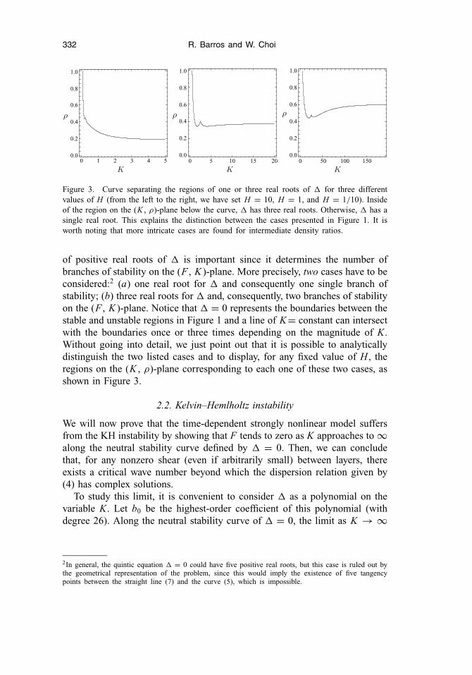
Figure 3. Curve separating the regions of one or three real roots of for three differentvalues of H (from the left to the right, we have set H = 10, H = 1, and H = 1/10). Insideof the region on the (K , ρ)-plane below the curve, has three real roots. Otherwise, has asingle real root. This explains the distinction between the cases presented in Figure 1. It isworth noting that more intricate cases are found for intermediate density ratios.

of positive real roots of is important since it determines the number ofbranches of stability on the (F , K )-plane. More precisely, two cases have to beconsidered:2 (a) one real root for and consequently one single branch ofstability; (b) three real roots for and, consequently, two branches of stabilityon the (F , K )-plane. Notice that = 0 represents the boundaries between thestable and unstable regions in Figure 1 and a line of K= constant can intersectwith the boundaries once or three times depending on the magnitude of K.Without going into detail, we just point out that it is possible to analyticallydistinguish the two listed cases and to display, for any fixed value of H , theregions on the (K , ρ)-plane corresponding to each one of these two cases, asshown in Figure 3.

2.2. Kelvin–Hemlholtz instability

We will now prove that the time-dependent strongly nonlinear model suffersfrom the KH instability by showing that F tends to zero as K approaches to ∞along the neutral stability curve defined by = 0. Then, we can concludethat, for any nonzero shear (even if arbitrarily small) between layers, thereexists a critical wave number beyond which the dispersion relation given by(4) has complex solutions.

To study this limit, it is convenient to consider as a polynomial on thevariable K. Let b0 be the highest-order coefficient of this polynomial (withdegree 26). Along the neutral stability curve of = 0, the limit as K → ∞

2In general, the quintic equation = 0 could have five positive real roots, but this case is ruled out bythe geometrical representation of the problem, since this would imply the existence of five tangencypoints between the straight line (7) and the curve (5), which is impossible.


leads to b0 = 0. Since b0 is given by

b0 = −147456 ρ (4 + 3ρH )H 14 F10,

we conclude that this can happen only if F = 0, and so the result follows.Whenever the interface is displaced from its equilibrium position, a jump in

tangential velocity is induced in the strongly nonlinear model. Therefore, themodel becomes ill-posed and not suited for the numerical study of the dynamicsof large amplitude internal solitary waves. To overcome this difficulty, wewill adopt the idea of Choi et al. [17] for the rigid-lid model and derive aregularized free-surface model that inhibits this KH instability.

3. Derivation of a regularized model

In this section, we will derive a new strongly nonlinear model that isasymptotically equivalent to the original model (1), but has a different dispersivebehavior for short waves. The strategy presented here is similar to the one foundin [17], where the depth-averaged velocities ui in the original equations arereplaced by ui , the velocities evaluated at certain vertical levels zi , neglectingall the terms of O(ε4) or higher, where ε is the small parameter representingthe ratio of a typical vertical scale to a typical horizontal scale. First, we willshow how the velocities ui and ui are related. Then, using this relationship, wewill propose a new model to describe large amplitude internal solitary wavesand, by means of local stability analysis, show that the KH instability canindeed be suppressed up to a certain critical shear between layers.

3.1. Relationship between the depth-averaged velocities and the horizontalvelocities at particular depth levels

We first consider the mass conservation laws in nondimensional variables:

uix + wi z = 0, (8)

where the vertical coordinate z is measured upward from the flat bottom. Weassume, accordingly to Choi and Camassa [10], that the components f = (ui,wi) of the vector velocity can be asymptotically expanded as

f (x, z, t) = f (0) + ε2 f (1) + O(ε4).

Set i = 1 and integrate (8), using the boundary condition w1(x , z = 0, t) = 0,to obtain

w1 = −z u(0)1x − ε2

∫ z

0u(1)

1x dz + O(ε4).


It follows that the leading order of the vertical velocity is given by

w(0)1 = −z u(0)

1x .

Assuming that the flow is irrotational so that

uiz = ε2wi x ,

or equivalently

u(1)1z = w

(0)1x ,

leads to the relation

u(1)1z = −z u(0)

1xx ,

which can be integrated to produce

u(1)1 = u1

∣∣z=0

− 1

2u(0)

1xx z2.

Combining the results, we may write

u1 = u(0)1 + ε2

(−1

2u(0)

1xx z2

)+ O(ε4), (9)

where the value of the horizontal velocity at the bottom is irrelevant here sinceit can be absorbed by the leading-order term (that is only a function of x andt). By the definition of the depth-averaged velocities, it follows that

u1 = u(0)1 + ε2

(−1

6u(0)

1xx h21

)+ O(ε4).

On the other hand, we can deduce from (9) that the horizontal velocity u1 isevaluated at a particular level 0 � z1 � h1(x, t):

u1 = u(0)1 + ε2

(−1

2u(0)

1xx z21

)+ O(ε4).

As a result, the following relation between u1 and u1 holds:

u1 = u1 + ε2

(−1

2u1xx z2

1 + 1

6u1xx h2

1

)+ O(ε4),

which we can write in dimensional variables as

u1 = u1 + 1

2u1xx z2

1 − 1

6u1xx h2

1 + O(ε4). (10)


We proceed in a completely analogous way with the lighter fluid (i = 2).This time, we integrate (8) to obtain

w2 = w2∣∣

z=h1

− (z − h1) u(0)2x − ε2

∫ z

h1

u(1)2x dz + O(ε4),

which is precisely

w(0)2 = −u(0)

2x (z − h1) + h1t + u(0)2 h1x ,

when the kinematic boundary condition is imposed at the interface. Using thefact that the flow is irrotational allows us to write

u(1)2z = −u(0)

2xx (z − h1) + g(x, t),

with g(x , t) defined by

g(x, t) = u(0)2x h1x + (

h1t + u(0)2 h1x

)x.

Integrating the last relation leads to

u(1)2 = u2

∣∣z=h1

− 1

2u(0)

2xx (z − h1)2 + g(x, t) (z − h1),

and, considering that the integration constant is irrelevant, as mentioned before,we may write

u2 = u(0)2 + ε2

(−1

2u(0)

2xx (z − h1)2 + g(x, t) (z − h1)

)+ O(ε4). (11)

By the definition of the depth-averaged velocities, we have

u2 = u(0)2 + ε2

(−1

6u(0)

2xx h22 + 1

2g(x, t) h2

)+ O(ε4).

On the other hand, we know from (11) that at a particular vertical levelh1 � z2 � (h1 + h2), the horizontal velocity u2 is given by

u2 = u(0)2 + ε2

(−1

2u(0)

2xx (z2 − h1)2 + g(x, t) (z2 − h1)

)+ O(ε4),

and consequently

u2 = u2 + ε2

(− 1

2u2xx (z2 − h1)2 + g(x, t) (z2 − h1)

+ 1

6u2xx h2

2 − 1

2g(x, t) h2

)+ O(ε4),


where we have introduced g(x, t) defined by

g(x, t) = u2x h1x + (h1t + u2h1x )x .

This establishes the desired relation between u2 and u2:

u2 = u2 + 1

2u2xx (z2 − h1)2 − 1

6u2xx h2

2 − g(x, t) (z2 − h1)

+ 1

2g(x, t) h2 + O(ε4). (12)

We point out that we have not used here the fact that zi = constant. Nothingprevents us from considering zi = zi (x, t), and, therefore, any vertical level zi

including z = 0, z = h1(x , t) or z = (h1 + h2)(x , t) can be chosen, wheneverapplicable.

3.2. Derivation of an asymptotically equivalent model with an improveddispersion relation

We go back to (1) and substitute the expressions (10) and (12) for u1 and u2.Neglecting all the terms of O(ε4) or higher will provide a new system ofnonlinear evolution equations for hi and ui . We start with the mass conservationlaw for the heavier fluid that leads to

h1t +[

h1

(u1 + 1

2z2

1 u1xx − 1

6h2

1 u1xx

)]x

= 0. (13)

Considering the mass conservation law for the lighter fluid demands care.Substituting (12) straightforwardly into the second equation in (1) includesindirectly some higher-order terms since the expression of g(x, t) contains theterm h1t that can be expressed from (13) as

h1t = −(h1u1)x + O(ε2). (14)

To preserve asymptotic consistency in the way chosen to perturb thedispersive behavior for short waves, we should write for the lighter fluid

h2t +[

h2

(u2 + 1

2(z2 − h1)2 u2xx − 1

6h2

2 u2xx

− f (x, t)(z2 − h1) + 1

2f (x, t)h2

)]x

= 0, (15)

with f (x, t) given by

f (x, t) = u2x h1x + [[h1(u2 − u1)]x − h1u2x ]x .


Similarly, the momentum equation for the heavier fluid yields

u1t + u1u1x + g(h1 + ρh2)x =[

1

2h2

1 G1 + ρ

(1

2h2

2 G2 − ˆ(D2

2h1)h2

)]x

− 1

2z2

1 (u1xt + u1u1xx )x − (z1t + u1 z1x )z1u1xx ,

(16)

where the terms Gi and ˆ(D22h1) are defined as follows:

Gi = ui xt + ui ui xx − u2i x ,

ˆ(D2

2h1) = [−(h1u1)x (u2 − u1) + h1(u2 − u1)t ]x

+u2 [h1(u2 − u1)]xx + (h1u1)x u2x − h1u2xt − u2(h1u2x )x .

Finally, taking into account all the considerations made above, we have forthe lighter fluid the following equation:

u2t + u2 u2x + g(h1 + h2)x + 1

2(z2 − h1)2(u2xt + u2 u2xx )x

+ [z2t + u2 z2x − [h1(u2 − u1)]x + h1u2x ](z2 − h1)u2xx

+(

−(z2 − h1) + 1

2h2

)F(x, t) −

[z2t +

(h1u1 + 1

2h2u2

)x

]f (x, t)

+[

u2

(− f (x, t)(z2 − h1) + 1

2f (x, t)h2

)]x

=(

1

2h2

2G2

)x

− ˆ(D2

2h1)h2x

− 1

2h2

ˆ(D2

2h1)

x+

(1

2h2G2 − ˆ(

D22h1

))h1x , (17)

where F(x, t) is precisely the partial time derivative f t (x, t) written, byconsidering (14), as:

F(x, t) = u2xt h1x − u2x (h1u1)xx + [−(h1u1)x (u2 − u1) + h1(u2 − u1)t ]xx

− [−(h1u1)x u2x + h1u2xt ]x .

3.3. Local stability analysis

Using local stability analysis, we will investigate how the vertical levels inthe new model formed by Equations (13) and (15)–(17) should be chosen toinhibit the shear instability induced by internal solitary waves. By substitutinginto these equations hi = Hi + h′

i and ui = Ui + u′i and assuming the prime

variables are small, the system linearized about ui = U i and hi = H i is given,after dropping the primes, by

h1t + U1h1x + H1u1x + α1 H 31 u1xxx = 0, (18)


h2t + U2h2x + H2u2x + α2 H 32 u2xxx

+(

1

2− θ2

)H 2

2 [(U2 − U1)h1xxx − H1u1xxx ] = 0, (19)

u1t + U1u1x + g(h1 + ρh2)x +[(

α1 − 1

3

)H 2

1 − ρH1 H2

]u1xxt

+[U1

(α1− 1

3

)H 2

1 +ρH1 H2(U1 − 2U2)

]u1xxx

− 1

2ρH 2

2 (u2xxt + U2u2xxx )

+ ρH2(U2 − U1)2 h1xxx = 0,

(20)

u2t + U2u2x + g(h1 + h2)x +(

α2 − 1

3

)H 2

2 (u2xxt + U2u2xxx )

+ H2

(θ2 − 1

2

)[H1(U2 − U1)u1xxx + U1(U2 − U1)h1xxx

+ H1u1xxt ] − H2U2

(θ2 − 1

2

)[(U2 − U1)h1xxx − H1u1xxx ]

+ 1

2H2[(U2 − U1)2h1xxx + H1(U1−2U2)u1xxx − H1u1xxt ] = 0,

(21)where we have introduced

θ1 = z1

H1, θ2 = z2 − H1

H2, α1 = 1

2θ2

1 − 1

6, α2 = 1

2θ2

2 − 1

6.

By definition, 0 ≤ θ i ≤ 1 and, for example, both θ1 and θ2 are zero whenz1 = 0 and z2 = H1, that corresponds to prescribing the vertical levels at thebottom and the interface, respectively. It is worth to note that, in contrastwith the rigid-lid case [17], there are no preferred levels for which the lineardispersion relation obtained for the original strongly nonlinear model (writtenin terms of the depth averaged velocities) is recovered.

By looking for solutions (h1, h2, u1, u2) ∼ exp[i(kx − ωt)] of the linearizedsystem formed by Equations (18)–(21), we obtain the linear dispersion relationbetween ω and k. An important consideration in choosing the vertical levels θ1

and θ2 is that the wave speed must be real for all k, at least, in the absence ofbackground shear.

3.3.1. Linear dispersion relation in the absence of shear. Setting U 1 =U 2 = 0 leads to the following dispersion relation in dimensionless form:

A c 4 + B c 2 + C = 0, (22)


where c is the nondimensional wave speed defined in (3) and the coefficientsare given by

A = 36 + 18[(

1 − θ21

) + H 2(1 − θ2

2

) + 2ρH]K 2

+ 9H 2(1 − θ2)[(θ2 + 1)

(1 − θ2

1

) + 2ρHθ1]K 4,

B = −36(1 + H ) + 6(1 + H )[3θ2

1 − 1 − 2H + (3θ2

1 − 1)H 2

]K 2

+ 3H 2[−H

(θ2

1 − 1)(

3θ22 − 1

)+ ρH 2θ2(3θ2 − 2) − (

3θ21 − 1

)(−1 + θ22 + ρ

)]K 4,

C = (1 − ρ)H[−6 + K 2

(3θ2

1 − 1)][−6 + H 2 K 2

(3θ2

2 − 1)]

.

It is clear that A > 0 for any parameter values. As a consequence, there arefour distinct real roots of (22) if all of the following conditions are satisfied:(i) B2 − 4AC > 0; (i i) B < 0; (i i i) C > 0. In particular, from the conditionC > 0, it follows that 0 ≤ θ2

i ≤ 1/3. This shows, for example, that the caseswhen the vertical levels are chosen at the interface and the free surface (θ1 =θ2 = 1), or at the bottom and the free surface (θ1 = 0 and θ2 = 1), have to beexcluded. We would think, based on the rigid-lid case, that the natural choicehere would be prescribing the vertical levels at the bottom and top boundaries[17], but, as we have shown, this cannot be the case.

Even though the dispersion relation (22) is a bi-quadratic form, it is quitechallenging to find the ranges of θ1 and θ2 for which the problem is well-posedfor any physical parameters. Our numerical tests show that the first stabilitycondition (i) reduces drastically the number of possible choices for theseparameters. To simplify our task, we first seek the vertical levels θ1 and θ2 thatsatisfy B2 − 4AC > 0 for any physical parameters ρ and H in the limit ofK → ∞ and, then, confirm the result for arbitrary K.

When considering the limit K → ∞, our numerical search over the (θ1,θ2)-plane rules out any pair of values (θ1, θ2) in the interior of the square(0,

√3/3) × (0,

√3/3). Additionally, it can be shown that the line segments

given by θ1 = 0 (with the exception of the origin) and θ2 = √3/3 have to be

excluded for stability in the absence of a velocity jump. This leaves us asremaining candidates the line segments θ2 = 0 and θ1 = √

3/3.To test these candidates, we consider now an arbitrary K. We observe that,

along each one of these line segments, the only stability criterion not triviallysatisfied is condition (i). However, it can be shown numerically that B2 − 4ACis a concave upward parabola with no positive real roots for ρ, for any given Hand K. As a conclusion, the new nonlinear system is stable in the absence ofbackground shear for any pair of values (θ1, θ2) on the line segments θ2 = 0or θ1 = √

3/3.

3.3.2. A regularized model in the presence of shear. Our next step could beto determine, through local stability analysis, θ1 and θ2 that have the greatest


inhibiting effect upon the KH instability in the presence of shear (U 1 = U 2, orF = 0). However, keeping in mind the complexity of the proposed model,another important consideration regarding the choice of these values is findingthe model in its simplest form, more suited for analytical and numericalstudies. From Equations (13) and (15)–(17), it is quite obvious that this isattained when both θ1 and θ2 are zero, which corresponds to prescribing thevertical levels at the bottom and interface, respectively. This choice mightnot inhibit the KH instability for the largest range of Froude number F,but it would be an optimum choice for numerical computations. Indeed, inthis case, the system formed by Equations (13) and (15)–(17) simplifiesdramatically to:

h1t +[

h1

(u1 − 1

6h2

1 u1xx

)]x

= 0, (23)

h2t +[

h2

(u2 − 1

6h2

2 u2xx + 1

2f (x, t)h2

)]x

= 0, (24)

u1t + u1u1x + g(h1 + ρh2)x =[

1

2h2

1 G1 + ρ

(1

2h2

2 G2 − ˆ(D2

2h1)h2

)]x

,

(25)

u2t + u2 u2x + g(h1 + h2)x + 1

2h2 F(x, t) + 1

2h2u2 f x (x, t)

=(

1

2h2

2G2

)x

− ˆ(D2

2h1)h2x − 1

2h2

ˆ(D2

2h1)

x+

(1

2h2G2 − ˆ(

D22h1

))h1x .

(26)Its dispersion relation is, as in (4), a quartic equation in c:

a0c 4 + a1c 3 + a2c 2 + a3c + a4 = 0, (27)

where the coefficients have now new expressions.3 Unfortunately, the solutionbehavior of Equation (27) is much more complicated than that of Equation (4).For example, for the new system, it is not clear if the conditions given byTheorem 1 can be reduced to � 0, which is the case for the original system.A geometrical interpretation presented in §2.1 for the original model couldbe adopted, but does not bring any new insight into the problem since thecorresponding fourth-order curves on the (p, q)-plane will depend not only onρ, H , K , but also on F. Nevertheless, our numerical tests indicate that thisreduction holds also here.

3The expressions for these coefficients are too long to be presented here.


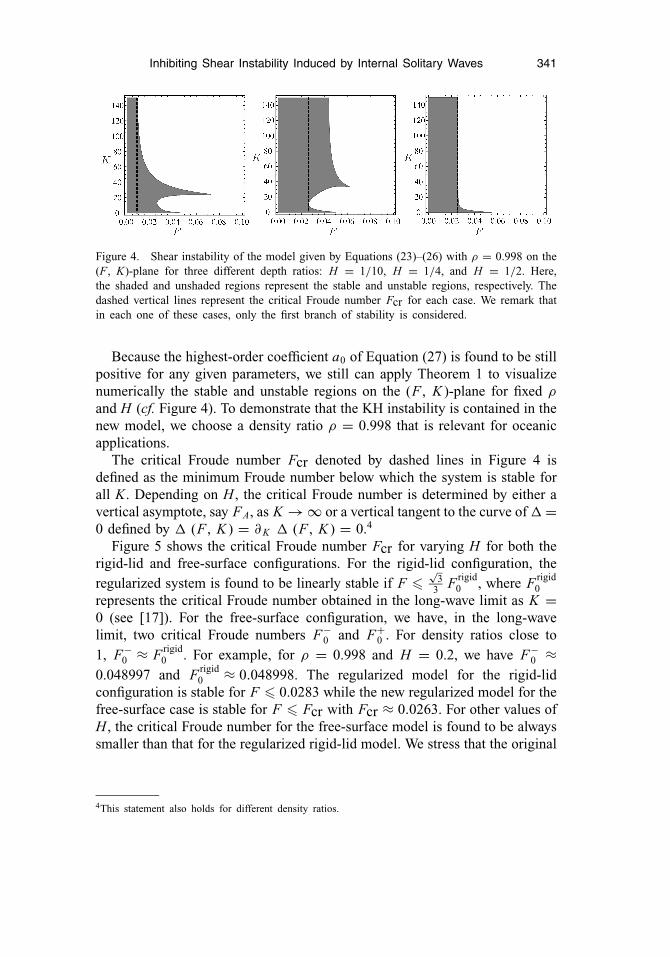
Figure 4. Shear instability of the model given by Equations (23)–(26) with ρ = 0.998 on the(F, K)-plane for three different depth ratios: H = 1/10, H = 1/4, and H = 1/2. Here,the shaded and unshaded regions represent the stable and unstable regions, respectively. Thedashed vertical lines represent the critical Froude number Fcr for each case. We remark thatin each one of these cases, only the first branch of stability is considered.

Because the highest-order coefficient a0 of Equation (27) is found to be stillpositive for any given parameters, we still can apply Theorem 1 to visualizenumerically the stable and unstable regions on the (F , K )-plane for fixed ρ

and H (cf. Figure 4). To demonstrate that the KH instability is contained in thenew model, we choose a density ratio ρ = 0.998 that is relevant for oceanicapplications.

The critical Froude number Fcr denoted by dashed lines in Figure 4 isdefined as the minimum Froude number below which the system is stable forall K. Depending on H , the critical Froude number is determined by either avertical asymptote, say FA, as K → ∞ or a vertical tangent to the curve of =0 defined by (F , K ) = ∂K (F , K ) = 0.4

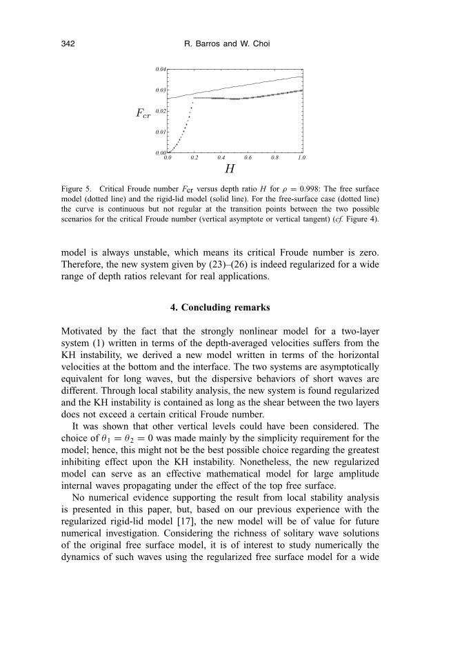
Figure 5 shows the critical Froude number Fcr for varying H for both therigid-lid and free-surface configurations. For the rigid-lid configuration, theregularized system is found to be linearly stable if F �

√3

3 F rigid0 , where F rigid

0represents the critical Froude number obtained in the long-wave limit as K =0 (see [17]). For the free-surface configuration, we have, in the long-wavelimit, two critical Froude numbers F−

0 and F+0 . For density ratios close to

1, F−0 ≈ F rigid

0 . For example, for ρ = 0.998 and H = 0.2, we have F−0 ≈

0.048997 and F rigid0 ≈ 0.048998. The regularized model for the rigid-lid

configuration is stable for F � 0.0283 while the new regularized model for thefree-surface case is stable for F � Fcr with Fcr ≈ 0.0263. For other values ofH , the critical Froude number for the free-surface model is found to be alwayssmaller than that for the regularized rigid-lid model. We stress that the original

4This statement also holds for different density ratios.


Fcr

H0.0 0.2 0.4 0.6 0.8 1.0

0.00

0.01

0.02

0.03

0.04

Figure 5. Critical Froude number Fcr versus depth ratio H for ρ = 0.998: The free surfacemodel (dotted line) and the rigid-lid model (solid line). For the free-surface case (dotted line)the curve is continuous but not regular at the transition points between the two possiblescenarios for the critical Froude number (vertical asymptote or vertical tangent) (cf. Figure 4).

model is always unstable, which means its critical Froude number is zero.Therefore, the new system given by (23)–(26) is indeed regularized for a widerange of depth ratios relevant for real applications.

4. Concluding remarks

Motivated by the fact that the strongly nonlinear model for a two-layersystem (1) written in terms of the depth-averaged velocities suffers from theKH instability, we derived a new model written in terms of the horizontalvelocities at the bottom and the interface. The two systems are asymptoticallyequivalent for long waves, but the dispersive behaviors of short waves aredifferent. Through local stability analysis, the new system is found regularizedand the KH instability is contained as long as the shear between the two layersdoes not exceed a certain critical Froude number.

It was shown that other vertical levels could have been considered. Thechoice of θ1 = θ2 = 0 was made mainly by the simplicity requirement for themodel; hence, this might not be the best possible choice regarding the greatestinhibiting effect upon the KH instability. Nonetheless, the new regularizedmodel can serve as an effective mathematical model for large amplitudeinternal waves propagating under the effect of the top free surface.

No numerical evidence supporting the result from local stability analysisis presented in this paper, but, based on our previous experience with theregularized rigid-lid model [17], the new model will be of value for futurenumerical investigation. Considering the richness of solitary wave solutionsof the original free surface model, it is of interest to study numerically thedynamics of such waves using the regularized free surface model for a wide


range of physical parameters, including front wave solutions of the maximumwave amplitude.

For the rigid-lid case, the Froude number induced by a solitary wave atthe maximal interfacial displacement can be related analytically to the waveamplitude. Therefore, it can be stated that, when the regularized stronglynonlinear model is used, internal solitary waves are stable to perturbationsof arbitrary wavelengths if the wave amplitudes are smaller than a criticalvalue. It would be interesting to obtain an analogous result for the free surfacecase, but no analytic relationship between the Froude number and the waveamplitude has been found yet.

Acknowledgments

The authors gratefully acknowledge support from NSF through GrantDMS-0620832 and ONR through Grant N00014-08-1-0377.

Appendix A: Linear Dispersion for the Original Strongly Nonlinear Model

The linear dispersion relation for the original model (1) is found in dimensionlessform as:

a0c 4 + a1c 3 + a2c 2 + a3c + a4 = 0,

where the expressions for the coefficients are the following:

a0 = (3ρH + 4)H 2 K 4 + 12(H 2 + 3ρH + 1)K 2 + 36,

a1 = −12(F + 1)H (H 2 K 2 + 12)ρK 2 − 8(F + 2)(K 2 + 3)(H 2 K 2 + 3),

a2 = 2[(H 2(9Hρ + 2)K 4 + 6(H 2 + 18ρH + 1)K 2 + 18)F2

+ 6[H 2(3Hρ + 2)K 4 + 6(H 2 + 6ρH + 1)K 2 + 18]F

− 18(−2K 2 + H − 5) + 3H K 2(36ρ + H ((3Hρ + 4)K 2 + 10) − 2)],

a3 = −12H K 2(H 2 K 2 + 12)ρ(F + 1)3 − 8[(K 2 + 3)(H 2 K 2 + 3)F2

+ 3(K 2 + 2)(H 2 K 2 + 3)F + 6K 2+H (2H K 4 + 3(H − 1)K 2 − 9) + 9],

a4 = (F + 1)2 H 2(3Hρ(F + 1)2 + 4)K 4 + 12(3Hρ(F + 1)4

+ F2 + 2F − H + 1)K 2 − 36ρH.

Appendix B: Stability Behavior of the New Regularized System for HighWavenumbers

By considering the limit of K → ∞ along the neutral stability curve given by = 0, we are able to find vertical asymptotes F = FA, as described inSection 3.3.2, as roots of the highest-order coefficient of as a polynomial inthe variable K. This time, these roots are found as roots of a fifth-degree


polynomial P in the variable y = F2:

P(y) = d0 y5 + d1 y4 + d2 y3 + d3 y2 + d4 y + d5,

whose coefficients are given below:

d0 = 96 ρ (3H + 2ρ)3,

d1 = −8[162(2ρ + 1)H 4 + 108(7 − 9ρ)ρH 3 + 9ρ2(13ρ + 96)H 2

+ 12(28 − 27ρ)ρ3 H + 4(8 − 11ρ)ρ4],

d2 = 4H [164ρ5 − 2(79H + 146)ρ4 + 4(H (279H − 190) + 32)ρ3

− 9H (H (155H + 59) − 80)ρ2 + 108(H − 5)(H − 2)H 2ρ

+ 432H 3(H + 1)],

d3 = H 2[48(7ρ − 18)H 4 − 72(ρ(23ρ − 64) + 8)H 3 + 12(ρ(ρ(167ρ − 364)

+ 140) − 72)H 2 + ρ(ρ((644 − 505ρ)ρ + 1352) − 1248)H

+ 24(ρ − 1)2ρ2(19ρ − 16)],

d4 = −4H 3[12(3ρ − 4)H 4 + ((148 − 193ρ)ρ + 48)H 3 − (ρ − 1)(49(ρ − 4)ρ

+ 48)H 2 − (ρ − 1)2(ρ(47ρ + 4) + 48)H − (ρ − 1)3ρ(35ρ − 32)],

d5 = 16H 4(ρ − 1)(H + ρ − 1)4.

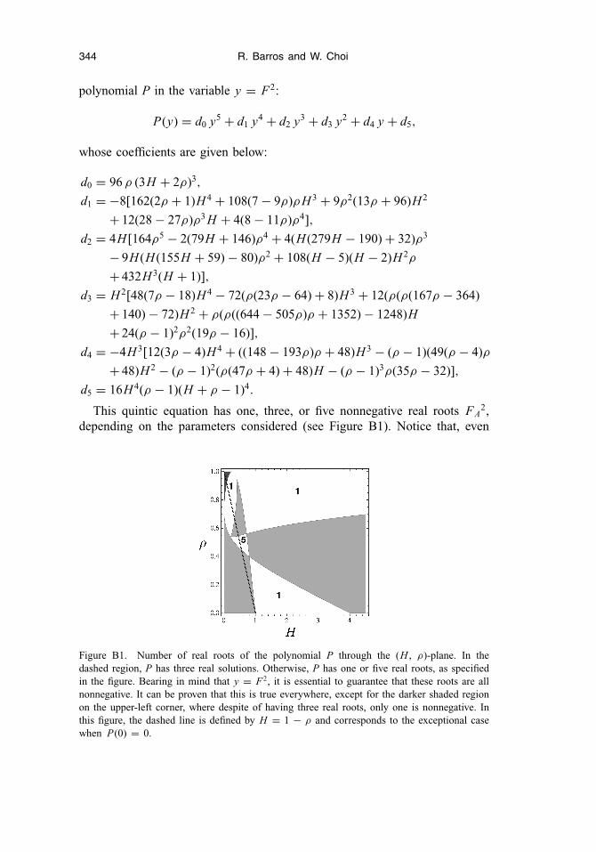
This quintic equation has one, three, or five nonnegative real roots FA2,

depending on the parameters considered (see Figure B1). Notice that, even

Figure B1. Number of real roots of the polynomial P through the (H , ρ)-plane. In thedashed region, P has three real solutions. Otherwise, P has one or five real roots, as specifiedin the figure. Bearing in mind that y = F2, it is essential to guarantee that these roots are allnonnegative. It can be proven that this is true everywhere, except for the darker shaded regionon the upper-left corner, where despite of having three real roots, only one is nonnegative. Inthis figure, the dashed line is defined by H = 1 − ρ and corresponds to the exceptional casewhen P(0) = 0.


if these values do not have to lead to the critical Froude number Fcr (seeFigure 4), these are still candidates for Fcr.

Additionally, given fixed parameter values ρ and H , if all the roots FA arepositive, this implies that the new derived model is able to contain the KHinstability up to a certain critical Froude number Fcr > 0, less or equal to theminimum of these roots FA.

Finally, we remark that this feature cannot be achieved for every parametervalues since, for H = 1 − ρ, we have d5 = 0 or, equivalently, P(0) = 0.

References

1. M. MIYATA, Long internal waves of large amplitude, in Proceedings of the IUTAMSymposium on Nonlinear Water Waves (H. Horikawa and H. Maruo, Eds.), pp. 399–406,1988.

2. W. CHOI and R. CAMASSA, Fully nonlinear internal waves in a two-fluid system, J. FluidMech. 396:1–36 (1999).

3. R. CAMASSA, W. CHOI, H. MICHALLET, P. RUSAS, and J. K. SVEEN, On the realm of validityof strongly nonlinear asymptotic approximations for internal waves, J. Fluid Mech.549:1–23 (2006).

4. J. GRUE, A. JENSEN, P. E. RUSAS, and J. K. SVEEN, Properties of large-amplitude internalwaves, J. Fluid Mech. 380:257–278 (1999).

5. H. MICHALLET and E. BARTHELEMY, Experimental study of interfacial solitary waves, J.Fluid Mech. 366:159–177 (1998).

6. H. MICHALLET and F. DIAS, Numerical study of generalized interfacial solitary waves,Phys. Fluids 11:1502–1511 (1999).

7. F. DIAS and A. IL’ICHEV, Interfacial waves with free-surface boundary conditions: Anapproach via a model equation, Phys. D 150:278–300 (2001).

8. R. BARROS and S. L. GAVRILYUK, Dispersive nonlinear waves in two-layer flows with freesurface. II. Large amplitude solitary waves embedded into the continuous spectrum,Stud. Appl. Math. 119:213–251 (2007).

9. R. BARROS and W. CHOI, On the hyperbolicity of two-layer flows, in Proceedings of the2008 Conference on FACM’08 held at New Jersey Institute of Technology, USA, 19–21May 2008.

10. W. CHOI and R. CAMASSA, Weakly nonlinear internal waves in a two-fluid system, J.Fluid Mech. 313:83–103 (1996).

11. R. BARROS, S. L. GAVRILYUK, and V. M. TESHUKOV, Dispersive nonlinear waves intwo-layer flows with free surface. Part I. Model derivation and general properties, Stud.Appl. Math. 119:191–211 (2007).

12. C. H. SU and C. S. GARDNER, Korteweg-de Vries Equation and Generalizations. Part III.Derivation of the Korteweg-de Vries Equation and Burgers Equation, J. Math. Phys.10:536–539 (1969).

13. A. E. GREEN and P. M. NAGHDI, A derivation of equations for wave propagation in waterof variable depth, J. Fluid Mech. 78:237–246 (1976).

14. R. LISKA, L. MARGOLIN, and B. WENDROFF, Nonhydrostatic two-layer models ofincompressible flow, Comput. Math. Appl. 29:25–37 (1995).


15. T.-C. JO and W. CHOI, Dynamics of strongly nonlinear solitary waves in shallow water,Stud. Appl. Math. 109:205–227 (2002).

16. T.-C. JO and W. CHOI, On stabilizing the strongly nonlinear internal wave model, Stud.Appl. Math. 120:65–85 (2008).

17. W. CHOI, R. BARROS, and T.-C. JO, A regularized model for strongly nonlinear internalsolitary waves, J. Fluid Mech. (2008), in press.

18. H. Y. NGUYEN and F. DIAS, A Boussinesq system for two-way propagation of interfacialwaves, Phys. D 237:2365–2389 (2009).

19. E. I. JURY and M. MANSOUR, Positivity and nonnegativity conditions of a quartic equationand related problems, IEEE Trans. Automat. Contr. AC-26:444–451 (1981).

20. A. T. FULLER, Root location criteria for quartic equations, IEEE Trans. Automat. Contr.AC-26:777–782 (1981).

21. L. V. OVSYANNIKOV, Two-layer “shallow water” model, J. Appl. Mech. Tech. Phys.20:127–135 (1979).

NEW JERSEY INSTITUTE OF TECHNOLOGY

(Received December 10, 2008)

Documents

Inhibiting Shear Instability Induced by Large …wychoi/pub/SAPM_09_2.pdfInhibiting Shear Instability Induced by Large Amplitude Internal Solitary Waves in Two-Layer Flows with a Free