Embed Size (px)
Citation preview

Ranking Routes in Semi-conductor Wafer Fabs
Shreya Gupta
John J. Hasenbein
November 16, 2016
Operations Research and Industrial Engineering
The University of Texas at Austin

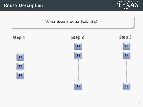
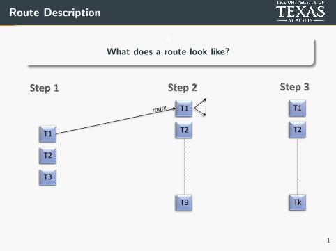
Route Description
a
What does a route look like?
1

Route Description
a
What does a route look like?
T1
T2
T3
T1
T2
T9
T1
T2
Tk
Tool 1
Tool 2
Tool 3
1

Route Description
a
What does a route look like?
T1
T2
T3
T1
T2
T9
1
Route Description
a
What does a route look like?
T1
T2
T3
T1
T2
T9
T1
T2
Tk
1

Route Description
a
What does a route look like?
T1
T2
T3
T1
T2
T9
T1
T2
Tk
1

Route Description
a
What does a route look like?
T1
T2
T3
T1
T2
T9
T1
T2
Tk
1

Route Description
a
What does a route look like?
T1
T2
T3
T1
T2
T9
T1
T2
Tk
1
Route Description
a
What does a route look like?
T1
T2
T3
T1
T2
T9
T1
T2
Tk
1

Route Description
a
What does a route look like?
T1
T2
T3
T1
T2
T9
T1
T2
Tk
1

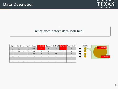
Data Description
a
What does defect data look like?
2

Data Description
a
What does defect data look like?
Step 1 Step 2 … Step N Route Defect 1 Defect 2 Defect 3 Defect 4 Total Defects
T1,1 T2,1 … TN,3 route 1 0 4 53 2 59
T1,2 T2,4 … TN,3 route 2 0 0 0 0 0
T1,3 T2,1 TN,7 route 3 19 2 0 0 21
. . . . . . . . .
. . . . . . . . .
. . … . . . . . . .
Series of steps = Routes
2

Data Description
a
What does defect data look like?
Step 1 Step 2 … Step N Route Defect 1 Defect 2 Defect 3 Defect 4 Total Defects
T1,1 T2,1 … TN,3 route 1 0 4 53 2 59
T1,2 T2,4 … TN,3 route 2 0 0 0 0 0
T1,3 T2,1 TN,7 route 3 19 2 0 0 21
. . . . . . . . .
. . . . . . . . .
. . … . . . . . . .
WafersSeries of steps = Routes
2

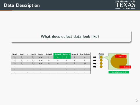
Data Description
a
What does defect data look like?
Step 1 Step 2 … Step N Route Defect 1 Defect 2 Defect 3 Defect 4 Total Defects
T1,1 T2,1 … TN,3 route 1 2 0 0 2 4
T1,2 T2,4 … TN,3 route 2 0 0 0 0 0
T1,3 T2,1 TN,7 route 3 0 4 53 2 59
. . . . . . . . .
. . . . . . . . .
. . … . . . . . . .
Wafers
2
Data Description
a
What does defect data look like?
Defect 4
Defect 1Step 1 Step 2 … Step N Route Defect 1 Defect 2 Defect 3 Defect 4 Total Defects
T1,1 T2,1 … TN,3 route 1 2 0 0 2 4
T1,2 T2,4 … TN,3 route 2 0 0 0 0 0
T1,3 T2,1 TN,7 route 3 0 4 53 2 59
. . . . . . . . .
. . . . . . . . .
. . … . . . . . . .
Wafers
Zero Defects - 2, 3
2

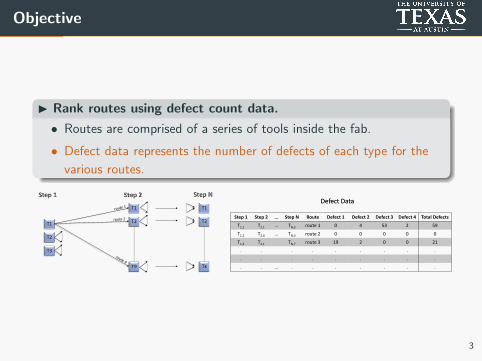
Objective
I Rank routes using defect count data.
• Routes are comprised of a series of tools inside the fab.
• Defect data represents the number of defects of each type for the
various routes.
T1
T2
T3
T1
T2
T9
T1
T2
Tk
Defect Data
Step 1 Step 2 … Step N Route Defect 1 Defect 2 Defect 3 Defect 4 Total Defects
T1,1 T2,1 … TN,3 route 1 0 4 53 2 59
T1,2 T2,4 … TN,3 route 2 0 0 0 0 0
T1,3 T2,1 TN,7 route 3 19 2 0 0 21
. . . . . . . . .
. . . . . . . . .
. . … . . . . . . .
3
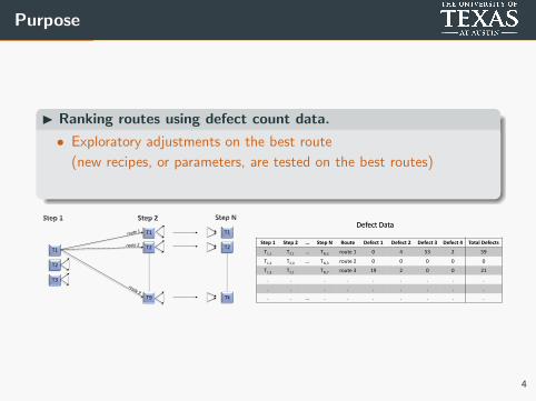
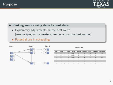
Purpose
I Ranking routes using defect count data.
• Exploratory adjustments on the best route
(new recipes, or parameters, are tested on the best routes)
• Potential use in scheduling
T1
T2
T3
T1
T2
T9
T1
T2
Tk
Defect Data
Step 1 Step 2 … Step N Route Defect 1 Defect 2 Defect 3 Defect 4 Total Defects
T1,1 T2,1 … TN,3 route 1 0 4 53 2 59
T1,2 T2,4 … TN,3 route 2 0 0 0 0 0
T1,3 T2,1 TN,7 route 3 19 2 0 0 21
. . . . . . . . .
. . . . . . . . .
. . … . . . . . . .
4

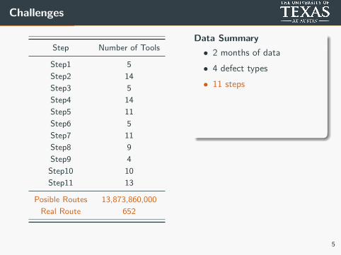
Challenges

Challenges
text
text
March 1, 2016 - April 19, 2016
Data Summary
• 2 months of data
• 4 defect types
• 11 steps
• ≈ 14 billion possible routes
• 652 routes represented
• More than 85% zero defects
5

Challenges
text
text
text
Defects 1, 2, 3, 4
Data Summary
• 2 months of data
• 4 defect types
• 11 steps
• ≈ 14 billion possible routes
• 652 routes represented
• More than 85% zero defects
5
Challenges
Step Number of Tools
Step1 5
Step2 14
Step3 5
Step4 14
Step5 11
Step6 5
Step7 11
Step8 9
Step9 4
Step10 10
Step11 13
Posible Routes 13,873,860,000
Real Route 652
Data Summary
• 2 months of data
• 4 defect types
• 11 steps
• ≈ 14 billion possible routes
• 652 routes represented
• More than 85% zero defects
5

Challenges
Data Summary
• 2 months of data
• 4 defect types
• 11 steps
• ≈ 14 billion possible routes
• 652 routes represented
• More than 85% zero defects
5

Challenges
Objective:
Build a statistical robust heuristic that
can efficiently ranks ≈ 14 Billion routes.
Data Summary
• 2 months of data
• 4 defect types
• 11 steps
• ≈ 14 billion possible routes
• 652 routes represented
• More than 85% zero defects
5

Solution

Model
Step 1 Step 2 … Step N Route Defect 1 Defect 2 Defect 3 Defect 4 Total Defects
T1,1 T2,1 … TN,3 route 1 0 4 53 2 59
T1,2 T2,4 … TN,3 route 2 0 0 0 0 0
T1,3 T2,1 TN,7 route 3 19 2 0 0 21
. . . . . . . . .
. . . . . . . . .
. . … . . . . . . .
WafersSeries of steps = Routes
6

Model
Step 1 Step 2 … Step N Route Defect 1 Defect 2 Defect 3 Defect 4 Total Defects
T1,1 T2,1 … TN,3 route 1 0 4 53 2 59
T1,2 T2,4 … TN,3 route 2 0 0 0 0 0
T1,3 T2,1 TN,7 route 3 19 2 0 0 21
. . . . . . . . .
. . . . . . . . .
. . … . . . . . . .
Counts / Positive Numbers / Positive Integers
Defect 4
Defect 1Wafers
Zero Defects - 2, 3
6

Model
Counts / Positive Numbers / Positive Integers
Step 1 Step 2 … Step N Route Defect 1 Defect 2 Defect 3 Defect 4 Total Defects
T1,1 T2,1 … TN,3 route 1 0 4 53 2 59
T1,2 T2,4 … TN,3 route 2 0 0 0 0 0
T1,3 T2,1 TN,7 route 3 19 2 0 0 21
. . . . . . . . .
. . . . . . . . .
. . … . . . . . . .
Count Regression
6

Model
14 billion routes
Step 1 Step 2 … Step N Route Defect 1 Defect 2 Defect 3 Defect 4 Total Defects
T1,1 T2,1 … TN,3 route 1 2 0 0 2 4
T1,2 T2,4 … TN,3 route 2 0 0 0 0 0
T1,3 T2,1 TN,7 route 3 0 4 53 2 59
. . . . . . . . .
. . . . . . . . .
. . … . . . . . . .
6
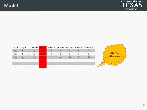
Model
Is there a better way?
Step 1 Step 2 … Step N Route Defect 1 Defect 2 Defect 3 Defect 4 Total Defects
T1,1 T2,1 … TN,3 route 1 2 0 0 2 4
T1,2 T2,4 … TN,3 route 2 0 0 0 0 0
T1,3 T2,1 TN,7 route 3 0 4 53 2 59
. . . . . . . . .
. . . . . . . . .
. . … . . . . . . .
6

Model
Step 1 Step 2 … Step N Route Defect 1 Defect 2 Defect 3 Defect 4 Total Defects
T1,1 T2,1 … TN,3 route 1 2 0 0 2 4
T1,2 T2,4 … TN,3 route 2 0 0 0 0 0
T1,3 T2,1 TN,7 route 3 0 4 53 2 59
. . . . . . . . .
. . . . . . . . .
. . … . . . . . . .
Count Regression
6

Model
Step 1 Step 2 … Step N Route Defect 1 Defect 2 Defect 3 Defect 4 Total Defects
T1,1 T2,1 … TN,3 route 1 2 0 0 2 4
T1,2 T2,4 … TN,3 route 2 0 0 0 0 0
T1,3 T2,1 TN,7 route 3 0 4 53 2 59
. . . . . . . . .
. . . . . . . . .
. . … . . . . . . .
Count Regression
6

Model
Step 1 Step 2 … Step N Route Defect 1 Defect 2 Defect 3 Defect 4 Total Defects
T1,1 T2,1 … TN,3 route 1 2 0 0 2 4
T1,2 T2,4 … TN,3 route 2 0 0 0 0 0
T1,3 T2,1 TN,7 route 3 0 4 53 2 59
. . . . . . . . .
. . . . . . . . .
. . … . . . . . . .
Count Regression
6

Model
Step 1 Step 2 … Step N Route Defect 1 Defect 2 Defect 3 Defect 4 Total Defects
T1,1 T2,1 … TN,3 route 1 2 0 0 2 4
T1,2 T2,4 … TN,3 route 2 0 0 0 0 0
T1,3 T2,1 TN,7 route 3 0 4 53 2 59
. . . . . . . . .
. . . . . . . . .
. . … . . . . . . .
Count Regression
6

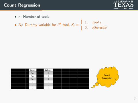
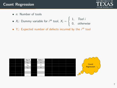
Count Regression
• n: Number of tools
• Xi : Dummy variable for i th tool, Xi =
{1, Tool i
0, otherwise
• Yi : Expected number of defects incurred by the i th tool
• log(Yi ) = β1 +n∑
i=2
βiXi
• Yi =
{eβ1 , Tool i = 1
eβ1+βi , Tool i 6= 1
Step 1 Step 2 … Step N Route Defect 1 Defect 2 Defect 3 Defect 4 Total Defects
T1,1 T2,1 … TN,3 route 1 2 0 0 2 4
T1,2 T2,4 … TN,3 route 2 0 0 0 0 0
T1,3 T2,1 TN,7 route 3 0 4 53 2 59
. . . . . . . . .
. . . . . . . . .
. . … . . . . . . .
Count Regression
7
Count Regression
• n: Number of tools
• Xi : Dummy variable for i th tool, Xi =
{1, Tool i
0, otherwise
• Yi : Expected number of defects incurred by the i th tool
• log(Yi ) = β1 +n∑
i=2
βiXi
• Yi =
{eβ1 , Tool i = 1
eβ1+βi , Tool i 6= 1
Step 1 Step 2 … Step N Route Defect 1 Defect 2 Defect 3 Defect 4 Total Defects
T1,1 T2,1 … TN,3 route 1 2 0 0 2 4
T1,2 T2,4 … TN,3 route 2 0 0 0 0 0
T1,3 T2,1 TN,7 route 3 0 4 53 2 59
. . . . . . . . .
. . . . . . . . .
. . … . . . . . . .
Count Regression
7

Count Regression
Our Approach
We begin modeling the defect count data set from the most basic and
proceed forward until we find the model that best fits our data.
8

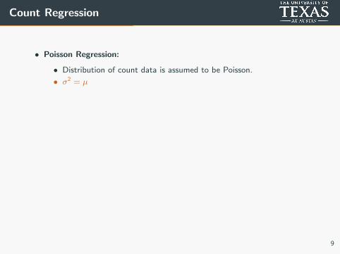
Count Regression
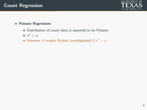
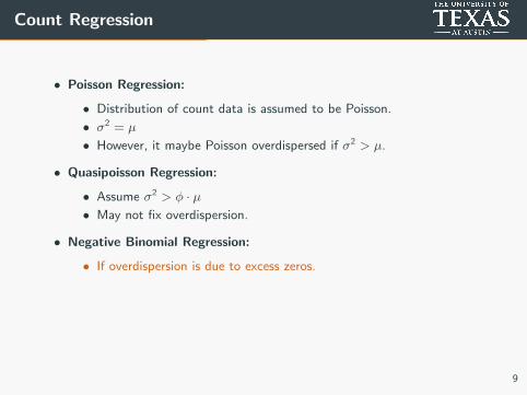
• Poisson Regression:
• Distribution of count data is assumed to be Poisson.
• σ2 = µ
• However, it maybe Poisson overdispersed if σ2 > µ.
• Quasipoisson Regression:
• Assume σ2 > φ · µ• May not fix overdispersion.
• Negative Binomial Regression:
• If overdispersion is due to excess zeros.
• Negative Binomial accounts for excess zeros well.
• Negative Binomial overdispersion or a bad fit may occur due to
excess zeros beyond what the NB fit can account for.
9

Count Regression
• Poisson Regression:
• Distribution of count data is assumed to be Poisson.
• σ2 = µ
• However, it maybe Poisson overdispersed if σ2 > µ.
• Quasipoisson Regression:
• Assume σ2 > φ · µ• May not fix overdispersion.
• Negative Binomial Regression:
• If overdispersion is due to excess zeros.
• Negative Binomial accounts for excess zeros well.
• Negative Binomial overdispersion or a bad fit may occur due to
excess zeros beyond what the NB fit can account for.
9

Count Regression
• Poisson Regression:
• Distribution of count data is assumed to be Poisson.
• σ2 = µ
• However, it maybe Poisson overdispersed if σ2 > µ.
• Quasipoisson Regression:
• Assume σ2 > φ · µ
• May not fix overdispersion.
• Negative Binomial Regression:
• If overdispersion is due to excess zeros.
• Negative Binomial accounts for excess zeros well.
• Negative Binomial overdispersion or a bad fit may occur due to
excess zeros beyond what the NB fit can account for.
9

Count Regression
• Poisson Regression:
• Distribution of count data is assumed to be Poisson.
• σ2 = µ
• However, it maybe Poisson overdispersed if σ2 > µ.
• Quasipoisson Regression:
• Assume σ2 > φ · µ• May not fix overdispersion.
• Negative Binomial Regression:
• If overdispersion is due to excess zeros.
• Negative Binomial accounts for excess zeros well.
• Negative Binomial overdispersion or a bad fit may occur due to
excess zeros beyond what the NB fit can account for.
9

Count Regression
• Poisson Regression:
• Distribution of count data is assumed to be Poisson.
• σ2 = µ
• However, it maybe Poisson overdispersed if σ2 > µ.
• Quasipoisson Regression:
• Assume σ2 > φ · µ• May not fix overdispersion.
• Negative Binomial Regression:
• If overdispersion is due to excess zeros.
• Negative Binomial accounts for excess zeros well.
• Negative Binomial overdispersion or a bad fit may occur due to
excess zeros beyond what the NB fit can account for.
9

Count Regression
• Hurdle Model:
• Hierarchical approach.
• Level 1:
Treat count data as a Bernoulli process with p being the probability
of incurring a defect and 1− p the probability of zero defects.
• Level 2: In the case of positive defects, the positive defect counts
are modeled as a zero-truncated count process.
• Expected defect count, E [Yi ] =
{p1 · eβ1 , Tool i = 1
pi · eβ1+βi , Tool i 6= 1
10

Count Regression
• Hurdle Model:
• Hierarchical approach.
• Level 1:
Treat count data as a Bernoulli process with p being the probability
of incurring a defect and 1− p the probability of zero defects.
• Level 2: In the case of positive defects, the positive defect counts
are modeled as a zero-truncated count process.
• Expected defect count, E [Yi ] =
{p1 · eβ1 , Tool i = 1
pi · eβ1+βi , Tool i 6= 1
Count Data
Zero Defect
Defect Count > 0
Zero-truncated Poisson counts
Zero-truncated NB counts
1-p
p
10

Count Regression Models
Snapshot: Best Count Model Fit
Defect Step Regression Type P-value Dispersion AIC Best Fit
def1 Step1 Poisson 0.00 3.73 6577.11 No
def1 Step1 Quasipoisson 0.00 3.73 1e+07 No
def1 Step1 Negative Binomial 0.02 1.09 5029.06 No
def1 Step1 Hurdle - Poisson NA NA 6312.13 No
def1 Step1 Hurdle - Negative Binomial NA NA 5012.51 Yes
def2 Step3 Poisson 0.00 2.52 6525.1 No
def2 Step3 Quasipoisson 0.00 2.52 1e+07 No
def2 Step3 Negative Binomial 1.00 0.77 5026.4 No*
def2 Step3 Hurdle - Poisson NA NA 6293.64 No
def2 Step3 Hurdle - Negative Binomial NA NA 5017.27 Yes
* This model was not considered a best fit in spite of having a significant p-value
> α(= 0.5) because the dispersion was 6≈ 1.25. Also, another model (Hurdle - Negative
Binomial) yielded a lower AIC statistic.
NA: Could not be extracted using R or model does not have this statistic
11

Ranking Algorithm
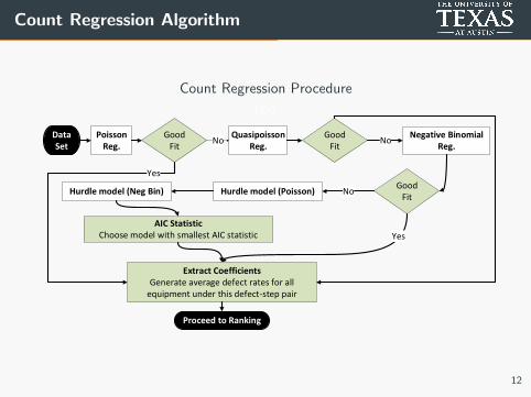
Count Regression Algorithm
Count Regression Procedure
text
Poisson Reg.
GoodFit
Yes
Quasipoisson Reg.
NoNegative Binomial
Reg.
Yes
Hurdle model (Poisson)Hurdle model (Neg Bin)
Extract CoefficientsGenerate average defect rates for all
equipment under this defect-step pair
GoodFit
No
GoodFit
No
Data Set
Proceed to Ranking
AIC StatisticChoose model with smallest AIC statistic
12

Ranking Algorithm
Snapshot: Defect-1 Tool Ranks
Defect Step Tools (i) Model Yi Rank
def1 Step1 EQP 31 Hurdle - NB 23.21 5
def1 Step1 EQP 32 Hurdle - NB 3.42 3
def1 Step1 EQP 35 Hurdle - NB 2.71 1
def1 Step1 EQP 36 Hurdle - NB 3.03 2
def1 Step11 EQP 60 Hurdle - NB 2.80 4
def1 Step11 EQP 61 Hurdle - NB 2.87 5
def1 Step11 EQP 62 Hurdle - NB 3.59 11
def1 Step11 EQP 50 Hurdle - NB 23.96 12
Step 1: Tool Ranks
Assign ranks from 1 to n to the tools under this step.
- Highest rank, 1, for the tool generating the smallest number of defects.
- Lowest rank, n, for the tool generating the largest number of defects.
13
Ranking Algorithm
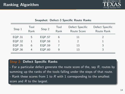
Snapshot: Defect-3 Specific Route Ranks
Step 1Tool
RankStep 2
Tool
Rank
Defect Specific
Route Score
Defect Specific
Route Rank
EQP 31 5 EQP 57 6 11 2
EQP 32 1 EQP 58 1 2 1
EQP 35 6 EQP 59 7 13 3
EQP 36 4 EQP 60 9 13 3
Step 2: Defect Specific Ranks
- For a particular defect generate the route score of the, say R, routes by
summing up the ranks of the tools falling under the steps of that route.
- Rank these scores from 1 to R with 1 corresponding to the smallest
score and R to the largest.
14
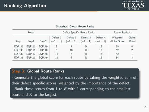
Ranking Algorithm
Snapshot: Global Route Ranks
Route Defect Specific Route Ranks Route Statistics
Step1 Step2 Step3
Defect 1
(w1 = 1)
Defect 2
(w2 = 1)
Defect 3
(w3 = 1)
Defect 4
(w4 = 1)
Weighted
Global Score
Global
Rank
EQP 35 EQP 16 EQP 49 8 5 24 18 55 4
EQP 38 EQP 16 EQP 48 6 10 19 17 52 2
EQP 32 EQP 10 EQP 48 14 7 8 13 42 1
EQP 31 EQP 16 EQP 49 12 6 21 15 54 3
Step 3: Global Route Ranks
- Generate the global score for each route by taking the weighted sum of
their defect specific scores, weighted by the importance of the defect.
- Rank these scores from 1 to R with 1 corresponding to the smallest
score and R to the largest.
15

Conclusions

Future Work
1. The methodology could be incorporated into scheduling
algorithms.
2. Statistically significant differences between routes may be
evaluated.
3. Validation against out-of-sample data.
16

Future Work
1. The methodology could be incorporated into scheduling
algorithms.
2. Statistically significant differences between routes may be
evaluated.
3. Validation against out-of-sample data.
16
Future Work
1. The methodology could be incorporated into scheduling
algorithms.
2. Statistically significant differences between routes may be
evaluated.
3. Validation against out-of-sample data.
16

Additional Work
I Score-based Ranking
For output data like yield (greater the better), we have developed a
ranking technique using ANCOVA and Tukey HSD pair-wise difference
techniques that rank routes based on the significant differences between
their output levels.
17

Additional Work
(ii) Target-based Ranking
For output metrics like thickness, which have upper and lower
specifications bounding the target to be achieved, we have designed
ranking techniques that rank routes based on the accuracy and precision
of their output.
18

Questions
19

Thank You

Appendix
Appendix 1
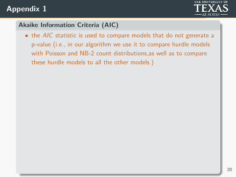
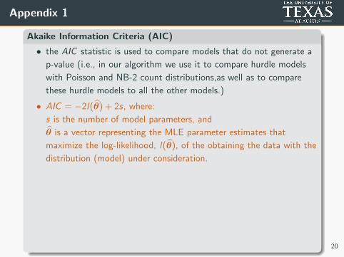
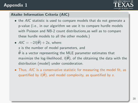
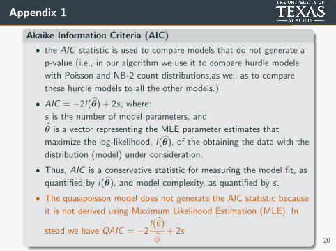
Akaike Information Criteria (AIC)
• the AIC statistic is used to compare models that do not generate a
p-value (i.e., in our algorithm we use it to compare hurdle models
with Poisson and NB-2 count distributions,as well as to compare
these hurdle models to all the other models.)
• AIC = −2l(θ̂) + 2s, where:
s is the number of model parameters, and
θ̂ is a vector representing the MLE parameter estimates that
maximize the log-likelihood, l(θ̂), of the obtaining the data with the
distribution (model) under consideration.
• Thus, AIC is a conservative statistic for measuring the model fit, as
quantified by l(θ̂), and model complexity, as quantified by s.
• The quasipoisson model does not generate the AIC statistic because
it is not derived using Maximum Likelihood Estimation (MLE). In
stead we have QAIC = −2l(θ̂)
φ̂+ 2s
20
Appendix 1
Akaike Information Criteria (AIC)
• the AIC statistic is used to compare models that do not generate a
p-value (i.e., in our algorithm we use it to compare hurdle models
with Poisson and NB-2 count distributions,as well as to compare
these hurdle models to all the other models.)
• AIC = −2l(θ̂) + 2s, where:
s is the number of model parameters, and
θ̂ is a vector representing the MLE parameter estimates that
maximize the log-likelihood, l(θ̂), of the obtaining the data with the
distribution (model) under consideration.
• Thus, AIC is a conservative statistic for measuring the model fit, as
quantified by l(θ̂), and model complexity, as quantified by s.
• The quasipoisson model does not generate the AIC statistic because
it is not derived using Maximum Likelihood Estimation (MLE). In
stead we have QAIC = −2l(θ̂)
φ̂+ 2s
20

Appendix 2
Bayesian Information Criterion (BIC)
• BIC is analogous to AIC except 2s is replaced with s log n. BIC
imposes a stronger penalty on model complexity than AIC for
n ≥ 8,i.e., when sample size is large (Zheng and Loh 1995).
• So, BIC = −2l(θ̂) + s log n
• See Burnham and Anderson 2002 for all variants of AIC.
21
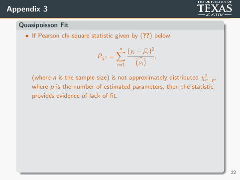
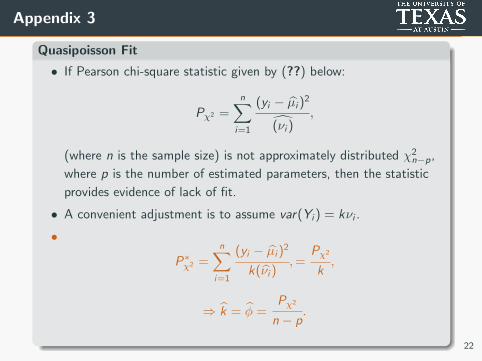
Appendix 3
Quasipoisson Fit
• If Pearson chi-square statistic given by (??) below:
Pχ2 =n∑
i=1
(yi − µ̂i )2
(̂νi ),
(where n is the sample size) is not approximately distributed χ2n−p,
where p is the number of estimated parameters, then the statistic
provides evidence of lack of fit.
• A convenient adjustment is to assume var(Yi ) = kνi .
•
P∗χ2 =n∑
i=1
(yi − µ̂i )2
k(ν̂i ),=
Pχ2
k,
⇒ k̂ = φ̂ =Pχ2
n − p.
22

Appendix 3
Quasipoisson Fit
• The exponential family f (y ;ψ, φ̂) (where ψ is the mean) may no
longer integrate to unity and is should be simply considered a useful
modification of the likelihood function.
• Only the variance changes with an adjustment factor of k estimated
by φ̂ and this is accounted for by:
∂l ′(β; y)
∂βj= 0) j = 1, . . . , p;
⇒1
φ̂
n∑i=1
∂µi
∂βj(yi − µi )
νi=
1
φ̂
(∂l(β; y)
∂βj
)j = 1, . . . , p.
• Thus, the MLE estimates remain unchanged.
23
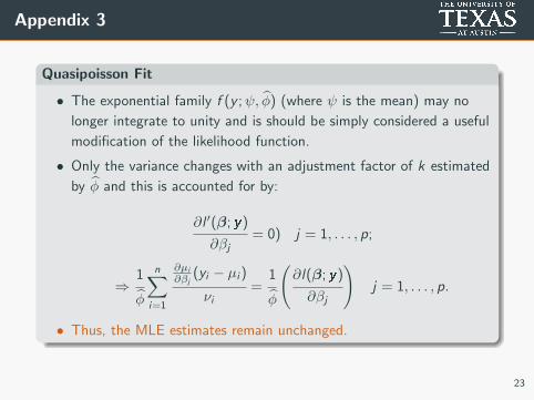


