Information capacity of associative memories

IEEE TRANSACTIONS ON INFORMATION THEORY, VOL. 35, NO. 1, JANUARY 1989 59

Information Capacity of Associative Memories

Abstract -Associative memory networks, consisting of highly interconnected binary-valued cells, have been used to model neural networks. Tight asymptotic bounds have been found for the information capacity of these networks. We derive the asymptotic information capacity of these networks using results from normal approximation theory and theorems about exchangeable random variables.

I. INTRODUCTION

OR MANY YEARS researchers in various disciplines F have studied models for the brain. Many models have been developed in attempts to understand how neural networks function. One class of such models is based on the concept of associative memory [1]-[27]. Associative memories are composed of a collection of interconnected elements having data storage capabilities. The elements are accessed in parallel by a data probe vector rather than by a set of specific addresses [14].

Recent years have seen interest increasing in the model- ing of neural networks for possible applications to computer architectures. Associative memory network (AMN) models of one particular form, consisting of highly interconnected threshold devices [l], [2], [5]-[12], [24]-[27] have received much attention. These models are sometimes referred to as binary associative memory networks (BAMN’s).

This paper discusses some analytical aspects of the BAMN models. Specifically, we analyze the storage capabilities of these models. We consider the case where cells can take on only one of two values { - l,l}. Our work is motivated by a desire to understand better the results of [12], where various elaborate arguments are used to find the asymptotic value of the network storage capacity. In contrast, we determine the asymptotic network storage capacity by applying normal approximation theory and theorems about exchangeable random variables. This new approach contributes to a better understanding of the results and provides a means of extending the analysis to more general AMN models.

Manuscript received January 26, 1988; revised April 13, 1988. T h s work was supported in part by the Office of Naval Research under Grant N00014-83-K-0577, in part by the National Science Foundation under Grants ECS84-05460 and MIP-8710868, and in part by the Pacific International Center for High Technology Research. This work was partially presented at the 1986 IEEE International Symposium on Infor- mation Theory, Ann Arbor, MI.

A. Kuh is with the Department of Electrical Engineering, University of Hawaii at Manoa, Honolulu, HI 96822.

B. W. Dickinson is with the Department of Electrical Engineering, Princeton University, Princeton, NJ 08544.

IEEE Log Number 8825711.

In Section I1 the standard BAMN model and the notion of capacity of the network are described. The operation and the construction of the standard model are discussed. In this model each updating operation on a cell is performed by thresholding a linearly weighted sum of other cell values. If the threshold is exceeded the cell takes on a 1 value; otherwise, it takes on a -1 value. A network is characterized by a matrix of weights that determines the strengths of the interconnections between different cells. The weight matrix is constructed from a sum of outer products of vectors chosen to be the desired “codewords” to be stored by the network.

The information capacity of the standard model is derived in Section 111. This requires a formalization of the notions of capacity and stability. Following [12] we consider two different definitions. In the first, capacity is related to the maximum number of codewords that can be used to construct the AMN while maintaining a fixed codeword as a stable vector. In the second definition, the capacity is related to the largest number of codewords that can all be stored as stable vectors in the network. We also consider the radius of attraction of each of these codewords. For example, if the state of the AMN after a few update operations converges to a given vector for all initial probe vectors at a Hamming distance of K or less, then the gven stable vector has a radius of attraction of at least K. Proofs of the various results are given in the Appendices. They involve normal approximation theory and theorems from exchangeable random variables. Finally, in Section IV we summarize the main theoretical results of this paper and introduce extensions for further research.

11. OPERATION AND CONSTRUCTION OF THE BINARY ASSOCIATIVE MEMORY NETWORK MODEL

In this section we discuss the AMN model presented in [ 11, [2], sometimes referred to as the binary associative memory network. A network consists of cells { X , } , 12 i 5 N , with each cell taking on one of the values { - 1,1}. Each cell affects all other cells through an interconnection or weight matrix T. The interconnection matrix is symmetric with 0 values on its diagonal. Each cell is updated at random with the update events forming a Poisson process with rate A. At each update the linearly weighted sum of all other cell values is compared to a given threshold. If the weighted sum exceeds the threshold, the cell takes on a 1 value; if not, the cell takes on a - 1 value. We assume that the updating processes of all cells are independent, so that the total number of updates is a Poisson process with rate

0018-9448/89/0100-0059$01.00 01989 IEEE

60 IEEE TRANSACTIONS ON INFORMATION THEORY, VOL. 35, NO. 1, JANUARY 1989

NX. Using a counter k that is incremented every time any cell is updated, an update of cell i at time k +1 is described by the equation

where 1, x > o

p ( x , y ) = Y , x = o . i -1, x < o

Here we have chosen a 0 threshold. For an AMN with interconnection matrix T , we define a

binary N vector V to be invariant if, when V is input into the network, all updates leave the state of the network unchanged. An invariant vector is also called a stable uector of the AMN. The set of all stable vectors is denoted by M .

Now consider the construction of an AMN, a process that can be viewed as learning. The T matrix is constructed so that certain vectors are stored in the network. A vector is successfully stored in the network if it can be retrieved by an appropriate data probe vector. We let V(i), 1 1 i s m be the codewords, binary N vectors, used to construct the T matrfix. The desired behavior of the model when some vector V is input into the network, i.e., when the network is initialized at I/, is that after a few updates, the state of the netyork should become V, a stable vector whch is close to V in Hamming distance. Several techniques can be used to construct the T matrix of the AMN. Here we use a simple technique involving correlation, which contrasts with techniques using eigenvectors and orthogonal learning approaches shown in [14], [18], [24]; the latter are more complicated to implement. The correlation technique constructs the T matrix from { V(i)} as follows. Let

T, = ~ ( i ) ~ ( i ) ~ - I , 1 I i I m (2.2) and then take

m

T = T,, r = l

(2.3)

Hopefully, all of the chosen codewords { V(i)} will be stable vectors of the network; however, this cannot occur when m becomes too large in comparison to N. The set of all codewords that are stable vectors is called M,. Thus M,. c M , but M also contains the “one’s complement” of vectors in M,. and possibly other vectors whch we call spurious stable vectors.

To find the capacity of these networks, random coding arguments are used; each component of each codeword is assumed to be chosen independently of all other compo- nents, with the probability of a 1 or - 1 each equal to 1/2. Then, given m randomly chosen codewords, one can find the probability that any codeword or that all the chosen codewords are members of M . Two definitions for capacity which we call Z(E) and & ( E ) are introduced in [12]. Before presenting these definitions, we define a synchronous update AcV) as a simultaneous uDdate on all N

cells with V initially input into the network. It is easily shown that if V is a stable vector then V = A(V); the converse is not necessarily true. This stronger condition is used in defining Z(E) as

% ( E ) = m a x m 3 P r ( V ( k ) = A ( V ( k ) ) ) > l - c (2.4)

(where we may take k = 1) and &( E ) as

& ( c ) = maxm 3 Pr( V(i) = A ( V(i)), 1 I i I m ) >1- c .

(2.5)

We show in Section I11 that E ( € ) = N/2log N and that & ( E ) = N/4log N for any E > 0 and for N sufficiently large; these results were obtained by different, more te- dious methods in [12].

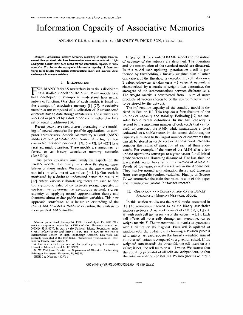
We first present a simple example to help visualize how these AMN models work. Take N = 4 and m = 3, and let

Using the correlation method, T is easily found to be

r o 1 3 -11 I = [ 3 1 0 1 0 1 -‘J.

-1 1 -1 0 We note that only V(3) E M , (i.e., M, = { V(3))). Fig. 1 shows a diagram of this model.

Fig. 1. Example network with edges representing interconnection weights and nodes representing cells.

Before concluding this section we note that in our analysis we always assume that any initial state will converge to a stable vector. This was justified by Hopfield in [2] by noting that

1 E = - - c x T ( i , j ) X , ( k ) X , ( k ) , k 2 0 (2.6)

is a monotonic decreasing function of the update counter k and that the elements of M correspond to the local minima of E . Therefore, any initial state will converge to a stable vector.

2 f J

111. DERIVATION OF THE INFORMATION CAPACITY FOR THE BAMN MODEL

This section studies the capacities Z(c) and & ( E ) using results from normal approximation theory and theorems about exchangeable random variables. Our main results

KUH AND DICKINSON: INFORMATION CAPACITY OF ASSOCIATIVE MEMORIES 61

are asymptotic expressions for these quantities. We discuss the two patterns for convergence of initial states to some stable vector. We also consider the error-correcting capabilities or the radius of attraction of each codeword. Much of the original discussion about capacity, convergence, and radius of attraction can be found in [12] and [24]. The key differences in our approach versus that of [12] are the proofs of the main theorems; these are given in the appendices.

Associated with each cell value we define the interaction strength (IS) of cell j for codeword k as

m

f # j i f j / = I

= ( N - W g k ) + c c Y ( W g O W ) . i f j l f k

( 3 4

According to the standard model, when a cell is updated its next value is determined from a comparison of its IS with a threshold value. Using the random coding model described in the previous section U ( j , k ) is a random variable. We transform this random variable by letting

~ ( j , k ) = C C ~ ( l ) y ( ' ) ~ ( k ) ? ( k ) = C U j ( l > i # j l f k If k

= [U( j , k ) - ( N - 1) v, ( k ) ] v , ( k ) ( 3 4

where we call ~ ( j , k ) the normalized interaction strength (NIS). The u j ( / ) for I # k are random variables having probability mass function identical to a shfted binomial random variable with mean 0, N - 1 points, and parameter p = 1/2. Since V( I ) are chosen independently for all 1, the U( j , k ) are random variables having probability mass function identical to a shifted binomial random variable with mean 0, ( N - l ) ( m -1) points, and parameter p =

1/2. To evaluate Z ( E ) we need to compute

p = Pr( V ( k ) = A ( V ( k ) ) )

= P r n { U ( j , k ) > - N + l } (3.3) i " j = l

(where we may take k =l) . To evaluate hi(€) we need to compute

j = Pr ( V ( k ) = A ( V ( k ) ) , 1 I k I m )

= P r n n { U ( j , k ) > - - N + i } ] [ j I , ,, (3.4)

The major stumbling block to analyzing (3.3) and (3.4) is the fact that the ~ ( j , k ) are not independent. In fact, it is easily shown that

( ( N - l ) ( m - l ) , j = l , k = m j # l , k = m j = l , k # m otherwise.

(3.5)

By the Demoivre-Laplace theorem [28], for large N, U( j , k ) converges in distribution to a Gaussian random variable with the same first- and second-order moments. Thus we let g ( j , k ) be a Gaussian random variable with the same first- and second-order moments as U( j , k ) and investigate the quantities

{ g ( j , k ) > - N + I } ] (3.6) j = l

and / N m

j , = P r n n { g ( j , k ) > - N + i } . (3.7) 1 j = l k = l 1 Let Q ( x ) = ( 1 / f i ) j ~ e X z / * dx be the standard normal error function and I ( . ) be the standard indicator function. In Appendix I we develop and use the theory of exchangeable random variables to show the following result.

Theorem I : 1) If N N

and YN is a Poisson random variable with parameter A, = N Q ( \ / N / m ) , then X , + Y, in distribution.

2) If

and Y, is a Poisson random variable with parameter A, = N m Q ( \ / N / m ) , then X N + YN in distribution.

We can use this theorem to evaluate the capacities defined earlier. Letting m = N / a log N we solve for the constant a for both cases. From the theorem, for large N we have

pc = e - ~ ~ ( J N / m ) (3.8)

j , = e-h'mQ(JN/m). (3.9)

and

By repeated integration by parts we obtain the expansion

Hence, for large x, we have the approximation Q ( x ) = e - " ' / , / x G . Then we have the following result.

Theorem 2: For case 1) in Theorem 1, assuming j = pc, pc >> e P N , and as N + 00,

- P , ) N

I I

-1og(logN)-log4~

N 1 .

I

210g N '

( 3 .lo)


For case 2) in Theorem 1, assuming j = j?,, j G >> e-”*, and as N -+ CO,

w - a,> N

410g N - 210g (log [ ) ) - 3 log (log N ) -log 12 th

=

N

41og N ’ s- (3.11)

Next we consider conditions under wluch PG + P and j?, -+ 8. Appendix I1 shows that when N is sufficiently large and m = N/a log N for 1/2 < a << N/log N then pC -+ ji. This is a consequence of normal approximation theory. It can similarly be shown that j?, - a. Therefore, for any c > 0 we can find an N large enough such that K ( c ) = N/2logN and G(c) = N/4logN.

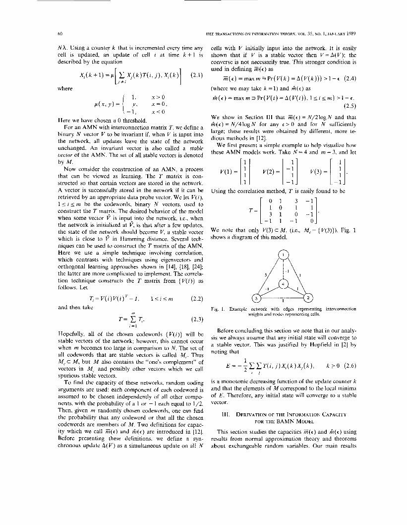
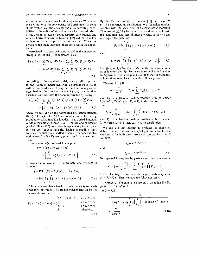
In Fig. 2 we plot some simulation results for p as a function of m/N; we also plot the theoretical graph of Pc versus m/N. For N = 16 the simulations and the Gaussian approximations differ substantially, but for N = 256 the simulations and the Gaussian approximations are almost identical. The simulations were performed by choosing random codewords, updating the T matrix, and then checking if V(1) E M . Tlus process is continued until the number of codewords, m = O( N). This gives a simulation of one sample network and is shown in Fig. 3. From Monte Carlo simulations of several sample networks, the value of for a given m is easily found.

1 .o

0.8

0.6 In U- theory N=16

0.4

0.2

0.0 0 . 0 0 2 0 . 4 0.6 0 . 8 1 .0

miN

Fig. 2. Simulations comparing theoretical Gaussian approximation & to Monte Carlo simulations of p for N = 16, N = 64, and N = 256.

To this point our assumption has been that we input a codeword with no errors and then calculate the probability that the state of the system does not change after any update. In AMN we are also interested in recovering stored patterns even when some information about the data is lost. For a fixed AMN, we say that a cod:word V has K error correcting ability if all vectors V withm Hamming distance K :re correctable by one synchronous update, that is, V = A( V ) . We can then evaluate the capacity of the network if we require all codewords to be K error correcting with high probability or if we require a

T = T + T ,

Fig. 3. Algorithm used for conducting simulations of p

typical codeword to be K error correcting. We define these two capacities as &(c, K ) and Z ( c , K ) , respectively.

Using the same type of arguments as in the first part of this section, we first find the NIS:

u ( j , k , f ) = C C ~ ( i ) y ( i ) t ( k ) q ( k ) = C U,([). r f j I # k I z k

(3.12)

From (3.2), we note that u ( j , k , 8) has the same distribution as u ( j , k ) . Observe that

N - 1 - 2 K = y ( k ) y ( k ) t ( k ) q ( k ) (3.13)

when h(V(k), 8 ( k ) ) = K (where h(x, y ) is the Hamming distance between x and y ) . We then define the quantities

l # J

p ( K ) = P r [ V ( k ) = A ( P ) l h ( V ( k ) , ? ) ‘K)

= P r [ f i { u ( j , k , $ ) > - N + 1 + 2 K } , J = 1 1

1’ k < m (3.14) and

j ? ( K ) = Pr ( V ( k ) = A ( P( k ) ) Ih ( V ( k ) , P( k ) )

- < K , l < k < m )

(3.15)

in analogy to (3.3) and (3.4). By worlung with the corresponding Gaussian quantities pG( K ) and bG( K), Theo- rem A2 and normal approximation theory give the following result.

Theorem 3: Asymptotically, as N -+ 00 and for all K < N/2

( N - 2 K ) ’ Z K ( f ) =

2NlogN (3.16)

KUH AND DICKINSON: INFORMATION CAPACITY OF ASSOCIATIVE MEMORIES

and

( N - 2 K ) 2

4N log N h i K ( € ) = (3.17)

An AMN can therefore be expected to have storage capabilities and an error correcting ability for any K < N/2.

Before concluding this section, we discuss some very simple arguments that can be used to show that the % ( E ) is at least N/2log N. By using subadditivity of probability measures, we can find a lower bound on E(€). Note that

( u ( j , m ) < - N + I ) j = l

N

I P r ( u ( j , k ) < - N + l )

= N P r ( u ( 1 , k ) < - N + 1 ) .

j = l

(3.18)

Using the De Moivre-Laplace theorem [28], for large N, Pr( ~ ( 1 , k ) < - N + 1) = Q(Jlv/.I). Therefore, as N + 00,

if the number of codewords m is no larger than N/2log N, then j + l . This lower bound on the probability is relatively tight for m I N/2log N but quite poor for values of m that are larger. Using Bonferroni’s inequalities [28], we can also upper-bound %(e) by lower-bounding the error term as

N(N-I ) 1 - jj 2 N Pr ( U( 1, k ) < - N + 1) -

L

. P r ( u ( l , k ) < - N + l , u ( 2 , k ) < - N + 1 ) . (3.19)

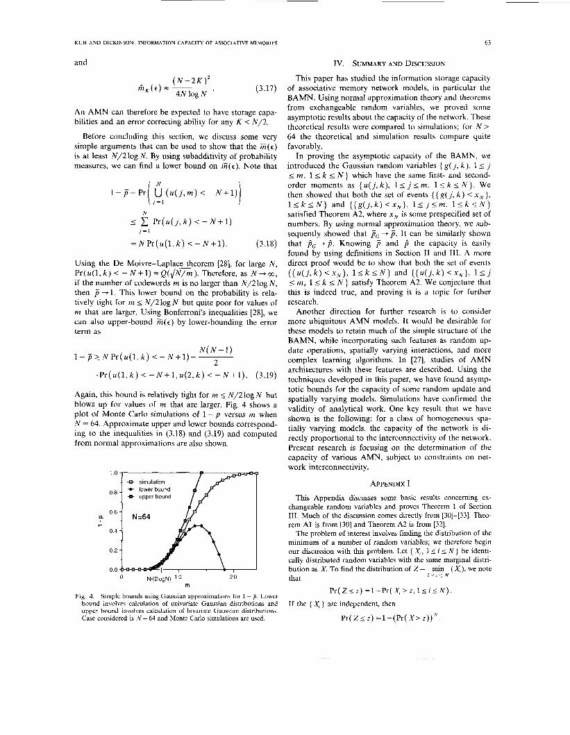
Again, this bound is relatively tight for m 2 N/2log N but blows up for values of m that are larger. Fig. 4 shows a plot of Monte Carlo simulations of 1 - j versus m when N = 64. Approximate upper and lower bounds corresponding to the inequalities in (3.18) and (3.19) and computed from normal approximations are also shown.

Q simulation

0 N/(2logN) 2 0 m

Simple bounds using Gaussian approximations for 1 - p . Lower bound involves calculation of univariate Gaussian distributions and upper bound involves calculation of bivariate Gaussian distributions. Case considered is N = 64 and Monte Carlo simulations are used.

Fig. 4.

63

IV. SUMMARY AND DISCUSSION

This paper has studied the information storage capacity of associative memory network models, in particular the BAMN. Using normal approximation theory and theorems from exchangeable random variables, we proved some asymptotic results about the capacity of the network. These theoretical results were compared to simulations; for N > 64 the theoretical and simulation results compare quite favorably.

In proving the asymptotic capacity of the BAMN, we introduced the Gaussian random variables { g( j , k ) , 1 I j - < m, 1s k N } which have the same first- and second- order moments as {U( j , k), 1 I j m, 1 I k I N }. We then showed that both the set of events { { g ( j , k) < xN}, I s k I N } and {{g< j ,k )<x ,} , 1 1 j < m , l < k < N } satisfied Theorem A2, where x N is some prespecified set of numbers. By using normal approximation theory, we sub- sequently showed that j G -+ j. It can be similarly shown that j G + j . Knowing p and j the capacity is easily found by using definitions in Section I1 and 111. A more direct proof would be to show that both the set of events { { U ( j , k ) < x N } , 1 1 k < N } and { { ~ < j , k ) < x , } , 11j - < m, 1s k I N } satisfy Theorem A2. We conjecture that this is indeed true, and proving it is a topic for further research.

Another direction for further research is to consider more ubiquitous AMN models. It would be desirable for these models to retain much of the simple structure of the BAMN, while incorporating such features as random update operations, spatially varying interactions, and more complex learning algorithms. In [27], studies of AMN architectures with these features are described. Using the techniques developed in this paper, we have found asymptotic bounds for the capacity of some random update and spatially varying models. Simulations have confirmed the validity of analytical work. One key result that we have shown is the following: for a class of homogeneous spatially varying models, the capacity of the network is directly proportional to the interconnectivity of the network. Present research is focusing on the determination of the capacity of various AMN, subject to constraints on network interconnectivity.

APPENDIX I

This Appendix discusses some basic results concerning exchangeable random variables and proves Theorem 1 of Section 111. Much of the discussion comes directly from [30]-[33]. Theo- rem A1 is from [30] and Theorem A2 is from [32].

The problem of interest involves finding the distribution of the minimum of a number of random variables; we therefore begin our discussion with this problem. Let { X,, 1 I i I N } be identically distributed random variables with the same marginal distribution as X . To find the distribution of Z = min ( X , ) , we note that I s r % N

Pr( Z 5 z) =I - Pr( X, > z , 11 i I N ) .

If the { X, } are independent, then

P r (Z<z) = l - (P r (X> z))” .


Let us consider a weaker condition on the { X, }, We say that random variables { X,, 1 I i I N } are exchangeable if their joint

ables. We also define events { C,, 1 I i I N } as exchangeable if, for all choices of indices 1 I i, < . . . < i , I N, we have

(A.1)

Note that ak depends only on k and not on the indices i,. ak will be referred to as the kth De Finetti constant with a, =l. Denot-

where W is a random variable with

distribution is invariant under permutations of the random vari- Pr( W = j) =U,. (A.7)

If we can find the distribution of W, we can find the order statistics of { X,, 1 I i I N } for N finite. This distribution is not easy to determine, but Galambos [32] and Kendall [30] have obtained some results for the limiting case under some mild restrictions.

Pr( c,I,c,2,' ' . ,c,k) = a , , 1 I k I N .

ingtheevent{X,>x}byC, , i f {X, , l I i IN}areexchangeab le random variables, then { C,, 1 I i I N } are exchangeable events. De Finetti [34] proved an important theorem relating exchangeable random variables to conditional distributions.

Theorem A I : Let A ( N ) be the number of C, = { X, > x } that occur for exchangeable random variables X,, 1 I i I N. Then

exists almost surely, and if B (a probability measure on the interval [0,1]) is the distribution function of 5 , then

This result was later extended by several people [35]-[36], giving the following corollary.

Corollary: Given the above conditions there exists a random variable A such that

Pr(C,,,. . .,C1,lA) = th where .$ = A almost surely.

The above results deal with the limiting case as N + co, but we are concerned primarily with finite N . Kendall [30] generalized the above theorems for N finite. As a simple analogy, N = cc can be viewed as picking marbles from a collection of marbles in an urn and replacing the picked marbles, whereas N finite can be viewed as performing the same operation without replacement. If we let 8 ( a k ) = a, - ( Y ~ + ~ , 1 I k I N and 8'(ak) = 8 ( 8 J - ' ( a , ) ) then

N - m

a , ,= 1 ( N i m ) 8 s ( a N - , ) , O s m I N . (A.2)

If we let w/ = ( 7 ) sN-'(a,) for 0 I j I N, then w is a probability distribution since

s = o

F O L , . + ~ ~ O , O i r i N (A.3) and

N

w , = l . (A.4) r = O

Then we have

Theorem A 2 : Let { X,, 1 I i I n} be random variables with corresponding distribution functions { q ( x ) , 1 I i I n } . Let { x , , } be a sequence of real numbers such that

n lim x F ; ( x , , ) = b

n - m

with 0 < b < CO. Setting

where the sum is over all indices 1 I i , < i , < . . . < i, I n. As- sume that for n > no there exists a,(n), n < j < M,, such that sequence a/ ( n ) , 1 I j < M,, can be associated with a set of M,, exchangeable events. If M,, = cc for n > no or if both M,, /n + 00

and n + 00 with

Iim n2a2( n) = b2, n - r m

then for any j ,

where xJ* is the jth-order statistic. The above theorem has the following intuitive interpretation.

We construct M, exchangeable events from some set of n random variables with M,, >> n. If the events are nearly painvise independent, then I of these events are nearly jointly independent for 2 I I I n . A proof of this theorem presented in [30] is based on finding the characteristic function of K,, =E.:'=lI( X, < x, , ) and approximating this with the characteristic function of a Poisson random variable with parameter b. The approximation uses Chebyshev's inequality and depends only on the quantities I n q ( n ) - bl and ln2az(n)- b21 and not on b.

In the problem of interest in Section 111, for some N and m we want to find Pr(min ( g ( i , j ) , 1 I i I N ) < - N + 1) and Pr(min( g(i, j ) , 1 I i I N , 1 I j I m ) < - N + 1) where the { g ( i , j )} are Gaussian exchangeable random variables. We first normalize these random variables, obtaining random variables { G,,( i , j )} with the following second moments:

I-

(A'5) E [ G , , ( i , j)G,,(k,l)] = / T' m - 1 '

i i t k , j = l

i = k , j + l

1 I ( n -I)( m - 1) ' otherwise.

I w\, \ k l Pr(C,,,C,2,. . . , C , p J ) = __ (A'6) We want to find the values of m where Theorem A2 can be

applied to evaluate the two problems of Section 111. To use

Kun AND DICKINSON: INFORMATION CAPACITY OF ASSOCIATIVE MEMORIES 65

Theorem A2 to evaluate

Pr(min( g( i, j ) , 1 I i I N) < - N + 1) = Pr(min( G N ( i , j ) , 11 i I N ) < x , ) ,

the following two conditions must hold for all n 2 N:

1) lim,,,, n2a2(n) = b2; 2) there exists M,, such that M,,/n + 03 as n + cc with the

set { G,,(i, j ) , 1 I i I n } augmented to 1 I i I M,, elements so that all G,,(i, j ) are still exchangeable.

Here b is determined by fixing N and setting b = NQ( - x , ) where x , = -,/( N-l) / (rn-1) . x,, are chosen such that rial( n ) = b and therefore x , = - Q-'(b/n).

Condition 2) is easy to show because we can always add any number of Gaussian random variables to the set {G,,(i, j ) , 1 I i I n} with all the random variables having the desired first- and second-order moments. By the definition of exchangeability this new augmented set has members that are still exchangeable.

For 1) we want to find the values of m where

lim n2a2( n) - b2 = 0. ('4.8) n + m

Let f , ( x , y ) be the bivariate Gaussian density function with marginals having mean 0 and variance 1, and correlation p. Also let F,(Z) be the distribution function of Z = max(X,Y) where X and Y are the marginals of the bivariate Gaussian distribution with correlation p . Let y = 1/( n - 1). Then (A.8) is equivalent to

lim n 2 F ( x , ) = b2. (A.9) n + m

Note that

have that

(A.14) 1

/( - x , , ) = -n- ' l2 J2n From (A.14) as n + cc

Equation (A.9) is satisfied when a > 1. If we set m = N / c log N, then x,, = - ,/*. If c > 1 then for all n 2 N , it is easily shown that x,, = - ,/* where c,, > 1. Therefore, (A.15) is satisfied for all n 2 N provided that m < N/log N . Recall that b and therefore N are independent of the covergence in distribution of K , to a Poisson random variable with parameter b. Using these facts, we can therefore state that for rn < N/log N the number of events { G, ( i , j ) < x N }, 1 I i I N occurring converges in distribution (as N + CO) to a Poisson distribution with parameter NQ( - x , ) .

To use Theorem A2 to evaluate

Pr(min( g( i , j ) , 11 i I N, 11 j~ r n ) < - N +1)

= Pr(min( G, ( i , j ) , 1 I i I N, 1 I j I m ) < x , ) ,

we again need two conditions analogous to those just obtained for all n 2 N . For Gaussian exchangeable random variables the second condition is trivial to show, just as in the previous case. For the first condition we require that

lim n2rn2( a2( n)) = b'. (A.16)

For this case x,, = - Q-'(b/nrn) and b = NmQ( - x, ) . We again use the Hermite polynomial expansion of the bivariate density to show that

n + m

We first look at the inner integrand. f , ( x , y ) can be expanded as a product of the two marginal density functions (f( x ) and f( y ) ) , and a series expansion involving Hermite polynomials HI ( x ) [37]

where

Equation (A.lO) can then be written as

(A.12)

(A.13)

Note that Q(- x,!) = b / n and, by setting x,, = -,/-, we

where yl = 1/( n - l), y2 = 1/( rn - l ) , and y3 = 1/( n - 1)( m - 1). From (A.14) and (A.16) as n -+ 03

+ O ( n - " ( a l ~ g n ) ~ ) . (A.18) a log n 1

Equation (A.9) is satisfied when a 2 2. Using the same arguments as in the first case, we can state that for rn I N/2log N the number of events { G N ( i , j ) < x , } , 1 I i I N , 15 j I m occurring converges in distribution (as N + 03) to a Poisson distribution with parameter NrnQ(- x, ) . We have thus proved the following theorem which is identical to the theorem in Section 111.

Theorem A3: 1) If

and Y, is a Poisson random variable with parameter A, =

NQ(JN/m), then X, -+ Y, in distribution.


2) If

and YN is a Poisson random variable with parameter A, =

N m Q ( m ) , then X,, + Y,, in distribution.

APPENDIX I1

Given the random variables {U( j , k ) , 1 I j I N } defined in Section 111, we want to find the following probability:

p = P r n u ( j , k ) > - N + l , l i k i m (B.1)

where { U( j , k ) } are binomial random variables with E( U( j , k ) ) =Oand

i N ;=1 i ( N -1)( m -l), j = I

j # l . E (u ( j , k )u ( l , k ) ) =

From (3.2) we note that each u ( j , k ) is the sum of m - 1 independent identically distributed (i.i.d.) random variables. Let us normalize these random variables, defining

For large m we know that U( j ) converges to a standard Gaus- sian random variable (mean 0 and variance 1) by the central limit theorem. This theorem is also applicable to multivariate distributions; the N-variate joint distribution of { U ( j ) , 1 I j I N } thus converges to the multivariate Gaussian distribution N(0, R ) where

R ( i . = 1 i Z j

as m grows large; see [29, 38, 391.

variables, the results of Appendix I show that Under the assumption that the { U ( j )} are Gaussian random

(B.2) . e-(l/2)XrR-‘-x dx, dx, . . . dx,

where b=, / (N- l ) / (m- l ) and xT=(xl;.. ,xN). Since the Gaussian assumption is only true asymptotically, we are led to the question of whether or not j - j G . In this Appendix we show that p + pc for large m by comparing the normal approximation of {U(j), 15 j I N} to { U ( j ) , 11 j < N}. We first state some necessary results from normal approximation theory.

A. Error Terms in the Normal Approximation to i.i.d, Random Vectors

Let us first look at the problem of approximating the distribution of sums of i.i.d. random variables by the normal distribution in R’. We want to find how “close” the normal distribution is to the distribution of a normalized finite sum of i.i.d. random variables. Let {U,, 1 I i I m } be N i.i.d. random variables with Eu, = 0, Eu; =1, and let

Then the difference between F,,(x) , the distribution of U,,, and the standard normal distribution @(x) is given by

m

F , , ( x ) - @ ( x ) % + ( X I Q , ( X ) ~ - ” ~ 03.3) I =1

where +(x) is the probability density function of the standard normal distribution and Q, (x) are polynomials derived from the standard Hermite polynomials [37]:

with

Letting f , , ( x ) be the probability density function of F,,(x) , we have

We would like to find the order of magnitude of error terms in (B.3). In particular, we are interested in the size of F,,( x) - Q (x) - [+(x)Ql(x)/&I.

For lattice (i.e., discrete) distributions where all sample values can be expressed in the form a + ih where a and h are constants and i is an integer, the following result holds [40], [41]:

(B.4)

where S,( .) is a correction term arising from the discontinuities of the distribution function and h is the size of the lattice. The correction term is the periodic function

S,(x) =xmod(l)-0.5. (B.5)

For distributions in R N an approximation analogous to (B.4) is slightly more complicated. Now let {U, } be random vectors with Eu, = 0 and EuTu, = R . Before stating a theorem from [38] we present some definitions. Let f , ( t ) be the characteristic function of the distribution F, (x). The characteristic function can be expressed in the following way:

where Y is a nonnegative integer vector, v ! = r I ~ , v , ! , (it)” =

rIy=l(it)”f, and I Y I =Cr=lv,. The coefficients x, are called the semi-invariants of F,,. For a Gaussian random vector all semi- invariants for I Y I > 2 are 0. Also define

a p D”f( x) = ax: ax;2 . . . ax? ( x ) (B.7)

and

The following theorem from [38] can now be stated.

KUH AND DICKINSON: INFORMATION CAPACITY OF ASSOCIATIVE MEMORIES 67

<m-’/Z h / ~ l ( B ~ / h / ) ~ , ( ~ ~ , R ( P ) ) j = l I N -

Theorem B1: Let F , , ( x ) be defined as above. Then Using the fact that the random variables we are looking at are exchangeable and using (B.lO)-(B.13), we have that I F,z( x , - ‘ 0 , R ( I

networks: an A/D converter, signal decision circuit, and a linear programming circuit,” IEEE Trans. Circuits S-yst., vol. CAS-33, pp. 533-541,1986.

x € R N

Equation (B.8) is similar to (B.4) in that the first term on the

O( m- 1/2) error that occurs for all distributions.

(1 +2P) P

(1 + ( N - l ) P ) ( l + P ) + (N-Z)+(P, P 7 P ) right side of the equation is an error term due to the lattice

distribution, and the second term describes the standard

+ 7 + ( P A P ) ) 1 B. Using Normal Approximation Theory to Show that j + j c

1/-. We define the vth moment as

+ o( m-l/’). (B.15) We now show that p + p G . For U(j) we have h=h,=

Substituting values of m and p and simplifying, we have

alogN N-“/’ r- pv = /J . . . /xvfm ( x ) dx , dx , . . . d x , 03.9)

where x” = flElx:z and f m ( x ) is the N-variate joint density function of { U ( j ) , 1 I j I N } . For the case where x, = 0 for [ V I = 1 it is easily shown that pv = x, when I Y I = 3. The semi- invariants we need to use in (B.8) are taken from the following third moment values:

E U ( i ) U( j) U( k) = I‘ - 7

( a log N)3/2 N(’/2)-(3“/2)5a log N + N(1/2)-0 + . (B.16)

27T 6 ( 2 a ) 3 / 2

i = j = k When 1/2 < a << N/log N, lj - jGl+ 0 as N -+ CO. Asymptoti- cally, we are only interested in the area around a = 2. For a < 2, jG .+ 1 and for a 2 2, j G + 0. Therefore, we can state that

2(N-2) i = j # k

2 j = e - N Q ( P ) i # j , i # k , j # k .

(B.lO) as N grows large.

(B.17)

We also observe that

(B.ll)

68 IEEE TRANSACTIONS ON lNFORMATION THEORY, VOL. 35, NO. 1, JANUARY 1989

[8] H. P. Graf et al., “VLSI implementation of a neural network memory with several hundred neurons,” in A I P Conf. Proc. 151, Neurul Networks for Computing, Snowbird, UT, 1986, pp. 182-188. D. Psaltis and Y. S. Abu-Mostafa, “Computation power of paral- lelism in optical computers,” Dep. Elec. Eng., Calif. Inst. Technol., Pasadena, preprint, 1985. D. Psaltis, J. Hong, and S. S. Venkatesh, “Shift invariance in optical associative memories,” Dep. Elec. Eng., Calif. Inst. Technol., Pasadena, preprint, 1986. Y. S. Abu-Mostafa and J. M. St. Jacques, “Information capacity of the Hopfield model,” IEEE Trans. Inform. Theory, vol. IT-31, pp. 461-464, 1985. R. J . McEliece, E. C. Posner, E. R. Rodemich, and S. S. Venkatesh, “The capacity of the Hopfield associative memory,” IEEE Truns. Inform. Theory, vol. IT-33, pp. 461-482, 1987.

[13] D. 0. Hebb, The Orgunizution of Behavior. New York: Wiley, 1949.

1141 T. Kohonen, Self-Orgunizntion and Associative Memory. Berlin, Germany: Springer-Verlag, 1984.

[15] -, Content Addressable Memories. New York: Springer-Verlag, 1980.

[16] W. A. Little, “The existence of persistent states in the brain,” Math. Biosci., vol. 19, pp. 101-120, 1974.

1171 W. A. Little and G. L. Shaw, “Analytic study of the memory storage capacity of a neural network,” Muth. Eiosci., vol. 39, pp. 281-290, 1978.

[18] S. Amari, “Neural theory of association and concept formation,” Biol. Cyhern., vol. 26, pp. 175-185, 1977.

[19] ~, “A method of statistical neurodynamics,” Kybernetik, vol.

[20] K. Nakano, “Associatron: A model of associative memory,” IEEE Trans. S-yst. Man Cybern., vol. SMC-2, pp. 380-388, 1972.

1211 G. E. Hinton and J. A. Anderson, Parallel Models of Associative Memory. Hillsdale, NJ: Erlbaum, 1981.

[22] D. J. Willshaw, 0. P. Buneman, and H. C. Longuet-Higgins, “ Non-holographic associative memory,’’ Nature, vol. 222, pp. 960-962, 1969. R. Hecht-Nielson, “Artificial neural system technology,” TRW preprint, 1986. S. S. Venkatesh and D. Psaltis, “Information storage and retrieval in two associative nets,” Dep. Elec. Eng., Calif. Inst. Technol., Pasadena, preprint, 1985.

[9]

[lo]

1111

1121

12, pp. 201-215, 1974.

[23]

1241

S. S. Venkatesh, “Epsilon capacity of neural networks,” Dep. Elec. Eng., California Institute of Technology, Pasadena, preprint, 1986. N. Rochester, J. H. Holland, L. H. Haibt, and W. L. Duda, “Tests on a cell assembly of the action of the brain, using a large digital computer,” IRE Truns. Inform. Theoty, vol. IT-2, no. 3, pp. 80-93, 1956. A. Kuh, “Stochastic models for interacting systems,” Ph.D. disser- tation, Princeton Univ., Princeton, NJ, 1986. W. Feller, A n Introduction to Probability Theory and its Applicu- tions, vol. 1. -, A n Introduction to Probability Theory and its Applicutions, vol. 2. D. G. Kendall, “On finite and infinite sequences of exchangeable events,” Studia Sci. Math. Hungar., vol. 2, pp. 319-327, 1967. C. J. Ridler Rowe, “On two problems of exchangeable events,” Studiu Sci. Math. Hungnr., vol. 2, pp. 415-418, 1967. J. Galambos, “A general Poisson limit theorem of probability theory,” Duke Muth. J., vol. 40, pp. 581-586,1973. Y . S. Chow and H. Teicher, Prohahilip Theory: Independence, Interchangeability, Martingules. New York: Springer-Verlag, 1978. B. De Finetti, “Funzione caratteristica di un fenomeno aleatorio.” Atti. Accud. Nuz. Lincei. Rend. SI. Sci. Fis. Mat. Nut., (6) 4, pp. 86-133, 1930. E. Hewitt and L. J. Savage, “Symmetric measures on Cartesian products,” Trans. Amer. Math. Soc., vol. 80, pp. 470-501, 1955. A. Renyi and P. Revesz, “A study of sequences of equivalent events as special stable sequences,” Publ. Math. Dehrecen., vol. 10, pp.

J. B. Thomas, A n Introduction to Statistical Communication Theoty. New York: Wiley, 1968. R. N. Bhattacharya and R. R. Rao, Normal Approximution and Asymptotic Expansions. H. Cramer, Random Variables and Probability Distributions. Cam- bridge Univ. Press, 1937. C. G. Esseen, “Fourier analysis of distribution functions. A mathe- matical study of the Laplace-Gaussian law,” Acta Math., vol. 77, pp. 1-125, 1945. A. C. Berry, “The accuracy of the Gaussian approximation to the sum of independent variates,” Trans. Amer. Muth. Soc., vol. 48, pp. 122-136, 1941. H. 0. Lancaster, “The structure of bivariate distributions,” Ann. Muth. Statist., vol. 29, pp. 719-736, 1958.

New York: Wiley, 1950.


319-325, 1963.


Documents

Information capacity of associative memories