Information and Computation 243 (2015) 263–280

Contents lists available at ScienceDirect

Information and Computation

www.elsevier.com/locate/yinco

Distributed coloring algorithms for triangle-free graphs

Seth Pettie, Hsin-Hao Su ∗

University of Michigan, Ann Arbor, MI 48105, United States

a r t i c l e i n f o a b s t r a c t

Article history:Received 8 September 2013Available online 12 December 2014

Vertex coloring is a central concept in graph theory and an important symmetry-breaking primitive in distributed computing. Whereas degree-Δ graphs may require palettes of Δ +1colors in the worst case, it is well known that the chromatic number of many natural graph classes can be much smaller. In this paper we give new distributed algorithms to find (Δ/k)-coloring in graphs of girth 4 (triangle-free graphs), girth 5, and trees. The parameter k can be at most ( 1

4 −o(1)) lnΔ in triangle-free graphs and at most (1 −o(1)) lnΔ in girth-5 graphs and trees, where o(1) is a function of Δ. Specifically, for Δ sufficiently large we can find such a coloring in O (k + log∗ n) time. Moreover, for any Δ we can compute such colorings in roughly logarithmic time for triangle-free and girth-5 graphs, and in O (log Δ +logΔ log n) time on trees. As a byproduct, our algorithm shows that the chromatic number of triangle-free graphs is at most (4 + o(1)) Δ

ln Δ, which improves on Jamall’s recent bound

of (67 + o(1)) Δln Δ

. Finally, we show that (Δ + 1)-coloring for triangle-free graphs can be obtained in sublogarithmic time for any Δ.

© 2014 Published by Elsevier Inc.

1. Introduction

A proper t-coloring of a graph G = (V , E) is an assignment from V to 1, . . . , t (colors) such that no edge is monochro-matic, or equivalently, each color class is an independent set. The chromatic number χ(G) is the minimum number of colors needed to properly color G . Let Δ be the maximum degree of the graph. It is easy to see that sometimes Δ + 1 colors are necessary, e.g., on an odd cycle or a (Δ + 1)-clique. Brooks’ celebrated theorem [9] states that these are the only such examples and that every other graph can be Δ-colored. Vizing [38] asked whether Brooks’ Theorem can be improved for triangle-free graphs. In the 1970s Borodin and Kostochka [8], Catlin [10], and Lawrence [27] independently proved that χ(G) ≤ 3

4 (Δ + 2) for triangle-free G , and Kostochka (see [20]) improved this bound to χ(G) ≤ 23 (Δ + 2).

Existential bounds Better asymptotic bounds were achieved in the 1990s by using an iterated approach, often called the “Rödl Nibble”. The idea is to color a very small fraction of the graph in a sequence of rounds, where after each round some property is guaranteed to hold with some small non-zero probability. Kim [22] proved that in any girth-5 graph G , χ(G) ≤(1 + o(1)) Δ

ln Δ. This bound is optimal to within a factor-2 under any lower bound on girth. (Constructions of Kostochka

and Mazurova [24] and Bollobás [7] show that there is a graph G of arbitrarily large girth and χ(G) > Δ2 ln Δ

.) Building

This work is supported by NSF CAREER grant CCF-0746673, NSF grants CCF-1217338 and CNS-1318294, and a grant from the US–Israel Binational Science Foundation, 2008390.

* Corresponding author.E-mail address: hsinhao@umich.edu (H.-H. Su).

http://dx.doi.org/10.1016/j.ic.2014.12.0180890-5401/© 2014 Published by Elsevier Inc.

264 S. Pettie, H.-H. Su / Information and Computation 243 (2015) 263–280

on [22], Johansson (see [30]) proved that χ(G) = O ( Δln Δ

) for any triangle-free (girth-4) graph G .1 In relatively recent work Jamall [17] proved that the chromatic number of triangle-free graphs is at most (67 + o(1)) Δ

ln Δ.

Algorithms We assume the LOCAL model [33] of distributed computation. In this model, vertices host processors which operate in synchronized rounds; vertices can communicate one arbitrarily large message across each edge in each round; local computation is free; time is measured by the number of rounds. Grable and Panconesi [15] gave a distributed algorithm that Δ/k-colors a girth-5 graph in O (log n) time, where Δ > log1+ε n and k ≤ δ ln Δ for any ε > 0 and some δ < 1 depending on ε .2 Jamall [18] showed a sequential algorithm for O (Δ/ ln Δ)-coloring a triangle-free graph in O (nΔ2 ln Δ) time, for any ε > 0 and Δ > log1+ε n.

Note that there are two gaps between the existential [22,30,17] and algorithmic results [15,18]. The algorithmic results use a constant factor more colors than necessary (compared to the existential bounds) and they only work when Δ ≥log1+Ω(1) n is sufficiently large, whereas the existential bounds hold for all Δ.

New results We give new distributed algorithms for (Δ/k)-coloring triangle-free graphs that simultaneously improve on both the existential and algorithmic results of [15,30,17,18]. Our algorithms run in log1+o(1) n time for all Δ and in O (k +log∗ n) time for Δ sufficiently large. Moreover, we prove that the chromatic number of triangle-free graphs is (4 + o(1)) Δ

ln Δ.

Theorem 1. Fix a constant ε > 0. Let Δ be the maximum degree of a triangle-free graph G, assumed to be at least some Δε depending on ε . Let k ≥ 1 be a parameter such that k ≤ 1

4 (1 − 2ε) ln Δ. Then G can be (Δ/k)-colored, in time O (k + log∗ Δ) if Δ1− 4kln Δ

−ε =Ω(ln n), and, for any Δ, in time on the order of

(k + log∗ Δ

) · lnn

Δ1− 4kln Δ

−ε· exp

(O (

√ln ln n)

) = (ln n)1+O (1/√

ln ln n) = ln1+o(1) n.

The first time bound comes from an O (k + log∗ Δ)-round procedure, each round of which succeeds with probability 1 − 1/ poly(n). However, as Δ decreases the probability of failure tends to 1. To enforce that each step succeeds with high probability we use a version of the Local Lemma algorithm of Moser and Tardos [31] optimized for the parameters of our problem.

Theorem 1 has a complex tradeoff between the minimum threshold Δε , the number of colors, and the threshold for Δbeyond which the running time becomes O (log∗ n). The following corollaries highlight some interesting parameterizations of Theorem 1.

Collorary 1. The chromatic number of triangle-free graphs with maximum degree Δ is at most (4 + o(1))Δ/ ln Δ.

Proof. Fix an ε′ > 0 and choose k = ln Δ/(4 + ε′) and ε = ε′/(2(4 + ε′)). Theorem 1 states that for Δ at least some Δε′ , the chromatic number is at most (4 + ε′)Δ/ ln Δ. Now let ε′ = o(1) be a function of Δ tending slowly to zero. (The running time of the algorithm that finds such a coloring is never more than (ln n)1+O (1/

√ln ln n) .)

Collorary 2. Fix any δ > 0. A (4 + δ)Δ/ ln Δ-coloring of an n-vertex triangle-free graph can be computed in O (log∗ n) time, provided Δ > (ln n)(4+δ)δ−1+o(1) and n is sufficiently large.

Proof. Set k = ln Δ/(4 + δ) and let ε = o(1) tend slowly to zero as a function of n. If we have

Δ1−4k/ ln Δ−ε = Δ1−4/(4+δ)−ε = Δδ(4+δ)−1−ε = Ω(lnn),

or equivalently, Δ > (ln n)δ−1(4+δ)+o(1) , then a (4 + δ)Δ/ ln Δ-coloring can be computed in O (log∗ n) time. (For n sufficiently

large and ε tending slowly enough to zero, the lower bound on Δ also implies Δ > Δε .) Theorem 1 also shows that some colorings can be computed in sublogarithmic time, even when Δ is too small to achieve

an O (log∗ n) running time.

Collorary 3. Fix a δ > 0 and let k = o(ln Δ). If Δ > (ln n)δ , a (Δ/k)-coloring can be computed in (lnn)1−δ+o(1) time.

1 We are not aware of any extant copy of Johansson’s manuscript. It is often cited as a DIMACS Technical Report, though no such report exists. Molloy and Reed [30] reproduced a variant of Johansson’s proof showing that χ(G) ≤ 160 Δ

ln Δfor triangle-free G .

2 They claimed that their algorithm could also be extended to triangle-free graphs. Jamall [18] pointed out a flaw in their argument.

S. Pettie, H.-H. Su / Information and Computation 243 (2015) 263–280 265

Proof. Let ε = o(1) tend slowly to zero as a function of n. The running time of Theorem 1 is on the order of

(k + log∗ Δ

) · ln n

Δ1− 4kln Δ

−ε· exp

(O (

√ln ln n)

) = O

(ln n

Δ1−o(1)−ε−ln k/ ln Δ· exp

(O (

√log log n)

))

= O((ln n)1−δ+o(1)+O (1/

√ln ln n)

)= (ln n)1−δ+o(1).

Our result also extends to girth-5 graphs with Δ1− 4kln Δ

−ε replaced with Δ1− kln Δ

−ε . This change allows us to (1 +o(1))Δ/ ln Δ-color such graphs. Our algorithm can clearly be applied to trees (girth ∞). Elkin [13] noted that with Bol-lobás’s construction [7], Linial’s lower bound [28] on coloring trees can be strengthened to show that it is impossible to o(Δ/ ln Δ)-color a tree in o(logΔ n) time. We prove that it is possible to (1 + o(1))Δ/ ln Δ-color a tree in O (log Δ +logΔ log n) time. Also, we show that a (Δ + 1)-coloring in triangle-free graphs can be computed in exp(O (

√log log n)) time,

independent of Δ, which improves on the O (log Δ + exp(O (√

log log n))) time algorithm for arbitrary graphs [5].A graph is called k-list-colorable if it can be properly colored when each vertex is assigned an arbitrary palette of k

colors. Without modifying the analysis, our results extend to list-coloring triangle-free graphs and girth-5 graphs. E.g., we can (4 + o(1)) Δ

ln Δ-list-color triangle-free graphs. However, our result for trees cannot be extended for list-coloring. The

algorithm reserves a set of colors for a final coloring phase and these colors must be in the palette of every vertex. In list-coloring, it is not possible to reserve such a set of colors.

Technical overview Intuitively, consider a vertex u with its Δ neighbors. Suppose that each of its neighbor is colored with a color from one of the cΔ/ ln Δ colors uniformly at random, where c is a constant. Then the expected number of colors not chosen by u’s neighbor is at least Δ · (1 − 1/(cΔ/ ln Δ))Δ ∼ Δ1−1/c . When c > 1, it is likely there will be colors not colored by u’s neighbor and so u can be colored by using one of them. The iterated approaches of [22,15,30,17] manage to achieve the situation where each vertex in the neighborhood is colored uniformly at random, round by round.

In the iterated approaches, each vertex u maintains a palette, which consists of the colors that have not been selected by its neighbors. To obtain a t-coloring, each palette consists of colors 1, . . . , t initially. In each round, each uncolored u tries to assign itself a color (or colors) from its palette, using randomization to resolve the conflicts between itself and the neighbors. The c-degree of u is defined to be the number of its neighbors whose palettes contain c. In Kim’s algorithm [22] for girth-5 graphs, the properties maintained for each round are that the c-degrees are upper bounded and the palette sizes are lower bounded. In girth-5 graphs the neighborhoods of the neighbors of u only intersect at u and therefore have a negligible influence on each other, that is, whether c remains in one neighbor’s palette has little influence on a differ-ent neighbor of u. Due to this independence one can bound the c-degree after an iteration using standard concentration inequalities. In triangle-free graphs, however, there is no guarantee of independence. If two neighbors of u have identical neighborhoods, then after one iteration they will either both keep or both lose c from their palettes. In other words, the c-degree of u is a random variable that may not have any significant concentration around its mean. Rather than bound c-degrees, Johansson [30] bounded the entropy of the remaining palettes so that each color is picked nearly uniformly in each round. Jamall [17] claimed that although each c-degree does not concentrate, the average c-degree (over each c in the palette) does concentrate. Moreover, it suffices to consider only those colors within a constant factor of the average in subsequent iterations.

Our (Δ/k)-coloring algorithm performs the same coloring procedure in each round, though the behavior of the algorithm has two qualitatively distinct phases. In the first O (k) rounds the c-degrees, palette sizes, and probability of remaining uncolored vertices are very well behaved. Once the available palette is close to the number of uncolored neighbors, the probability a vertex remains uncolored begins to decrease drastically in each successive round, and after O (log∗ n) rounds all vertices are colored, w.h.p.

Our analysis is similar to that of Jamall [17] in that we focus on bounding the average of the c-degrees. However, our proof needs to take a different approach, for two reasons. First, to obtain an efficient distributed algorithm we need to obtain a tighter bound on the probability of failure in the last O (log∗ n) rounds, where the c-degrees shrink faster than a constant factor per round. Second, there is a small flaw in Jamall’s application of Azuma’s inequality in Lemma 12 in [17], the corresponding Lemma 17 in [18], and the corresponding lemmas in [19]. It is probably possible to correct the flaw, though we manage to circumvent this difficulty altogether. See Appendix A for a discussion of this issue.

The second phase presents different challenges. The natural way to bound c-degrees using Chernoff-type inequalities gives error probabilities that are exponential in the c-degree, which is fine if it is Ω(log n) but becomes too large as the c-degrees are reduced in each coloring round. At a certain threshold we switch to a different analysis (along the lines of Schneider and Wattenhofer [37]) that allows us to bound c-degrees with high probability in the palette size, which, again, is fine if it is Ω(log n).

In both phases, if we cannot obtain small error probabilities (via concentration inequalities and a union bound) we revert to a distributed implementation of the Lovász Local Lemma algorithm [31,11]. We show that for certain parameters the symmetric LLL can be made to run in sublogarithmic time. For the extensions to trees and the (Δ + 1)-coloring algorithm for triangle-free graphs, when we cannot obtain small error probabilities, we will ignore those bad vertices where error

266 S. Pettie, H.-H. Su / Information and Computation 243 (2015) 263–280

occured. Using the ideas from [5,6,36], we can show the size of each component induced by the bad vertices is at most polylog(n). Each component can then be colored separately in parallel by the deterministic algorithms [4,32], which now runs faster as the size of each subproblem is smaller.

Organization Section 2 introduces some basic probabilistic tools. Section 3 presents the general framework for the analysis. Section 4 describes the algorithms and discusses what parameters to plug into the framework. Section 5 describes extensions of the algorithm to graphs of girth 5, trees, and the (Δ + 1)-coloring problem for triangle-free graphs.

2. Tools

See Dubhashi and Panconesi [12] for proofs of Lemma 1, Lemma 2, and related concentration bounds.

Lemma 1 (Hoeffding’s inequaliy). Let X1, . . . , Xn be independent random variables such that ai ≤ Xi ≤ bi for 1 ≤ i ≤ n. Let X = ∑i Xi ,

then for any t > 0,

Pr(

X > E[X] + t) ≤ e

− 2t2∑i (bi−ai )

2

Lemma 2 (Chernoff bound). Let X1, . . . , Xn be independent 0/1 random variables such that Pr(Xi = 1) = p. Let X = ∑ni=1 Xi . Then,

for δ > 0:

Pr(

X > (1 + δ)E[X]) ≤[

eδ

(1 + δ)(1+δ)

]E[X]

Pr(

X < (1 − δ)E[X]) ≤[

e−δ

(1 − δ)(1−δ)

]E[X]

The two bounds above imply that for 0 < δ < 1, we have:

Pr(

X > (1 + δ)E[X]) ≤ e−δ2 E[X]/3

Pr(

X < (1 − δ)E[X]) ≤ e−δ2 E[X]/2.

Collorary 4. Let X1, . . . , Xn be independent 0/1 random variables such that Pr(Xi = 1) = pi . Let X = ∑ni=1 Xi . If M ≥ E[X] and

0 < δ < 1, then

Pr(

X > E[X] + δM) ≤ e−δ2 M/3.

Proof. Without loss of generality, assume M = t E[X] for some t ≥ 1, we have

Pr(

X > E[X] + δM) ≤

[etδ

(1 + tδ)(1+tδ)

]E[X]by Lemma 2

=[

eδ

(1 + tδ)(1+tδ)/t

]M

≤[

eδ

(1 + δ)(1+δ)

]M

(∗)

≤ e−δ2 M/3 eδ

(1 + δ)(1+δ)≤ e−δ2/3 for 0 < δ < 1

(∗) follows if (1 + tδ)(1+tδ)/t ≥ (1 + δ)(1+δ) , or equivalently, ((1 + tδ)/t) ln(1 + tδ) ≥ (1 + δ) ln(1 + δ). Letting f (t) =((1 + tδ)/t) ln(1 + tδ) − (1 + δ) ln(1 + δ), we have f ′(t) = ln( 1+δt

1+δ) and f ′′(t) = δ

1+δt . Thus, f ′(t) is zero iff t = 1, f (1) = 0, and f ′′(1) = δ

1+δ> 0 imply f (t) ≥ 0 for all t ≥ 1.

The following lemma shows that when conditioning on a likely event B , the probability of an event A can only be affected by Pr(B).

Lemma 3. For any events A and B, it holds that | Pr(A) − Pr(A|B)| ≤ Pr(B).

Proof. Pr(A) = Pr(B) Pr(A|B) +Pr(B) Pr(A|B) = Pr(A|B) +Pr(B)(Pr(A|B) −Pr(A|B)). Therefore, | Pr(A) −Pr(A|B)| ≤ Pr(B).

S. Pettie, H.-H. Su / Information and Computation 243 (2015) 263–280 267

Lemma 4. e−x ≤ 1 − x/2 for 0 ≤ x ≤ 1.59.

Proof. Let f (x) = e−x − 1 + x/2. f (0) = 0 and f (1.59) ≤ 0. f ′(x) = 1/2 − e−x , f ′(x) is zero only when x = ln 2 ≤ 1.59. Since f (ln 2) ≤ 0, f (x) ≤ 0 for 0 ≤ x ≤ 1.59. 3. The framework

Every vertex maintains a palette that consists of all colors not previously chosen by its neighbors. The coloring is per-formed in rounds, where each vertex chooses zero or more colors in each round. Let Gi be the graph induced by the uncolored vertices after round i, so G = G0. Let Ni(u) be u’s neighbors in Gi and let Pi(u) be its palette after round i. The c-neighbors Ni,c(u) consist of those v ∈ Ni(u) with c ∈ Pi(v). Call |Ni(u)| the degree of u and |Ni,c(u)| the c-degree of u after round i. This notation is extended to sets of vertices in a natural way, e.g., Ni(Ni(u)) is the set of neighbors of neighbors of u in Gi .

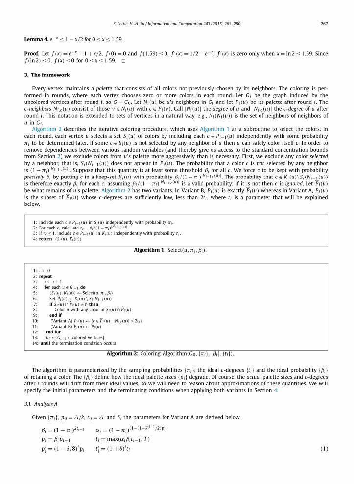
Algorithm 2 describes the iterative coloring procedure, which uses Algorithm 1 as a subroutine to select the colors. In each round, each vertex u selects a set Si(u) of colors by including each c ∈ Pi−1(u) independently with some probability πi to be determined later. If some c ∈ Si(u) is not selected by any neighbor of u then u can safely color itself c. In order to remove dependencies between various random variables (and thereby give us access to the standard concentration bounds from Section 2) we exclude colors from u’s palette more aggressively than is necessary. First, we exclude any color selectedby a neighbor, that is, Si(Ni−1(u)) does not appear in Pi(u). The probability that a color c is not selected by any neighbor is (1 − πi)

|Ni−1,c(u)| . Suppose that this quantity is at least some threshold βi for all c. We force c to be kept with probability precisely βi by putting c in a keep-set Ki(u) with probability βi/(1 −πi)

|Ni−1,c(u)| . The probability that c ∈ Ki(u)\Si(Ni−1(u))

is therefore exactly βi for each c, assuming βi/(1 − πi)|Ni−1,c(u)| is a valid probability; if it is not then c is ignored. Let P i(u)

be what remains of u’s palette. Algorithm 2 has two variants. In Variant B, Pi(u) is exactly P i(u) whereas in Variant A, Pi(u)

is the subset of P i(u) whose c-degrees are sufficiently low, less than 2ti , where ti is a parameter that will be explained below.

1: Include each c ∈ Pi−1(u) in Si(u) independently with probability πi .2: For each c, calculate rc = βi/(1 − πi)

|Ni−1,c (u)| .3: If rc ≤ 1, include c ∈ Pi−1(u) in Ki(u) independently with probability rc .4: return (Si(u), Ki(u)).

Algorithm 1: Select(u,πi, βi).

1: i ← 02: repeat3: i ← i + 14: for each u ∈ Gi−1 do5: (Si(u), Ki(u)) ← Select(u, πi , βi)

6: Set Pi(u) ← Ki(u) \ Si(Ni−1(u))

7: if Si(u) ∩ P i(u) = ∅ then8: Color u with any color in Si(u) ∩ P i(u)

9: end if10: (Variant A) Pi(u) ← c ∈ P i(u) | |Ni,c(u)| ≤ 2ti11: (Variant B) Pi(u) ← P i(u)

12: end for13: Gi ← Gi−1 \ colored vertices14: until the termination condition occurs

Algorithm 2: Coloring-Algorithm(G0, πi, βi, ti).

The algorithm is parameterized by the sampling probabilities πi, the ideal c-degrees ti and the ideal probability βiof retaining a color. The βi define how the ideal palette sizes pi degrade. Of course, the actual palette sizes and c-degrees after i rounds will drift from their ideal values, so we will need to reason about approximations of these quantities. We will specify the initial parameters and the terminating conditions when applying both variants in Section 4.

3.1. Analysis A

Given πi, p0 = Δ/k, t0 = Δ, and δ, the parameters for Variant A are derived below.

βi = (1 − πi)2ti−1 αi = (1 − πi)

(1−(1+δ)i−1/2)p′i

pi = βi pi−1 ti = max(αiβiti−1, T )

p′ = (1 − δ/8)i pi t′ = (1 + δ)iti (1)

i i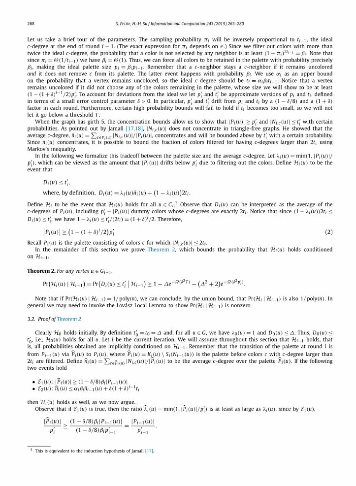

268 S. Pettie, H.-H. Su / Information and Computation 243 (2015) 263–280

Let us take a brief tour of the parameters. The sampling probability πi will be inversely proportional to ti−1, the ideal c-degree at the end of round i − 1. (The exact expression for πi depends on ε .) Since we filter out colors with more than twice the ideal c-degree, the probability that a color is not selected by any neighbor is at least (1 − πi)

2ti−1 = βi . Note that since πi = Θ(1/ti−1) we have βi = Θ(1). Thus, we can force all colors to be retained in the palette with probability precisely βi , making the ideal palette size pi = βi pi−1. Remember that a c-neighbor stays a c-neighbor if it remains uncolored and it does not remove c from its palette. The latter event happens with probability βi . We use αi as an upper bound on the probability that a vertex remains uncolored, so the ideal c-degree should be ti = αiβiti−1. Notice that a vertex remains uncolored if it did not choose any of the colors remaining in the palette, whose size we will show to be at least (1 − (1 + δ)i−1/2)p′

i . To account for deviations from the ideal we let p′i and t′

i be approximate versions of pi and ti , defined in terms of a small error control parameter δ > 0. In particular, p′

i and t′i drift from pi and ti by a (1 − δ/8) and a (1 + δ)

factor in each round. Furthermore, certain high probability bounds will fail to hold if ti becomes too small, so we will not let it go below a threshold T .

When the graph has girth 5, the concentration bounds allow us to show that |Pi(u)| ≥ p′i and |Ni,c(u)| ≤ t′

i with certain probabilities. As pointed out by Jamall [17,18], |Ni,c(u)| does not concentrate in triangle-free graphs. He showed that the average c-degree, ni(u) = ∑

c∈Pi (u) |Ni,c(u)|/|Pi(u)|, concentrates and will be bounded above by t′i with a certain probability.

Since ni(u) concentrates, it is possible to bound the fraction of colors filtered for having c-degrees larger than 2ti using Markov’s inequality.

In the following we formalize this tradeoff between the palette size and the average c-degree. Let λi (u) = min(1, |Pi(u)|/p′

i), which can be viewed as the amount that |Pi(u)| drifts below p′i due to filtering out the colors. Define Hi(u) to be the

event that

Di(u) ≤ t′i,

where, by definition, Di(u) = λi(u)ni(u) + (1 − λi(u)

)2ti .

Define Hi to be the event that Hi(u) holds for all u ∈ Gi .3 Observe that Di(u) can be interpreted as the average of the c-degrees of Pi(u), including p′

i − |Pi(u)| dummy colors whose c-degrees are exactly 2ti . Notice that since (1 − λi(u))2ti ≤Di(u) ≤ t′

i , we have 1 − λi(u) ≤ t′i/(2ti) = (1 + δ)i/2. Therefore,∣∣Pi(u)

∣∣ ≥ (1 − (1 + δ)i/2

)p′

i (2)

Recall Pi(u) is the palette consisting of colors c for which |Ni,c(u)| ≤ 2ti .In the remainder of this section we prove Theorem 2, which bounds the probability that Hi(u) holds conditioned

on Hi−1.

Theorem 2. For any vertex u ∈ Gi−1 ,

Pr(Hi(u) | Hi−1

) = Pr(

Di(u) ≤ t′i

∣∣ Hi−1) ≥ 1 − Δe−Ω(δ2 T ) − (

Δ2 + 2)e−Ω(δ2 p′

i).

Note that if Pr(Hi(u) |Hi−1) = 1/ poly(n), we can conclude, by the union bound, that Pr(Hi |Hi−1) is also 1/ poly(n). In general we may need to invoke the Lovász Local Lemma to show Pr(Hi |Hi−1) is nonzero.

3.2. Proof of Theorem 2

Clearly H0 holds initially. By definition t′0 = t0 = Δ and, for all u ∈ G , we have λ0(u) = 1 and D0(u) ≤ Δ. Thus, D0(u) ≤

t′0, i.e., H0(u) holds for all u. Let i be the current iteration. We will assume throughout this section that Hi−1 holds, that

is, all probabilities obtained are implicitly conditioned on Hi−1. Remember that the transition of the palette at round i is from Pi−1(u) via P i(u) to Pi(u), where P i(u) = Ki(u) \ Si(Ni−1(u)) is the palette before colors c with c-degree larger than 2ti are filtered. Define ni(u) = ∑

c∈ P i (u) |Ni,c(u)|/| P i(u)| to be the average c-degree over the palette P i(u). If the following two events hold

• E1(u): | P i(u)| ≥ (1 − δ/8)βi |Pi−1(u)|• E2(u): ni(u) ≤ αiβini−1(u) + δ(1 + δ)i−1ti

then Hi(u) holds as well, as we now argue.Observe that if E1(u) is true, then the ratio λi(u) = min(1, | P i(u)|/p′

i) is at least as large as λi(u), since by E1(u),

| P i(u)|p′

i

≥ (1 − δ/8)βi|Pi−1(u)|(1 − δ/8)βi p′

i−1= |Pi−1(u)|

p′i−1

.

3 This is equivalent to the induction hypothesis of Jamall [17].

S. Pettie, H.-H. Su / Information and Computation 243 (2015) 263–280 269

Therefore,

λi(u) ≥ λi(u) ≥ λi−1(u). (3)

Consider Di(u) = λi(u)ni(u) + (1 − λi(u))2ti . Compared to Di(u), Di(u) can be viewed as the average c-degree of the palette obtained by changing those colors in P i(u) whose c-degrees are greater than 2ti to dummy colors with c-degrees exactly 2ti . Since the average only goes down in this process,

Di(u) ≤ Di(u). (4)

Notice that ni−1(u) ≤ 2ti and that Hi−1 implies ni−1(u) ≤ Di−1(u) ≤ t′i−1. We will choose δ = o(1) sufficiently small so

that (1 + δ)i = 1 + o(1) for any iteration index i encountered in the algorithm. Therefore,

ni(u) ≤ αiβini−1(u) + δ(1 + δ)i−1ti by E2(u)

≤ αiβit′i−1 + δ(1 + δ)i−1ti

≤ (1 + δ)i−1ti + δ(1 + δ)i−1ti αiβiti−1 ≤ ti

= t′i ≤ 2ti (1 + δ)i = 1 + o(1) < 2 (5)

Now we have

Di(u) ≤ Di(u) by (4)

= λi(u)ni(u) + (1 − λi(u)

)2ti defn. of Di(u)

≤ λi−1(u)ni(u) + (1 − λi−1(u)

)2ti by (3) and (5)

≤ λi−1(u)(αiβini−1(u) + δ(1 + δ)i−1ti

) + (1 − λi−1(u)

)2ti by E2(u)

≤ αiβi(ni−1(u) + (

1 − λi−1(u))2ti−1

) + δ(1 + δ)i−1ti ti = αiβiti−1

≤ αiβi Di−1(u) + δ(1 + δ)i−1ti defn. of Di−1(u)

≤ αiβit′i−1 + δ(1 + δ)i−1ti Hi−1 : Di−1(u) ≤ t′

i−1

≤ (1 + δ)i−1ti + δ(1 + δ)i−1ti αiβiti−1 ≤ ti

= t′i defn. of t′

i

It remains to prove that E1(u) and E2(u) hold with sufficiently high probability.

3.3. Analysis of E1(u) and E2(u)

In this section we show that if Hi−1 holds (that is, Di−1(x) ≤ t′i−1 for all x), then events E1(u) and E2(u) only fail with

probability exponentially small in p′i and T .

The step P i(u) ← Ki(u) \ Si(Ni−1(u)) makes each color remain in P i(u) with probability exactly βi independently, there-fore E[| P i(u)|] = βi |Pi−1(u)|. By Chernoff Bound, we immediately get that E1(u) holds with the following probability:

Lemma 5. Pr(E1(u)) = Pr(| P i(u)| ≥ (1 − δ/8)βi |Pi−1(u)|) ≥ 1 − e−Ω(δ2 p′i) .

The next step is to bound the probability of E2(u). Jamall [17–19] attempted to bound ni(u) by arguing that, for each c, the value of each |Ni,c(u)| is independent of |Ni,c′ (u)| for c′ = c. Thus, the sum

∑c∈ P i−1(u) |Ni,c(u)| will concentrate. How-

ever, they are not independent since a vertex x ∈ Ni−1(u) can affect |Ni,c(u)| for all c ∈ Pi−1(x) if x becomes colored in round i.

To fix this, our idea is to break the analysis into two steps. Define the auxiliary c-neighbor set Ni,c(u) = x : x ∈Ni−1,c(u) and c ∈ P i(x) to be the set of neighbors x ∈ Ni−1,c(u) with c remaining in P i(x) regardless of whether x is colored during round i or not.

For the first step, we will show that due to the independence among |Ni,c(u)|, for each c ∈ Pi−1(u), ∑

c∈ P i (u) |Ni,c(u)|will concentrate below β2

i ni−1(u)|Pi−1(u)|. For the second step, we will calculate the probability of |Ni,c(u)| ≤ αi |Ni,c(u)|for each c ∈ Pi−1(u) individually.

Finally, by taking the union bound for the first step and the second step for all c ∈ Pi−1(u), we can prove that ∑c∈ P (u) |Ni,c(u)| concentrates below αiβ

2ni−1(u)|Pi−1(u)|, which is about αiβini−1(u)| P i(u)| by Lemma 5.

i i

270 S. Pettie, H.-H. Su / Information and Computation 243 (2015) 263–280

Lemma 6. Pr(∑

c∈ P i(u) |Ni,c(u)| ≤ β2i |Pi−1(u)|(ni−1(u) + δ

4 ti−1)) ≥ 1 − e−Ω(δ2 p′i) .

Proof. Let Yc = |Ni,c(u)| if c ∈ P i(u), and Yc = 0 otherwise. Observe that since G is triangle-free, two adjacent vertices uand x have disjoint neighborhoods. Also, whether c ∈ P i(u) only depends on the colors selected by its neighbors, not itself. Therefore, Pr(c ∈ P i(x) | c ∈ P i(u)) = βi for all c ∈ Pi−1(x). By linearity of expectation, E[Yc] = Pr(c ∈ P i(u))

∑x∈Ni−1,c(u) Pr(c ∈

P i(x) | c ∈ P i(u)) = β2i |Ni−1,c(u)|.

It is clear that ∑

c∈ P i (u) |Ni,c(u)| = ∑c∈Pi−1(u) Yc . By linearity of expectation again, we get that E[∑c∈ P i (u) |Ni,c(u)|] =

E[∑c∈Pi−1(u) Yc] = β2i ni−1(u)|Pi−1(u)|.

Since each Yc ranges from 0 to 2ti−1 and the Yc are independent, by Hoeffding’s inequality we have

Pr

( ∑c∈ P i(u)

∣∣Ni,c(u)∣∣ ≥ β2

i

∣∣Pi−1(u)∣∣(ni−1(u) + δ

4ti−1

))

= Pr

( ∑c∈ P i(u)

∣∣Ni,c(u)∣∣ ≥ E

[ ∑c∈ P i(u)

∣∣Ni,c(u)∣∣] + δ

4β2

i

∣∣Pi−1(u)∣∣ti−1

)

≤ exp

(− δ2β4

i t2i−1

∣∣Pi−1(u)∣∣2

8∑

c∈Pi−1(u)(2ti−1)2

)

≤ exp

(−δ2β4

i |Pi−1(u)|32

)

≤ exp

(−δ2β4

i (1 − (1 + δ)i−1/2)p′i−1

32

)≤ exp

(−Ω(δ2 p′

i

))by (2) and note βi = Ω(1)

Next, we are going to bound the number of uncolored neighbors in Ni,c(u) for each c ∈ Pi−1(u). Note that we are not conditioning on whether c ∈ P i(u) at this point. Instead, we will take the union bound over all c ∈ Pi−1(u) in the end so that the next lemma holds for all c ∈ Pi−1(u).

Lemma 7. Fix an iteration i, vertex u, and color c ∈ Pi−1(u). Letting M = max(αi |Ni,c(u)|, T ), then we have

Pr(∣∣Ni,c(u)

∣∣ ≤ αi∣∣Ni,c(u)

∣∣ + (δ/5)M) ≥ 1 − e−Ω(δ2 T ) − Δe−Ω(δ2 p′

i).

Proof. Let E be the event that E1(x) holds for all x ∈ Ni−1,c(u). By Lemma 5 and the union bound over each x ∈ Ni−1,c(u), Pr(E) ≤ |Ni−1,c(u)|e−Ω(δ2 p′

i) ≤ Δe−Ω(δ2 p′i) . When E occurs, for all x ∈ Ni−1,c(u), we have:∣∣ P i(x)

∣∣ ≥ (1 − δ/8)βi∣∣Pi−1(x)

∣∣ by E1(x)

≥ (1 − δ/8)βi(1 − (1 + δ)i−1/2

)p′

i−1 by (2)

= (1 − (1 + δ)i−1/2

)p′

i By defn., p′i = (1 − δ/8)βi p′

i−1

Note that the event E is determined only by the following random variables:

• Ki(x), for all x ∈ Ni−1,c(u), and• Si(w), for all w ∈ Ni−1(Ni−1,c(u)).

Therefore, we can let E = ⋃ω Eω , where the Eω represents all the possible outcomes of these random variables that

imply E . Then, Pr(|Ni,c(u)| ≤ αi |Ni,c(u)| + (δ/5)M | E) is exactly∑ω

Pr(∣∣Ni,c(u)

∣∣ ≤ αi∣∣Ni,c(u)

∣∣ + (δ/5)M∣∣ Eω

) · Pr(Eω | E)

Since ω = ω′ implies Eω ∩ Eω′ = ∅, ∑

ω Pr(Eω | E) = 1. It is sufficient to bound Pr(|Ni,c(u)| ≤ αi |Ni,c(u)| + (δ/5)M | Eω)

for each Eω . When conditioning on Eω , the neighbor set Ni,c(u) is determined and the palette P i(x) for each x ∈ Ni,c(u)

is also determined. Furthermore, since G is triangle-free, Ni−1(Ni−1,c(u)) must be disjoint from Ni,c(u). This implies that conditioning on Eω does not have any influence on Si(x) for x ∈ Ni,c(u). For all x ∈ Ni,c(u), each c ∈ P i(x) is selected with probability πi independently.

Therefore, the probability x remains uncolored conditioned on Eω , Pr(x ∈ Ni,c(u) | Eω), must be independent of all other nodes in Ni,c(u). Since x is uncolored iff x did not select any color in P i(x),

Pr(x ∈ Ni,c(u)

∣∣ Eω

) ≤ (1 − πi)| P i(x)| ≤ (1 − πi)

(1−(1+δ)i−1/2)p′i = αi .

S. Pettie, H.-H. Su / Information and Computation 243 (2015) 263–280 271

Therefore, E[Ni,c(u) | Eω] ≤ αi |Ni,c(u)|. By applying Corollary 4 with M = max(αi |Ni,c(u)|, T ) we get

Pr(∣∣Ni,c(u)

∣∣ ≤ αi∣∣Ni,c(u)

∣∣ + (δ/5)M∣∣ Eω

) ≥ 1 − e−Ω(δ2 T )

and, therefore,

Pr(∣∣Ni,c(u)

∣∣ ≤ αi∣∣Ni,c(u)

∣∣ + (δ/5)M∣∣ E) ≥ 1 − e−Ω(δ2 T ).

Since Pr(E) ≤ Δe−Ω(δ2 p′i) , by Lemma 3, we can conclude that

Pr(∣∣Ni,c(u)

∣∣ ≤ αi∣∣Ni,c(u)

∣∣ + (δ/5)M) ≥ 1 − e−Ω(δ2 T ) − Δe−Ω(δ2 p′

i). For convenience we restate Theorem 2 before proving it. Recall from Section 3.1 that Hi = ⋂

u∈GiHi(u) and Hi(u) is the

event that Di(u) ≤ t′i .

Theorem 2. For any vertex u ∈ Gi−1 ,

Pr(Hi(u)

∣∣ Hi−1) = Pr

(Di(u) ≤ t′

i

∣∣ Hi−1) ≥ 1 − Δe−Ω(δ2 T ) − (

Δ2 + 2)e−Ω(δ2 p′

i).

Proof. By Lemmas 5, 6, 7, and the union bound, the following hold with probability at least 1 − Δe−Ω(δ2 T ) − (Δ2 +2)e−Ω(δ2 p′

i) .∣∣ P i(u)∣∣ ≥ (1 − δ/8)βi

∣∣Pi−1(u)∣∣ (6)∑

c∈ P i(u)

∣∣Ni,c(u)∣∣ ≤ β2

i

∣∣Pi−1(u)∣∣(ni−1(u) + δ

4ti−1

)(7)

For all c ∈ Pi−1(u),∣∣Ni,c(u)

∣∣ ≤ αi∣∣Ni,c(u)

∣∣ + (δ/5)max(αi Ni,c(u), T

)(8)

Therefore,∑c∈ P i(u)

∣∣Ni,c(u)∣∣

≤∑

c∈ P i(u)

(αi

∣∣Ni,c(u)∣∣ + (δ/5)max

(αi

∣∣Ni,c(u)∣∣, T

))by (8)

≤ (1 + δ/5)αi

( ∑c∈ P i(u)

∣∣Ni,c(u)∣∣) + (δ/5)

∣∣ P i(u)∣∣T max(a,b) ≤ a + b

≤ βi∣∣Pi−1(u)

∣∣(1 + δ/5)

(αiβini−1(u) + δ

4αiβiti−1

)+ (δ/5)

∣∣ P i(u)∣∣T by (7)

≤ 1 + δ/5

1 − δ/8

∣∣ P i(u)∣∣(αiβini−1(u) + δ

4αiβiti−1

)+ (δ/5)

∣∣ P i(u)∣∣T by (6)

Therefore,

ni(u) =∑

c∈ P i(u)

∣∣Ni,c(u)∣∣/∣∣ P i(u)

∣∣≤ 1 + δ/5

1 − δ/8

(αiβini−1(u) + (δ/4)αiβiti−1

) + (δ/5)T

≤ (1 + δ/2)(αiβini−1(u) + (δ/4)αiβit

′i−1

) + (δ/5)T when δ < 1

≤ (1 + δ/2)(αiβini−1(u) + (δ/4)αiβit

′i−1

) + (δ/5)ti T ≤ ti

≤ αiβini−1(u) + (δ/2 + δ/4 + δ2/8

)αiβit

′i−1 + (δ/5)ti ni−1(u) ≤ t′

i−1

≤ αiβini−1(u) + (δ/2 + δ/4 + δ2/8 + δ/5

)(1 + δ)i−1ti αiβit

′i−1 = ti(1 + δ)i−1

≤ αiβini−1(u) + δ(1 + δ)i−1ti when δ ≤ 2/5

As we showed in Section 3.2, whenever E1(u) and E2(u) hold, Hi(u) holds as well.

272 S. Pettie, H.-H. Su / Information and Computation 243 (2015) 263–280

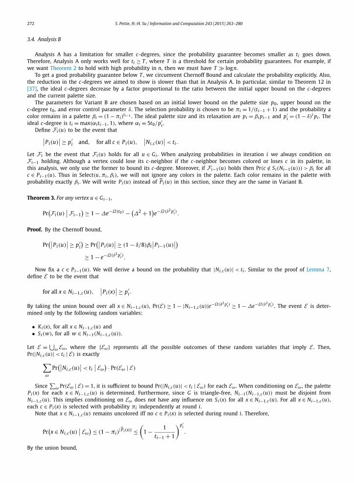
3.4. Analysis B

Analysis A has a limitation for smaller c-degrees, since the probability guarantee becomes smaller as ti goes down. Therefore, Analysis A only works well for ti ≥ T , where T is a threshold for certain probability guarantees. For example, if we want Theorem 2 to hold with high probability in n, then we must have T log n.

To get a good probability guarantee below T , we circumvent Chernoff Bound and calculate the probability explicitly. Also, the reduction in the c-degrees we aimed to show is slower than that in Analysis A. In particular, similar to Theorem 12 in [37], the ideal c-degrees decrease by a factor proportional to the ratio between the initial upper bound on the c-degrees and the current palette size.

The parameters for Variant B are chosen based on an initial lower bound on the palette size p0, upper bound on the c-degree t0, and error control parameter δ. The selection probability is chosen to be πi = 1/(ti−1 + 1) and the probability a color remains in a palette βi = (1 − πi)

ti−1 . The ideal palette size and its relaxation are pi = βi pi−1 and p′i = (1 − δ)i pi . The

ideal c-degree is ti = max(αiti−1, 1), where αi = 5t0/p′i .

Define Fi(u) to be the event that∣∣Pi(u)∣∣ ≥ p′

i and, for all c ∈ Pi(u),∣∣Ni,c(u)

∣∣ < ti .

Let Fi be the event that Fi(u) holds for all u ∈ Gi . When analyzing probabilities in iteration i we always condition on Fi−1 holding. Although a vertex could lose its c-neighbor if the c-neighbor becomes colored or loses c in its palette, in this analysis, we only use the former to bound its c-degree. Moreover, if Fi−1(u) holds then Pr(c /∈ Si(Ni−1(u))) > βi for all c ∈ Pi−1(u). Thus in Select(u, πi, βi), we will not ignore any colors in the palette. Each color remains in the palette with probability exactly βi . We will write Pi(u) instead of P i(u) in this section, since they are the same in Variant B.

Theorem 3. For any vertex u ∈ Gi−1 ,

Pr(Fi(u)

∣∣ Fi−1) ≥ 1 − Δe−Ω(t0) − (

Δ2 + 1)e−Ω(δ2 p′

i).

Proof. By the Chernoff bound,

Pr(∣∣Pi(u)

∣∣ ≥ p′i

) ≥ Pr(∣∣Pi(u)

∣∣ ≥ (1 − δ/8)βi∣∣Pi−1(u)

∣∣)≥ 1 − e−Ω(δ2 p′

i).

Now fix a c ∈ Pi−1(u). We will derive a bound on the probability that |Ni,c(u)| < ti . Similar to the proof of Lemma 7, define E to be the event that

for all x ∈ Ni−1,c(u),∣∣Pi(x)

∣∣ ≥ p′i .

By taking the union bound over all x ∈ Ni−1,c(u), Pr(E) ≥ 1 − |Ni−1,c(u)|e−Ω(δ2 p′i) ≥ 1 − Δe−Ω(δ2 p′

i) . The event E is deter-mined only by the following random variables:

• Ki(x), for all x ∈ Ni−1,c(u) and• Si(w), for all w ∈ Ni−1(Ni−1,c(u)).

Let E = ⋃ω Eω , where the Eω represents all the possible outcomes of these random variables that imply E . Then,

Pr(|Ni,c(u)| < ti | E) is exactly∑ω

Pr(∣∣Ni,c(u)

∣∣ < ti∣∣ Eω

) · Pr(Eω | E)

Since ∑

ω Pr(Eω | E) = 1, it is sufficient to bound Pr(|Ni,c(u)| < ti | Eω) for each Eω . When conditioning on Eω , the palette Pi(x) for each x ∈ Ni−1,c(u) is determined. Furthermore, since G is triangle-free, Ni−1(Ni−1,c(u)) must be disjoint from Ni−1,c(u). This implies conditioning on Eω does not have any influence on Si(x) for all x ∈ Ni−1,c(u). For all x ∈ Ni−1,c(u), each c ∈ Pi(x) is selected with probability πi independently at round i.

Note that x ∈ Ni−1,c(u) remains uncolored iff no c ∈ Pi(x) is selected during round i. Therefore,

Pr(x ∈ Ni,c(u)

∣∣ Eω

) ≤ (1 − πi)| P i(x)| ≤

(1 − 1

ti−1 + 1

)p′i

.

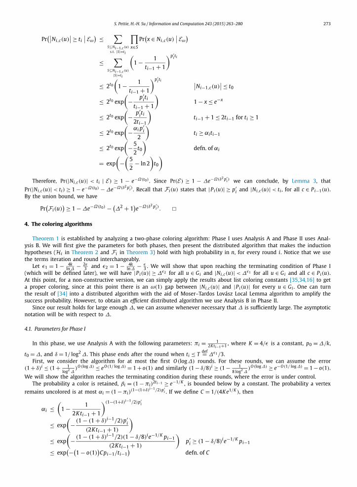
By the union bound,

S. Pettie, H.-H. Su / Information and Computation 243 (2015) 263–280 273

Pr(∣∣Ni,c(u)

∣∣ ≥ ti∣∣ Eω

) ≤∑

S⊆Ni−1,c (u)

s.t. |S|=ti

∏x∈S

Pr(x ∈ Ni,c(u)

∣∣ Eω

)

≤∑

S⊆Ni−1,c (u)

|S|=ti

(1 − 1

ti−1 + 1

)p′i ti

≤ 2t0

(1 − 1

ti−1 + 1

)p′i ti ∣∣Ni−1,c(u)

∣∣ ≤ t0

≤ 2t0 exp

(− p′

iti

ti−1 + 1

)1 − x ≤ e−x

≤ 2t0 exp

(− p′

iti

2ti−1

)ti−1 + 1 ≤ 2ti−1 for ti ≥ 1

≤ 2t0 exp

(−αi p′

i

2

)ti ≥ αiti−1

≤ 2t0 exp

(−5

2t0

)defn. of αi

= exp

(−

(5

2− ln 2

)t0

)

Therefore, Pr(|Ni,c(u)| < ti | E) ≥ 1 − e−Ω(t0) . Since Pr(E) ≥ 1 − Δe−Ω(δ2 p′i) we can conclude, by Lemma 3, that

Pr(|Ni,c(u)| < ti) ≥ 1 − e−Ω(t0) − Δe−Ω(δ2 p′i) . Recall that Fi(u) states that |Pi(u)| ≥ p′

i and |Ni,c(u)| < ti , for all c ∈ Pi−1(u). By the union bound, we have

Pr(Fi(u)

) ≥ 1 − Δe−Ω(t0) − (Δ2 + 1

)e−Ω(δ2 p′

i). 4. The coloring algorithms

Theorem 1 is established by analyzing a two-phase coloring algorithm: Phase I uses Analysis A and Phase II uses Anal-ysis B. We will first give the parameters for both phases, then present the distributed algorithm that makes the induction hypotheses (Hi in Theorem 2 and Fi in Theorem 3) hold with high probability in n, for every round i. Notice that we use the terms iteration and round interchangeably.

Let ε1 = 1 − 4kln Δ

− 2ε3 and ε2 = 1 − 4k

ln Δ− ε

3 . We will show that upon reaching the terminating condition of Phase I (which will be defined later), we will have |Pi(u)| ≥ Δε2 for all u ∈ Gi and |Ni,c(u)| < Δε1 for all u ∈ Gi and all c ∈ Pi(u). At this point, for a non-constructive version, we can simply apply the results about list coloring constants [35,34,16] to get a proper coloring, since at this point there is an ω(1) gap between |Ni,c(u)| and |Pi(u)| for every u ∈ Gi . One can turn the result of [34] into a distributed algorithm with the aid of Moser–Tardos Lovász Local Lemma algorithm to amplify the success probability. However, to obtain an efficient distributed algorithm we use Analysis B in Phase II.

Since our result holds for large enough Δ, we can assume whenever necessary that Δ is sufficiently large. The asymptotic notation will be with respect to Δ.

4.1. Parameters for Phase I

In this phase, we use Analysis A with the following parameters: πi = 12Kti−1+1 , where K = 4/ε is a constant, p0 = Δ/k,

t0 = Δ, and δ = 1/ log2 Δ. This phase ends after the round when ti ≤ Tdef= Δε1/3.

First, we consider the algorithm for at most the first O (logΔ) rounds. For these rounds, we can assume the error (1 + δ)i ≤ (1 + 1

log2 Δ)O (log Δ) ≤ eO (1/ log Δ) = 1 + o(1) and similarly (1 − δ/8)i ≥ (1 − 1

8 log2 Δ)O (log Δ) ≥ e−O (1/ log Δ) = 1 − o(1).

We will show the algorithm reaches the terminating condition during these rounds, where the error is under control.The probability a color is retained, βi = (1 − πi)

2ti−1 ≥ e−1/K , is bounded below by a constant. The probability a vertex remains uncolored is at most αi = (1 − πi)

(1−(1+δ)i−1/2)p′i . If we define C = 1/(4K e1/K ), then

αi ≤(

1 − 1

2Kti−1 + 1

)(1−(1+δ)i−1/2)p′i

≤ exp

(− (1 − (1 + δ)i−1/2)p′

i

(2Kti−1 + 1)

)

≤ exp

(− (1 − (1 + δ)i−1/2)(1 − δ/8)ie−1/K pi−1

(2Kti−1 + 1)

)p′

i ≥ (1 − δ/8)ie−1/K pi−1

≤ exp(−(

1 − o(1))Cp /t

)defn. of C

i−1 i−1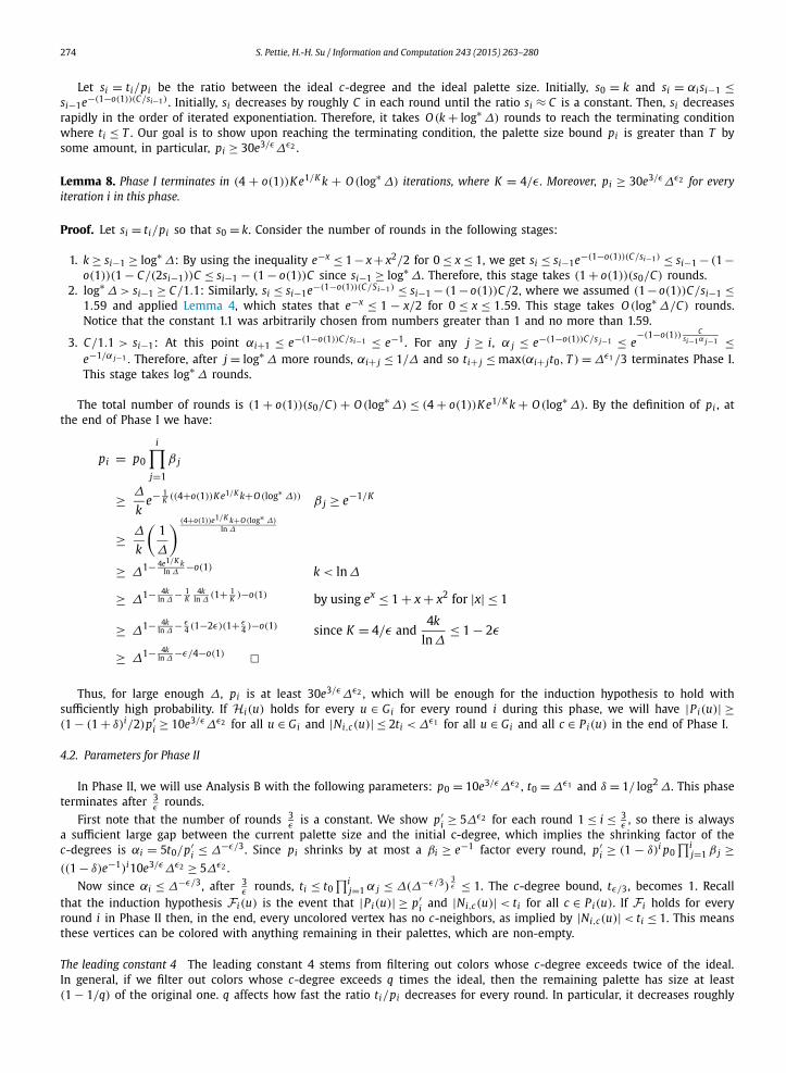

274 S. Pettie, H.-H. Su / Information and Computation 243 (2015) 263–280

Let si = ti/pi be the ratio between the ideal c-degree and the ideal palette size. Initially, s0 = k and si = αi si−1 ≤si−1e−(1−o(1))(C/si−1) . Initially, si decreases by roughly C in each round until the ratio si ≈ C is a constant. Then, si decreases rapidly in the order of iterated exponentiation. Therefore, it takes O (k + log∗ Δ) rounds to reach the terminating condition where ti ≤ T . Our goal is to show upon reaching the terminating condition, the palette size bound pi is greater than T by some amount, in particular, pi ≥ 30e3/εΔε2 .

Lemma 8. Phase I terminates in (4 + o(1))K e1/K k + O (log∗ Δ) iterations, where K = 4/ε . Moreover, pi ≥ 30e3/εΔε2 for every iteration i in this phase.

Proof. Let si = ti/pi so that s0 = k. Consider the number of rounds in the following stages:

1. k ≥ si−1 ≥ log∗ Δ: By using the inequality e−x ≤ 1 − x + x2/2 for 0 ≤ x ≤ 1, we get si ≤ si−1e−(1−o(1))(C/si−1) ≤ si−1 − (1 −o(1))(1 − C/(2si−1))C ≤ si−1 − (1 − o(1))C since si−1 ≥ log∗ Δ. Therefore, this stage takes (1 + o(1))(s0/C) rounds.

2. log∗ Δ > si−1 ≥ C/1.1: Similarly, si ≤ si−1e−(1−o(1))(C/Si−1) ≤ si−1 − (1 −o(1))C/2, where we assumed (1 −o(1))C/si−1 ≤1.59 and applied Lemma 4, which states that e−x ≤ 1 − x/2 for 0 ≤ x ≤ 1.59. This stage takes O (log∗ Δ/C) rounds. Notice that the constant 1.1 was arbitrarily chosen from numbers greater than 1 and no more than 1.59.

3. C/1.1 > si−1: At this point αi+1 ≤ e−(1−o(1))C/si−1 ≤ e−1. For any j ≥ i, α j ≤ e−(1−o(1))C/s j−1 ≤ e−(1−o(1)) C

si−1α j−1 ≤e−1/α j−1 . Therefore, after j = log∗ Δ more rounds, αi+ j ≤ 1/Δ and so ti+ j ≤ max(αi+ jt0, T ) = Δε1/3 terminates Phase I. This stage takes log∗ Δ rounds.

The total number of rounds is (1 + o(1))(s0/C) + O (log∗ Δ) ≤ (4 + o(1))K e1/K k + O (log∗ Δ). By the definition of pi , at the end of Phase I we have:

pi = p0

i∏j=1

β j

≥ Δ

ke− 1

K ((4+o(1))K e1/K k+O (log∗ Δ)) β j ≥ e−1/K

≥ Δ

k

(1

Δ

) (4+o(1))e1/K k+O (log∗ Δ)ln Δ

≥ Δ1− 4e1/K kln Δ

−o(1) k < lnΔ

≥ Δ1− 4kln Δ

− 1K

4kln Δ

(1+ 1K )−o(1) by using ex ≤ 1 + x + x2 for |x| ≤ 1

≥ Δ1− 4kln Δ

− ε4 (1−2ε)(1+ ε

4 )−o(1) since K = 4/ε and4k

lnΔ≤ 1 − 2ε

≥ Δ1− 4kln Δ

−ε/4−o(1) Thus, for large enough Δ, pi is at least 30e3/εΔε2 , which will be enough for the induction hypothesis to hold with

sufficiently high probability. If Hi(u) holds for every u ∈ Gi for every round i during this phase, we will have |Pi(u)| ≥(1 − (1 + δ)i/2)p′

i ≥ 10e3/εΔε2 for all u ∈ Gi and |Ni,c(u)| ≤ 2ti < Δε1 for all u ∈ Gi and all c ∈ Pi(u) in the end of Phase I.

4.2. Parameters for Phase II

In Phase II, we will use Analysis B with the following parameters: p0 = 10e3/εΔε2 , t0 = Δε1 and δ = 1/ log2 Δ. This phase terminates after 3

ε rounds.

First note that the number of rounds 3ε is a constant. We show p′

i ≥ 5Δε2 for each round 1 ≤ i ≤ 3ε , so there is always

a sufficient large gap between the current palette size and the initial c-degree, which implies the shrinking factor of the c-degrees is αi = 5t0/p′

i ≤ Δ−ε/3. Since pi shrinks by at most a βi ≥ e−1 factor every round, p′i ≥ (1 − δ)i p0

∏ij=1 β j ≥

((1 − δ)e−1)i10e3/εΔε2 ≥ 5Δε2 .

Now since αi ≤ Δ−ε/3, after 3ε rounds, ti ≤ t0

∏ij=1 α j ≤ Δ(Δ−ε/3)

3ε ≤ 1. The c-degree bound, tε/3, becomes 1. Recall

that the induction hypothesis Fi(u) is the event that |Pi(u)| ≥ p′i and |Ni,c(u)| < ti for all c ∈ Pi(u). If Fi holds for every

round i in Phase II then, in the end, every uncolored vertex has no c-neighbors, as implied by |Ni,c(u)| < ti ≤ 1. This means these vertices can be colored with anything remaining in their palettes, which are non-empty.

The leading constant 4 The leading constant 4 stems from filtering out colors whose c-degree exceeds twice of the ideal. In general, if we filter out colors whose c-degree exceeds q times the ideal, then the remaining palette has size at least (1 − 1/q) of the original one. q affects how fast the ratio ti/pi decreases for every round. In particular, it decreases roughly

S. Pettie, H.-H. Su / Information and Computation 243 (2015) 263–280 275

by 1/(q/(1 − 1/q)K e1/K ) for every round. Note that the palette size decreases by a fixed rate βi ∼ e1/K for each round i and we have to keep it large enough as stated in Lemma 8 (pi ≥ 30e3/εΔε2 ). Given that the number of rounds we allow is fixed, the leading constant we can get depends on how fast the ratio ti/pi decreases. Therefore, we choose q = 2 to maximize 1/(q/(1 − 1/q)K e1/K ), which results in a leading constant of 4.

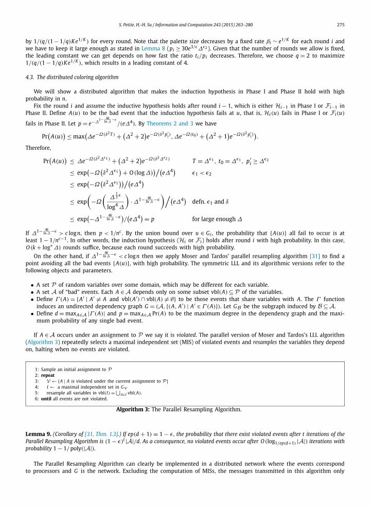
4.3. The distributed coloring algorithm

We will show a distributed algorithm that makes the induction hypothesis in Phase I and Phase II hold with high probability in n.

Fix the round i and assume the inductive hypothesis holds after round i − 1, which is either Hi−1 in Phase I or Fi−1 in Phase II. Define A(u) to be the bad event that the induction hypothesis fails at u, that is, Hi(u) fails in Phase I or Fi(u)

fails in Phase II. Let p = e−Δ1− 4k

ln Δ−ε

/(eΔ4). By Theorems 2 and 3 we have

Pr(

A(u)) ≤ max

(Δe−Ω(δ2 T ) + (

Δ2 + 2)e−Ω(δ2 p′

i),Δe−Ω(t0) + (Δ2 + 1

)e−Ω(δ2 p′

i)).

Therefore,

Pr(

A(u)) ≤ Δe−Ω(δ2Δε1 ) + (

Δ2 + 2)e−Ω(δ2Δε2 ) T = Δε1 , t0 = Δε1 , p′

i ≥ Δε2

≤ exp(−Ω

(δ2Δε1

) + O (log Δ))/(

eΔ4) ε1 < ε2

≤ exp(−Ω

(δ2Δε1

))/(eΔ4)

≤ exp

(−Ω

(Δ

13 ε

log4 Δ

)· Δ1− 4k

ln Δ−ε

)/(eΔ4) defn. ε1 and δ

≤ exp(−Δ1− 4k

ln Δ−ε

)/(eΔ4) = p for large enough Δ

If Δ1− 4kln Δ

−ε > c log n, then p < 1/nc . By the union bound over u ∈ Gi , the probability that A(u) all fail to occur is at least 1 − 1/nc−1. In other words, the induction hypothesis (Hi or Fi) holds after round i with high probability. In this case, O (k + log∗ Δ) rounds suffice, because each round succeeds with high probability.

On the other hand, if Δ1− 4kln Δ

−ε < c log n then we apply Moser and Tardos’ parallel resampling algorithm [31] to find a point avoiding all the bad events A(u), with high probability. The symmetric LLL and its algorithmic versions refer to the following objects and parameters.

• A set P of random variables over some domain, which may be different for each variable.• A set A of “bad” events. Each A ∈A depends only on some subset vbl(A) ⊆P of the variables.• Define Γ (A) = A′ | A′ = A and vbl(A′) ∩ vbl(A) = ∅ to be those events that share variables with A. The Γ function

induces an undirected dependency graph G = (A, (A, A′) | A′ ∈ Γ (A)). Let GB be the subgraph induced by B ⊆A.• Define d = maxA∈A |Γ (A)| and p = maxA∈A Pr(A) to be the maximum degree in the dependency graph and the maxi-

mum probability of any single bad event.

If A ∈A occurs under an assignment to P we say it is violated. The parallel version of Moser and Tardos’s LLL algorithm (Algorithm 3) repeatedly selects a maximal independent set (MIS) of violated events and resamples the variables they depend on, halting when no events are violated.

1: Sample an initial assignment to P2: repeat3: V ← A | A is violated under the current assignment to P4: I ← a maximal independent set in GV5: resample all variables in vbl(I) = ⋃

A∈I vbl(A).6: until all events are not violated.

Algorithm 3: The Parallel Resampling Algorithm.

Lemma 9. (Corollary of [31, Thm. 1.3].) If ep(d + 1) = 1 − ε , the probability that there exist violated events after t iterations of the Parallel Resampling Algorithm is (1 − ε)t |A|/d. As a consequence, no violated events occur after O (log1/ep(d+1) |A|) iterations with probability 1 − 1/ poly(|A|).

The Parallel Resampling Algorithm can clearly be implemented in a distributed network where the events correspond to processors and G is the network. Excluding the computation of MISs, the messages transmitted in this algorithm only

276 S. Pettie, H.-H. Su / Information and Computation 243 (2015) 263–280

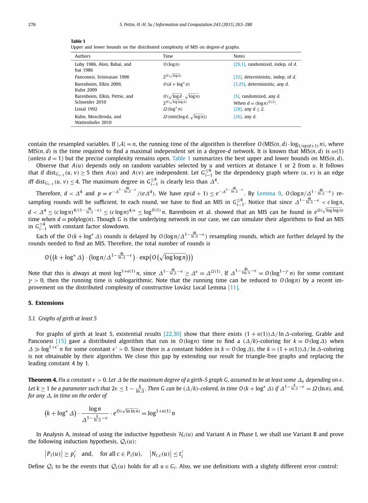
Table 1Upper and lower bounds on the distributed complexity of MIS on degree-d graphs.

Authors Time Notes

Luby 1986, Alon, Babai, and Itai 1986

O (logn) [29,1], randomized, indep. of d.

Panconesi, Srinivasan 1996 2O (√

log n) [32], deterministic, indep. of d.

Barenboim, Elkin 2009, Kuhn 2009

O (d + log∗ n) [3,25], deterministic, any d.

Barenboim, Elkin, Pettie, and Schneider 2010

O (√

log d · √log n) [5], randomized, any d.

2O (√

log log n) When d = (logn)O (1) .Linial 1992 Ω(log∗ n) [28], any d ≥ 2.

Kuhn, Moscibroda, and Wattenhofer 2010

Ω(minlog d,√

log n) [26], any d.

contain the resampled variables. If |A| = n, the running time of the algorithm is therefore O (MIS(n, d) · log1/ep(d+1) n), where MIS(n, d) is the time required to find a maximal independent set in a degree-d network. It is known that MIS(n, d) is ω(1)

(unless d = 1) but the precise complexity remains open. Table 1 summarizes the best upper and lower bounds on MIS(n, d).Observe that A(u) depends only on random variables selected by u and vertices at distance 1 or 2 from u. It follows

that if distGi−1 (u, v) ≥ 5 then A(u) and A(v) are independent. Let G≤4i−1 be the dependency graph where (u, v) is an edge

iff distGi−1 (u, v) ≤ 4. The maximum degree in G≤4i−1 is clearly less than Δ4.

Therefore, d < Δ4 and p = e−Δ1− 4k

ln Δ−ε

/(eΔ4). We have ep(d + 1) ≤ e−Δ1− 4k

ln Δ−ε

. By Lemma 9, O (log n/Δ1− 4kln Δ

−ε) re-

sampling rounds will be sufficient. In each round, we have to find an MIS in G≤4i−1. Notice that since Δ1− 4k

ln Δ−ε < c log n,

d < Δ4 ≤ (c log n)4/(1− 4kln Δ

−ε) ≤ (c log n)4/ε ≤ logO (1) n. Barenboim et al. showed that an MIS can be found in eO (√

log log n)

time when d = polylog(n). Though G is the underlying network in our case, we can simulate their algorithms to find an MIS in G≤4

i−1 with constant factor slowdown.

Each of the O (k + log∗ Δ) rounds is delayed by O (log n/Δ1− 4kln Δ

−ε) resampling rounds, which are further delayed by the rounds needed to find an MIS. Therefore, the total number of rounds is

O((

k + log∗ Δ) · (logn/Δ1− 4k

ln Δ−ε

) · exp(

O(√

log log n)))

Note that this is always at most log1+o(1) n, since Δ1− 4kln Δ

−ε ≥ Δε = ΔΩ(1) . If Δ1− 4klog Δ

−ε = O (log1−γ n) for some constant γ > 0, then the running time is sublogarithmic. Note that the running time can be reduced to O (log n) by a recent im-provement on the distributed complexity of constructive Lovász Local Lemma [11].

5. Extensions

5.1. Graphs of girth at least 5

For graphs of girth at least 5, existential results [22,30] show that there exists (1 + o(1))Δ/ ln Δ-coloring. Grable and Panconesi [15] gave a distributed algorithm that run in O (log n) time to find a (Δ/k)-coloring for k = O (log Δ) when Δ log1+ε′

n for some constant ε′ > 0. Since there is a constant hidden in k = O (logΔ), the k = (1 + o(1))Δ/ ln Δ-coloring is not obtainable by their algorithm. We close this gap by extending our result for triangle-free graphs and replacing the leading constant 4 by 1.

Theorem 4. Fix a constant ε > 0. Let Δ be the maximum degree of a girth-5 graph G, assumed to be at least some Δε depending on ε . Let k ≥ 1 be a parameter such that 2ε ≤ 1 − k

ln Δ. Then G can be (Δ/k)-colored, in time O (k + log∗ Δ) if Δ1− k

ln Δ−ε = Ω(ln n), and,

for any Δ, in time on the order of

(k + log∗ Δ

) · logn

Δ1− kln Δ

−ε· eO (

√ln ln n) = log1+o(1) n

In Analysis A, instead of using the inductive hypothesis Hi(u) and Variant A in Phase I, we shall use Variant B and prove the following induction hypothesis, Qi(u):∣∣Pi(u)

∣∣ ≥ p′i and, for all c ∈ Pi(u),

∣∣Ni,c(u)∣∣ ≤ t′

i

Define Qi to be the events that Qi(u) holds for all u ∈ Gi . Also, we use definitions with a slightly different error control:

S. Pettie, H.-H. Su / Information and Computation 243 (2015) 263–280 277

βi = (1 − πi)t′i−1 αi = (1 − πi)

p′i

pi = βi pi−1 ti = max(αiβiti−1, T )

p′i = (1 − δ)i pi t′

i = (1+δ)i∏ik=1(1−πk)

ti (9)

We use πi = 1/(1 + Kt′i) as the sampling probability in the ith iteration, where K = 4/ε . As a consequence βi is lower

bounded by a constant since

βi = (1 − πi)t′i−1 =

(1 − 1

1 + Kt′i

)t′i−1

>

(1 − 1

1 + Kt′i

)t′i> e−1/K .

Notice that since δ = 1/ log2 Δ, for the first i = O (log Δ) rounds we have p′i = pi(1 − δ)i = (1 − o(1))pi . If we choose

ε1 = 1 − kln Δ

− 2ε3 and ε2 = 1 − k

ln Δ− ε

3 , and end the phase after the first round i when ti ≤ Tdef= Δε1/3, then

t′i = (1 + δ)i∏i

k=1(1 − πk)· ti ≤

((1 + δ)

1 − (1 + KΔε1/3)−1

)i

ti ≤ (1 + o(1)

)ti .

Then, Lemma 8 holds similarly except that the algorithm runs in (1 + o(1))K e1/K k + O (log∗ Δ) time. Also, one can prove pi ≥ 30e3/εΔε2 as in the proof of Lemma 8. The argument for Phase II afterwards will be the same with that in triangle-free graphs.

The remaining task is to bound the failure probability of Qi(u), when Qi−1 holds. To show this, notice that it is possible to bound individual c-degrees rather than bounding the average c-degree in graphs of girth at least 5, since the probability a color remains in each neighbor has only a weak correlation. Instead of proving Lemma 6, we prove the following:

Lemma 10. Let β ′i = βi

(1−πi). If Qi−1 holds, then Pr(|Ni,c(u)| ≤ (1 + δ/4)β ′

i t′i−1) ≥ 1 − e−Ω(δ2 T ) .

Proof. Let x ∈ Ni−1,c(u). Whether x loses c in its palette depends on whether x’s neighbors chose c. Since G is a graph with girth at least 5, u is the only common neighbor of vertices in Ni−1,c(u). The probability that x loses c is almost independent among other vertices in Ni−1,c(u). Let Ix be the indicator random variable that c ∈ K (x) and all of x’s neighbors excluding u did not choose c (i.e. c ∈ K (x) \ Si(Ni−1,c(x) \ u)). Clearly, Ix are independent among all x ∈ Ni−1,c(u) and Pr(Ix) = β ′

i . Letting I = ∑

x Ix , we have |Ni,c(u)| ≤ I and E[I] = β ′i |Ni−1,c(u)|. Therefore,

Pr(∣∣Ni,c(u)

∣∣ ≤ (1 + δ/4)β ′i t

′i−1

)≥ Pr

(I ≤ (1 + δ/4)β ′

i t′i−1

) ∣∣Ni,c(u)∣∣ ≤ I

≥ Pr(

I ≤ E[I] + (δ/4)β ′i t

′i−1

)E[I] = β ′

i

∣∣Ni−1,c(u)∣∣ ≤ β ′

i t′i−1

≥ 1 − e−Ω(δ2β ′i t

′i−1) β ′

i t′i−1 ≥ E[I] and by Corollary 4

= 1 − e−Ω(δ2 T ) β ′i = Ω(1) and t′

i−1 ≥ T Combined with Lemma 7, we get the following:

Collorary 5. If Qi−1 holds, then Pr(∀c ∈ Pi−1(u), |Ni,c(u)| ≤ t′i) ≥ 1 − 2Δe−Ω(δ2 T ) − Δ2e−Ω(δ2 p′

i) .

Proof. By applying union bound with Lemma 10 and Lemma 7 for all c ∈ Pi−1(u), the following holds with probability at least 1 − 2Δe−Ω(δ2 T ) − Δ2e−Ω(δ2 p′

i):

1. |Ni,c(u)| ≤ (1 + δ/4)β ′i t

′i−1

2. |Ni,c(u)| ≤ αi |Ni,c(u)| + (δ/5) max(αi |Ni,c(u)|, T )

Then, we have:∣∣Ni,c(u)∣∣ ≤ αiβ

′i (1 + δ/4)(1 + δ/5)t′

i−1 + (δ/5)T max(a,b) ≤ a + b

≤ αiβ′i (1 + δ/4)(1 + 2δ/5)t′

i−1 T ≤ ti ≤ αiβiti−1 ≤ αiβ′i (1 + δ/4)ti−1

≤ (1 + δ)αiβ′i t

′i−1 δ ≤ 1

= t′i defn. of β ′

i and t′i

278 S. Pettie, H.-H. Su / Information and Computation 243 (2015) 263–280

Theorem 5. For any vertex u ∈ Gi−1 , Pr(Qi(u) |Qi−1) ≥ 1 − 2Δe−Ω(δ2 T ) − (Δ2 + 1)e−Ω(δ2 p′i) .

Proof. By Chernoff bound, we can get that Pr(|Pi(u)| ≥ p′i) = Pr(|Pi(u)| ≥ (1 − δ)βi p′

i−1) ≥ Pr(|Pi(u)| ≥ (1 − δ)βi |Pi−1(u)|) ≥1 − e−Ω(δ2 p′

i) . By the union bound and Corollary 5, we get that |Pi(u)| ≥ p′i and |Ni,c(u)| ≤ t′

i−1 for all c ∈ Pi(u) hold with probability at least 1 − 2Δe−Ω(δ2 T ) − (Δ2 + 1)e−Ω(δ2 p′

i) . Since pi ≥ C2Δ

ε2 and T = Δε1/3, the probability Qi(u) fails for u, 2Δe−Ω(δ2 T ) + (Δ2 + 1)e−Ω(δ2 p′i) , is bounded by

e−Δ1− k

ln Δ−ε

/(eΔ4) for large enough Δ. As in Section 4, depending on how small this probability is, one can either apply the union bounds to get a high success probability or use Moser and Tardos’ resampling algorithm for the Lovász Local Lemma.

5.2. Trees

Trees are graphs of infinity girth. According to Theorem 4, it is possible to get a (Δ/k)-coloring in O (k + log∗ Δ) time if Δ1− k

ln Δ−ε = Ω(log n) and ε is a constant less than or equal to 1

2 · (1 − kln Δ

). If Δ1− kln Δ

−ε = O (log n), we will show that using additional O (q) colors, it is possible to get a (Δ/k + O (q))-coloring in O (k + log∗ n + log log n

log q ) time. In any case, we can find a (1 + o(1))Δ/ ln Δ-coloring in O (logΔ + logΔ log n) rounds by choosing q = √

Δ and k = ln Δ/(1 + o(1)).The algorithm is the same with the framework of Section 5.1, except that at the end of each round we delete the bad

vertices, which are the vertices that fail to satisfy the induction hypothesis (i.e. Qi(u) in Phase I or Fi(u) in Phase II). The remaining vertices must satisfy the induction hypothesis. Using the idea from [5,6,36], we will show that after O (k + log∗ Δ)

rounds of the algorithm, the size of each component formed by the bad vertices is at most O (Δ4 log n) with high probability.Barenboim and Elkin’s deterministic algorithm [4] obtains an O (q)-coloring in O (

log nlog q + log∗ n) time for trees (arboricity

= 1). We then apply their algorithm on each component formed by bad vertices. Since the size of each component is at most O (Δ4 log n), their algorithm will run in O (

log log n+log Δlog q + log∗ n) time, using the additional O (q) colors. Note that this

running time is actually O (log log n

log q + log∗ n), since Δ = O (log1/(1− kln Δ

−ε) n) = O (log1/ε n) = logO (1) n.Define Ai(u) be the event the induction hypothesis fails at u in round i (Qi(u) fails in Phase I or Fi(u) fails in

Phase II). Since k < ln Δ, there exists a constant c1 > 0 such that the algorithm always finishes in c1 ln Δ rounds. Let p = 1/(2c1eΔ5 ln Δ). By Theorem 3 and Theorem 5 and since T ≥ Δ1− k

ln Δ− 2ε

3 and p′i ≥ Δ1− k

ln Δ− ε

3 , we have that for large enough Δ,

Pr(

Ai(u)) ≤ 2Δe−Ω(δ2 T ) + (

Δ2 + 1)e−Ω(δ2 p′

i) ≤ 1/(2c1eΔ5 lnΔ

) = p

Also note that for u, v ∈ Gi−1, Ai(u) and Ai(v) are independent if distGi−1 (u, v) ≥ 5, since Ai(u) only depends on vari-ables within distance two from u.

Lemma 11. Let H ⊆ Gi−1 be a connected component with s vertices. There exists a vertex set V 0 ⊆ H such that |V 0| = s/Δ4 and for any u, v ∈ V 0 , distGi−1 (u, v) ≥ 5 and distGi−1 (u, V 0 \ u) = 5.

Proof. Define B(v, i) = u ∈ H | distGi−1 (v, u) ≤ i. Start with an arbitrary vertex v ∈ H . Put v in V 0 and delete B(v, 4)

from H . Select a new vertex v ′ from the remaining vertices in H such that dist(v ′, V 0) = 5. If the remaining graph is non-empty, then such v ′ must exist, because H is connected. Repeat this procedure until there are s/Δ4 vertices in V 0. Since we delete at most Δ4 vertices in each iteration, the remaining graph will be non-empty until we find s/Δ4vertices.

Suppose that there exists a component H containing s bad vertices in the end of the algorithm. Let t = s/Δ4, we can extract such a subset V 0 ⊆ H with the property stated in Lemma 11. We will show that the total possible number of such V 0 will be bounded.

For any V 0, we can map it to a tree with size t in the graph G5i−1. This is because the vertex set of V 0 is connected

in G5i−1 and we can take any spanning tree of it. The mapping is injective. Therefore, the total number of possible V 0 is

at most the total possible number of ways to embed an unordered, rooted tree of t vertices in G5i−1, which is bounded by

netΔ5t [23, p. 397, Exercise 11].On the other hand, the total possible number schedules for when these t vertices become bad is at most ct

1 lnt Δ, since each vertex becomes bad in one of at most c1 ln Δ rounds in our algorithm. For those u ∈ V 0 who become bad at round i, each failure happens with probability at most p independently. Therefore,

Pr(∃H s.t. |H| ≥ s and v is bad,∀v ∈ H

)≤

∑tree T ⊆G5

i−14

Pr(v is bad, ∀v ∈ T )

|T |=s/Δ

S. Pettie, H.-H. Su / Information and Computation 243 (2015) 263–280 279

≤∑

tree T ⊆G5i−1

|T |=s/Δ4

∑B1,...,Bc1 ln Δ⊆T⋃

Bi=T ,Bi∩B j=∅

∏i

Pr(Bi become bad at round i)

≤∑

tree T ⊆G5i−1

|T |=s/Δ4

∑B1,...,Bc1 ln Δ⊆T⋃

Bi=T ,Bi∩B j=∅

∏i

p|Bi |

=∑

tree T ⊆G5i−1

|T |=s/Δ4

∑B1,...,Bc1 ln Δ⊆T⋃

Bi=T ,Bi∩B j=∅

ps/Δ4

≤ n((

eΔ5)(c1 lnΔ)p)s/Δ4

≤ n(1/2)s/Δ4

which is at most 1/ poly(n), if s = Ω(Δ4 log n). Therefore, with high probability, all bad components have size at most O (Δ4 log n).

5.3. (Δ + 1)-Coloring triangle-free graphs in sublogarithmic time

The (Δ + 1)-coloring problem is a well-studied problem in distributed coloring. For general graphs, there are algorithms that run in O (log n), O (Δ + log∗ n), and O (logΔ + exp(O (

√log log n))) time [21,25,3,5]. We show that (Δ + 1)-coloring in

triangle-free graphs can be obtained in exp(O (√

log log n)) rounds for any Δ. Let k = 1 and ε = 1/4. By Theorem 1, there exists a constant Δ0 such that for all Δ ≥ Δ0, if Δ1/2 ≥ log n, then a (Δ + 1)-coloring can be found in O (log∗ Δ) time. If Δ < Δ0, then (Δ + 1)-coloring can be solved in O (Δ + log∗ n) = O (log∗ n) rounds [25,3]. Otherwise, if Δ0 ≤ Δ < log2 n, then we can apply the same technique for trees to bound the size of each bad component by O (Δ4 log n) = polylog(n), whose vertices failed to satisfy the induction hypothesis in the O (log∗ Δ) rounds. Panconesi and Srinivasan’s deterministic network decomposition algorithm [32] obtains (Δ + 1)-coloring in exp(O (

√log s)) time for graphs with s vertices. In fact,

their decomposition can also obtain a proper coloring as long as the graph can be greedily colored (e.g. the palette size is more than the degree for each vertex). Therefore, by applying their algorithm, each bad component can be properly colored in exp(O (

√log log n)) rounds.

6. Conclusion

The time bounds of Theorem 1 show an interesting discontinuity. When Δ is large we can cap the error at 1/ poly(n) by using standard concentration inequalities and a union bound. When Δ is small we can use the Moser–Tardos LLL algorithm to reduce the failure probability again to 1/ poly(n). Such a technique has been recently applied to other coloring problems as well [11,14]. The distributed complexity of our coloring algorithm is tied to the distributed complexity of the constructive Lovász Local Lemma, which has been recently improved [11].

We showed that χ(G) ≤ (4 + o(1))Δ/ ln Δ for triangle-free graphs G . It would be interesting to see if it is possible to reduce the palette size to (1 + o(1))Δ/ ln Δ, matching Kim’s [22] bound for girth-5 graphs.

Alon et al. [2] and Vu [39] extended Johansson’s result [30] for triangle-free graphs to obtain an O (Δ/ log f )-coloring for locally sparse graphs (the latter also works for list coloring), in which no neighborhood of any vertex spans more than Δ2/ f edges. It would be interesting to extend our result to locally sparse graphs and other sparse graph classes.

Appendix A. Jamall’s analysis

There is a small flaw in Jamall’s proof of Lemma 12 in [17], the corresponding Lemma 17 in [18], and the corresponding lemmas in [19]. He defined the following quantities:

dt(u, c): the c-degree of u at the beginning of round t , which corresponds to |Nt−1,c(u)| in our case.St(u): the palette of u at the beginning of round t , which corresponds to Pt−1(u) in our case. Also, he defined st(u) =

|St(u)|.dt(u, c): the c-degrees of u just before the cleanup phase (filtering out colors whose c-degrees are too large) of round t ,

which corresponds to |Nt,c(u)| in our case.dt(u) := ∑

c∈ St (u) dt(u, c), which corresponds to nt(u) · | Pt(u)| in our case.

St(u): the palette of u just before the cleanup phase of round t , which corresponds to Pt(u) in our case.

280 S. Pettie, H.-H. Su / Information and Computation 243 (2015) 263–280

In [17, p. 13]:

For concentration of dt(u), suppose st(u) = m. Let c1, . . . , cm be the colors in St(u). Then dt(u) may be considered a random variable determined by the random trials T1, . . . , Tm , where Ti is the set of vertices in Gt that are assigned color ci in round t . Observe that Ti affects dt(u) by at most dt(u, c).

He claimed that each of the random trials Ti only affects dt(u) by dt(u, c), which is the range of the term dt(u, c) (i.e. dt(u, c) ∈ [0, dt(u, c)]) in the sum dt(u) = ∑

c∈ St (u)dt(u, c). However, this is not necessarily true, since it is possible that a

single exposure of Ti can cause all c-neighbors to become colored. This may affect more than one term in the sum and thus more than the amount of dt(u, c).

For example, at the initial configuration, where each vertex has the same palette, the c-degree of u, dt (u, c), are equal for all colors c. Suppose that after exposing T1, . . . , Tm−1, we have T1 = · · · = Tm−1 = ∅. When we expose Tm , if Tm is also an emptyset, then dt(u) = ∑m

i=1 dt(u, ci). On the other hand, if Tm is exactly the neighbor set of u, then dt(u) = 0, because every neighbor becomes colored. The difference can be as large as

∑mi=1 dt(u, ci) = mdt(u, cm) rather than claimed dt(u, cm).

This bound is too large to apply Azuma’s inequality, because ∑

α2i in their proof can become as large as O (s2

t (u)d2t (u)).

Perhaps it is possible to fix it by bounding the unlikely events or by considering the average difference rather then just considering the absolute difference. We presented a different analysis in this paper, whose concentration bound also satisfies the demands of an efficient distributed implementation.

References

[1] N. Alon, L. Babai, A. Itai, A fast and simple randomized parallel algorithm for the maximal independent set problem, J. Algorithms 7 (4) (1986) 567–583.[2] N. Alon, M. Krivelevich, B. Sudakov, Coloring graphs with sparse neighborhoods, J. Comb. Theory, Ser. B 77 (1) (1999) 73–82.[3] L. Barenboim, M. Elkin, Distributed (Δ + 1)-coloring in linear (in Δ) time, in: Proc. 41st ACM Symposium on Theory of Computing, STOC, 2009.[4] L. Barenboim, M. Elkin, Sublogarithmic distributed MIS algorithm for sparse graphs using Nash–Williams decomposition, Distrib. Comput. 22 (2010)

363–379.[5] L. Barenboim, M. Elkin, S. Pettie, J. Schneider, The locality of distributed symmetry breaking, in: Proc. IEEE 53rd Symposium on Foundations of Com-

puter Science, FOCS, 2012.[6] J. Beck, An algorithmic approach to the Lovász local lemma, Random Struct. Algorithms 2 (4) (1991) 343–365.[7] B. Bollobás, Chromatic number, girth and maximal degree, Discrete Math. 24 (3) (1978) 311–314.[8] O.V. Borodin, A.V. Kostochka, On an upper bound of a graph’s chromatic number, depending on the graph’s degree and density, J. Comb. Theory, Ser. B

23 (23) (1977) 247–250.[9] R.L. Brooks, On colouring the nodes of a network, Math. Proc. Camb. Philos. Soc. 37 (02) (1941) 194–197.

[10] P.A. Catlin, A bound on the chromatic number of a graph, Discrete Math. 22 (1) (1978) 81–83.[11] K.-M. Chung, S. Pettie, H.-H. Su, Distributed algorithms for Lovász local lemma and graph coloring, in: Proc. 33rd ACM Symposium on Principles of

Distributed Computing, PODC, 2014.[12] D. Dubhashi, A. Panconesi, Concentration of Measure for the Analysis of Randomized Algorithms, Cambridge University Press, 2009.[13] M. Elkin, Personal communication.[14] M. Elkin, S. Pettie, H.-H. Su, (2Δ − 1)-edge-coloring is much easier than maximal matching in the distributed setting, in: Proc. 26th ACM-SIAM

Symposium on Discrete Algorithms, SODA, 2015, pp. 355–370.[15] D.A. Grable, A. Panconesi, Fast distributed algorithms for Brooks–Vizing colorings, J. Algorithms 37 (1) (2000) 85–120.[16] P.E. Haxell, A note on vertex list colouring, Comb. Probab. Comput. 10 (4) (2001) 345–347.[17] M. Jamall, A Brooks’ theorem for triangle-free graphs, arXiv:1106.1958.[18] M. Jamall, A coloring algorithm for triangle-free graphs, arXiv:1101.5721.[19] M. Jamall, Coloring triangle-free graphs and network games, Dissertation, University of California, San Diego, 2011.[20] T. Jensen, B. Toft, Graph Coloring Problems, Wiley-Interscience Series in Discrete Mathematics and Optimization, Wiley, 1995.[21] O. Johansson, Simple distributed Δ + 1-coloring of graphs, Inf. Process. Lett. 70 (5) (1999) 229–232.[22] J.H. Kim, On Brooks’ theorem for sparse graphs, Comb. Probab. Comput. 4 (1995) 97–132.[23] D.E. Knuth, The Art of Computer Programming, volume 1, Fundamental Algorithms, 3rd ed., Addison Wesley Longman Publishing Co., Inc., Redwood

City, CA, USA, 1997.[24] A.V. Kostochka, N.P. Mazurova, An inequality in the theory of graph coloring, Metody Diskretn. Anal. 30 (1977) 23–29.[25] F. Kuhn, Weak graph colorings: distributed algorithms and applications, in: Proc. 21st Symposium on Parallelism in Algorithms and Architectures, SPAA,

2009.[26] F. Kuhn, T. Moscibroda, R. Wattenhofer, Local computation: lower and upper bounds, arXiv:1011.5470.[27] J. Lawrence, Covering the vertex set of a graph with subgraphs of smaller degree, Discrete Math. 21 (1) (1978) 61–68.[28] N. Linial, Locality in distributed graph algorithms, SIAM J. Comput. 21 (1) (1992) 193–201.[29] M. Luby, A simple parallel algorithm for the maximal independent set problem, SIAM J. Comput. 15 (4) (1986) 1036–1053.[30] M. Molloy, B. Reed, Graph Colouring and the Probabilistic Method, Algorithms and Combinatorics, Springer, 2001.[31] R.A. Moser, G. Tardos, A constructive proof of the general Lovász local lemma, J. ACM 57 (2) (2010) 11:1–11:15.[32] A. Panconesi, A. Srinivasan, On the complexity of distributed network decomposition, J. Algorithms 20 (2) (1996) 356–374.[33] D. Peleg, Distributed Computing: A Locality-Sensitive Approach, Monographs on Discrete Mathematics and Applications, Society for Industrial and

Applied Mathematics, 2000.[34] B. Reed, The list colouring constants, J. Graph Theory 31 (2) (1999) 149–153.[35] B. Reed, B. Sudakov, Asymptotically the list colouring constants are 1, J. Comb. Theory, Ser. B 86 (1) (2002) 27–37.[36] R. Rubinfeld, G. Tamir, S. Vardi, N. Xie, Fast local computation algorithms, in: Proc. 2nd Symposium on Innovations in Computer Science, ICS, 2011.[37] J. Schneider, R. Wattenhofer, A new technique for distributed symmetry breaking, in: Proc. 29th ACM Symposium on Principles of Distributed Comput-

ing, PODC, 2010.[38] V.G. Vizing, Some unsolved problems in graph theory, Usp. Mat. Nauk 23 (6(144)) (1968) 117–134. English translation: Russ. Math. Surv. 23 (6) (1968)

125–141.[39] V.H. Vu, A general upper bound on the list chromatic number of locally sparse graphs, Comb. Probab. Comput. 11 (1) (2002) 103–111.